A parcel-level evaluation of distributed wind opportunity in the contiguous United States

This study examines the potential for distributed wind (DW) energy across the contiguous United States, leveraging advancements in the National Renewable Energy Laboratory's distributed wind model, dWind. The novel modeling approach described here utilizes a high-resolution dataset and analyzes over 150 million parcels, a significant improvement from prior methods that extrapolated results from a smaller random sample. This achievement is enabled through key model performance improvements, such as transitioning to multiprocessing, which reduces runtime by 97 %. This optimized, high-resolution approach allows the inspection of technology deployment potential and impact on a variety of scales tailored to individual properties and regions. The results here align with prior work showing substantial opportunity for energy generation using DW technologies. Key findings reveal a substantial increase from prior results in estimated technical and economic potential for DW. Metrics tuned to highlight economic potential also show increased incentives supporting rural adoption. Results are spatially aggregated for usability and published via the U.S. Department of Energy Wind Data Portal and a custom scenario visualization platform, aiding policymakers, industry, and property owners in assessing DW viability across various scenarios and spatial scales.

1 Introduction and background

Distributed energy resources (DERs) offer localized energy solutions tailored to communities, individuals, and regions. Within the wind energy sector, distributed wind (DW) encompasses turbines ranging from 10 to 80 m in height, ideal for diverse settings such as homes, farms, industries, and campuses. The scale and distribution of opportunity to broadly deploy these systems are questions that have been entertained by researchers for some time and are of critical importance for assessing how DW systems should fit into our nation's plans for a transitioning energy supply. Despite the inherent challenge, accurate estimates of technical and techno-economic potential provide significant value to (1) policymakers so they can understand how best to design incentives and devote resources; (2) industry, so they can design a marketization strategy that is aligned with opportunity; and (3) property owners, who may wish to understand whether their property is suitable for wind energy generation. Each of these groups is interested in different quantities and data at different spatial scales, which necessitates a high-resolution modeling approach that can produce technical and economic metrics across a variety of scales.

DW systems are especially valuable as they can produce energy near the point of consumption, be sized proportionally to demand, and reduce transmission losses while increasing overall grid resilience (Rickerson et al., 2024). DW can be integrated into behind-the-meter (BTM) setups, where it directly supplements an end user's electricity consumption by generating power on-site using net metering or similar policies; it primarily caters to rural or suburban settings such as homes, farms, and manufacturing sites. Alternatively, DW can be utilized in front-of-the-meter (FOM) configurations, where it connects to the distribution network and sells energy via power purchase agreements or is managed by a local utility. Such projects strategically reinforce the local distribution network's strength, reliability, and resilience, alleviating transmission congestion (McDermott et al., 2022). They may also address the energy needs of specific communities or municipalities. Front-of-the-meter setups often involve multiple wind turbines, each exceeding 100 kW in size, with many reaching or exceeding 1 MW in capacity.

While still relatively nascent in terms of national adoption, DW shows significant opportunity for growth. The 2024 DW market report describes a total of 1110 MW of installed capacity from more than 92 000 wind turbines, with 1999 newly installed turbines in 2023 (Sheridan et al., 2024). BTM systems are currently much more common, accounting for 89 % of installed capacity compared to 11 % for grid-tied FOM systems. To incentivize adoption, significant tax incentives and rebates are available through programs such as the U.S. Department of Agriculture's (USDA's) Rural Energy for America Program (REAP) or similar state-level programs. In 2024, these programs were ballasted with supplemental investment from the Rural and Agricultural Income and Savings from Renewable Energy (RAISE) initiative, which makes additional funds available to agricultural or rural entities considering DW installation. Given the strong growth trend in both adoption and incentives, detailed data describing the scale and spatiotemporal distribution of opportunity are critical to guide and target investments.

This study builds on prior work conducted by National Renewable Energy Laboratory (NREL) researchers in 2016 and 2022 (Lantz et al., 2016; McCabe et al., 2022). Like those studies, we utilize and improve upon NREL's distributed wind model, dWind (Sigrin et al., 2016), to estimate technical and economic potential. We leverage a detailed parcel-level dataset for the contiguous United States (CONUS) and in doing so improve upon prior studies' results that depended on broad extrapolations from a sampled subset of parcels. This study is the first of its kind to perform an exhaustive analysis of all 150+ million parcels in CONUS. The improved spatial accuracy of this approach ensures better estimates of technical and economic distributed wind potential by analyzing granular information and capturing local variations rather than broad approximations.

2 Methods

2.1 Overview of modeling process

The dWind model is a component of NREL's Distributed Generation Market Demand (dGen™) modeling suite, designed to assess the diffusion of distributed generation technologies. With its focus on distributed wind, dWind evaluates various factors such as resource availability, economic viability, site suitability, electricity demand, and policy landscapes for millions of potential distributed wind sites across the nation. It provides a consistent framework for understanding and characterizing potential future scenarios based on modeled inputs, although its results are not intended as forecasts.

The capabilities of the dGen and dWind models encompass agent-based modeling and geospatial analysis, capturing essential variables relevant to DERs and distributed energy technologies. Here, “agents” represent typical customers, and each agent corresponds to a single land-ownership parcel. While future versions of the model may allow interaction between agents in decision-making, the current model treats each customer decision separately insofar as a parcel is evaluated for suitability of DW, from the standpoint of both practical deployment concerns and economic feasibility. By leveraging these data, the models estimate both the technical and economic potential of DER systems, simulating millions of scenarios across CONUS.

The modeling process involves five key steps adapted from Sigrin et al. (2016):

1. generating representative agents (customers) and assessing their potential for DERs, considering electricity demand and relevant policies;

2. applying siting restrictions to determine feasible system sizes for each agent;

3. conducting economic assessments through discounted cash flow analysis, accounting for incentives and revenue streams;

4. estimating market share based on assumed technology adoption trends;

5. generating output data and results, presenting system sizes, types, locations, and other pertinent parameters.

This study primarily focuses on Steps 1, 2, 3, and 5 to analyze the technical and economic potential of distributed wind energy technologies. Step 4, which considers adoption rates, is beyond the scope of this analysis, though it is planned for future work. Compared to previous studies (Lantz et al., 2016; McCabe et al., 2022), our efforts to enhance model performance, particularly enabling full-parcel analyses, have concentrated on refining Steps 1 and 2 by “decoupling” computationally heavy processes from the dWind model to allow for faster model runs. These processes include the generation of parcel-level agents (along with parcel-level system siting and sizing) and running the Renewable Energy Potential (reV) model for parcel-level system generation profiles and annual energy production (Maclaurin et al., 2019; Buster et al., 2023).

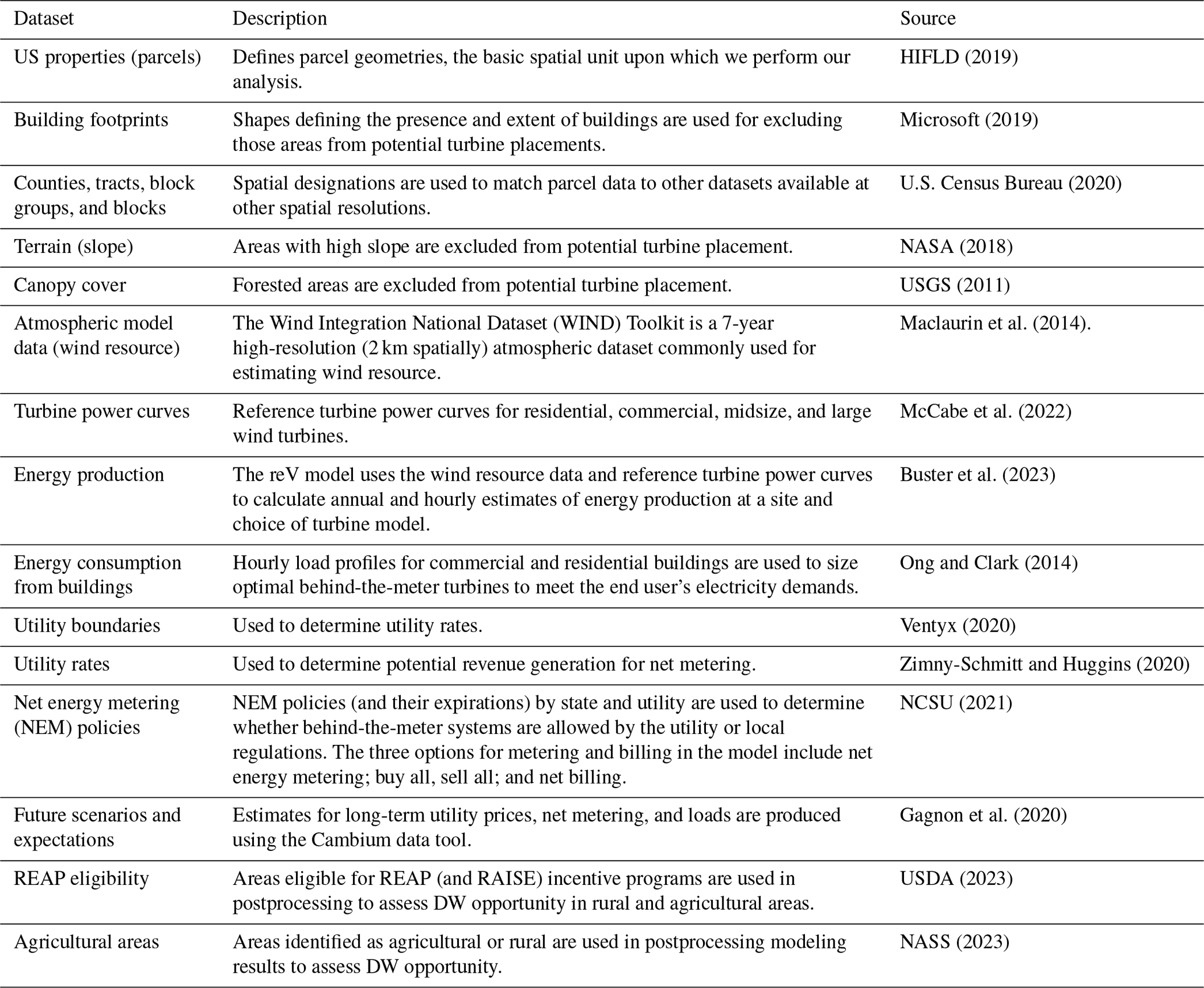
An illustration of the model workflow is included in Fig. 1. As shown in this figure, separate model components calculate different metrics throughout the model pipeline: the agent generation process sites and sizes systems to determine parcel-level technical potential, the reV model calculates annual energy production according to wind resource, and the dWind model assesses parcel-level economic potential according to local energy demand and system costs. Table 1 provides a detailed summary of the data utilized at each step of the modeling process described in Fig. 1. All data sources and vintages have remained consistent with the prior study except for U.S. Census boundary definitions (as new data from 2010 to 2020 have become available) and utility boundaries (as updated 2020 definitions have become available).

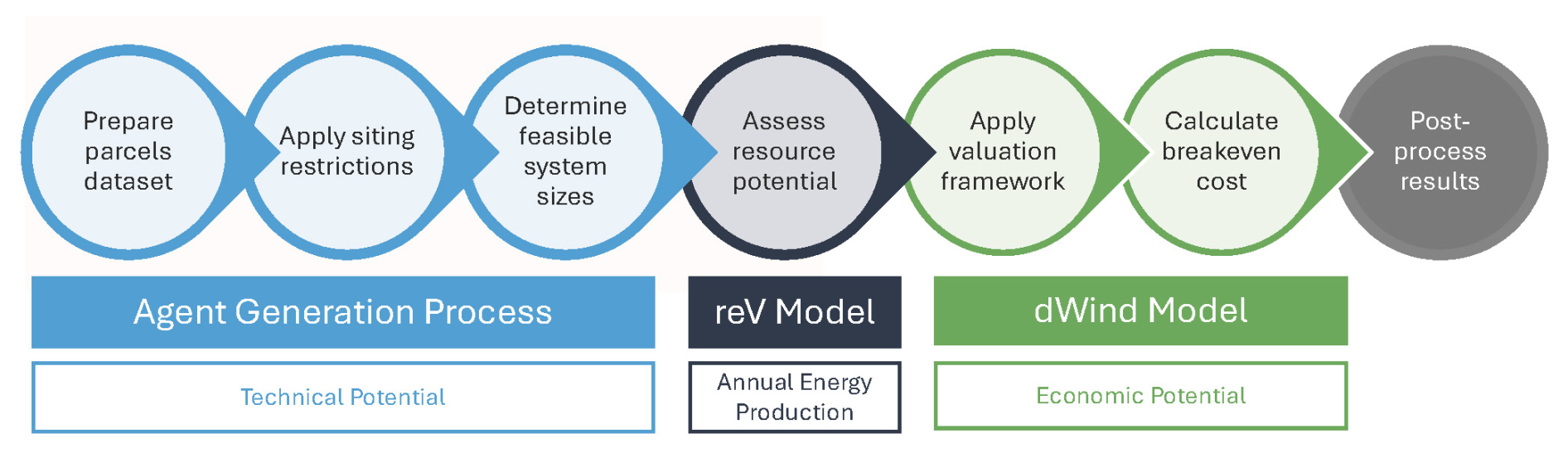
Figure 1 The modeling workflow illustrating the “decoupling” of the model components and their resulting metrics.

Table 1 Datasets used in this study.

2.2 Performance improvements and parallel scaling

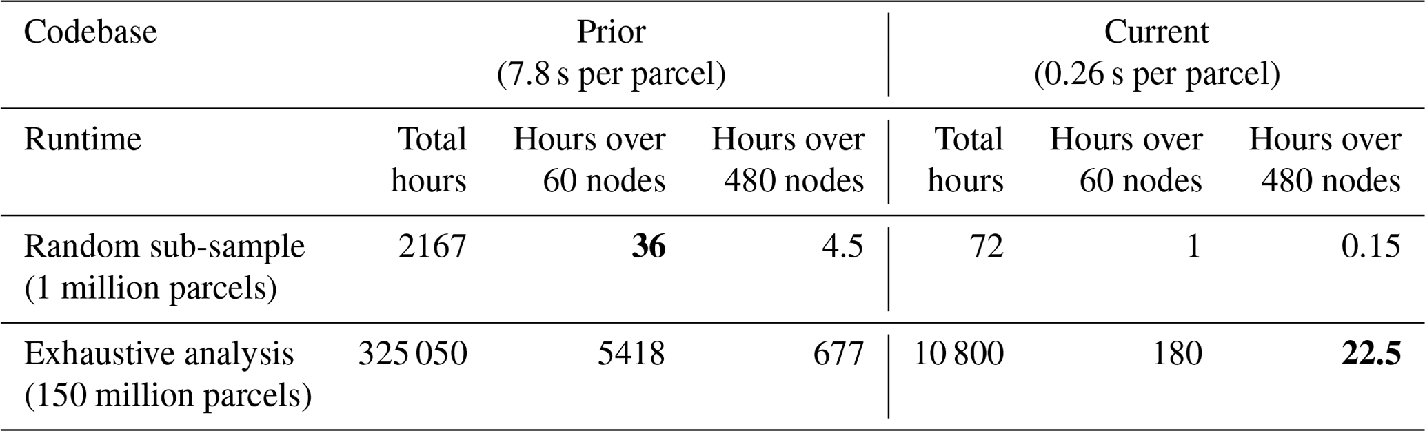
Various improvements to the dWind codebase were required to scale model runs for the full parcel dataset. The codebase from the prior version of the model had an average runtime of 7.8 s per parcel. For 1 million parcels (the number of parcels that were sampled in 2022), the total runtime of the model required 2167 h to run (or 36 h while parallelized over 60 HPC nodes). If this version of the model was scaled to run the full parcel dataset (approximately 150 million parcels), it would take a total of 325 050 h (or 5418 h parallelized over 60 nodes) to complete (which is equivalent to 226 d). Therefore, it was clear that the codebase needed to be updated to optimize performance so that the model runs could be scaled to handle a sample size approximately 150 times the size of the sample size of the previous runs from 2022.

The most significant change in the codebase to increase scalability was converting the model's former use of concurrency (or multithreading) into parallelism (or multiprocessing). Previously, at runtime, the model split the parcel-level agents into a predetermined (and configurable) number of segments and ran the bulk of the code for each chunk through a process called concurrency. Concurrency utilizes the threads within a central processing unit (CPU) to manage many processes at once (such as handling input/output operations) but is not equipped to execute many processes at once. Therefore, parallelism, or multiprocessing, is more applicable to run the dWind model at scale. In multiprocessing, processors within a system run in parallel to execute many computational tasks simultaneously, using one or more of the processor's threads (managed by the operating system rather than by the user). Converting the codebase's previous utilization of concurrency to multiprocessing reduced the average runtime per parcel from 7.8 to 0.26 s, resulting in a 97 % performance increase.

Additionally, the codebase of the model was parallelized to run simultaneously across multiple HPC nodes. In the prior model version, each model run was parallelized across a maximum of 60 nodes for a runtime of roughly 36 h per scenario. Running the new version of the model (with the full parcel dataset and code upgrades) across 60 nodes would take approximately 180 h (or 7.5 d) per scenario; when taking into consideration the full suite of scenarios that were required to run, waiting over a week per run is undesirable, despite the performance optimizations in the codebase. Therefore, the full parcel dataset was split into eight groups, and the model was parallelized across 60 nodes for each group (resulting in a total of 480 nodes per scenario). Using this grouping of the data, the full model runs to completion in less than 1 d (22.5 h) per scenario. This accelerated runtime allowed for quick postprocessing and analysis of results as well as model troubleshooting. Table 2 provides a summary of the runtime of the current model compared to the prior model, demonstrating a 30× improvement in runtime.

Table 2 Comparison of model runtime of the prior dWind codebase with the updated and optimized codebase. Text in bold represents the real time it took to run the models given the actual resources used.

2.3 Generating parcel-level representative agents

To gather the necessary parcel-level information for the dWind model, parcels are extracted from the LightBox dataset (HIFLD, 2019) and, as highlighted in Fig. 2, spatially joined to various sources to derive parcel-level data such as energy load profiles, resource generation information, and utility rates. Building footprints from the Microsoft Buildings dataset (2019) are spatially intersected with parcels and removed from parcel geometries to produce a polygon that can be used for siting distributed wind technologies. Additionally, census block geometries (U.S. Census Bureau, 2020) are spatially joined with parcels to obtain various levels of census information (such as block groups and tracts) for each parcel. Using the mapping of parcels to census information as well as preprocessed mappings of census information to various datasets such as the WIND Toolkit and the Utility Rate Database (URDB), parcels are merged with wind generation profiles and utility rates (Maclaurin et al., 2014; Zimny-Schmitt and Huggins, 2020).

Energy consumption is identified at the parcel level according to a mapping of building energy models to land use classifications (see Table A1 in the Appendix for the full mapping of parcel land use classifications to building models). Using this mapping, along with the mapping of parcels to census block groups, the average annual load and hourly load profiles (available at the block group level) are retrieved for each parcel (Ong and Clark, 2014). The load data are then scaled according to building area (identified from the Microsoft Building footprint dataset along with the LightBox parcel dataset) based on the reference floor area of the building models and their corresponding representative load profiles. Parcels are assigned an application designation of either “FOM” or “BTM”, or they may have a combined designation (“FOM, BTM”) when either application is viable for a parcel given its sector and land use categorization (the mapping of land use definitions to application is also highlighted in Table A1).

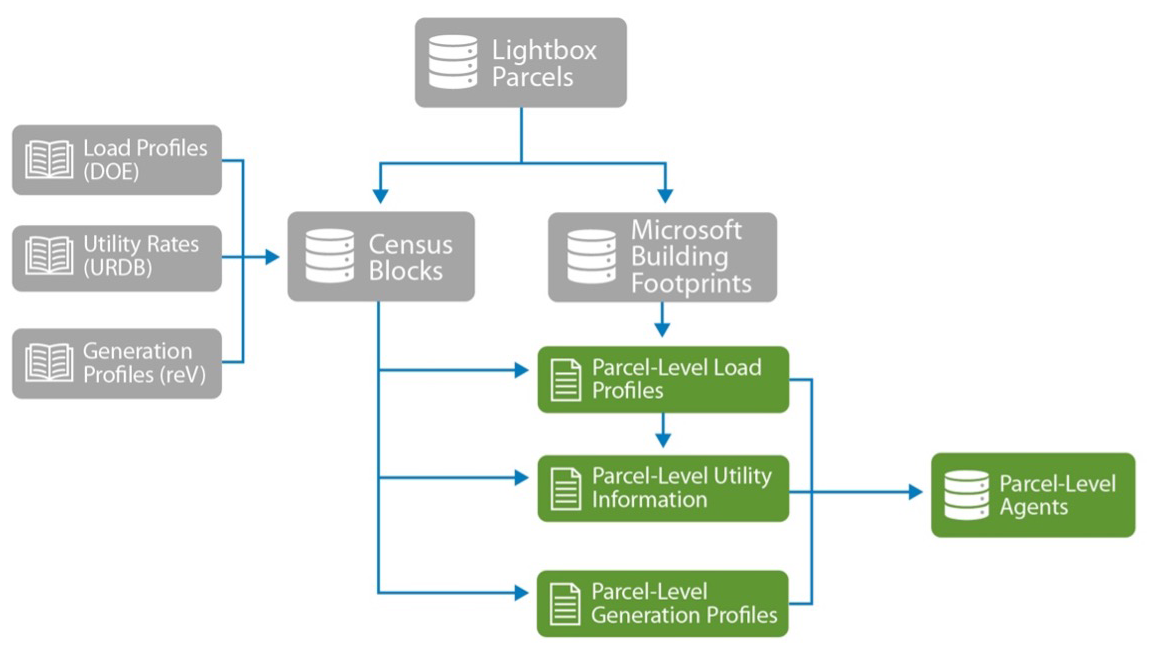
Figure 2 An illustration of the Agent Generation Data Pipeline. Parcels are joined to various data to generate parcel-level information regarding resource generation, energy consumption, and utility rates.

2.4 Modeling parcel-level technical potential

Technical potential describes the DW generation capacity that is technically feasible, with DW systems constrained solely by physical, land use, and siting exclusions. By definition, this potential corresponds to the nameplate capacity of the sited turbine and hence the maximum power output when running at rated capacity (peak power output). Only DW systems with a positive break-even cost (also understood as the “threshold CapEx” (where CapEx is capital expenditures) in McCabe et al., 2022) are considered feasible within the technical potential aggregates by region or CONUS.

To estimate parcel-level technical potential, parcel boundaries are geospatially analyzed to allow for the siting and sizing of wind turbine technologies. As outlined in Fig. 3, exclusions are removed from parcels so systems are sited on applicable areas within a parcel. The geometries that are removed from the parcel boundaries include building footprints (from the Microsoft Building footprint dataset) and steep areas that have terrain with more than 20 % slope (using a digital elevation model of CONUS) (NASA, 2018). Additionally, parcels with less than one acre (4047 m²) of land area and parcels with land use classifications that indicate physical, environmental, or cultural constraints are also excluded from siting wind technologies (see Table A2 for the full list of excluded land uses). To identify the largest possible area of land that can site a turbine, the biggest circle in the remaining parcel polygon is calculated by finding the point inside the polygon that is farthest from its edges, otherwise known as the pole of inaccessibility (Garcia-Castellanos and Lombardo, 2007).

Figure 3 Geospatial workflow of turbine siting and sizing process within parcel boundaries.

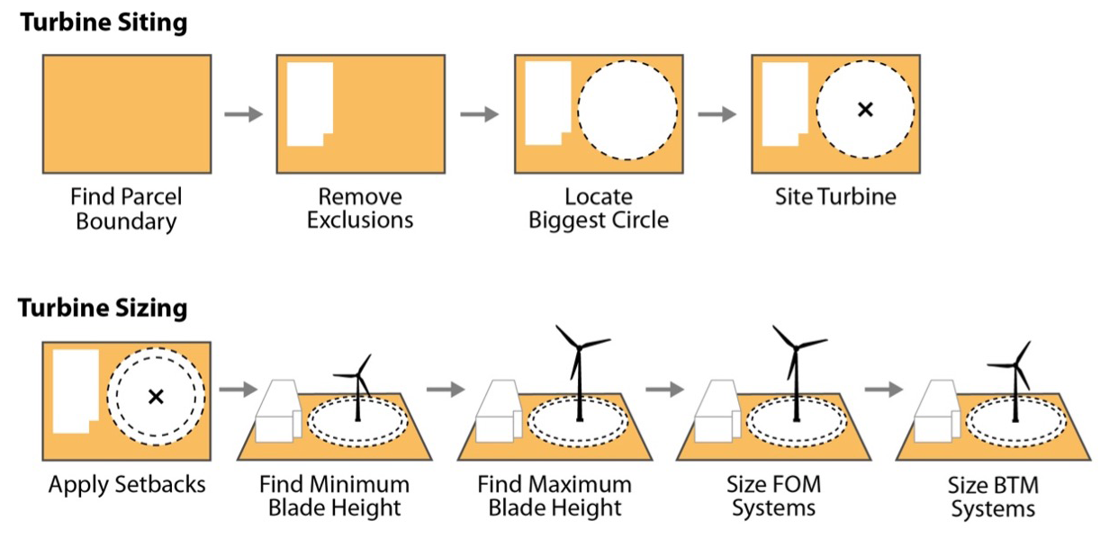
Distributed wind systems are sized according to the minimum and maximum allowable turbine blade height in each parcel. The minimum blade height is determined from canopy coverage (USGS, 2011) and canopy height information: if the canopy percent for a given census block group is greater than or equal to the required canopy clearance (set to 10 %), the minimum blade height is set to the canopy height plus 12 m (the predefined static adder for canopy height). If the canopy percent for a given census block group is less than the required canopy clearance, the minimum allowable blade height is set to zero.

$$\begin{array}{}\text{(1)}& {\text{Blade height}}_{\min }=\left\{\begin{array}{l}\text{canopy height}+\mathrm{12}\mathrm{m}\\ \text{if canopy coverage (\%)}\ge \mathrm{10}\\ \mathrm{0}\text{ if canopy coverage}<\mathrm{10}\end{array}\right.\end{array}$$

The maximum blade height is calculated according to the available land area of a parcel; if the parcel area is greater than the maximum parcel size (defined as 1 000 000 acres), the maximum blade height is set to 100 000 m, and if the area of the parcel is less than or equal to the maximum parcel size, the maximum blade height is set to the radius of the biggest circle in the parcel divided by the blade height setback factor, predefined as 1.1 times the turbine height (Lopez et al., 2021; McCabe et al., 2022).

$$\begin{array}{}\text{(2)}& {\text{Blade height}}_{\max }=\left\{\begin{array}{l}\mathrm{100}\mathrm{000}\\ \text{if parcel}>\mathrm{1}\mathrm{000}\mathrm{000}\text{acres}\\ \frac{\mathrm{radius}}{\mathrm{1.1}\times \text{turbine height}}\\ \text{if parcel}\le \mathrm{1}\mathrm{000}\mathrm{000}\text{acres}\end{array}\right.\end{array}$$

Turbine systems are classified and sized according to the minimum and maximum allowable blade height requirements calculated for each parcel using the system configuration information in Table A3. FOM system sizes are assigned as the largest turbine available for a parcel. Lastly, parcels that do not site turbines (or have a determined system size of zero) were filtered from the model pipeline.

In order to better understand and visualize the potential for DW deployments in different US environments, we selected three representative locales demonstrative of the diverse environments for potential DW opportunity in CONUS: Fort Collins, Colorado; Santa Maria, California; and Oak Ridge, Tennessee. Figure 4 provides a schematic view of available land area at the parcel level for potential deployments in these locations and represents the typical distribution of opportunity across urban, suburban, and rural landscapes. We can see from the figure that urban and suburban areas near city centers provide the greatest opportunity for smaller BTM deployments, while parcels existing outside of urban centers show opportunity for both BTM and FOM deployments.

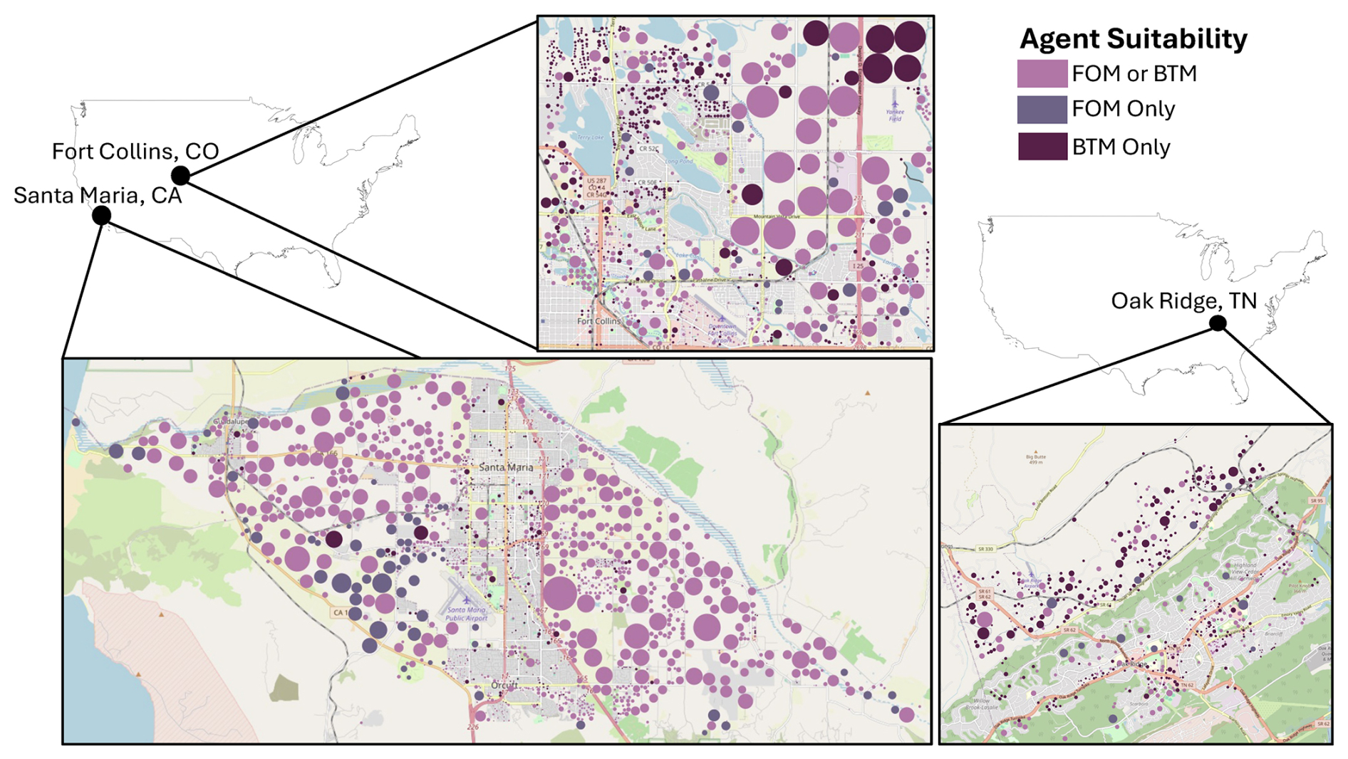
Figure 4 Visualization of DW opportunity in case study cities.

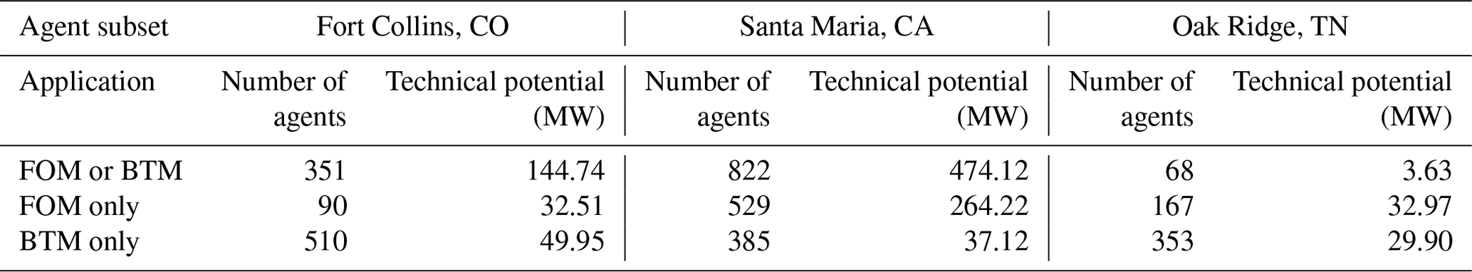
Table 3 provides a summary and comparison of the technical potential in these locales. In all three cities, the breakdown of agents by sector is roughly 56 % residential and 44 % commercial/industrial. These case studies highlight both the scale of opportunity and the diversity of potential deployment scenarios that may exist in practice.

Table 3 Summary of technical potential for case study cities.

2.5 Modeling annual energy production and economic potential

Annual energy production (AEP) is an indicator of potential energy generation for a system in an average year of operation. For DW systems, AEP is primarily based on a turbine's nameplate capacity, its capacity factor (influenced by system performance and local wind resource), and turbine availability (or how much downtime the system experiences). Using the system sizes identified for each parcel, turbines are classified as one of the following: small residential (2.5 to 20 kW), small commercial (20 to 100 kW), midsize (100 to 1000 kW), or large (1000 to 1500 kW). Using these turbine classifications and their corresponding wind performance metrics (McCabe et al., 2022), generation profiles were produced in a 2 km by 2 km grid across CONUS through the reV model. Parcel-level annual energy production and hourly resource generation profiles were derived using a spatial lookup of census block-level wind resource information to parcels.

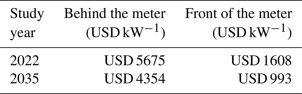
This study evaluates parcel-level locations where distributed wind can be economically deployed and aggregates them by counties and states, identifying where distributed wind is best positioned to deliver low-cost electricity to consumers and communities. Economic potential reflects potential projects and their installed capacity that would provide a positive rate of return or, in other words, be profitable for the life of the facility. The economics for distributed wind are determined in dWind using discounted cash flow analysis to determine the profitability (e.g., the payback period, net present value, and monthly electricity bill savings) over the system's lifetime. Table 4 provides the benchmark capital expenditure (USD kW⁻¹) values used as thresholds to determine economic viability in this study derived from the 2021 Cost of Wind Energy Review (Stehly and Duffy, 2022). This approach assumes that the DER value is created by reducing the electricity or fuel bills that the agent would have paid. Specifically, expenses include initial capital costs, such as the down payment and monthly loan/lease payments and annual operation and maintenance requirements. Revenue includes energy bill savings, applicable financial incentives, and tax-based credits, such as depreciation and interest rate deductions.

Table 4 Benchmark capital expenditure values used to evaluate economic potential.

2.6 Modeling different scenarios

To align with prior results and allow comparability, we produce results for a Baseline 2022 scenario (i.e., “current”) and a Baseline 2035 scenario (i.e., “future”). Both scenarios utilize baseline cost and policy assumptions for their respective year (baseline projections used for Baseline 2035) and do not deviate from the assumptions detailed in McCabe et al. (2022). Keeping scenario assumptions equal allows for a comparison between the 2022 model results (referred to here as the prior model) and the updated 2024 model results (new model), while still offering practical insight into current and future opportunity. To create parcel-level representative agents for the complete LightBox parcel dataset, agents were generated on a per-county basis using the data pipeline illustrated in Fig. 2 and then combined for national-level model runs. Since the agent generation process gathers all necessary data to run the model at the parcel level, the agent pipeline was decoupled from the dWind model so that dWind can seamlessly run valuation frameworks under different applications and scenarios by eliminating the need to generate new agents during model runtime.

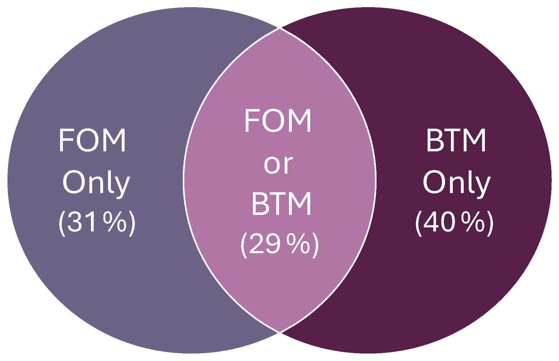
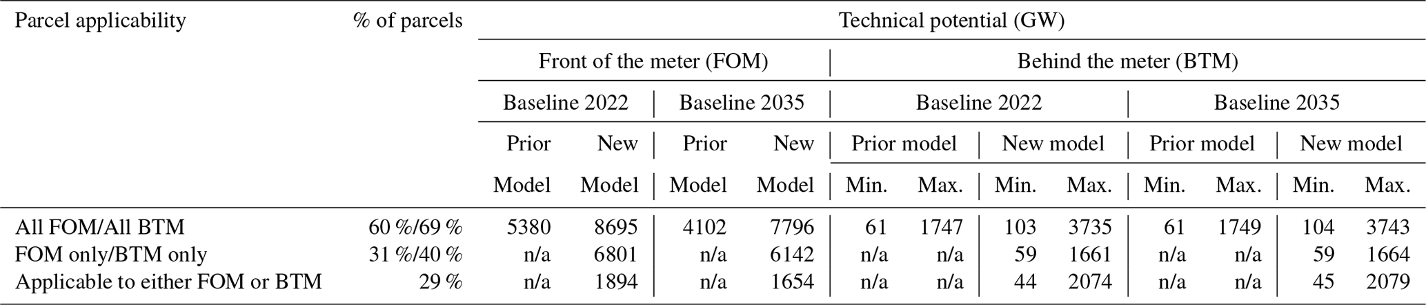
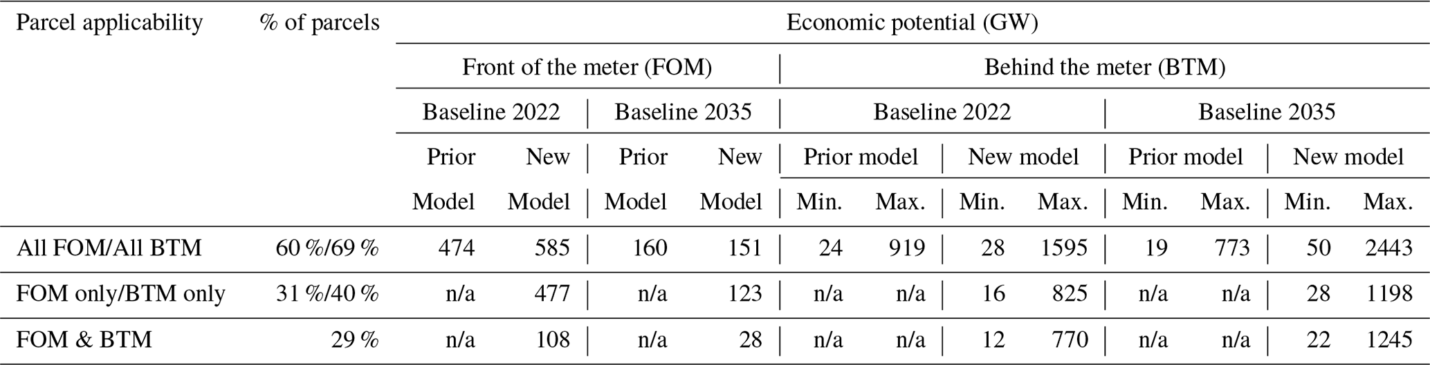
We made several key changes to how the results are represented in this study as compared to its predecessor studies. First, we expanded our analysis to increase the granularity with which we present results for each application. While the prior study presented results for BTM and FOM together, without differentiating which parcels were designated as both applications (i.e., suitable for both FOM and BTM but would ultimately only have one sited), we also consider the subset of parcels where either one or two applications are suitable (see Fig. 5). In doing so, we provide clarity on the extent of capacity that may be double-counted when looking at the two applications separately. Therefore, 60 % of parcels were identified as being applicable for FOM model runs (31 % FOM only plus 29 % FOM/BTM), and 69 % of parcels were identified as being applicable for BTM model runs (40 % BTM only and 29 % FOM/BTM).

Figure 5 An overview of the overlapping designations of parcels.

Second, we introduce the concept of “turbine downscaling” for BTM. The prior study considered the largest potential turbine in all scenarios, while we present results for this “largest” turbine scenario (termed “maximum potential”) alongside results where the turbine size is the largest turbine that would be needed to cover the energy demand of buildings on the same parcel (termed “minimum potential”). This minimum scenario describes a conservative situation wherein agents strictly avoid producing more energy than is locally needed. These two changes when taken together provide a more detailed and, we believe, realistic view of the landscape for DW opportunity.

2.7 Data aggregation and publication

In service of publishing the produced datasets so that others may use them, we make several spatial aggregations of the parcel-level data. We compute aggregate metrics at the county, ZIP code tabulation area (ZCTA), and US census block group as well as along a 2 km gridded raster. These spatial aggregates are necessary to publish the data due to underlying data licensing restrictions for the input datasets. Additionally, the aggregated data can support visualization and are often easier to use by researchers and industry scientists when performing their own analyses. Due to the size of the data, this process is also performed on NREL's high-performance computer. The process involves the calculation of zonal statistics for parcels that lie within each geography. We focus on key metrics (energy, power, break-even cost) and calculate mean, median, interquartile range, minimum, and maximum for each. Separate statistics are calculated for parcels with net present value (NPV) greater than zero and for cost-viable parcels where the break-even cost exceeds the benchmark capital expenditure. The resulting data are made available on the DOE Wind Data Portal (Phillips and Lockshin, 2024) both in GIS data format (GeoPackage) and as text-encoded data without geometries (CSV).

To enable interactive exploration of the model outputs, we created a web-based visualization platform called the Distributed Wind Scenario Analyzer, or DWSA. The platform was built using the JavaScript library React and NREL's HERO framework (https://hero.nrel.gov/, last access: 27 June 2025) and uses Uber's deck.gl to visualize the data as interactive layers on a map. The DWSA can be accessed via https://dw.nrel.gov/ (last access: 27 June 2025). Using the DWSA, a user can select a scenario by clicking the radio buttons in the control panel on the left-hand side of the map window (Fig. 6). Available selections are meter type (e.g., FOM, BTM), year, and variable to visualize (e.g., break-even cost, technical potential). Any changes to scenario selection will immediately be reflected on the map, where region fill colors correspond to variable values on a linear color scale. Additionally, the spatial resolution of the data dynamically scales based on the current zoom level. At a countrywide zoom level (as in Fig. 6), county-level resolution is displayed. As a user zooms in, the resolution will dynamically change to ZCTAs, and at maximum zoom levels, it will change to the parcel level. At all zoom levels, a user can hover their cursor over a region, and the value of the selected variable will be shown. If the user clicks on that region, a location information box will appear that contains detailed information about the selected county, ZCTA, or parcel, including links to additional information.

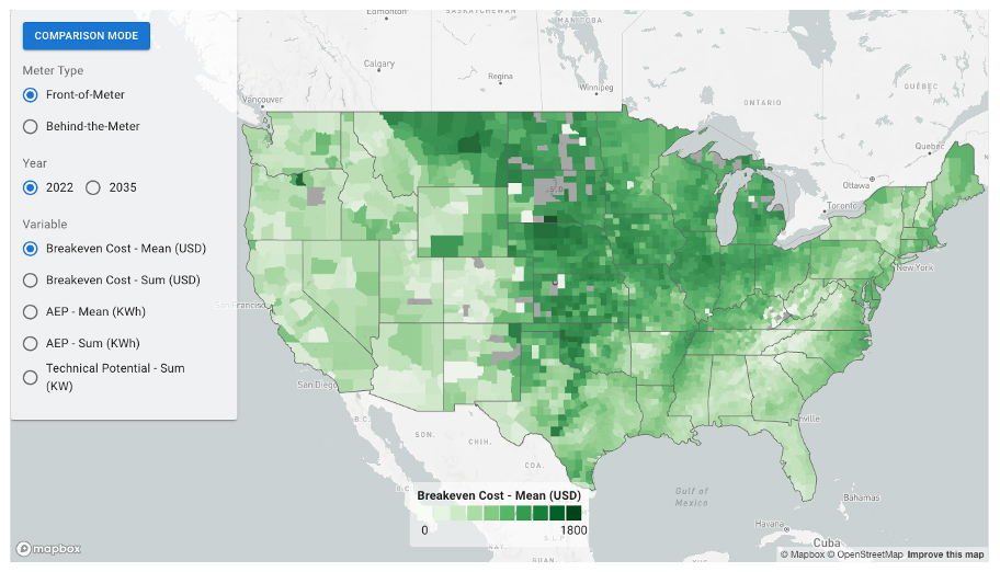
Figure 6 The Distributed Wind Scenario Analyzer facilitates exploration of model outputs and comparison of scenarios at multiple scales of resolution.

In addition to the default view “scenario mode”, the DWSA also provides a “comparison mode”, which can be toggled by clicking the button in the top left of the control panel. Comparison mode splits the map into two halves, where each half displays data from a specific scenario. The user can then update selections in the control panel to view different content side by side and drag a center divider to reveal more of less of a given scenario. By dragging across a region, visualizing differences between scenarios becomes intuitive and streamlined.

3 Results

In this section we provide the results for both FOM and BTM applications for the Baseline 2022 and Baseline 2035 scenarios, summarized and compared against prior results using the following metrics: technical potential (GW), AEP (TWh), and economic potential (GW). Additionally, opportunities for rural and agricultural parcels according to the new results are identified. Please note that while 29 % of parcels are suitable for both FOM and BTM applications, the maps presented for each scenario include these parcels with their respective metrics for the identified scenario (i.e., either FOM or BTM metrics).

3.1 Technical and economic potential

Table 5 provides a summary of national opportunity for DW, highlighting more than 8600 GW of current FOM potential and 3735 GW of BTM potential (103 GW with downsized turbines). Future (2035) scenarios show a slight decrease in opportunity owing to the sunsetting of key policy incentives. Technical potential of both the Baseline 2022 and Baseline 2035 scenarios in the new results increased from the prior model results. Specifically, the technical potential of the Baseline 2022 scenario increased by 3315 GW, and the Baseline 2035 scenario increased by 3694 GW, indicating an average of 1.8× the amount of technical potential previously reported. For BTM applications, our results show an average increase in technical potential of 2.1× from the prior model runs (for maximum potential): the Baseline 2022 technical potential increased by 1988 GW, and the Baseline 2035 technical potential increased by 1994 GW. We believe this new result constitutes a more accurate and complete depiction of DW opportunity in CONUS and shows the substantial opportunity that exists nationally.

Table 5 Technical potential results comparison for current and future scenarios.

n/a: not applicable

Looking next to those parcels for which the available generation is also economically suitable, Table 6 provides a comparable summary. We see that with the described model improvements, the economic potential for FOM applications increased by 111 GW for the Baseline 2022 scenario but slightly decreased (by 9 GW) in the Baseline 2035 scenario. For BTM applications, however, economic potential of both the Baseline 2022 and Baseline 2035 scenarios in the new results increased significantly from prior model results (for maximum potential): the Baseline 2022 economic potential increased by 676 GW, and the Baseline 2035 economic potential increased by 1670 GW; this indicates an average increase in economic potential of 2.5× from what has been previously reported.

Table 6 Economic potential results from 2022 and 2024 models.

n/a: not applicable

Figure 7 provides a graphical representation of the economic potential in CONUS. These figures show opportunity for both FOM and BTM in the Baseline 2022 (current) and Baseline 2035 (future) scenarios. The figures highlight the relatively large opportunity in the central “wind belt” along the US Midwest, including counties in Texas, Oklahoma, Nebraska, Montana, and Wyoming, in addition to parts of California and New England (e.g., Maine). Overall, there are substantially more counties that may benefit from BTM DW deployment when viewed in the context of economic constraints. Nonetheless, the economic potential of BTM parcels is highly dependent on whether the largest possible turbine is sited (which is generally the most economically favorable) or if the turbine is downsized to load (which is generally less favorable than FOM).

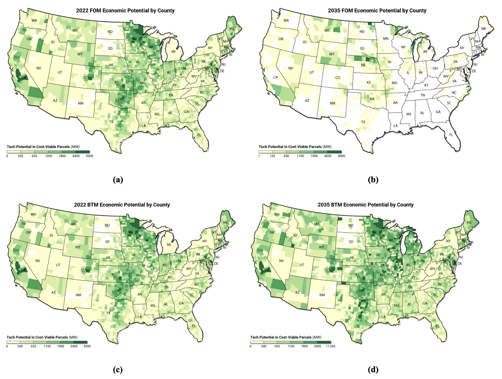
Figure 7 Economic potential for DW in CONUS as measured in megawatts for every county and every suitable land parcel within those counties. The subfigures provide results for four scenarios: (a) FOM 2022, (b) FOM 2035, (c) BTM 2022, and (d) BTM 2035. The results show significant opportunity for FOM in the middle region of the country with higher wind speeds as well as some opportunities in coastal regions and New England. The BTM results show substantial opportunity throughout the country but with relatively more opportunity in the central wind belt, Midwest, California, and Maine. In these figures, the maximum BTM turbine has been used to show maximum capacity, rather than the downsized turbine.

Economic potential can also be understood through supply curves that describe the cumulative capacity by levelized cost of energy (LCOE), as presented in Fig. 8. The inflection point, or elbow, in these plots indicates the sensitivity of cost to increased capacity beyond the point of critical economic value. The supply curve for FOM shows LCOE values in line with land-based utility-scale wind energy LCOE (as compared to the NREL Annual Technology Baseline), with about 7000 GW having an LCOE lower than USD 30 MWh⁻¹ across both Baseline 2022 and Baseline 2035. For BTM (using the minimum potential), the supply curves show a large range in LCOE values: a cumulative capacity of approximately 100 GW has an LCOE of USD 400 MWh⁻¹ for Baseline 2022 and Baseline 2035, with lower LCOE overall for the future scenario.

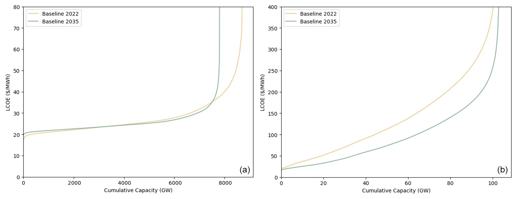
Figure 8 Cumulative capacity by levelized cost of energy (LCOE) for FOM (a) and minimum BTM (b). These plots demonstrate the relationship between cost and capacity with the inflection point or elbow, beyond which cost to expand capacity exceeds practical values.

3.2 Annual energy production

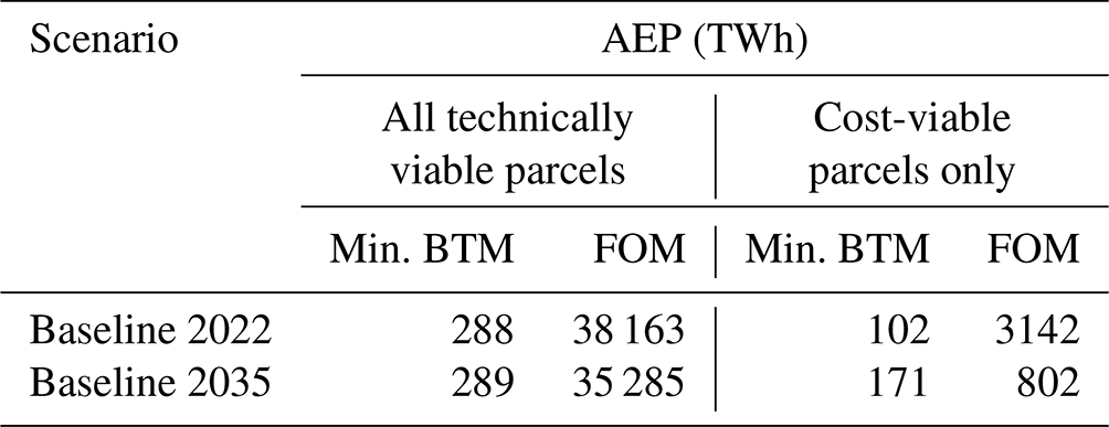
The AEP for DW was calculated for all technically viable parcels (parcels with technical potential for DW) and for cost-viable parcels (parcels with economic potential for DW) only (Table 7). Technically viable AEP is much larger than cost-viable AEP across scenarios (about 3× for minimum BTM and over 10× for FOM). When comparing between applications, FOM AEP is approximately 2.2× larger than minimum BTM AEP. This metric highlights the enormous potential for energy generation potential for FOM deployments (more than 38 000 TWh), meaningfully limited by current economic constraints (3100 TWh). Insofar as policies may provide incentives for FOM deployments and unlock additional potential, this is an important result. Downscaled (minimum) BTM opportunity is much more modest in scale but still offers a substantial energy generation potential at 288 TWh for all parcels and 102 TWh for the subset of cost-viable (profitable) parcels. Compared to the estimated 4000 TWh of electricity consumption in the United States (DOE, 2024), this figure suggests that a substantial fraction of that energy could be generated with DW. Taking the most conservative estimates, 2.5 % of demand could be satisfied using economic BTM scenarios and an additional 78.5 % of demand could be satisfied with economic FOM scenarios. Additional incentives for deployment or more favorable net metering regulations (for BTM scenarios) would allow an even greater potential.

Table 7 Annual energy production for technically viable and cost-viable parcels in CONUS.

Finally, Fig. 9 shows the distribution of AEP (aggregated by county) across CONUS for all technically viable parcels for DW (regardless of economic viability) to allow inspection of geospatial distribution of these opportunities. While significant opportunity exists in all states, we observe higher AEP for both FOM and BTM applications across the majority of the Midwest and in some parts of California and the Northeast. These trends are consistent across the technical and economic potential metrics.

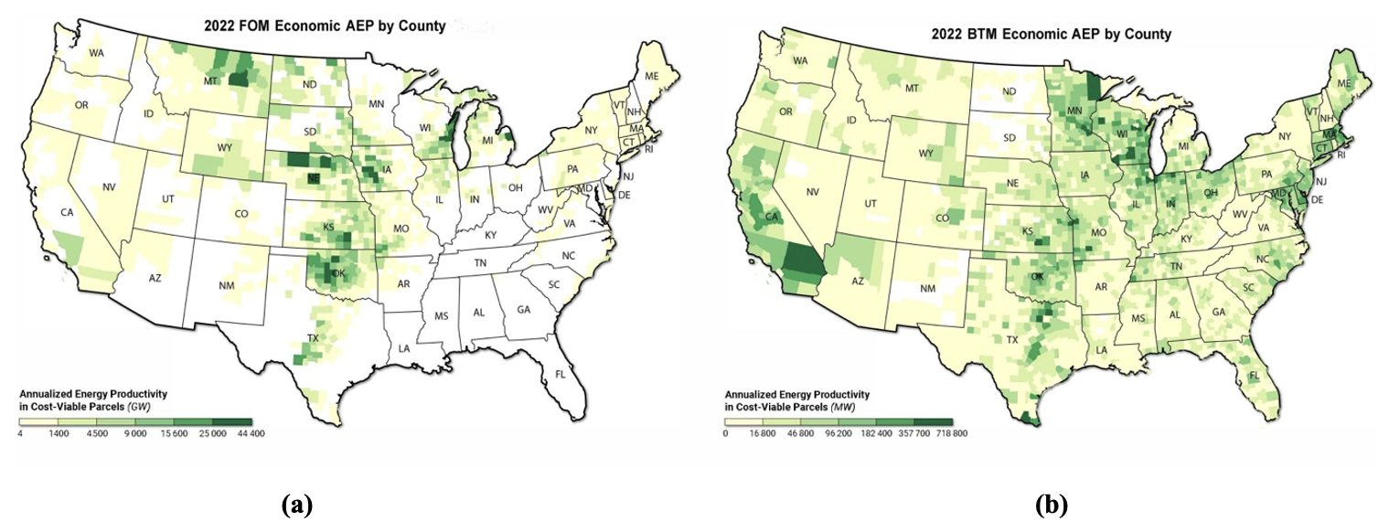
Figure 9 Annual energy production for technically viable DW in CONUS as measured in kilowatt hours for every county and every suitable land parcel within those counties for (a) Baseline 2022 FOM and (b) Baseline 2022 BTM.

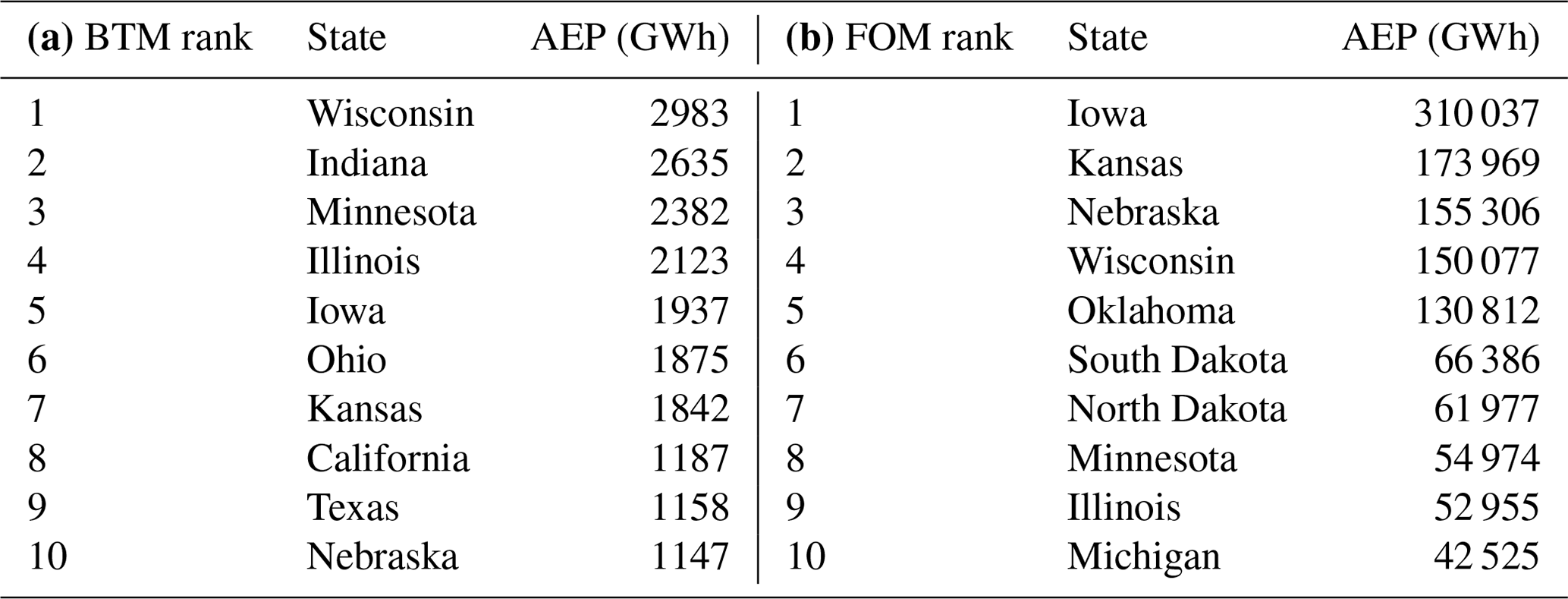
Table 8 Top 10 CONUS states based on agricultural cost-viable AEP (GWh) by CroplandCROS land use (excluding REAP-ineligible areas) according to (a) BTM 2022 and (b) FOM 2022 model results.

3.3 Opportunities for rural and agricultural parcels

Due to recent investments in incentives for DW deployment in rural and agricultural areas through the RAISE initiative, we also seek to highlight potential unique opportunities in this sector. To calculate AEP for cost-viable rural and agricultural parcels, REAP-eligible model results at the census-block-group level were overlaid with the USDA 2023 national cropland data layer (NASS, 2023), which classifies CONUS into a 30 m resolution grid of land use type (areas classified as agricultural land in the CroplandCROS dataset are identified in Table A3). The benefit of using the CroplandCROS dataset is the ability to break the analysis down to specific crop types, though the results presented here use a simplification of those categories (e.g., all crops have been combined into “agricultural”). Then, the relative proportion of agricultural land in each block group is calculated to estimate the DW opportunity in these areas.

One critical assumption used by this approach is that the DW results are evenly spread across the block group. The model produces turbine locations that could be modeled as single points, which would only have one land use type each. However, real-world turbine placement is governed by many site-specific factors that cannot practically be modeled. Using the turbine positions proposed by the model to determine land use may give false precision, whereas the more probabilistic approach described above may give a closer estimate of real-world land use. Additionally, using smaller DW polygons (i.e., parcel-level results) could give more accurate results at the cost of greater computational requirements.

Table 8 highlights the top 10 states in CONUS for cost-viable generation in agricultural/rural areas for the 2022 BTM and FOM scenarios. Much of the agricultural DW opportunity for both the BTM and FOM scenarios is in the Midwest due to the region's availability of agricultural land as well as the area's wind resource.

These results suggest there is a substantial opportunity for DW on agricultural land. Overall, agricultural land represents 33 % of the total DW opportunity for the 2022 BTM scenario and 42 % for FOM 2022, indicating that agricultural and rural areas represent the greatest opportunity for DW, more than any other land use type.

4 Discussion and conclusion

The work presented here represents a significant advancement in depth, resolution, and rigor in understanding the technical and economic potential of DW energy across the contiguous United States. This study demonstrates the increased efficiency and capability of the dWind model, which now operates 30 times faster than prior versions and can handle an entire dataset of over 150 million parcels, compared to the sample of 1 million parcels used previously. These improvements are largely attributed to the shift from concurrency to parallel processing, which drastically reduced runtime per parcel, enabling more granular, parcel-level analysis across the country. Meanwhile, improvements to parcel selection, siting, and turbine downsizing have improved the accuracy and realism of model estimates.

The findings show that the potential for DW energy is considerably higher than previously estimated. We calculate that there is 8695 GW of DW technical potential for FOM applications in the Baseline 2022 scenario and 7796 GW in the Baseline 2035 scenario, which is, on average, 1.8 times more technical potential in CONUS than previously reported. Similarly, there is, on average, 2.1 times more technical potential for BTM applications: 1749 GW in the Baseline 2022 scenario and 3743 GW in the Baseline 2035 scenario. The improved model also highlights additional economic potential for BTM applications, demonstrating DW's promise as a cost-effective renewable energy source. Compared to the estimated 4000 TWh of electricity consumption in the United States (DOE, 2024), a substantial fraction of that energy could be generated with DW. Taking the most conservative estimates, 2.5 % of demand could be satisfied using economic BTM scenarios and an additional 78.5 % of demand could be satisfied with economic FOM scenarios. Additional incentives for deployment or more favorable net metering regulations (for BTM scenarios) would allow an even greater potential. In alignment with recent USDA/DOE incentive programs, we also note significant existing opportunity for DW generation in agricultural and rural areas: the top 10 states for FOM systems have an AEP of 1199 TWh, and the top 10 states for BTM applications have an AEP of 19 TWh.

However, like any modeling approach that provides estimates about the future, this analysis has limitations. Firstly, the analysis was only performed on the contiguous United States. Likewise, there is an opportunity in the future for the in-depth exploration of uncertainties in the results. Key sources of uncertainties most critically derive from inherent uncertainties in the data sources, including electrical demand derived from building loads, parcel data completeness and land use, canopy cover, and exclusions including slope of terrain. Beyond this, there is specific uncertainty in adoption rate, and presently agents make independent decisions, while in practice adoption may follow a more organic growth model. In future work we hope to incorporate agentic decision-making and expressly model adoption rates to understand the potential for DW over time. Lastly, our study considers the siting of one turbine per parcel, and in future work we hope to explore multi-turbine siting, when appropriate, as well as hybrid system designs that incorporate some aspect of energy storage and photovoltaic generation.

Despite these limitations this work marks a significant degree of progress towards large-scale high-resolution modeling of DW potential. The granular data provided by the updated dWind model will be invaluable for policymakers, industry stakeholders, and property owners, enabling them to make more informed decisions regarding DW implementation. The framework described here is designed to be universal and adaptable, allowing extension to additional domains and modeling of arbitrarily complex technology scenarios and adoption processes. By offering insights on site-specific feasibility and economic return, the model supports strategic planning, incentive design, and market expansion for DW technology. In summary, the enhanced model described here serves as a comprehensive tool for accelerating the adoption of distributed wind energy, particularly in rural and agricultural areas, and marks an essential step toward a more resilient and sustainable energy infrastructure in the United States.

Appendix A

Table A1 Parcel land uses categorized by sector, technology application, and associated building model.

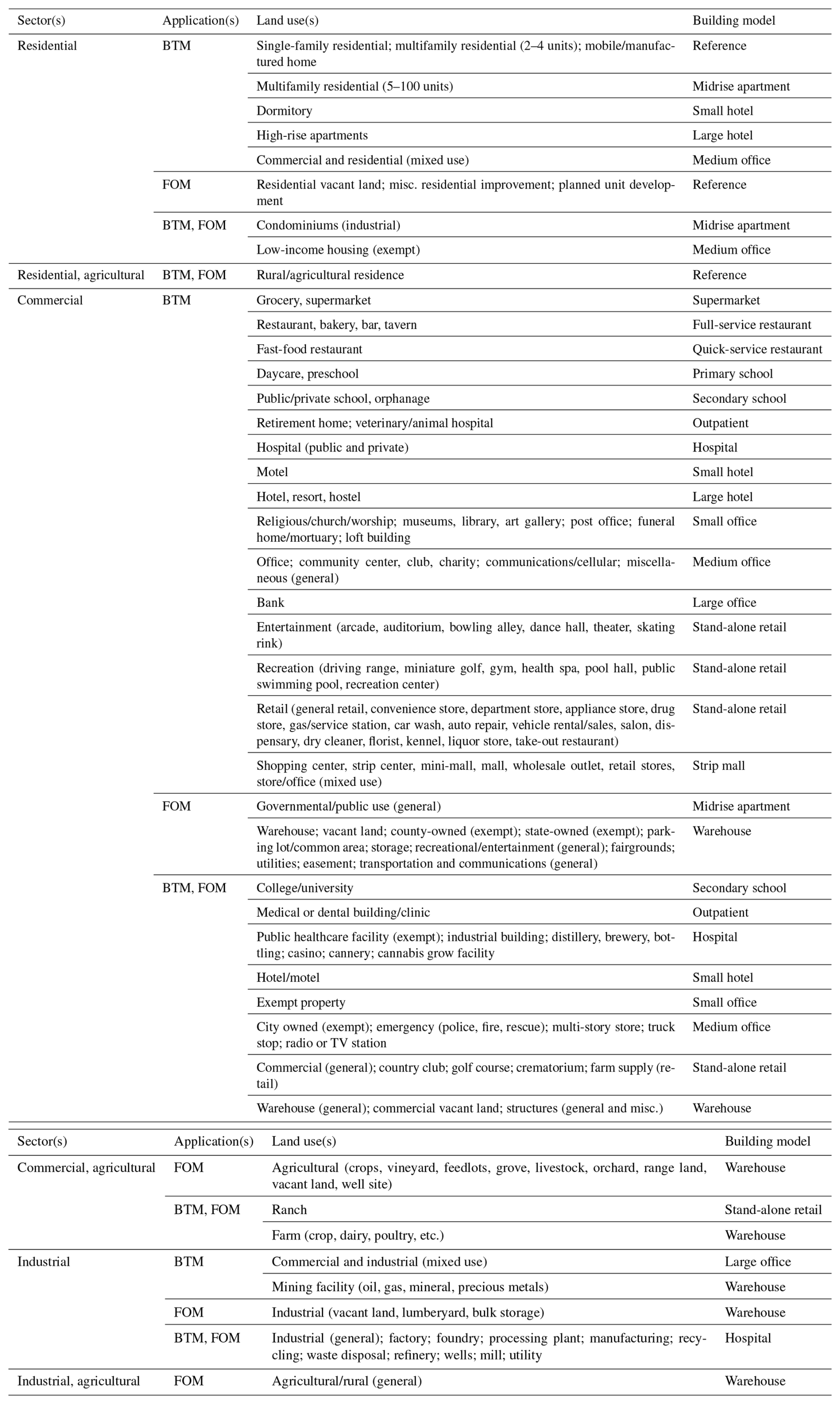
Table A2 Parcel land use types excluded for distributed energy resource development.

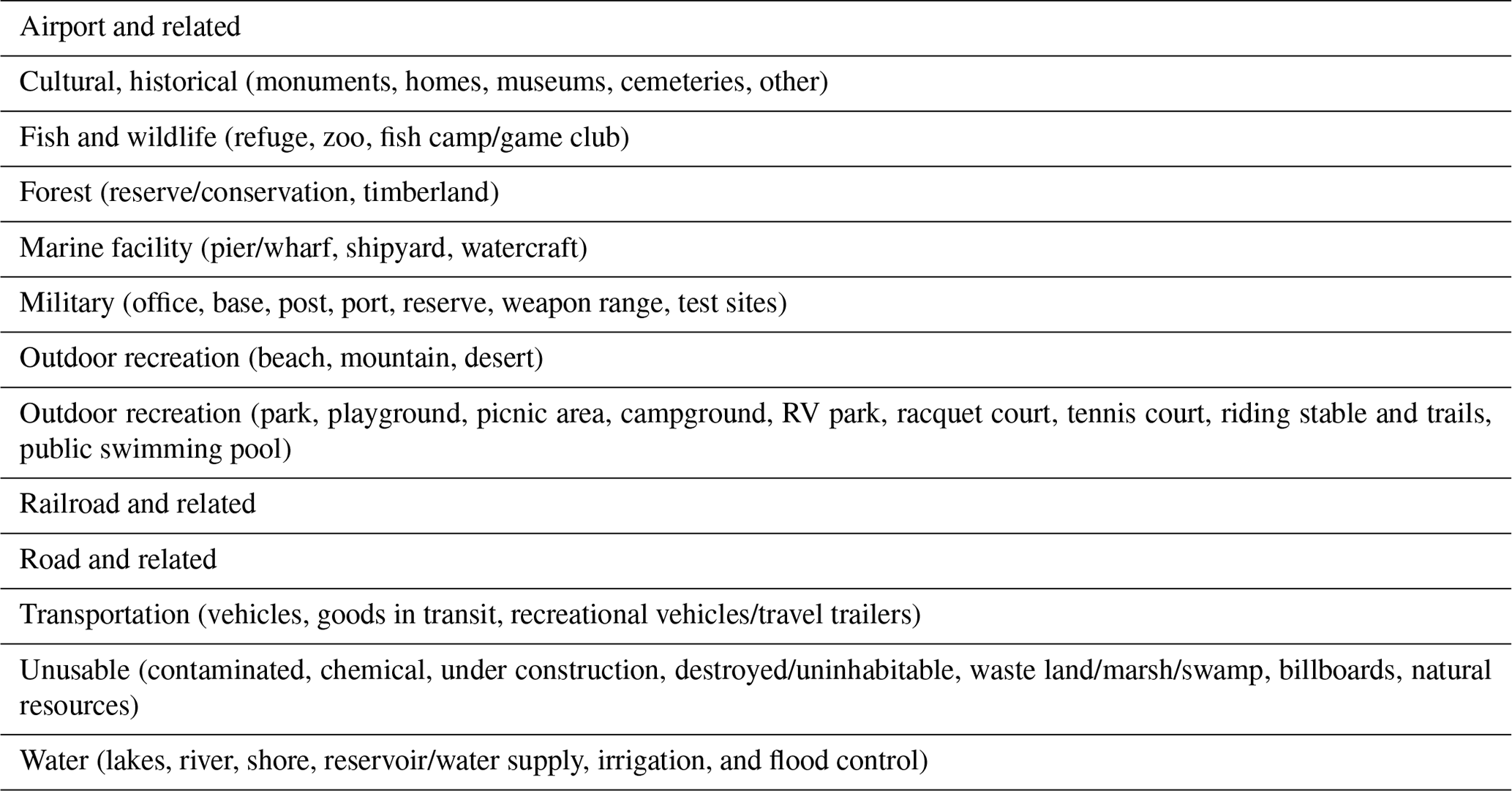
Table A3 Blade heights for various turbine sizes and height configurations.

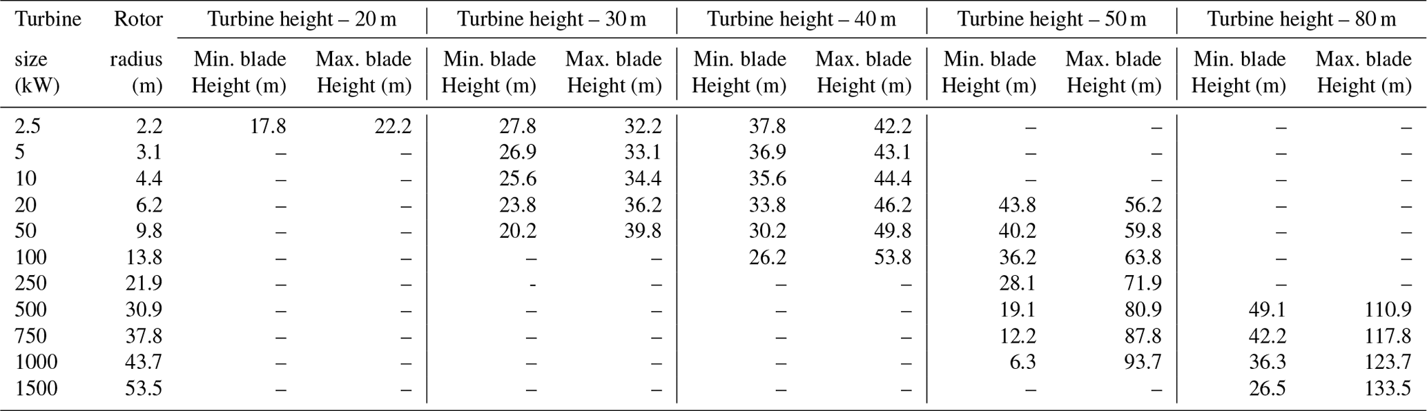
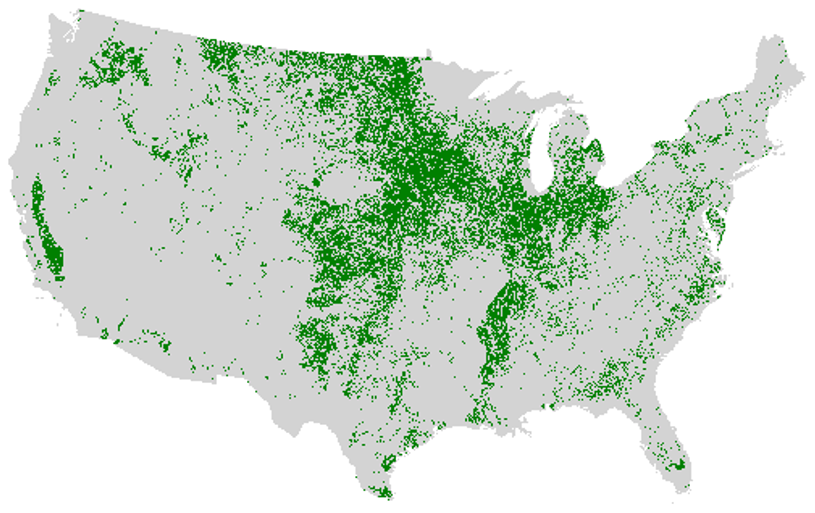
Figure A1 Areas classified as agricultural land in the CroplandCROS dataset. The prevalence of agricultural land in the midwestern states gives them the greatest opportunity for distributed wind production on agricultural land.