Output-constrained individual pitch control methods using the multiblade coordinate transformation: trading off actuation effort and blade fatigue load reduction for wind turbines

Individual pitch control (IPC) has been thoroughly researched for its ability to reduce wind turbine blade and tower fatigue loads. Conventional IPC often uses the multiblade coordinate (MBC) transformation and aims for full attenuation of the oscillating loads. However, this also leads to high control effort and increased fatigue damage on the pitch system. Output-constrained IPC uses the minimum actuator effort to drive loads to some reference value instead of fully attenuating them, achieving a trade-off between load reduction and actuator effort. To date, no control method exists that achieves output-constrained IPC using the conventional MBC approach. Furthermore, while multiple constrained IPC approaches have been proposed and analyzed, none of them analyze the full range of operating points between “no IPC” and “full IPC”. This paper presents two output-constrained IPC methods that use the MBC transformation. The first method, ℓ^∞ IPC, independently drives the tilt and yaw moment to a tilt and yaw reference, while the second method, ℓ² IPC, directly targets the magnitude of the combined tilt and yaw load. We furthermore analyze all operating points between no IPC and full IPC. OpenFAST simulations of the IEA 15 MW turbine were run at a wind speed of 15 m s⁻¹. In laminar conditions, ℓ² IPC is more efficient because it reduces the magnitude of the load directly, while ℓ^∞ IPC also uses control effort to change the phase of the blade load in the direction of the load references. To assess the performance in realistic wind conditions, results are averaged over multiple turbulent wind seeds. Both ℓ^∞ IPC and ℓ² IPC have a similar performance, and the operating points between no IPC and full IPC form a nonlinear trade-off. One of the operating points in this trade-off achieves a 50 % load reduction, measured in damage equivalent load, with just 16.4 % of the actuator effort, measured in actuator duty cycle, compared to conventional IPC with the same integrator gain. This shows the potential of output-constrained IPC to facilitate a superior trade-off between load reduction and actuator effort.

1 Introduction

Wind energy has become a mainstream energy provider due to its severe cost reduction in recent decades. This cost reduction was, in part, driven by engineering efforts that enabled taller towers, longer blades, and higher capacity factors of wind turbines (Veers et al., 2019). However, longer blades are more flexible and sample a larger area of the spatially and temporally varying wind field, making them susceptible to fatigue loading and causing new challenges.

Individual pitch control (IPC) can alleviate some of these fatigue loads by pitching the three blades independently to reduce the periodic loading that arises from effects such as wind shear, tower shadow, turbulence, and rotor misalignment (Bossanyi, 2003). This could decrease the material cost of the wind turbine and/or increase its lifespan (Pettas et al., 2018).

IPC implementations using classical control techniques often use the multiblade coordinate (MBC) transformation (Bir, 2008), also called the Park or d–q transformation, originating from electrical engineering (Park, 1929), or Coleman transformation, originating from helicopter rotor control (Coleman and Feingold, 1958). The MBC transformation converts signals from a rotating reference frame to a stationary reference frame and vice versa. In the context of three-bladed wind turbines, it transforms a set of three signals from the rotating blade frame to a set of three signals in the nonrotating frame, usually referred to as collective, tilt, and yaw components, which represent the rotor as a whole. By converting the blade dynamics to rotor dynamics in the nonrotating frame, they can be analyzed together in a common reference frame with the other nonrotating components, such as the tower (Bir, 2008).

The MBC transformation can also be used to control oscillations in blade loads. The forward transformation then converts these loads to steady tilt and yaw moments in the nonrotating frame. These tilt and yaw moments are then driven to zero by two independent SISO controllers, typically integral (I) or proportional–integral (PI) controllers, which produce a tilt and yaw pitch signal. These outputs are subsequently transformed back to the rotating frame using the inverse MBC transformation, resulting in a sinusoidal pitch signal that has a 120° offset between each blade (Bossanyi, 2003, 2005; van Solingen and van Wingerden, 2015). The dominant load contributing to blade fatigue is the 1P (once-per-revolution) oscillation, mainly due to wind shear (Kragh et al., 2012). This 1P oscillation can be reduced by a 1P IPC controller. However, the 2P harmonic can also be reduced by using a 2P MBC transformation. While the 2P harmonic typically contributes less to the fatigue damage of the blade, since its magnitude is smaller, it contributes to fatigue damage on the tower since the 2P blade load maps to a 3P oscillation on the tower (van Solingen and van Wingerden, 2015; Bossanyi et al., 2013).

Due to the rotation of the blades and system dynamics arising from, e.g., actuator and blade dynamics, the tilt and yaw axes are coupled (Mulders et al., 2019). For flexible wind turbines, these dynamics are slower and thus lead to a strong coupling between the tilt and yaw axes. This coupling necessitates a multivariable controller design (Bossanyi, 2003; Lu et al., 2015) or decoupling of the tilt and yaw axes, enabling SISO controller design. This can be achieved by using an azimuth offset in the inverse MBC transformation, as was already noted by Bossanyi (2003) and formally analyzed by Mulders et al. (2019) and Mulders and van Wingerden (2019), who also provide a method to find the optimal azimuth offset.

Several field tests demonstrating the load reduction capabilities of IPC have been carried out (Bossanyi et al., 2013; Shan et al., 2013; Van Solingen et al., 2016; Ossmann et al., 2021). However, since conventional IPC always aims for complete load alleviation, it leads to higher pitch actuation. This higher actuation leads to excessive pitch wear (Schwack et al., 2016) and requires a higher thermal rating of the pitch system (Burton et al., 2021), preventing adoption of IPC using existing designs. This has hindered industry adoption (Novaes Menezes et al., 2018). A control method that balances load reduction and pitch actuation would make IPC more practically feasible.

Three methods to constrain IPC controllers can be distinguished that enable the trade-off between load reductions and pitch activity: input-constrained IPC, where the actuator angle, rate, and/or acceleration are limited; output-constrained IPC, where the amplitude of the oscillating loads is regulated; and fatigue-constrained IPC, which aims to directly constrain the fatigue damage. To analyze these three methods, we also define a baseline operation without IPC as “no IPC” and conventional, unconstrained IPC as “full IPC”.

Input-constrained IPC can be implemented when using the MBC transformation by realizing that the resulting blade pitch signal is sinusoidal, of which the maximum, maximum rate, and maximum acceleration can be derived using the amplitude of the pitch signal in the nonrotating domain and rotor speed. Bossanyi (2005) introduces a limit schedule that limits the output of the PI controller in the nonrotating frame, thus limiting the pitch angle for each blade. Kanev and van Engelen (2009) extend this and use an anti-windup strategy to limit the pitch angle, rate, and acceleration. The previous studies assume a constant rotor speed, while Ungurán et al. (2019) also derive angle and rate limits for non-constant rotor speeds. They furthermore note that adding a rate limit causes a time lag in the pitch signal, which slightly reduces the efficiency of IPC.

Input constraints can also be implemented when using a model predictive control (MPC) method by including additional constraints in the optimization problem that is solved during each time step. Raach et al. (2014) include actuator constraints in a nonlinear MPC framework. Petrović et al. (2021) propose a method to convexify these constraints to get a convex optimal control problem when using MPC. Lastly, Liu et al. (2021) include input constraints in a constrained subspace predictive repetitive control (cSPRC) framework, a data-driven MPC controller.

Output-constrained IPC sets limits on the permissible loads and employs the minimal pitch signal required to maintain the loads within these limits, thus opting for no IPC action when the loads naturally fall within these limits. Liu et al. (2022) later used the same cSPRC framework to constrain the periodic blade loads rather than the pitch angles to form an output-constrained IPC method. Henry et al. (2024) use the MBC transformation and set a positive reference on the tilt axis, thus only constraining the positive tilt load and assuming a negligible yaw moment.

Fatigue-constrained IPC sets direct bounds on the fatigue damage that may be accumulated. Since the fatigue calculation is usually algebraic and highly nonlinear, Collet et al. (2021) derive a convex, data-driven objective function that can approximate the fatigue damage on both the blades and the actuators. Their MPC controller can find a trade-off between blade fatigue and actuator activity by weighting the fatigue damage differently for the blade and actuator fatigue damage.

Comparing these methods, we see that output-constrained IPC sets limits on permissible loads and employs the minimal pitch signal required to maintain these loads within the specified bounds. When the loads naturally fall within these reference bounds, the controller refrains from IPC action. In contrast, input-constrained IPC consistently actuates the pitch but never exceeds a maximum pitching angle, rate, or acceleration. Fatigue-constrained IPC poses challenges due to the nature of fatigue damage calculation. The conventional approach of rainflow counting to get a damage equivalent load cannot be done in real time, thus requiring estimation techniques.

Consequently, output-constrained IPC emerges as a promising method to balance load reduction and pitch actuation when constraints on loads are more important than constraints on actuation. Furthermore, the load references could be integrated into the wind turbine design process, thus enabling control co-design of the wind turbine (Pao et al., 2024) with IPC, realizing its potential for material reduction. However, little research has focused on this approach, and some output-constrained IPC methods rely on data-driven techniques that are not commonly used in industry or only constrain a positive tilt moment. Additionally, while any constrained IPC method can explore the operation space between no IPC and full IPC, the complete trade-off, to the best of our knowledge, has not been investigated. Notably, though, both Han and Leithead (2015) and Lara et al. (2024) have explored a small portion of this space by adjusting the gains of IPC controllers, thus showing the trade-off when operating close to full IPC.

This work explores the full operating region between no and full IPC using two different output-constrained IPC controllers using classical control elements and the MBC transformation. The first method, ℓ^∞ IPC, constrains the tilt and yaw moments independently, while the second method, ℓ² IPC, constrains the magnitude of the combined tilt and yaw moment. So this work provides the following contributions:

1. proposing two output-constrained control methods: ℓ^∞ IPC and ℓ² IPC;

2. deriving the open-loop load estimator, used by both control methods;

3. sharing the two output-constrained control methods in an open and freely accessible online repository (Hummel, 2024);

4. analyzing the working mechanism of these controllers in laminar conditions;

5. analyzing the trade-off between fatigue load and pitch actuation when operating at any operating point between no and full IPC in both laminar and turbulent flow conditions.

In this work, we refer to the IPC methods that aim for full load alleviation as conventional, unconstrained, or full IPC. When only the collective pitch controller is active, this is referred to as no IPC. Furthermore, this work focuses on blade loads only and thus only on 1P IPC. However, by adding additional MBC loops, the proposed control methods could be easily extended to higher harmonics.

This paper proceeds as follows. First, the MBC transformation and its use for IPC is discussed in Sect. 2. An illustrative example of using controller tuning with conventional IPC to achieve a trade-off between load reduction and actuator effort is given in Sect. 3. Next, the two output-constrained IPC controllers are introduced in Sect. 4. The results of the controllers are presented in Sect. 5. Finally, conclusions are drawn in Sect. 6.

2 Individual pitch control using the multiblade coordinate transformation

This section provides an overview of individual pitch control using the MBC transformation. Besides general theory, the rotations that lie at the fundament of the MBC transformations are shown, and how these rotations are used to decouple the orthogonal tilt and yaw axes using an azimuth offset is discussed.

2.1 Motivation behind the MBC transformation

The MBC transformation transforms a set of three signals from a rotating reference frame to a nonrotating reference frame or vice versa. It has proven helpful in two ways in the wind turbine field: system analysis and control. First, by transforming the dynamics from the rotating blades to a nonrotating frame, the dynamics of the rotor are unified with the dynamics of the rest of the wind turbine, enabling physical insights of this interaction (Bir, 2008). Second, it can be used for individual pitch control. By transforming the oscillating blade loads to a nonrotating frame, the targeted harmonic is converted to a steady-state signal, which greatly simplifies controller design and implementation (Bossanyi, 2003).

The periodicity of the blade load is caused by effects such as wind shear, tower shadow, and rotor misalignment (Bossanyi, 2003). Due to the periodic nature of the system, the blade load power spectrum mainly consists of nP harmonics, where n∈ℕ and P denote the rotation frequency of the rotor (defined as 1P, or once per revolution). Only stochastic disturbances, such as turbulence, cause power at non-integer multiples of the rotation frequency. When analyzing the effect of the blade load on the nonrotating components of the wind turbine, the 1P MBC transformation is used since the rotor rotates at 1P. Using the 1P MBC transformation, the nP harmonics map to the nearest 3nP harmonic in the nonrotating frame, while the 3nP harmonic itself is filtered out. So, the 1P blade load is experienced as a 0P (constant) load in the nonrotating frame, the 2P and 4P blade loads are experienced as a 3P nonrotating load, and so on (van Solingen and van Wingerden, 2015).

In addition to analysis, the MBC transformation can also be used to control the periodic blade loads. In this case, the MBC transformation is used at the targeted harmonic. Since the 1P blade loads are dominant (Kragh et al., 2012), most research focuses on damping these loads with a 1P MBC transformation. However, since the 2P blade loads cause a 3P load in the nonrotating frame, dampening the 2P blade loads using a 2P MBC transformation also reduces fatigue loads on the tower (van Solingen and van Wingerden, 2015). This work focuses on the 1P blade loads. However, the proposed control methods can easily be extended to higher harmonics by adding additional MBC loops at those harmonics (Mulders and van Wingerden, 2019).

2.2 General MBC–IPC theory

An IPC implementation for blade harmonic n using the MBC transformation is shown in Fig. 1. The plant G(s,ψ), where $\mathit{\psi }\in [\mathrm{0},\mathrm{2}\mathit{\pi })$ denotes the azimuth angle of the rotor, is a linear parameter-varying (LPV) plant due to azimuth-dependent effects on the wind turbine dynamics, such as gravity. The three blade loads M_b, where $b\in \mathit{\{}\mathrm{1},\mathrm{2},\mathrm{\dots },B\mathit{\}}$ and B=3, are transformed to a nonrotating coordinate system using the forward MBC transformation defined as

$$\begin{array}{}\text{(1)}& {\mathit{M}}_{\mathrm{N},n}\left(t\right)={\mathbf{T}}_n\left(\mathit{\psi }\right(t\left)\right){\mathit{M}}_{\mathrm{R}}\left(t\right),\end{array}$$

with

$${\mathbf{T}}_n={\displaystyle \frac{\mathrm{2}}{B}}\left[\begin{array}{ccc}\mathrm{1}/\mathrm{2}& \mathrm{1}/\mathrm{2}& \mathrm{1}/\mathrm{2}\\ \cos \left(n{\mathit{\psi }}_{\mathrm{1}}\right(t\left)\right)& \cos \left(n{\mathit{\psi }}_{\mathrm{2}}\right(t\left)\right)& \cos \left(n{\mathit{\psi }}_{\mathrm{3}}\right(t\left)\right)\\ \sin \left(n{\mathit{\psi }}_{\mathrm{1}}\right(t\left)\right)& \sin \left(n{\mathit{\psi }}_{\mathrm{2}}\right(t\left)\right)& \sin \left(n{\mathit{\psi }}_{\mathrm{3}}\right(t\left)\right)\end{array}\right],$$

where ${\mathit{M}}_{\mathrm{N},n}={\left[\begin{array}{ccc}{M}_{\mathrm{0},n}& M_{\mathrm{t},n}& M_{\mathrm{y},n}\end{array}\right]}^{\mathsf{T}}$ denotes the nonrotating moment vector for the nP harmonic consisting of the collective, tilt, and yaw flapping moments; ψ_b the azimuth position of blade b; and ${\mathit{M}}_{\mathrm{R}}={\left[\begin{array}{ccc}{M}_{\mathrm{1}}& M_{\mathrm{2}}& M_{\mathrm{3}}\end{array}\right]}^{\mathsf{T}}$ the rotating moment vector consisting of the flapping moments of the three blades in the rotating frame.

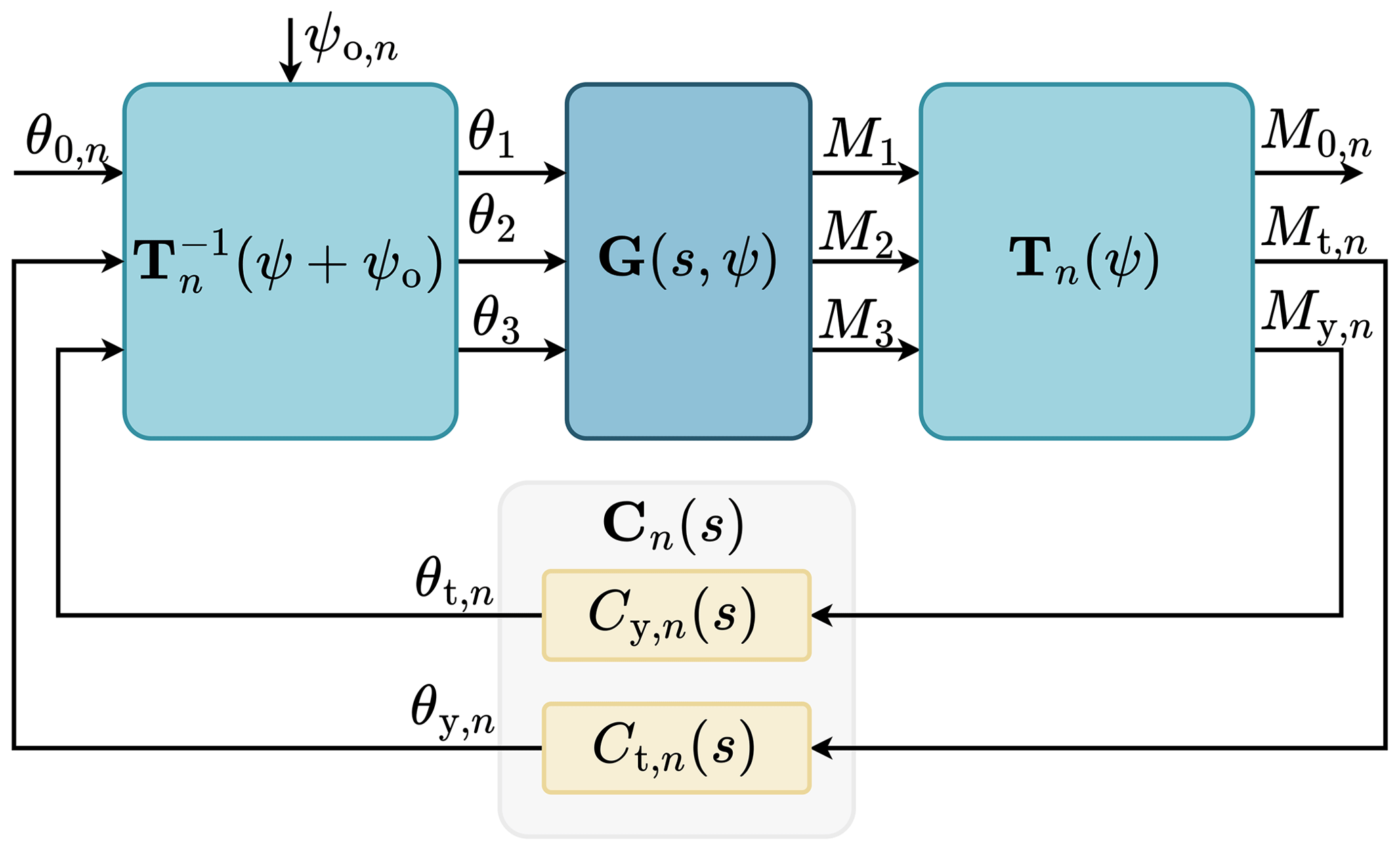
Figure 1 Block diagram of full IPC for the nP blade harmonic, fully attenuating the tilt and yaw moments. The forward MBC transformation T_n transforms the rotating blade loads to the nonrotating frame, where the SISO controllers C_t,n and C_y,n fully attenuate the tilt and yaw moments. The inverse MBC transformation ${\mathbf{T}}_n^{-\mathrm{1}}$ converts the pitch signals back to the rotating frame and includes an azimuth offset ψ_o,n to decouple the tilt and yaw axes.

If the blade load M_R contains three pure nP harmonic sine waves, M_N,n is a steady-state signal. However, due to the presence of other harmonics in the blade loads, M_N,n also contains power at 3nP harmonics. Furthermore, for unbalanced rotors, arising from load imbalance or pitch imbalance, the signal contains power at all nP harmonics (van Solingen and van Wingerden, 2015). In addition, turbulence and other stochastic effects give M_N,n power at any frequency. To focus the control loop on a single harmonic, M_N,n is usually low-pass filtered, together with a 3P notch filter (Bossanyi, 2005; van Solingen and van Wingerden, 2015), so that only the 0P contribution in the nonrotating frame, and thus the nP contribution in the rotating frame, is attenuated.

Usually, two I or PI controllers are implemented in a diagonal controller configuration, represented as

$$\begin{array}{}\text{(2)}& {\mathit{\theta }}_{\mathrm{N},n}\left(s\right)=\left[\begin{array}{ccc}\mathrm{0}& \mathrm{0}& \mathrm{0}\\ \mathrm{0}& C_{\mathrm{t},n}\left(s\right)& \mathrm{0}\\ \mathrm{0}& \mathrm{0}& C_{\mathrm{y},n}\left(s\right)\end{array}\right]{\mathit{M}}_{\mathrm{N},n}\left(s\right),\end{array}$$

where ${\mathit{\theta }}_{\mathrm{N},n}={\left[\begin{array}{ccc}{\mathit{\theta }}_{\mathrm{0},n}& {\mathit{\theta }}_{\mathrm{t},n}& {\mathit{\theta }}_{\mathrm{y},n}\end{array}\right]}^{\mathsf{T}}$ denotes the nonrotating pitch vector consisting of the collective, tilt, and yaw pitch angles of the nP harmonic in the nonrotating frame. The IPC controller is only active on the tilt and yaw channels, which relate to the oscillating part of the moments, so the first row and column are filled with zeros. These controllers fully attenuate the tilt and yaw moments by producing the necessary tilt and yaw pitch angles to drive the tilt and yaw moments to zero. In this work, we refer to this as full IPC.

These tilt and yaw pitch angles are then converted back to the rotating frame using the inverse MBC transformation, defined as

$$\begin{array}{}\text{(3)}& {\mathit{\theta }}_{\mathrm{R}}\left(t\right)={\mathbf{T}}_n^{-\mathrm{1}}\left(\mathit{\psi }\right(t)+{\mathit{\psi }}_{\mathrm{o},n}){\mathit{\theta }}_{\mathrm{N},n}\left(t\right),\end{array}$$

with

$${\mathbf{T}}_n^{-\mathrm{1}}=\left[\begin{array}{ccc}\mathrm{1}& \cos \left(n\right[{\mathit{\psi }}_{\mathrm{1}}\left(t\right)+{\mathit{\psi }}_{\mathrm{o},n}\left]\right)& \sin \left(n\right[{\mathit{\psi }}_{\mathrm{1}}\left(t\right)+{\mathit{\psi }}_{\mathrm{o},n}\left]\right)\\ \mathrm{1}& \cos \left(n\right[{\mathit{\psi }}_{\mathrm{2}}\left(t\right)+{\mathit{\psi }}_{\mathrm{o},n}\left]\right)& \sin \left(n\right[{\mathit{\psi }}_{\mathrm{2}}\left(t\right)+{\mathit{\psi }}_{\mathrm{o},n}\left]\right)\\ \mathrm{1}& \cos \left(n\right[{\mathit{\psi }}_{\mathrm{3}}\left(t\right)+{\mathit{\psi }}_{\mathrm{o},n}\left]\right)& \sin \left(n\right[{\mathit{\psi }}_{\mathrm{3}}\left(t\right)+{\mathit{\psi }}_{\mathrm{o},n}\left]\right)\end{array}\right],$$

where ${\mathit{\theta }}_{\mathrm{R}}={\left[\begin{array}{ccc}{\mathit{\theta }}_{\mathrm{1}}& {\mathit{\theta }}_{\mathrm{2}}& {\mathit{\theta }}_{\mathrm{3}}\end{array}\right]}^{\mathsf{T}}$ denotes the rotating pitch vector containing the pitch angles of the three blades defined in the rotating frame, and ${\mathit{\psi }}_{\mathrm{o},n}\in \mathbb{R}$ denotes the azimuth offset used for the nP harmonic.

2.3 Rotations in the MBC transformation

The MBC transformation can be decomposed as a Clarke transformation followed by a rotation (O'Rourke et al., 2019). Note that those authors define this rotation as the DQ0 transformation, but the DQ0 transformation is usually defined as equal to the MBC transformation.

An offset in the forward or inverse MBC transformation results in an offset in the rotation transformation and thus a rotation of the nonrotating frame. This is mathematically derived by considering the forward MBC transformation for the first harmonic with an azimuth offset ψ_o, given by

$$\begin{array}{}\text{(4)}& \begin{array}{rl}& \mathbf{T}(\mathit{\psi }+{\mathit{\psi }}_{\mathrm{o}})\\ =& {\displaystyle \frac{\mathrm{2}}{\mathrm{3}}}\left[\begin{array}{ccc}\mathrm{1}/\mathrm{2}& \mathrm{1}/\mathrm{2}& \mathrm{1}/\mathrm{2}\\ \cos ({\mathit{\psi }}_{\mathrm{1}}+{\mathit{\psi }}_{\mathrm{o}})& \cos ({\mathit{\psi }}_{\mathrm{2}}+{\mathit{\psi }}_{\mathrm{o}})& \cos ({\mathit{\psi }}_{\mathrm{3}}+{\mathit{\psi }}_{\mathrm{o}})\\ \sin ({\mathit{\psi }}_{\mathrm{1}}+{\mathit{\psi }}_{\mathrm{o}})& \sin ({\mathit{\psi }}_{\mathrm{2}}+{\mathit{\psi }}_{\mathrm{o}})& \sin ({\mathit{\psi }}_{\mathrm{3}}+{\mathit{\psi }}_{\mathrm{o}})\end{array}\right]\\ =& {\displaystyle \frac{\mathrm{2}}{\mathrm{3}}}\left[\begin{array}{ccc}\mathrm{1}& \mathrm{0}& \mathrm{0}\\ \mathrm{0}& \cos \left({\mathit{\psi }}_{\mathrm{o}}\right)& -\sin \left({\mathit{\psi }}_{\mathrm{o}}\right)\\ \mathrm{0}& \sin \left({\mathit{\psi }}_{\mathrm{o}}\right)& \cos \left({\mathit{\psi }}_{\mathrm{o}}\right)\end{array}\right]\\ & \cdot \left[\begin{array}{ccc}\mathrm{1}/\mathrm{2}& \mathrm{1}/\mathrm{2}& \mathrm{1}/\mathrm{2}\\ \cos \left({\mathit{\psi }}_{\mathrm{1}}\right)& \cos \left({\mathit{\psi }}_{\mathrm{2}}\right)& \cos \left({\mathit{\psi }}_{\mathrm{3}}\right)\\ \sin \left({\mathit{\psi }}_{\mathrm{1}}\right)& \sin \left({\mathit{\psi }}_{\mathrm{2}}\right)& \sin \left({\mathit{\psi }}_{\mathrm{3}}\right)\end{array}\right]\\ =& R\left({\mathit{\psi }}_{\mathrm{o}}\right)\mathbf{T}\left(\mathit{\psi }\right),\end{array}\end{array}$$

where R(ψ_o) is a rotation matrix rotating the nonrotating frame by ψ_o around the collective axis. A similar derivation holds for the inverse MBC transformation.

2.4 Frequency domain analysis

The MBC transformations can be transformed to the Laplace domain, enabling frequency domain analysis, useful for controller design and calibration. The main results from Lu et al. (2015) and Mulders et al. (2019) are given here. Transforming the forward transformation (Eq. 1) to the Laplace domain yields

$$\begin{array}{}\text{(5)}& {\mathcal{M}}_{\mathrm{N},n}\left(s\right)={\displaystyle \frac{\mathrm{2}}{\mathrm{3}}}{C}_{\mathrm{L},n}{\mathcal{M}}_{\mathrm{R}}\left(s_{-}\right)+{\displaystyle \frac{\mathrm{2}}{\mathrm{3}}}{C}_{\mathrm{H},n}{\mathcal{M}}_{\mathrm{R}}\left(s_{+}\right),\end{array}$$

and the inverse transformation (Eq. 3) is transformed to

$$\begin{array}{}\text{(6)}& {\mathit{\theta }}_{\mathrm{R}}\left(s\right)={\stackrel{\mathrm{̃}}{C}}_{\mathrm{L},n}^{\mathsf{T}}\left({\mathit{\psi }}_{\mathrm{o},n}\right){\mathit{\theta }}_{\mathrm{N},n}\left(s_{-}\right)+{\stackrel{\mathrm{̃}}{C}}_{\mathrm{H},n}^{\mathsf{T}}\left({\mathit{\psi }}_{\mathrm{o},n}\right){\mathit{\theta }}_{\mathrm{N},n}\left(s_{+}\right),\end{array}$$

where C_L,n and C_H,n denote the low and high partial transformation matrices for the nP harmonic, respectively; ${\stackrel{\mathrm{̃}}{C}}_{\mathrm{L},n}^{\mathsf{T}}\left({\mathit{\psi }}_{\mathrm{o},n}\right)$ and ${\stackrel{\mathrm{̃}}{C}}_{\mathrm{H},n}^{\mathsf{T}}\left({\mathit{\psi }}_{\mathrm{o},n}\right)$ denote the transpose of the partial transformation matrices including azimuth offset for the nP harmonic; and $s_{\pm }=s\pm jn{\mathit{\omega }}_{\mathrm{r}}$ and denotes the frequency-shifted Laplace operator.

By analyzing the wind turbine plant G(s,ψ) surrounded by the MBC transformations, the demodulated plant ${\stackrel{\mathrm{̃}}{\mathbf{G}}}_n\left(s\right)$ for the nP harmonic is defined, shown in Fig. 2. This demodulated plant is linear time-invariant (LTI) after averaging out the azimuth dependency, which physically makes sense since the rotating blade loads are transformed to a nonrotating frame, where the azimuth angle has no meaning (Bir, 2008). Note that the demodulated plant is depicted as a 2×2 system without the collective input θ₀ and collective output M₀ since these are not linked to the periodic loads and are not used by the individual pitch controller.

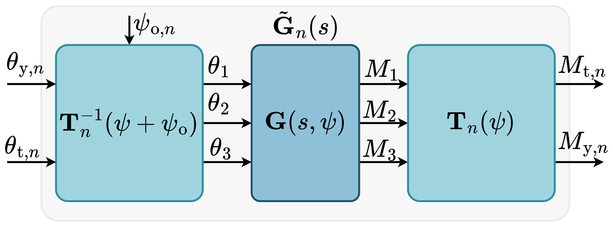
Figure 2 Block diagram of the demodulated plant ${\stackrel{\mathrm{̃}}{\mathbf{G}}}_n\left(s\right)$. By calibrating the azimuth offset ψ_o,n, the low-frequency cross-coupling from θ_t and θ_y to M_y and M_t, respectively, is minimized.

Due to dynamics in the wind turbine, there is a coupling between the tilt and yaw inputs and outputs. The system thus needs to be decoupled to enable the use of SISO controllers.

2.5 Decoupling using the optimal azimuth offset

Phase lag in the system due to, e.g., actuator dynamics, blade dynamics, dynamic induction, and communication delays, causes coupling in the nonrotating frame, leading to interactions between the tilt input and the yaw output and vice versa. Turbines with more flexible blades have slower dynamics, and thus more coupling, which must be considered during the controller design process.

The literature describes two ways to deal with this coupling. The first is to design a multivariable controller that takes the coupling into account (Bossanyi, 2003; Lu et al., 2015). Second, the system can be decoupled by using an azimuth offset in the inverse MBC transformation (Mulders et al., 2019; Mulders and van Wingerden, 2019). After the system has been decoupled, SISO controllers are used to independently control the tilt and yaw moments.

The demodulated plant ${\stackrel{\mathrm{̃}}{\mathbf{G}}}_n\left(s\right)$ is fully decoupled when its relative gain array (RGA) (Skogestad and Postlethwaite, 2010) is close to the identity. The RGA is a measure of the coupling between the inputs and outputs of a system and is defined as

$$\begin{array}{}\text{(7)}& \mathbf{R}\left(j\mathit{\omega }\right)=\mathbf{H}\left(j\mathit{\omega }\right)\circ \mathbf{H}(j\mathit{\omega }{)}^{-\mathsf{T}},\end{array}$$

where H denotes the frequency response matrix of the system, ω the frequency, and ∘ element-wise multiplication.

The azimuth offset allows the system to be decoupled in the low-frequency region and works by introducing an offset between the forward and inverse rotations, discussed in Sect. 2.3. Decoupling at low frequencies is sufficient and effective because the IPC controller is only active in this region. The optimal azimuth offset is found by minimizing the RGA of the off-diagonal components for low frequencies. In this work, the level of low-frequency coupling is defined as the highest off-diagonal element of the RGA matrix averaged over the low frequencies and is given by

$$\begin{array}{}\text{(8)}& R_{\mathit{\#}}=\underset{m\ne n}{max}\left\{{\displaystyle \frac{\mathrm{1}}{{\mathit{\omega }}_m}}\underset{\mathrm{0}}{\overset{{\mathit{\omega }}_m}{\int }}\left|{\mathbf{R}}_{m,n}\left(j\mathit{\omega }\right)\right|\mathrm{d}\mathit{\omega }\right\},m,n\in \mathit{\{}\mathrm{t},\mathrm{y}\mathit{\}},\end{array}$$

where ω_m denotes the upper limit of the low-frequency range. By selecting m and n in the set {t,y} and specifying m≠n, the off-diagonal elements from tilt to yaw and yaw to tilt are selected. The optimal azimuth offset is subsequently found by minimizing R_#.

Note that since this work focuses on the 1P blade loads, n=1. In the rest of this work, the subscript 1 is omitted for brevity. The following section uses the MBC transformation with full IPC to give an illustrative example of the trade-off between load reduction and actuator effort.

3 Illustrative example: trading off load reduction and actuator effort with conventional IPC

This section discusses controller objectives, controller calibration, and results from a conventional IPC controller. Using different controller gains, the trade-off between actuator effort and load is analyzed, similar to Han and Leithead (2015) and Lara et al. (2024) but for the IEA 15 MW turbine (Gaertner et al., 2020) at a wind speed of 15 m s⁻¹. This serves as an illustrative example of this trade-off and forms the baseline against which the proposed control methods are compared in Sect. 5.

3.1 Control objectives

This work focuses on two conflicting control objectives: fatigue load of the blade in the flapping direction and actuator effort of the pitch actuators. The fatigue load is measured through the damage equivalent load (DEL) (Sutherland, 1999; Thomsen, 1998) and is defined as

$$\begin{array}{}\text{(9)}& \text{DEL}={\left({\displaystyle \frac{\sum n_i{R}_i^m}{n_{\mathrm{eq}}}}\right)}^{\mathrm{1}/m},\end{array}$$

where n_i denotes the number of cycles at load level i; R_i the load range at load level i; n_eq the number of cycles at the equivalent load level; and m the slope of the S–N curve (or Wöhler slope), typically 10 for composites used for the blade (Zahle et al., 2024). A rainflow-counting algorithm (E08 Committee, 2017) is used to obtain n_i and R_i from a flapping moment signal. The DEL is then calculated for a certain number of cycles n_eq, which is typically set to the simulation length to calculate the DEL for a 1 Hz equivalent load. The objective in this work is the flapping moment DEL and is calculated by averaging the flapping moment DEL for each of the three blades.

The actuator effort is evaluated using the actuator duty cycle (ADC) (Bottasso et al., 2013), which represents the normalized total travel angle and is defined as

$$\begin{array}{}\text{(10)}& \text{ADC}={\displaystyle \frac{\mathrm{1}}{T}}\underset{\mathrm{0}}{\overset{T}{\int }}\left|{\displaystyle \frac{\dot{u}\left(t\right)}{{\dot{u}}_{\max }}}\right|\mathrm{d}t,\end{array}$$

where $\dot{u}\left(t\right)$ is the time derivative of the control input, ${\dot{u}}_{\max }$ is the maximum control input rate, and T is the duration over which the ADC is calculated. To calculate the ADC for the wind turbine, the pitch rate is used as the control input, and the average ADC is calculated for the three pitch signals. Furthermore, ${\dot{u}}_{\max }$ is set to 2° s⁻¹, which is the maximum pitch rate of the IEA 15 MW wind turbine (Gaertner et al., 2020).

3.2 Controller calibration

This section establishes a properly tuned full-IPC controller. Two control variables need to be calibrated, namely the azimuth offset used to decouple the plant and the integrator gain of the IPC controllers.

Using the procedure outlined in Sect. 2.5 of minimizing the highest off-diagonal RGA using the frequency response obtained from a spectral estimate, the optimal azimuth offset for the IEA 15 MW reference turbine at a wind speed of 15 m s⁻¹ is found to be 24.5°. Figure 3 shows the diagonal and off-diagonal frequency response of the demodulated plant with and without this azimuth offset. The off-diagonal frequency response, in the lower subplot, is significantly reduced at low frequencies when using the optimal azimuth offset, effectively decoupling the system at frequencies where the IPC controllers are active. The response on the diagonal is increased slightly by a few dB. Note that the tilt-to-tilt and the yaw-to-yaw responses are almost identical, so the tilt-to-tilt response is shown as the diagonal element. Similarly, the tilt-to-yaw and yaw-to-tilt response are almost identical, and the tilt-to-yaw response is shown as the off-diagonal element.

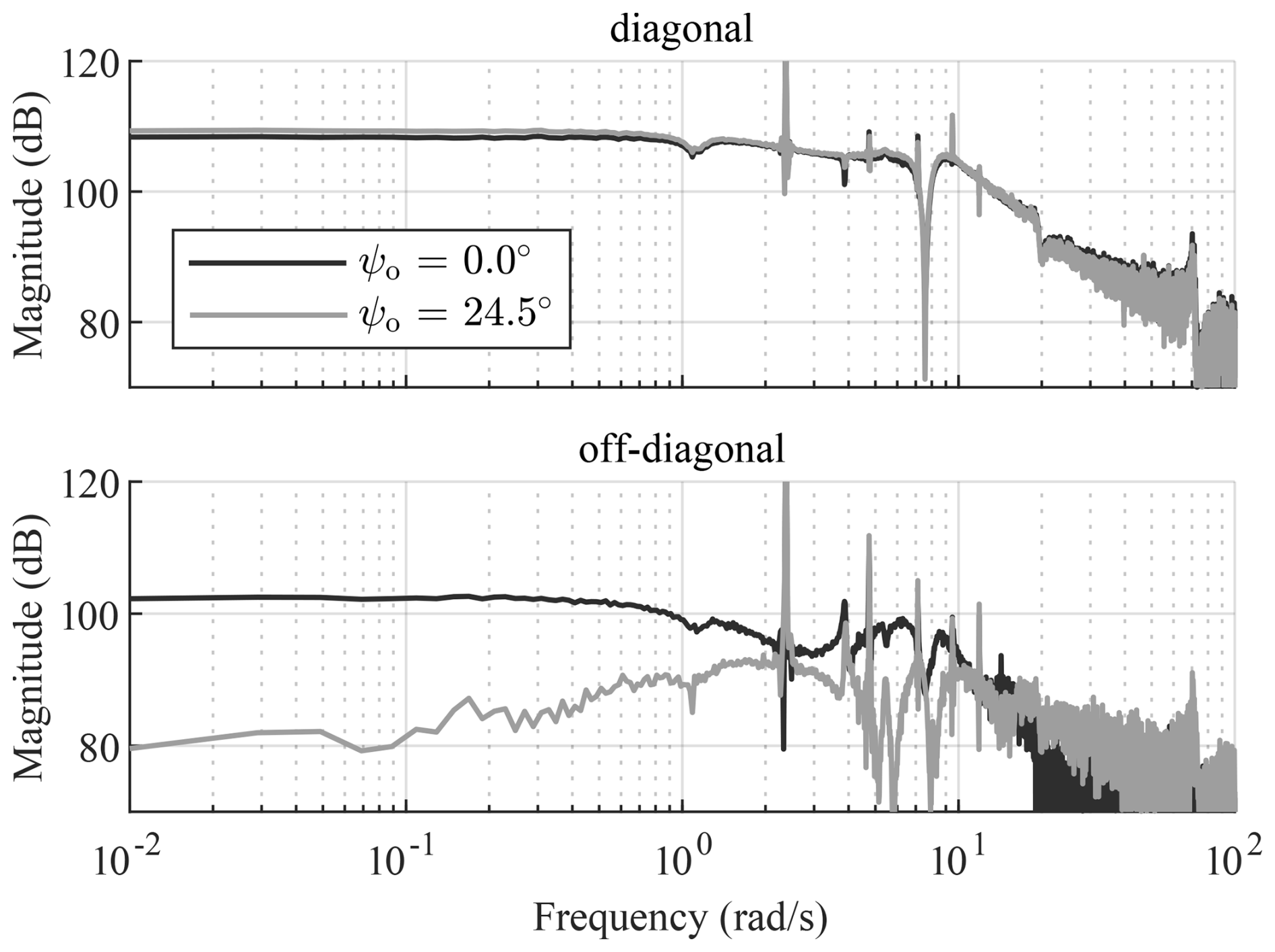
Figure 3 Frequency response of the demodulated plant with and without the optimal azimuth offset of 24.5° at a wind speed of 15 m s⁻¹. When including the azimuth offset, the off-diagonal gain is significantly reduced at low frequencies, effectively decoupling the system at those frequencies.

The diagonal controller, consisting of a tilt and a yaw controller, uses the same gain for both controllers since the diagonals of the decoupled demodulated plant are almost identical. This work assumes a pure I controller that targets a certain open-loop crossover frequency. A grid search is performed to assess the effect of the crossover frequency on the trade-off between DEL and ADC. The minimum crossover frequency is set to 0.01 rad s⁻¹, which corresponds to a time constant of 100 s. At this time constant, the controller would converge to 95 % of its steady-state value in 300 s, which is the same amount of time that we discard in the simulation to let the turbine reach steady state. Even slower controllers would take longer to converge, making their simulation and thus analysis impractical. The maximum crossover frequency is set to 1.25 rad s⁻¹, at which point the stability margins are significantly reduced and performance degrades.

3.3 Results

Using OpenFAST (Jonkman et al., 2023), simulations were run on the IEA 15 MW reference turbine (Gaertner et al., 2020) in monopile configuration. All degrees of freedom were enabled, but hydrodynamic loads were disabled to focus on the oscillating blade loads induced by wind shear. The simulations were run at a wind speed of 15 m s⁻¹, so the turbine operates in above-rated conditions with a constant torque and a collective pitch controller implementation from ROSCO (Abbas et al., 2022, 2024) to regulate the rotor speed. A vertical wind shear coefficient of 0.07 with a power law profile was chosen to represent realistic offshore conditions (Yang et al., 2024). Both laminar and turbulent conditions were tested. Each wind condition was run with nine different integrator gains to assess the effect of controller tuning.

Figure 4 shows the results for laminar wind conditions. All full-IPC controllers converge to the same steady-state operating point, and the bandwidth of the controller, as expected in laminar conditions, does not affect this. The 1P oscillating load is always completely attenuated since the DC gain of the demodulated plant's diagonal open-loop transfer functions is infinite due to the use of an integral control element. This means that the tilt and yaw moments are fully attenuated by significantly pitching the blades and that the controller tuning does not affect the trade-off between DEL and ADC. So there are two options: no IPC with a high fatigue load and low actuator effort or full IPC (with any stable tuning) with a lower fatigue load and higher actuator effort.

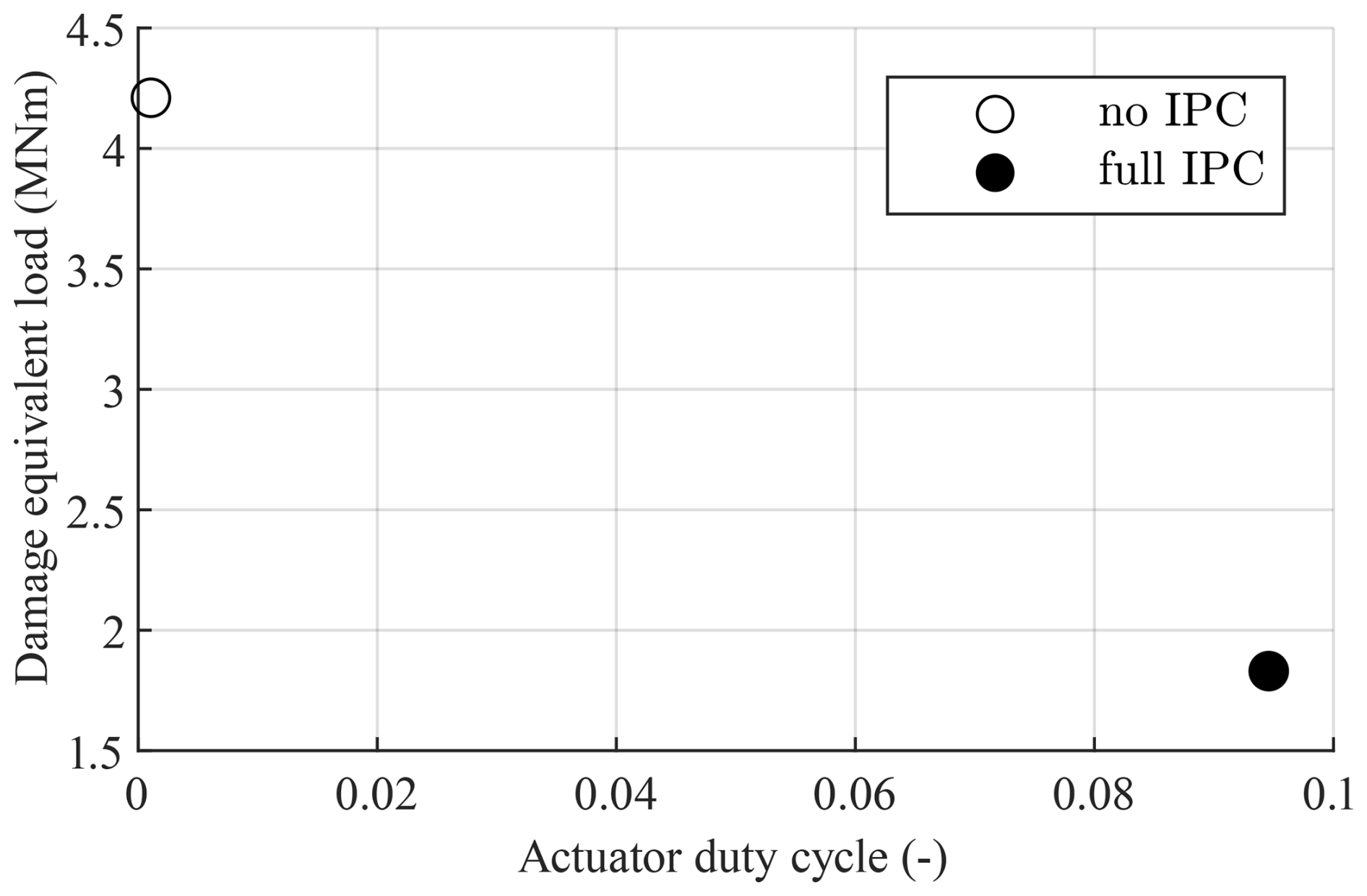
Figure 4 Trade-off between DEL and ADC for full IPC in laminar wind conditions. Controller tuning has no effect since the controllers reach a steady-state operating condition. So the only trade-off is to turn IPC on or off.

In turbulent wind conditions, the controller constantly adapts to changing wind conditions, so the bandwidth of the controller affects its performance. The turbulent wind fields are generated using TurbSim (Jonkman, 2009) using the IECKAI turbulence model with 8 % turbulence intensity. To obtain statistically significant results, each controller tuning was run for 10 different instances of turbulence using a different input seed for TurbSim. Furthermore, each simulation was run for 2100 s, resulting in 30 min of valid data per simulation after discarding the first 300 s to eliminate initialization effects.

Over these 30 min, the DEL and ADC for each controller gain were calculated and are shown in Fig. 5. With no IPC action, there is a high damage equivalent load but little actuator effort. The actuator effort is not equal to zero since the collective pitch control is active and regulates the rotor speed in these turbulent conditions. Furthermore, the fatigue load is higher than in laminar conditions due to the additional excitation of the blades. Full IPC with different gains results in different trade-offs between DEL and ADC. The highest reduction in load is achieved when targeting a crossover frequency of 0.75 rad s⁻¹, and the controllers with a higher bandwidth increase the DEL while also increasing the actuator effort. The controllers with a higher bandwidth achieve a smaller mean error in tilt and yaw but with a higher variance. This is because the stability margins have been reduced. These additional oscillations ultimately increase the DEL. With the lowest bandwidth, the controllers get closer to no IPC, but to get even closer, the time constant would have to be set unreasonably large. Instead of making this trade-off with controller tuning, output-constrained IPC makes this trade-off by setting a reference load. Two such methods are introduced next and compared to this result in Sect. 5.

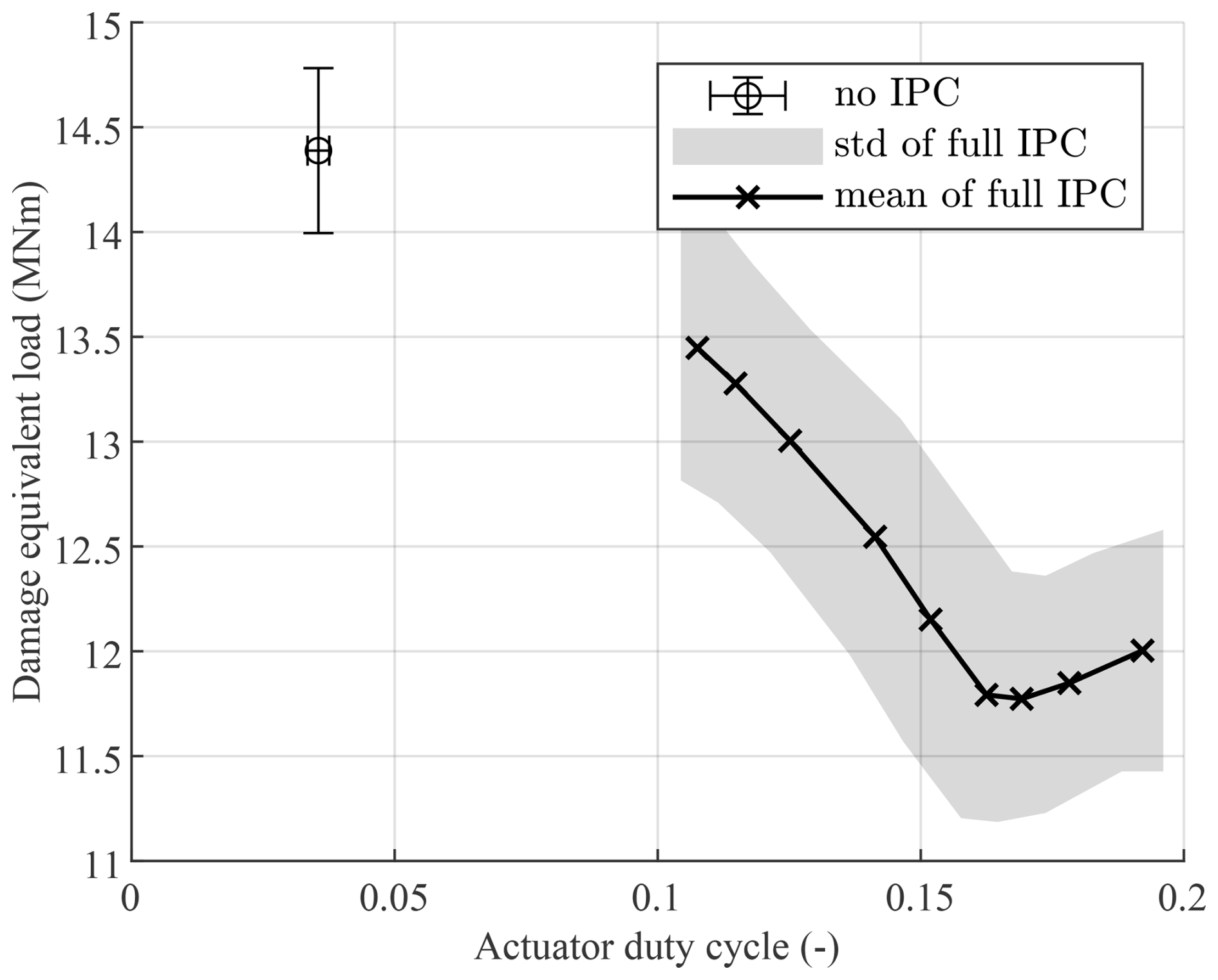
Figure 5 Trade-off between DEL and ADC with 8 % turbulence intensity averaged over 10 turbulent wind field instances. The error bars for no IPC and the shaded area for full IPC indicate the standard deviation (1σ), resulting from the different turbulent seeds. The full-IPC controller was tested with a crossover frequency of between 0.01 and 1.25 rad s⁻¹. For a crossover frequency of 0.75 rad s⁻¹, the full-IPC controller has the highest reduction in DEL. Increasing the gains leads to reduced stability margins, which leads to more oscillations and thus an increase in DEL. Reducing the gain brings the trade-off closer to no IPC. However, lowering the gain too much results in time constants larger than 100 s, so the full-IPC controller cannot make the complete trade-off.

4 Output-constrained individual pitch control using the multiblade coordinate transformation

Full IPC drives the oscillating loads to zero. Output-constrained IPC instead drives the loads to some reference value. When using the MBC transformation, the tilt and yaw moments are thus driven to some reference. This section defines two types of references through the norm they represent and subsequently proposes two output-constrained IPC methods using the MBC transformation, namely ℓ^∞ IPC and ℓ² IPC. It will become apparent that both methods require an estimation of the open-loop load, which is defined as the load that the system would experience without any IPC action, which is also derived.

4.1 Load norms

Using the MBC transformation, the oscillating load is decomposed in a tilt and a yaw contribution. These contributions are visualized using a vector in a tilt–yaw plane, shown in Fig. 6. Full IPC drives this tilt–yaw moment vector to the origin, fully attenuating the 1P oscillating load. Output-constrained IPC instead drives this vector to a certain reference or constrains the norm of this load vector to a certain value.

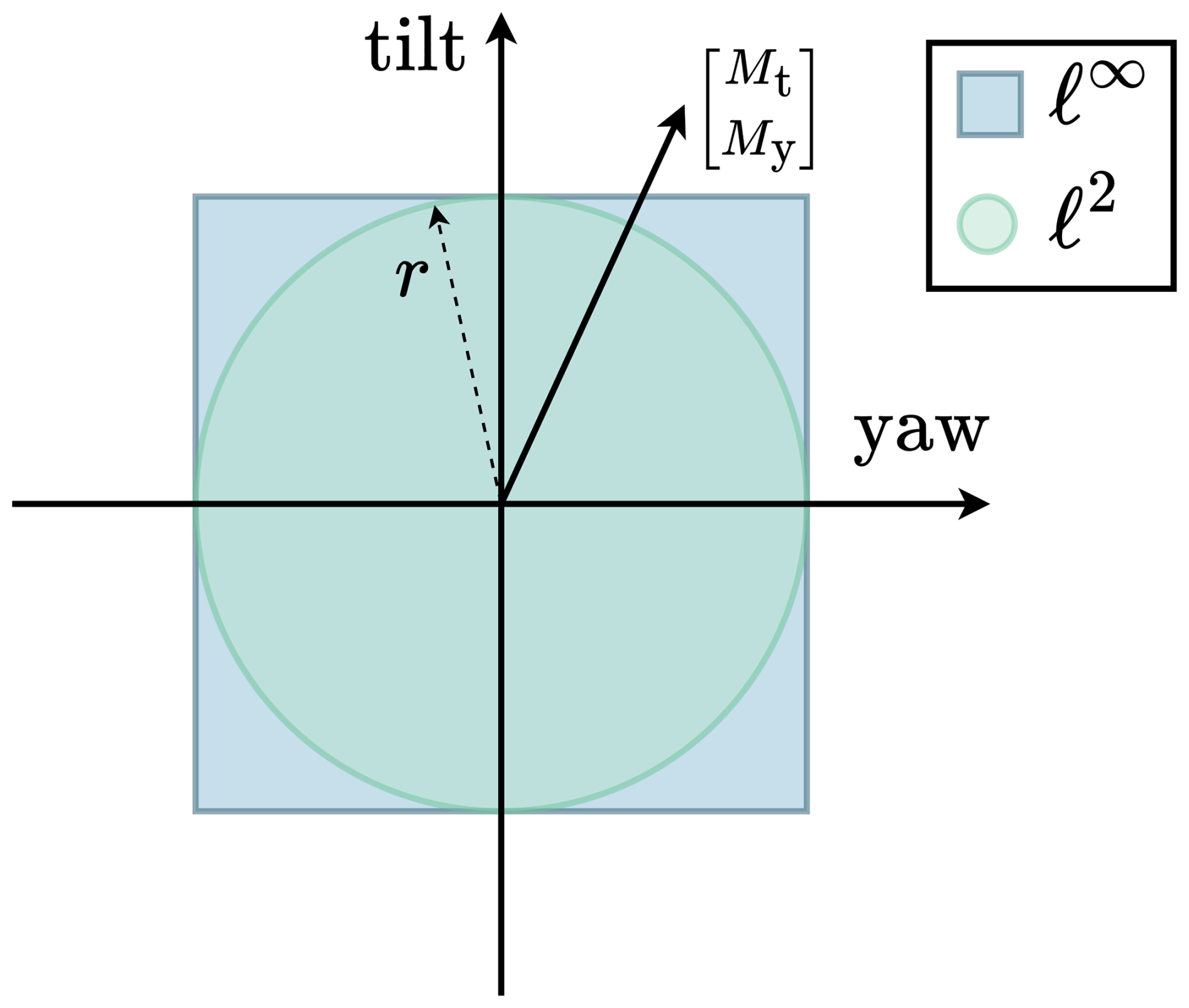
Figure 6 The tilt and yaw moments are visualized as a vector on the tilt–yaw plane. Output-constrained IPC then constrains this vector to a reference r. Shown here are the ℓ^∞ and ℓ² norms to constrain the load, which form the fundament of the ℓ^∞ IPC and ℓ² IPC methods.

In this work, the load is constrained using two different norms, the ℓ^∞ and ℓ² norms, both defined through the p norm:

$$\begin{array}{}\text{(11)}& {∥\left[\begin{array}{c}{M}_{\mathrm{t}}\\ M_{\mathrm{y}}\end{array}\right]∥}_p=\sqrt[p]{M_{\mathrm{t}}^p+M_{\mathrm{y}}^p}.\end{array}$$

For p=∞, this norm equals the infinity norm, resulting in a square reference, and for p=2, this norm equals the Euclidian norm, resulting in a circular reference, both shown in Fig. 6.

4.2 ℓ^∞ IPC

Using the ℓ^∞ norm of the load vector, the controller behaves in a decoupled manner and drives the tilt moment to a tilt reference r_t and the yaw moment to a yaw reference r_y, as shown in Fig. 7. It uses the decoupling between the tilt and yaw axes to use independent tilt and yaw controllers, defined as

$$\begin{array}{}\text{(12)}& C_{\mathrm{t}}\left(s\right)=C_{\mathrm{y}}\left(s\right)={\displaystyle \frac{K_{\mathrm{i}}}{s}},\end{array}$$

where K_i is the integral gain.

This method was hypothesized in the introduction of Liu et al. (2022) as a “deadband” augmentation of conventional IPC and is an extension of Henry et al. (2024) by adding a yaw reference and the ability for the references to be both positive and negative.

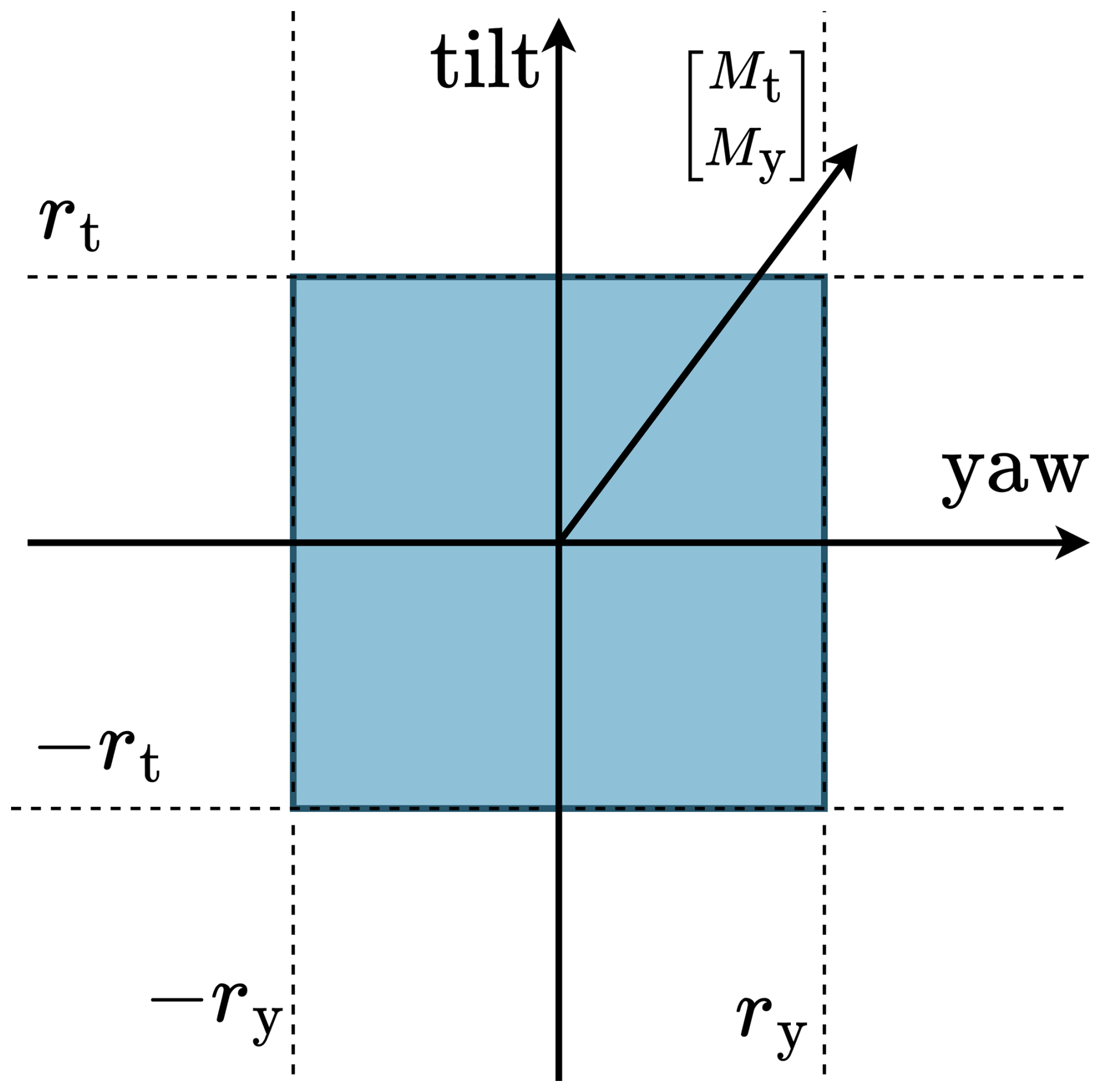
Figure 7 Using ℓ^∞ IPC, the nonrotating load vector is independently driven to a tilt and yaw reference r_t and r_y. The load is thus constrained within an ℓ^∞ norm, indicated by a square.

The negative reference on the tilt axis is likely not often active. However, it may become necessary when the wind conditions have a negative shear component, which does occur sometimes, especially offshore (Yan et al., 2022).

There are two main challenges with this approach. First, the tilt and yaw moments should never be amplified to the reference because the control objective is load reduction, not amplification. In closed loop, when the controller drives the moment to a certain reference, the measurement of this moment alone is insufficient information to determine whether this load has been amplified or reduced to its current value. Second, the sign of the reference should be changed appropriately since the load vector can take any value in the tilt–yaw plane and can therefore switch signs. Similarly, once the closed-loop system is at a certain load, measuring the moments alone is insufficient information to determine whether the positive or negative reference should be used.

Both of these problems are solved by estimating the “open-loop load”, which is defined as the load in the tilt–yaw plane that the system would experience in open loop, so when the output-constrained IPC controller is disengaged. The derivation of the open-loop load estimator is discussed in Sect. 4.4.

If the original tilt moment is positive, the tilt moment will be constrained between its current value and zero. So a positive tilt reference is selected. Furthermore, the tilt controller is saturated on [0,∞), preventing the tilt moment from increasing so that the load is kept constant or reduced towards zero. If the reference is between the original tilt load and zero, the load is driven towards the reference, but if the reference is above the original tilt load, the controller is saturated and no IPC action is done. In contrast, if the original tilt moment is negative, the negative tilt reference is selected and the tilt controller is saturated on $(-\mathrm{\infty },\mathrm{0}]$; this allows the controller to increase the tilt moment, bringing any negative moment closer to the origin. The same logic applies to the yaw channel.

Figure 8 shows the block diagram for the ℓ^∞ IPC method. The tilt and yaw moments, together with the tilt and yaw pitch angles, are used to estimate the open-loop load. The sign of the original tilt moment is then used to set the sign of the tilt reference and select the saturation bounds for the tilt controller based on the logic mentioned previously. The same applies to the yaw channel. Overall, the tilt and yaw channels remain decoupled in this approach, and each channel either drives the load to its reference or is saturated to avoid amplification.

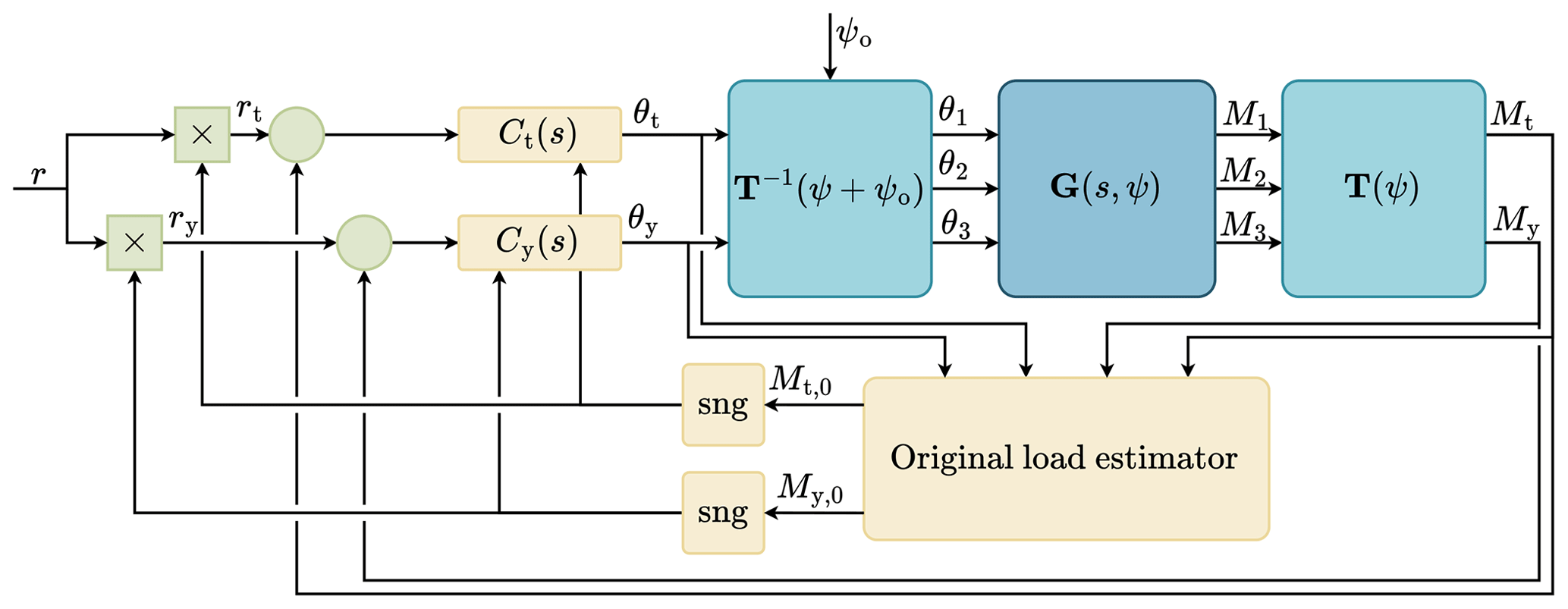
Figure 8 Block diagram of ℓ^∞ IPC. It uses a decoupled tilt and yaw controller that both drive the moment to the reference. To avoid load amplification, the reference sign and integrator saturation are adjusted based on the sign of the open-loop load.

This approach is robust to modeling errors in the open-loop load estimation because only information about its sign is used. As long as the sign of the open-loop load is estimated correctly, the controller will saturate its control signal in the correct direction and select the correct sign of the reference load. However, when the sign of the open-loop estimate changes and the current tilt or yaw pitch angle is not zero, a step change in the commanded pitch angle will occur. This effect would be reduced through the actuator dynamics but is neglected in this work.

4.3 ℓ² IPC

Instead of constraining the tilt and yaw loads separately, using the ℓ² norm of the nonrotating load vector, the magnitude of the load is constrained. This is achieved by projecting the nonrotating load vector to a new reference frame, where the magnitude of the load is projected on a single axis, as shown in Fig. 9. The new reference frame consists of a radial and a tangential component. In steady state, the magnitude of the load is projected on the radial axis and the tangential component would be zero. This allows a single controller, defined as

$$\begin{array}{}\text{(13)}& C_{\mathrm{r}}\left(s\right)={\displaystyle \frac{K_{\mathrm{i}}}{s}},\end{array}$$

which acts on the radial axis to directly regulate the magnitude of the load. Note that the integral gain K_i is equal to the integral gain of the ℓ^∞ IPC method to provide a fair comparison. The rotation of this axis system is achieved using the rotations inherent to the MBC transformation, as previously discussed in Sect. 2.3. The rotation is done by angle ψ_r.

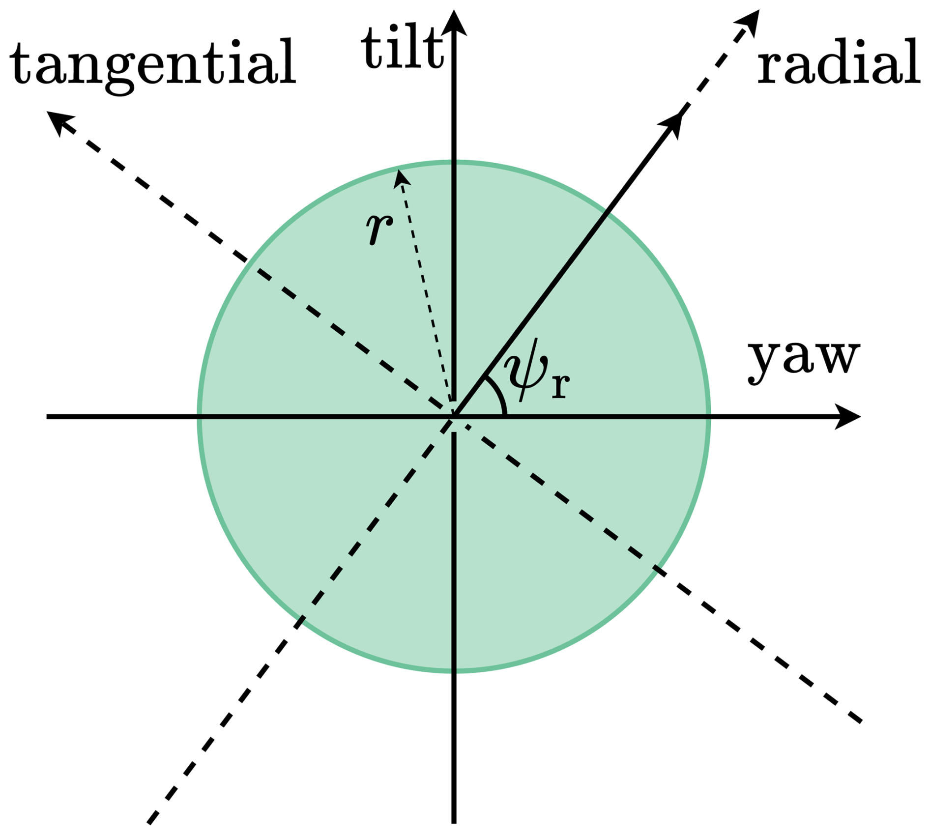
Figure 9 Using ℓ² IPC, the nonrotating load vector is projected on a new orthogonal reference system, consisting of a radial and tangential axis. In this new axis system, the magnitude of the load is projected on the radial axis. The load is thus constrained using the ℓ² norm, indicated by a circle.

This means that the nonrotating pitch angles are in phase with the nonrotating load. This is ideal when the azimuth offset in the inverse transformation ensures that the phase lag from the nonrotating pitch to the nonrotating moment is zero. While the optimal azimuth offset is defined to achieve decoupling, it also causes an almost zero phase shift from the nonrotating pitch to the nonrotating moment.

Ensuring that the controller does not amplify the loads is more straightforward than for the ℓ^∞ IPC method. Since the controller only acts on the magnitude, which is always positive, it should only lower the magnitude of the load, which is achieved by saturating the controller on [0,∞).

The challenge lies in estimating the rotation ψ_r and its estimation bandwidth. It can be estimated by taking the inverse tangent of the tilt and yaw moment. However, when operating close to full IPC, these moments are reduced to zero, making this estimate noisy, or worse, undefined. As a solution, the ℓ² IPC method also uses the estimate of the open-loop load for ψ_r, which is thus calculated as

$$\begin{array}{}\text{(14)}& {\mathit{\psi }}_{\mathrm{r}}=\mathrm{atan}\mathrm{2}\left(M_{\mathrm{t},\mathrm{o}},M_{\mathrm{y},\mathrm{o}}\right),\end{array}$$

where M_t,o and M_y,o are the original tilt and yaw moments, respectively, whose estimation is discussed in Sect. 4.4. This ensures that a robust estimate of the rotation angle is obtained even when operating close to full IPC (and the measured load is close to zero).

The angle ψ_r is effectively the phase of the final commanded pitch angles to the three blades. This phase should thus change sufficiently quickly to adapt to changes in wind conditions but should not contain noise as it directly translates to noise in the phase of the pitch signal.

Figure 10 shows the block diagram of ℓ² IPC. Similarly to ℓ^∞ IPC, the open-loop load estimator uses the nonrotating moments and pitch angles. The angle of the open-loop load in the tilt–yaw plane is then calculated and used to rotate the tilt and yaw moment to a new reference system with a radial and a tangential component. The inverse rotation uses the same angle to rotate the radial control action back to a tilt and yaw component. This control method only needs a single controller, C_r(s), to regulate the radial moment to a reference because it actuates in the ideal phase. This is in contrast to conventional IPC and ℓ^∞ IPC, which control the tilt and yaw axes separately and thus need two controllers.

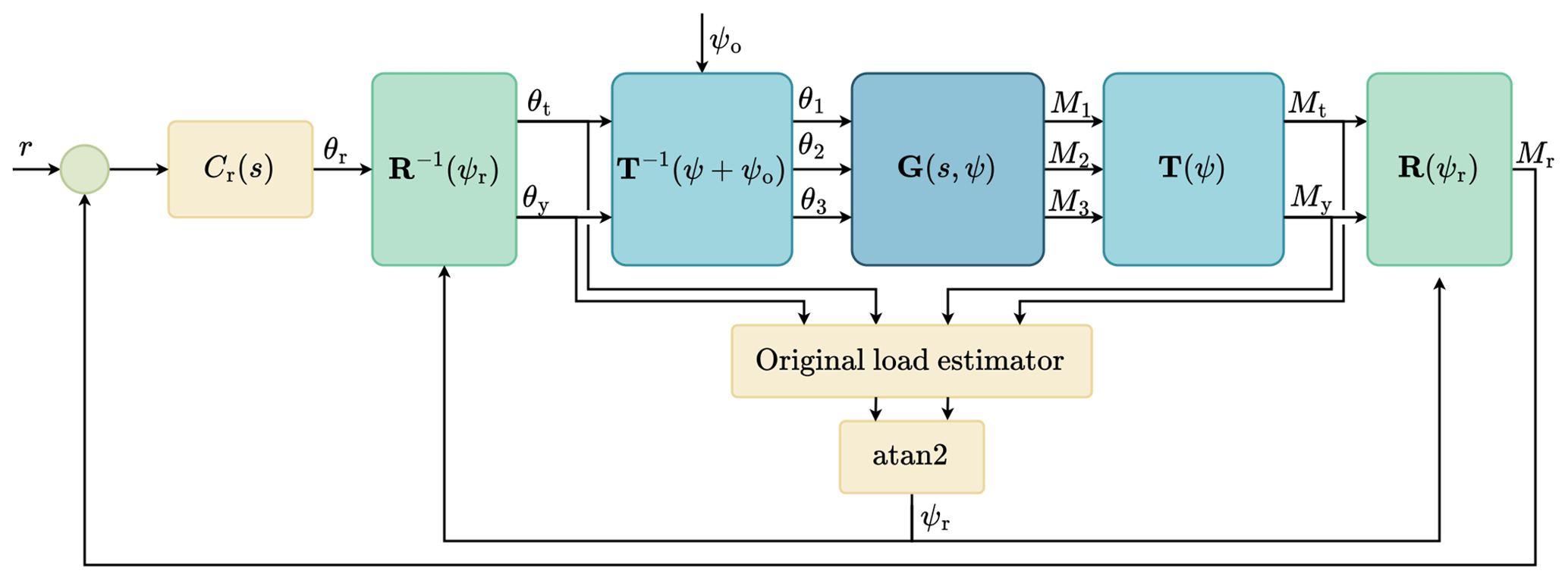
Figure 10 Block diagram of ℓ² IPC. The open-loop load estimator uses the nonrotating loads and nonrotating pitch angles to reconstruct the open-loop load. The angle of this load in the tilt–yaw plane is ψ_r, which is used to rotate the reference system to a radial and tangential axis where the magnitude of the nonrotating load vector is projected on the radial axis. A single SISO controller then regulates this load magnitude.

4.4 Open-loop load estimation

The open-loop load is the load experienced by the system if IPC were disengaged. In closed loop, with IPC active, this cannot be measured and should instead be estimated. The estimation consists of a measurement of the current load and an estimation of the load that is regulated away with the current IPC action, using a simple model.

In steady state, and by using a first-order approximation, the open-loop load is defined as

$$\begin{array}{}\text{(15)}& {\mathit{M}}_{\mathrm{N},\mathrm{o}}={\mathit{M}}_{\mathrm{N}}-{\mathbb{J}}_{{\mathit{M}}_{\mathrm{N},\mathrm{o}}}{\mathit{\theta }}_{\mathrm{N}},\end{array}$$

with

$${\mathbb{J}}_{{\mathit{M}}_{\mathrm{N},\mathrm{o}}}=\left[\begin{array}{ccc}\frac{\partial M_{\mathrm{0}}}{\partial {\mathit{\theta }}_{\mathrm{0}}}& \frac{\partial M_{\mathrm{0}}}{\partial {\mathit{\theta }}_{\mathrm{t}}}& \frac{\partial M_{\mathrm{0}}}{\partial {\mathit{\theta }}_{\mathrm{y}}}\\ \frac{\partial M_{\mathrm{t}}}{\partial {\mathit{\theta }}_{\mathrm{0}}}& \frac{\partial M_{\mathrm{t}}}{\partial {\mathit{\theta }}_{\mathrm{t}}}& \frac{\partial M_{\mathrm{t}}}{\partial {\mathit{\theta }}_{\mathrm{y}}}\\ \frac{\partial M_{\mathrm{y}}}{\partial {\mathit{\theta }}_{\mathrm{0}}}& \frac{\partial M_{\mathrm{y}}}{\partial {\mathit{\theta }}_{\mathrm{t}}}& \frac{\partial M_{\mathrm{y}}}{\partial {\mathit{\theta }}_{\mathrm{y}}}\end{array}\right],$$

which is the Jacobian of the nonrotating blade moments with respect to the nonrotating blade pitch angles and is equal to the steady-state gain of $\stackrel{\mathrm{̃}}{\mathbf{G}}\left(s\right)$. This estimate thus requires model information, which can be obtained through system identification or linearizations of a wind turbine model. Note that while this definition also includes the estimate of the original collective moment, only the original tilt and yaw moments are used by the ℓ^∞ IPC and ℓ² IPC methods.

Furthermore, due to the decoupling using the azimuth offset, the off-diagonal elements of ${\mathbb{J}}_{{\mathit{M}}_{\mathrm{N},\mathrm{o}}}$ are much smaller than the diagonal elements. So, similarly to the control, the estimation of the tilt and yaw open-loop load is decoupled. This simplifies the estimation to

$$\begin{array}{}\text{(16)}& \begin{array}{rl}{\displaystyle }{M}_{\mathrm{t},o}=& {\displaystyle }{M}_{\mathrm{t}}-{\displaystyle \frac{\partial M_{\mathrm{t}}}{\partial {\mathit{\theta }}_{\mathrm{t}}}}{\mathit{\theta }}_{\mathrm{t}},\\ {\displaystyle }{M}_{\mathrm{y},o}=& {\displaystyle }{M}_{\mathrm{y}}-{\displaystyle \frac{\partial M_{\mathrm{y}}}{\partial {\mathit{\theta }}_{\mathrm{y}}}}{\mathit{\theta }}_{\mathrm{y}}.\end{array}\end{array}$$

The two partial derivatives, $\partial M_{\mathrm{t}}/\partial {\mathit{\theta }}_{\mathrm{t}}$ and $\partial M_{\mathrm{y}}/\partial {\mathit{\theta }}_{\mathrm{y}}$, are almost equal to each other. This is also why the diagonal pitch controller can have the same gains for its tilt and yaw controller.

This estimate of the open-loop load is a steady-state estimate and thus neglects the dynamics in the system. It is an instantaneous estimation of the open-loop load after transient effects have died out. To reduce the bandwidth of this estimate and filter out high-frequency components, the estimate is filtered with a low-pass filter with a cutoff frequency of ω_o. This ensures that for the ℓ^∞ IPC controller, the switching between reference sign and integrator saturation is smooth and that for the ℓ² IPC controller, no noise is introduced into the phase of the resulting sinusoidal pitch signal.

Furthermore, it is assumed that the Jacobian is constant around a certain operating condition and does not change as a function of the load reference. When using the estimator at more wind speeds, it would need to be gain-scheduled since $\partial M_{\mathrm{t}}/\partial {\mathit{\theta }}_{\mathrm{t}}$ and $\partial M_{\mathrm{y}}/\partial {\mathit{\theta }}_{\mathrm{y}}$ change with wind speed. These two proposed output-constrained IPC controllers are tested and compared against the baseline in the following section.

5 Results

This section presents the results of the ℓ^∞ IPC and ℓ² IPC methods and compares them to the baseline set in Sect. 3. It also uses the same setup with the IEA 15 MW turbine, a wind speed of 15 m s⁻¹, and a vertical shear coefficient of 0.07 (unless explicitly stated otherwise) in both laminar and turbulent conditions.

After controller calibration, four different cases are analyzed. First, in laminar wind conditions, a staircase response is shown to analyze the working mechanisms of the two control methods. Second, the trade-off between the damage equivalent load of the flapping moment and actuator duty cycle is analyzed in laminar wind conditions. Third, the controllers are tested in a wind field with changing shear coefficients to analyze the effectiveness of using the estimated open-loop load for integrator saturation and reference sign selection for ℓ^∞ IPC and phase estimation for ℓ² IPC. Lastly, both control methods were tested in turbulent wind conditions with multiple seeds to analyze the trade-off between damage equivalent load and actuator duty cycle in realistic wind conditions.

5.1 Controller calibration

The proposed output-constrained ℓ^∞ IPC and ℓ² IPC methods have the same variables that need to be calibrated, namely the azimuth offset, the integral gain for the IPC controller (C_t(s) and C_y(s) for the ℓ^∞ IPC controller and C_r(s) for the ℓ² IPC controller), and the bandwidth and partial derivatives in the open-loop load estimator. For a fair comparison, both control methods use the same calibration.

The optimal azimuth offset of 24.5°, calculated in Sect. 3.2, is also used for ℓ^∞ IPC and ℓ² IPC. In Sect. 3.3, a grid search was performed for different crossover frequencies for full IPC. For the ℓ^∞ IPC and ℓ² IPC methods, a crossover frequency of 0.2 rad s⁻¹ is selected since the full-IPC controller with this crossover frequency has a good trade-off between DEL and ADC, resulting in an integral gain $K_{\mathrm{i}}=-\mathrm{6.8}\times {\mathrm{10}}^{-\mathrm{7}}$ for C_t(s), C_y(s), and C_r(s). Note that the controller gain is negative, while in conventional IPC controllers it is positive. This is because the pitch controllers of ℓ^∞ IPC and ℓ² IPC actuate based on the load errors rather than the load itself; in other words, they use a negative feedback loop.

The bandwidth of the open-loop load estimator is set to 2 rad s⁻¹. This allows for good noise suppression while simultaneously being fast enough to respond to changes in wind shear.

The partial derivatives in the open-loop load estimator are estimated from the spectral estimate, also used to find the optimal azimuth offset. The tilt-to-tilt contribution, $\partial M_{\mathrm{t}}/\partial {\mathit{\theta }}_{\mathrm{t}}$, and the yaw-to-yaw contribution, $\partial M_{\mathrm{y}}/\partial {\mathit{\theta }}_{\mathrm{y}}$, are both equal to 109.3 dB.

5.2 Staircase response in laminar wind

The first case simulates the response of the controller in laminar conditions to analyze the working principles of the controllers and compare them. A staircase input on the reference is used to let the controller pass through different operating points between no IPC and full IPC. The reference load starts above the open-loop load, resulting in no IPC action from the output-constrained IPC controllers. It then steps to zero in four steps, each lasting 25 s, until the output-constrained IPC controllers perform equal to full IPC with a reference load of 0 N m. The first 300 s is discarded to allow the system to reach a steady state and thus exclude initialization effects.

Note that the reference for the ℓ^∞ IPC method is adjusted such that it achieves the same resultant load magnitude as the ℓ² IPC method.

Figure 11 shows the time domain results in the rotating frame of the flapping moment, 1P filtered flapping moment, and pitch signal. The 1P filtered signal is obtained by filtering the flapping moment with a finite impulse response (FIR) bandpass filter with a passband between 0.75P and 1.25P. In the first subplot, the flapping moment initially shows a strong 1P component due to wind shear, and the effect of tower shadow is also clearly visible. As the reference is reduced, the 1P component diminishes until the dominant oscillation is the 2P component. Furthermore, a small difference is observed between ℓ^∞ IPC and ℓ² IPC, which is discussed more extensively later. In the second subplot, the peaks of the 1P flapping moment of the two output-constrained IPC methods track the reference accurately. Crucially, the oscillation is not amplified towards the reference at the start of the simulation, showing that the output-constrained IPC methods only activate when the load is above the reference. However, a small difference in phase between the two control methods can be observed. The third subplot also shows this phase shift in the pitch signal. In addition, the ℓ^∞ IPC method requires a slightly larger pitch magnitude to track the same reference as ℓ² IPC. This occurs because the ℓ^∞ IPC method uses control effort to change both the magnitude and the phase of the load rather than only the magnitude.

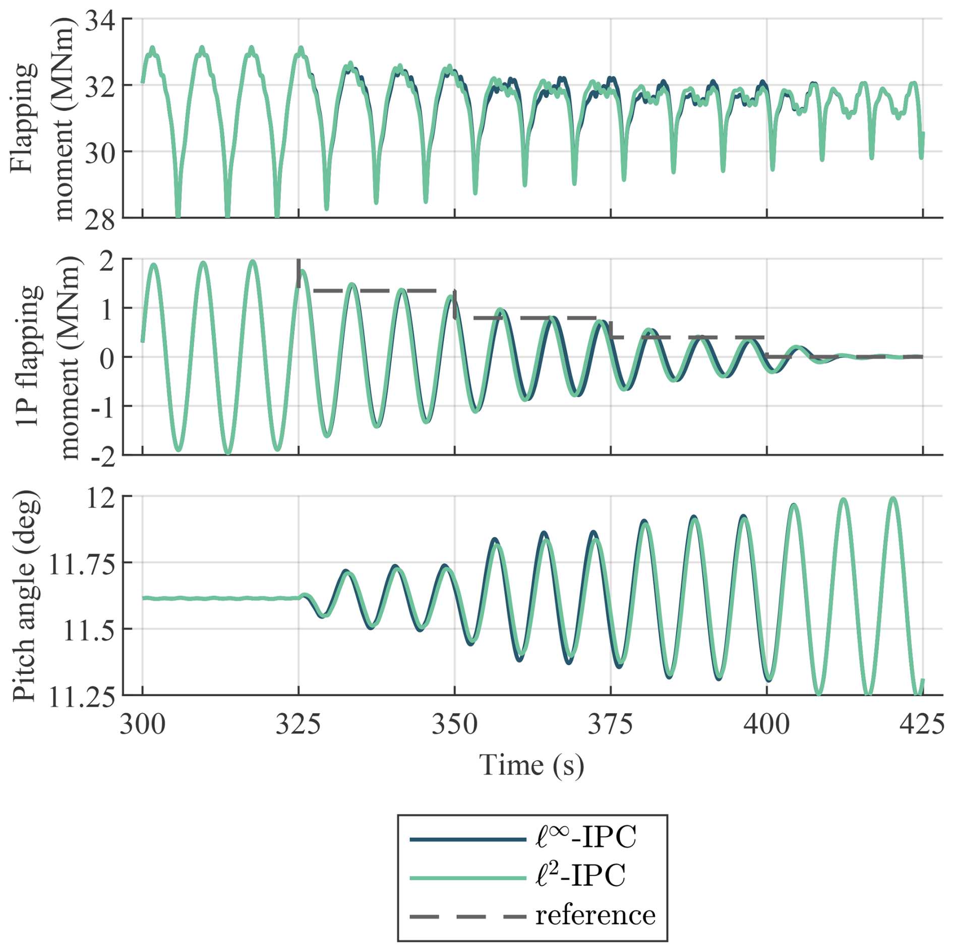
Figure 11 Time domain results to the staircase reference load input in the rotating frame. While both output-constrained IPC methods follow the reference accurately, they have a slightly different control action and resulting flapping moment during the transition between no IPC to full IPC.

The difference in control magnitude is more clearly visible in the nonrotating frame. Figure 12 shows the time domain results in the nonrotating frame of the nonrotating moment and nonrotating pitch angle. The three blade loads are transformed to the nonrotating frame using the MBC transformation and are low-pass filtered. The controllers are compared by analyzing the magnitude of the tilt and yaw contribution of the nonrotating moment and pitch angle. Both controllers track the reference accurately and have a similar transient response due to their identical calibration. However, the ℓ^∞ IPC controller requires a larger pitch magnitude to track the same reference as ℓ² IPC. This is because the ℓ^∞ IPC controller uses control effort to both change the magnitude and phase of the load, rather than only the magnitude, as is clearly visible on the tilt–yaw plane, discussed next.

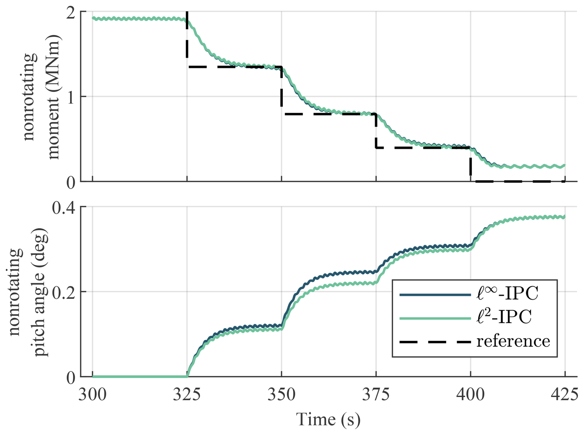
Figure 12 Time domain results of the staircase reference load in the nonrotating frame. Both control methods accurately follow the reference. The ℓ² IPC controller requires a smaller nonrotating pitch magnitude, indicating that it is more efficient.

Figure 13 shows the tilt contribution on the y axis and the yaw contribution on the x axis. So the response over time becomes a line on the tilt–yaw plane. Both controllers start with a reference above the open-loop load, resulting in no IPC action, which is thus equal to no IPC. Once the reference is reduced in its first step, the ℓ^∞ IPC controller only drives the moment vector down in the tilt direction since the load is naturally already below the yaw reference. This happens again in the second step of the reference load. Only when the tilt and yaw moments are equal and both constrained by the reference, at a phase of 45°, does the controller start actuating in yaw. The ℓ² IPC controller, on the other hand, drives the load directly to the origin and keeps the same phase of the pitch action. The ℓ² IPC method is thus more efficient since it does not spend control effort to change the phase of the load in the tilt–yaw plane. So the ℓ² IPC method requires a smaller pitch magnitude to track the same reference as ℓ^∞ IPC. With a reference of zero, both controllers are equal in operation to full IPC.

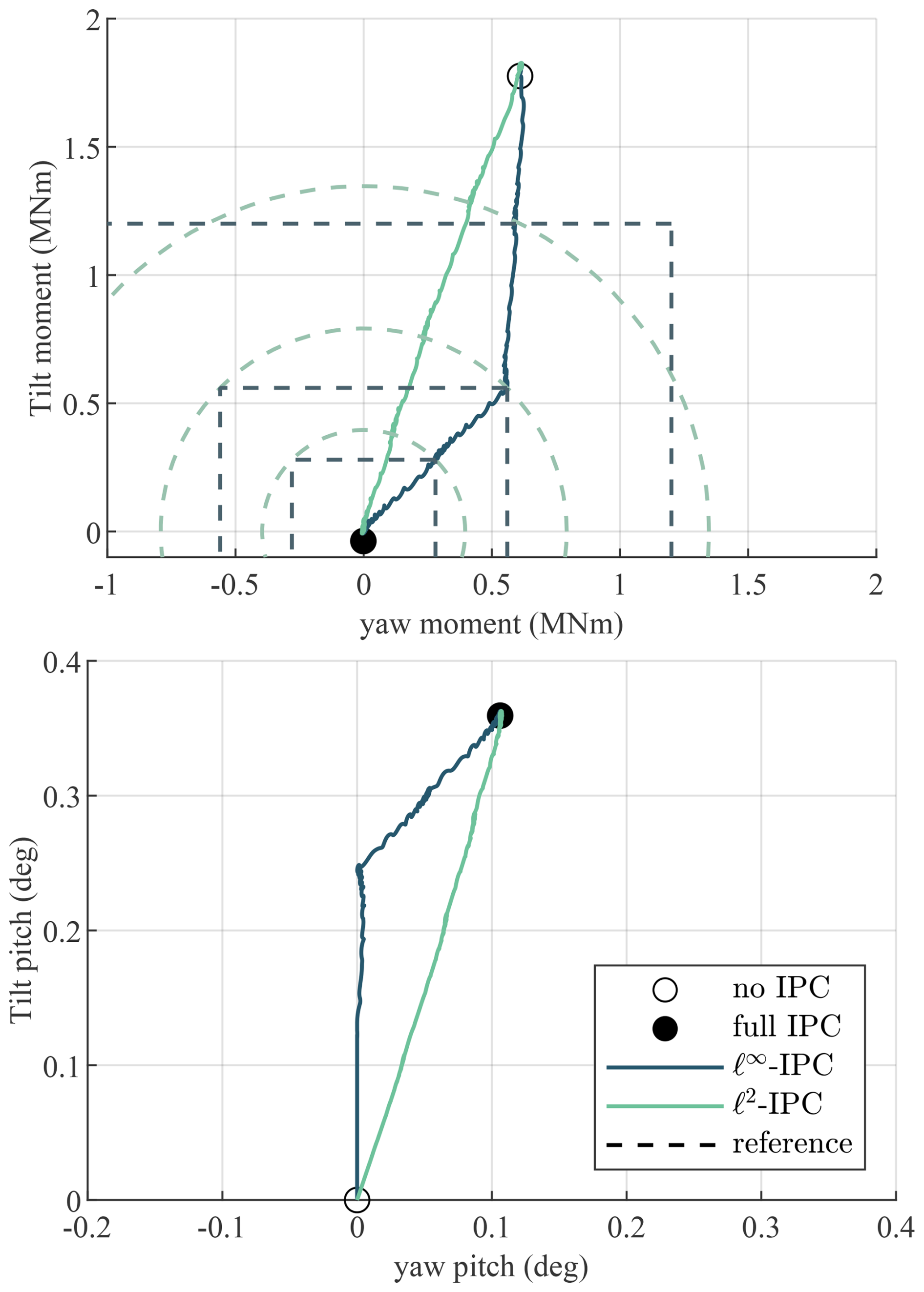
Figure 13 Time domain results plotted on the tilt–yaw plane for the staircase input. Both controllers start at no IPC and gradually go to full IPC in a few steps, resulting in a line in the tilt–yaw plane. The ℓ^∞ IPC method initially only drives the tilt moment to the tilt reference and only starts actuating in yaw when the yaw moment is constrained by the yaw reference. On the other hand, the ℓ² IPC method drives the load directly to the origin and keeps the same phase of the pitch action. By only spending control action on load reduction and not on a phase change of the load, ℓ² IPC is more efficient.

Furthermore, a pure shear input does not lead to a pure tilt moment response. Even though the wind is the strongest at the top of the tilt axis, the blade's dynamics cause the highest load to be experienced at the point indicated by no IPC. Each reference thus leads to a separate steady-state point, which is used to analyze the trade-off between actuator effort and load reduction.

5.3 The trade-off in laminar conditions

The previous section showed that ℓ² IPC achieves the same load reduction with a smaller pitch magnitude compared to ℓ^∞ IPC for a certain reference. This section expands on this by analyzing this trade-off for all operating points between no IPC and full IPC. For both control methods, 19 reference loads were analyzed, ranging from 0 N m (full IPC) to 2000 N m (above the open-loop load, so no IPC). The load reduction is measured using the damage equivalent load (DEL; see Eq. 9), while the actuator effort is measured using the actuator duty cycle (ADC; see Eq. 10).

Again, the first 300 s from the simulation is discarded, and the last 100 s of each reference load is used to calculate the actuator duty cycle and damage equivalent load. Since the system operates in steady state in laminar conditions, the DEL and ADC calculations do not require more data.

Figure 14 shows the trade-off between DEL and ADC for laminar conditions. For a reference load above the open-loop load, both control methods are equal in operation to no IPC. When the reference load is reduced, initially both control methods roughly achieve the same reduction in DEL for an increase in ADC. However, as the reference load is further reduced, the ℓ² IPC method reduces the DEL up to 8.4 % more than ℓ^∞ IPC using the same control effort. This is because the ℓ² IPC controller actuates in the same phase as the load, while the ℓ^∞ IPC controller also changes the phase of the load, as previously shown in Fig. 13, thus spending unnecessary control effort. As the reference load reaches zero, both controllers converge to full IPC. As the reference goes down further, the slope of the trade-off between DEL and ADC reduces in steepness as both controllers converge to full IPC. So close to full IPC, the reduction in DEL for a given increase in ADC is small. Both controllers perform identically to full IPC when their reference load is set to zero.

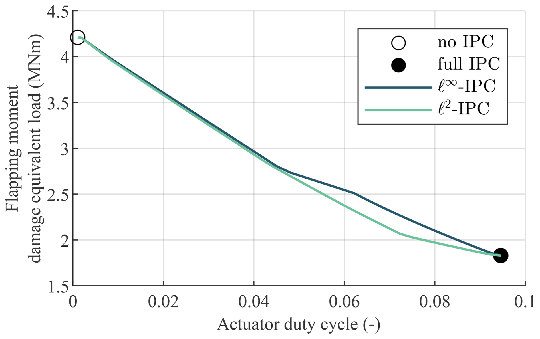
Figure 14 The trade-off when operating between no IPC and full IPC in laminar conditions. Close to full IPC in particular, ℓ² IPC achieves a larger reduction in the damage equivalent load of the flapping moment for the same actuator duty cycle compared to ℓ^∞ IPC.

Both proposed output-constrained IPC controllers can operate on any point between no and full IPC. In contrast, conventional IPC cannot trade off fatigue load and actuator effort in laminar conditions since the controller tuning does not affect the steady state, as discussed in Sect. 3.3.

Note that this result depends on the shear coefficient and wind speed, and the difference between the two controllers can be larger or smaller depending on these parameters. For example, if the open-loop load is a pure tilt moment, both controllers will have identical performance since the ℓ² norm and ℓ^∞ norm are equal for a pure tilt moment. The following section evaluates the performance of the open-loop load estimator when the wind shear coefficients vary.

5.4 Varying the wind shear coefficients

The previous results were obtained for a constant vertical wind shear coefficient of 0.07. This section shows that both control methods work for time-varying horizontal and vertical shear coefficients, which could arise from a changing boundary layer or wake impingement from upstream wind turbines when operating in a wind park.

When the shear coefficients of the wind change, the ℓ^∞ IPC method has to adjust the sign of the reference load and integrator saturation using the open-loop load estimation, while the ℓ² IPC method has to adjust the phase of the pitch signal based on this estimate.

An artificial wind field was generated, starting with an initial vertical shear coefficient of 0.07 and a horizontal shear coefficient of 0. In two steps, the vertical shear coefficient decreases to 0, while the horizontal shear coefficient goes to −0.07. This is done in laminar wind conditions to analyze the working mechanisms of the open-loop load estimator and its use by the two control methods. During the entire simulation, both control methods follow a constant reference of 1 MN m.

Figure 15 shows the results for the ℓ^∞ IPC method. Only the tilt signals are shown, but the same analysis applies to the yaw signals. At 300 s, the ℓ^∞ IPC controller follows the reference of 1 MN m accurately using a positive pitch angle. Furthermore, the original tilt moment is accurately estimated since it is equal to the no-IPC case, which does not do any individual pitch control, and its tilt moment is thus equal to the original tilt moment. The first wind shear change occurs at 340 s, and the tilt moment naturally decreases below the reference. To amplify the tilt moment to the reference, the controller would require a negative tilt pitch action. However, since the original tilt moment is correctly estimated to be positive, the pitch action is saturated on [0,∞) so that the controller does not amplify the load towards 1 MN m. Since the tilt moment is naturally below the reference, the controller sets its tilt pitch signal to zero, furthermore highlighting the advantage of output-constrained IPC. After the second wind shear change, at 380 s, the original tilt moment is correctly estimated to be negative, so the pitch action is saturated on $(-\mathrm{\infty },\mathrm{0}]$. Simultaneously, the reference sign is flipped, so the controller now drives the tilt moment to −1 MN m from an original tilt moment of about −1.4 MN m. This shows that in changing wind shear conditions, the ℓ^∞ IPC method correctly sets its pitch saturation and reference sign by estimating the sign of the open-loop load.

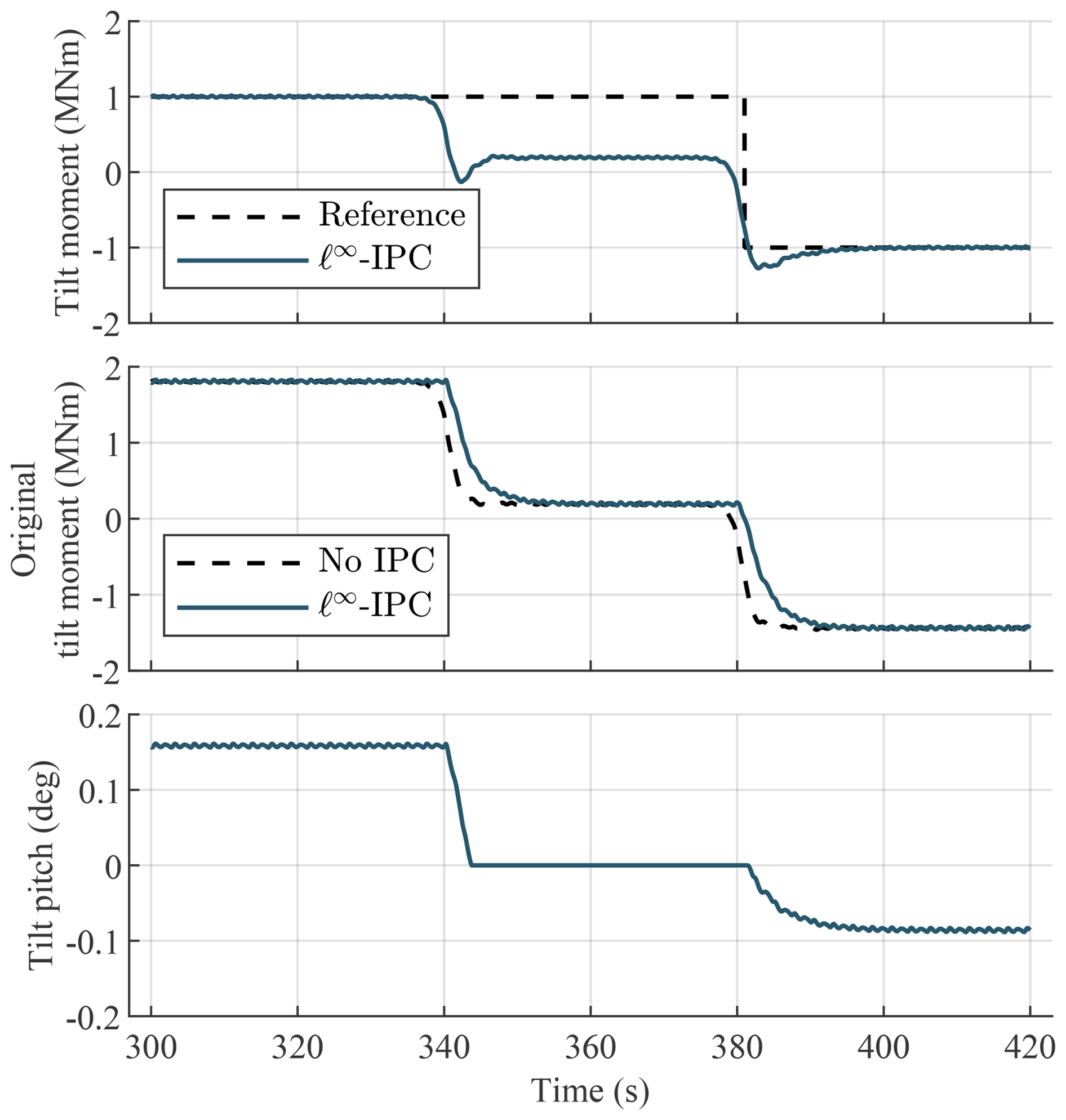
Figure 15 The ℓ^∞ IPC method first follows a reference of 1 MN m accurately. At the first wind shear change, the load naturally goes below this reference, and due to tilt pitch saturation, the controller does not amplify the load. Once its estimate of the open-loop load becomes negative, just after the second wind shear change, the reference sign and the controller saturation change, allowing the controller to reduce the tilt moment to −1 MN m.

Figure 16 shows the results for the same wind conditions but for the ℓ² IPC method. Note that the results are shown in magnitude and phase rather than along the tilt axis. At 300 s, the ℓ² IPC controller follows the reference of 1 MN m accurately using a pitch magnitude just below 0.2°. The phase of the original tilt is correctly estimated so that the phase of the pitch signal is ideal and matches that of a full-IPC controller. At the first wind shear change, at 340 s, the load again drops to below the reference and the pitch magnitude goes to zero. Even though the pitch magnitude is undefined, the pitch phase still follows the ideal phase since the ℓ² IPC method sets the phase of the pitch signal equal to the phase of the open-loop load, which is correctly estimated here. At the second wind shear change, at 380 s, the load is again constrained to 1 MN m after an initial overshoot. Note that, unlike in Fig. 15, the absolute value of the moment is shown and used by the controller, so the reference is not adjusted to be negative. Instead, the phase is adjusted. Note also that the final value of the pitch magnitude, which is just above 0.1°, is higher than in Fig. 15 because the previous figure only showed the tilt pitch signal. This is done because the ℓ^∞ IPC method uses a decoupled tilt and yaw controller, whereas the ℓ² IPC method acts on the magnitude by using the phase of the signals, so different signals are relevant when showing the results of this test case. The next section analyzes the controller performance in continually varying conditions using turbulent wind.

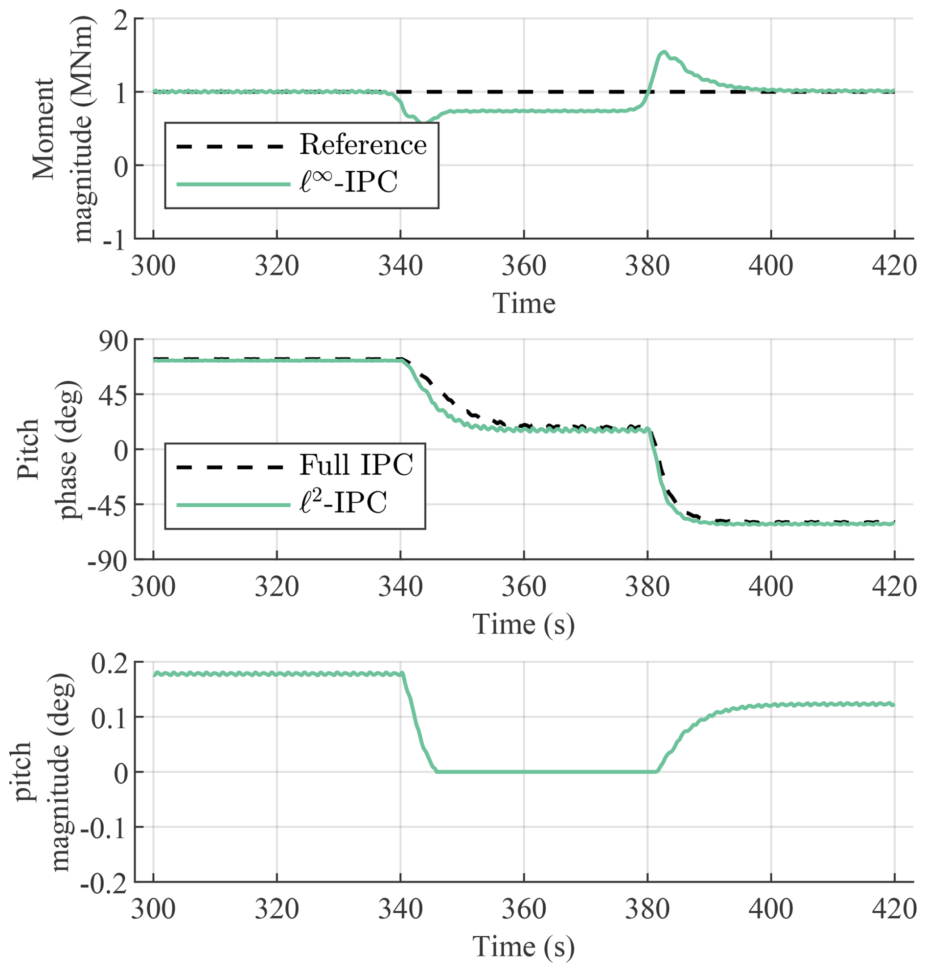
Figure 16 By estimating the phase of the open-loop load, the ℓ² IPC method actuates in the ideal phase. The ideal phase is equal to the phase of the pitch signal of full IPC.

5.5 The trade-off in turbulent wind conditions

This section analyzes the effectiveness of the proposed output-constrained IPC methods in realistic turbulent wind conditions. To this end, the trade-off between DEL and ADC for laminar wind conditions, previously shown in Fig. 14, is extended to turbulent wind conditions and compared to the baseline, discussed in Sect. 3.3.

Similarly to the baseline, the turbulent wind fields are generated using TurbSim (Jonkman, 2009) with 8 % turbulence intensity for 10 different seeds, each with 30 min of useful data to obtain statistically significant results.

To analyze the different operating points between no IPC and full IPC, the ℓ^∞ IPC and ℓ² IPC methods were run using multiple reference loads between 10 MN m (always above the open-loop load, so no IPC) and 0 MN m (full IPC). Note that the no-IPC load is substantially higher than for the laminar conditions due to load peaks as a result of turbulence.

Additionally, the data from the full-IPC controller with a gain crossover frequency of 0.2 rad s⁻¹, as previously shown in Fig. 5, are used to compare to the proposed control methods.

Figure 17 shows the trade-off between DEL and ADC in turbulent wind conditions and compares the ℓ^∞ IPC and ℓ² IPC methods to the baseline. Since each operating condition is run for 10 different turbulent wind seeds, there is a distribution of results. This distribution is assumed to be Gaussian, and the mean is shown as a line connecting the data points from each operating condition. The shaded region around this line represents 1 standard deviation from the mean. Since no and full IPCs have no parameters to tune, they only have a single mean and are thus shown as a data point with error bars representing the standard deviation.

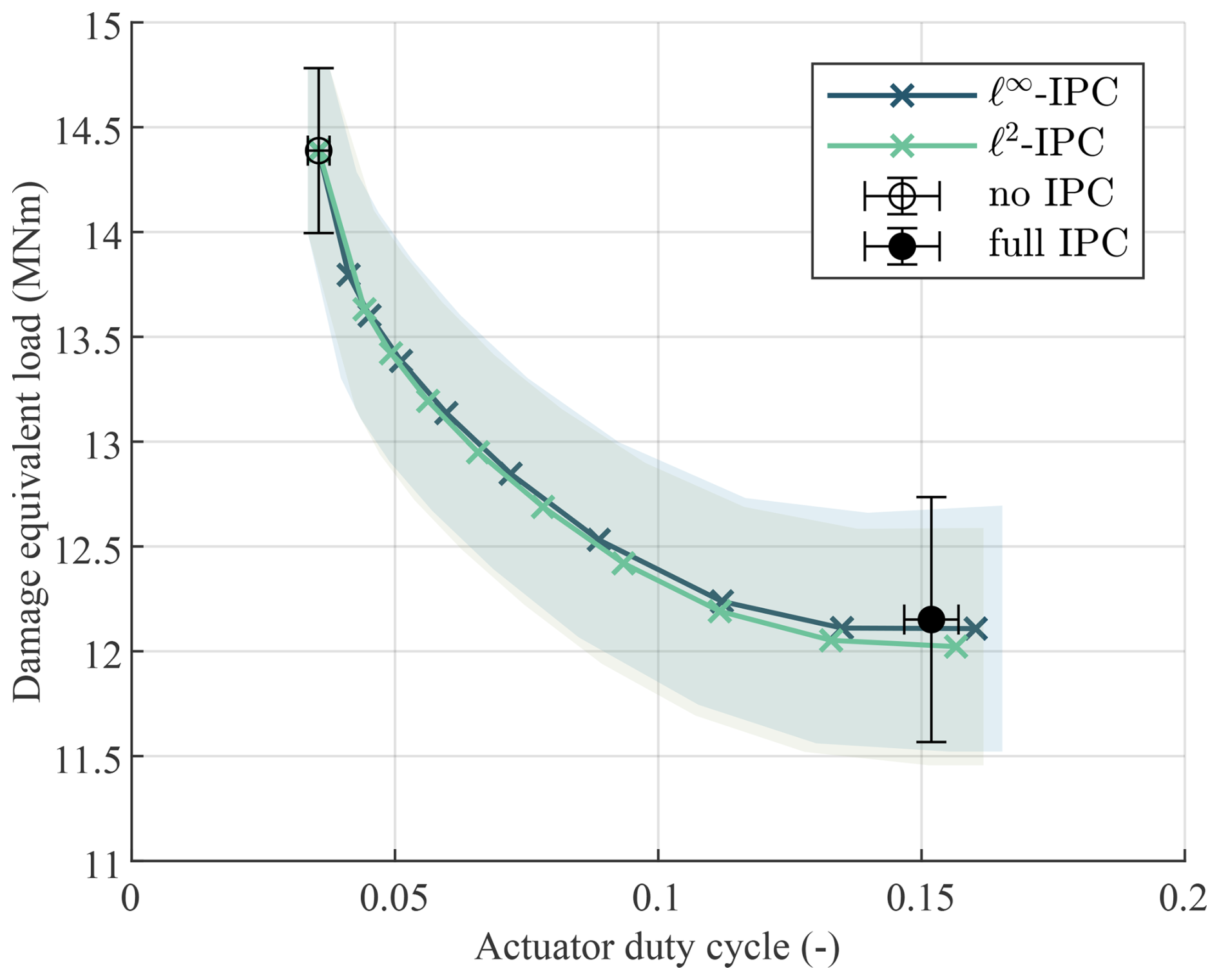
Figure 17 The trade-off between DEL and ADC when operating between no IPC and full IPC with 8.0 % turbulence. The ℓ^∞ IPC and ℓ² IPC methods use a change in reference load between 10 MN m (corresponding to no IPC) and 0 MN m (corresponding to full IPC). The error bars (for no and full IPC) and the shaded region (for ℓ^∞ IPC and ℓ² IPC) represent the standard deviation (1σ) from the mean. The output-constrained IPC methods have a nonlinear trade-off and achieve 87 % of the reduction in DEL at just 50 % of the increase in ADC compared to the full-IPC controller with the same crossover frequency (0.2 rad s⁻¹).

First, both ℓ^∞ IPC and ℓ² IPC smoothly transition between no IPC and full IPC by adjusting their reference loads. By setting the reference above the open-loop load, the controllers both converge to no IPC, while a reference of 0 MN m results in operation close to the full-IPC controller that uses the same crossover frequency, namely 0.2 rad s⁻¹. The trade-offs that ℓ^∞ IPC and ℓ² IPC achieve are highly curved and do not go in a straight line from no IPC to full IPC, as was the case for changing the gains of full IPC, previously shown in Fig. 5. At the operating point where ADC = 0.055, both methods achieve 50 % of the reduction in DEL with just 16.4 % of the increase in ADC compared to full IPC tuned with the same crossover frequency. Furthermore, at ADC = 0.094, both methods achieve 87 % of the reduction in DEL with just 50 % of the increase in ADC. Thus, a significant decrease in actuator effort is achieved by aiming for a slightly lower reduction in fatigue loads using output-constrained IPC. The relative changes in fatigue load and actuator duty cycle are easier to observe in a normalized plot, given in Appendix A.

This is caused by the nonlinearity of the DEL calculation. Closer to no IPC, the controllers only attenuate the largest load peaks, which proportionally contribute more to the DEL than smaller peaks, which are only attenuated closer to full IPC, leading to diminishing returns.

Second, the difference between the two control methods is minimal in turbulent conditions, though ℓ² IPC is slightly more efficient when operating closer to full IPC. However, this advantage is well within 1 standard deviation. In laminar conditions, ℓ² IPC was clearly more efficient because it did not change the phase of the load. The difference in phase between ℓ^∞ IPC and ℓ² IPC is the highest when the open-loop load is 22.5°+k45°, where k∈ℕ. But when the phase is 0°+k45°, ℓ^∞ IPC does not change the phase, and the two methods have an equal performance. In turbulent wind conditions, the phase of the open-loop load is constantly changing, so the large advantage of ℓ² IPC is not as pronounced anymore.

The ℓ^∞ IPC and ℓ² IPC methods were only run with a crossover frequency of 0.2 rad s⁻¹, while the full-IPC controller was run for a grid search over multiple crossover frequencies, as discussed in Sect. 3.3. When lowering the gain of the full-IPC controller, it moves towards no IPC in a more straight line, not taking advantage of the nonlinearity of the DEL. Its lower gain ensures that it achieves a smaller load reduction, but the phase of the control action also starts to lag behind the optimal phase, thus reducing efficiency. The proposed output-constrained control methods do not suffer from this effect since their load reduction and bandwidth are separated into the reference load set point and controller tuning. Furthermore, the full-IPC controller cannot reach the no-IPC operating point by lowering the crossover frequency further because lowering its gain becomes unpractical because the time constant of such a controller would be larger than 100 s, as discussed in Sect. 3.2.

Lastly, in a few simulations, it was observed that the maximum pitch rate of 2° s⁻¹ was exceeded. This occurred in two scenarios: first, for both controllers when using a reference load of 500 or 0 kN m and thus requiring a large pitching action. Second, some small step changes in pitch angle were observed for the ℓ^∞ IPC controller, which happened when the saturation of the controller switched, so when the sign of the estimated open-loop load changed. In the latter case, actuator dynamics, which were neglected in this work, would smooth these step changes, while in the first case, a slower tuning, or combining output-constrained IPC with input-constrained IPC, could avoid exceeding the maximum pitch rate.

6 Conclusions

In this work, we have explored the entire operating region between no and full IPC, using two newly proposed output-constrained IPC methods, enabling the trade-off between actuator effort and load reduction, achieving an 87 % reduction with just 50 % of the actuation effort. The two methods, ℓ^∞ IPC and ℓ² IPC, are natural extensions of the conventional IPC implementation based on the multiblade coordinate transformation, thus contributing to industry adoption.

In laminar conditions, both control methods accurately follow any load reference and thus operate on any point between full IPC and no IPC. In these conditions, ℓ² IPC is more efficient since it does not use actuator effort to change the phase of the load. The open-loop load estimator, used by the ℓ^∞ IPC method to set its reference sign and integrator saturation and used by the ℓ² IPC method to set the phase of the control action, accurately reconstructs the open-loop load using a steady-state estimate.

In turbulent wind conditions, both controllers can operate on any point between no IPC and full IPC. The trade-off is highly curved, and both control methods achieve 87 % of the load reduction, measured in damage equivalent load (DEL), with just 50 % of the actuator effort, measured in actuator duty cycle (ADC), compared to full IPC with the same controller tuning. This is the most important result of this work, and it shows that these controllers not only facilitate the trade-off between no and full IPC, but also achieve an excellent trade-off between DEL and ADC. Since high ADC is a barrier to the industrial application of IPC, these methods allow the industry to gain most of the benefits with little downsides.

In this work, both control methods are tuned with a crossover frequency of 0.2 rad s⁻¹, while in turbulent conditions, full IPC achieves the highest load reduction with a crossover frequency of 0.75 rad s⁻¹. Future work will optimally tune the proposed control methods to find the Pareto front between DEL and ADC by varying the reference load, crossover frequency, and open-loop load estimation frequency, and will quantitatively compare the performance to input-constrained IPC methods or a combined input- and output-constrained IPC method. The optimal tuning would highly depend on the wind speed, and an optimization over all nominal operating conditions could show at which wind speeds the trade-off between DEL and ADC is most favorable. Furthermore, instead of using a fixed reference load for each wind speed, the reference load could be defined as a certain percentage of the estimated open-loop load, adding a feedback loop and making the controller adaptive to changing inflow conditions.

Since these control methods make a smooth trade-off between no and full IPC, they will also be integrated into a wind turbine control co-design framework. The large reduction in fatigue loads, with a small effect on actuator fatigue, might lower the material costs of the blades with a small increase in the cost of the pitch actuation system, thus lowering the overall cost of wind turbines.

Appendix A: The normalized trade-off in turbulent wind conditions

To normalize the results of Fig. 17, no IPC is taken as the baseline, and the relative performance with respect to full IPC is calculated. Therefore, a 0 % ADC increase and 0 % DEL decrease correspond to no IPC, and a 100 % ADC increase and 100 % DEL decrease correspond to full IPC. The relative change in ADC is calculated using

$$\begin{array}{}\text{(A1)}& \text{ADC increase \%}={\displaystyle \frac{\text{ADC}-{\text{ADC}}_{\text{no-IPC}}}{{\text{ADC}}_{\text{full-IPC}}-{\text{ADC}}_{\text{no-IPC}}}},\end{array}$$

and the relative decrease in DEL is calculated in a similar way. Figure A1 shows this normalized trade-off, where it is easier to see that both methods achieve an 87 % reduction in DEL at just a 50 % increase in actuator effort with respect to no IPC.

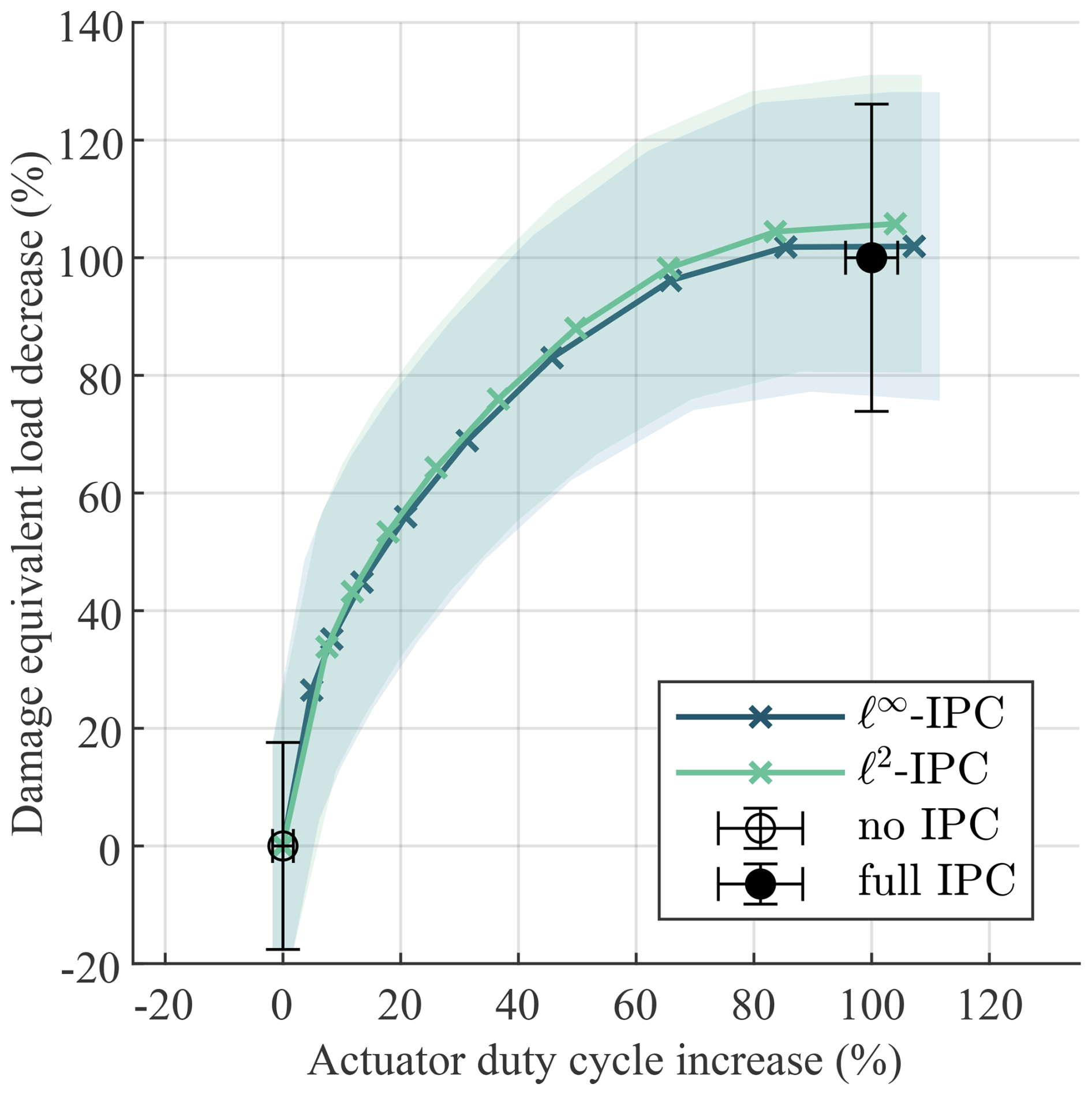
Figure A1 The normalized trade-off when operating between no IPC and full IPC with 8.0 % turbulence. The trade-off is normalized so that no IPC has a 0 % load reduction at a 0 % actuator effort increase, while full IPC with a crossover frequency of 0.2 rad s⁻¹ achieves a 100 % load reduction at a 100 % actuator effort increase. The two output-constrained methods achieve a relatively high amount of load reduction with a small actuator effort increase compared to changing the crossover frequency of full IPC.