Data assimilation of generic boundary layer flows for wind turbine applications – an LES study

Providing date- and site-specific turbulent inflow fields for large-eddy simulations (LESs) of the flow through wind turbines becomes increasingly important for reliable estimates of power production. In this study, data assimilation techniques are applied to adapt the atmospheric inflow field towards previously defined wind profiles. A standard and a modified version of the Newtonian relaxation technique and an assimilation method based on the vibration equation are implemented in the geophysical flow solver EULAG. The extent to which they are able to adapt mean horizontal wind velocities towards target profiles and the impact on atmospheric turbulence of an idealized LES are investigated. The sensitivity of the methods to grid refinement is analyzed. The method based on the vibration equation is suited for fine grids (dx = dy = dz = 5 m), which is a common grid resolution for wind energy studies. Furthermore, the vibration method is used to nudge the zonal and meridional inflow velocities of an idealized atmospheric simulation towards velocity profiles representing a weakly stably stratified atmospheric boundary layer (ABL) at the wind farm site WiValdi at Krummendeich, Germany. On-site wind measurements and the output of mesoscale simulations are evaluated to define the target velocity profile. The assimilation method based on the vibration equation is able to adapt the zonal and meridional velocity components of an atmospheric flow, while negative effects on the atmospheric turbulence could be reduced. In a final step, the assimilated flow field is taken as inflow for a wind turbine simulation, which then shows the characteristic structures of a wake in the ABL. This study shows the suitability of the vibration method for adapting inflow fields for wind energy purposes and presents the advantages and disadvantages of the method.

1 Introduction

The growing demand for wind energy is accompanied by a wide range of challenges as structural components and technical characteristics of wind turbines are getting more and more sophisticated. In particular, the mutual interaction of wind turbine wakes in wind farms and their response to the transient atmospheric flow field are grand challenges in wind energy research (cf. Veers et al., 2023). General attention is paid to the performance of the turbines and the loads on the blades, which are mainly determined by turbulence in the atmospheric boundary layer (ABL) (cf. Hansen, 2013; Wharton and Lundquist, 2012). The general question is how to maximize the harvested power of a wind turbine at a certain location under specific operational conditions. One of the decisive factors in answering this question is the atmospheric situation under which the wind turbines are operating. Knowledge of the thermal stratification and the flow conditions is becoming increasingly important because rotor diameters are getting larger and the hub heights are getting higher, thus covering a greater depth of the ABL. Better knowledge of the impact of different atmospheric characteristics like the vertical gradient of the horizontal velocity and turbulence intensities impacting a wind turbine and its wake is therefore essential.

The recent opening of the wind energy research farm WiValdi (https://windenergy-researchfarm.com, last access: 8 August 2025; Wind Validation) in Krummendeich, northern Germany, on 15 August 2023 by the German Aerospace Center (DLR) and the Research Alliance Wind Energy (FVWE, Forschungsverbund Windenergie, https://www.fvwe.uni-oldenburg.de, last access: 8 August 2025) offers a timely opportunity to expand our knowledge on this topic. The wind park consists of two Enercon E-115 EP3 turbines with hub heights of 92 m and rotor diameters of D = 116 m separated by a rather narrow spacing of 4.4 D. In addition, a smaller custom-built turbine is currently under construction. The flow fields and the turbine wakes at the wind park can be measured in great detail by the vast observational network located on-site. This network includes a series of measuring masts, multiple Doppler wind lidar (DWL) instruments, and a microwave radiometer.

Even with a really dense observational network and a large number of field measurements that can provide quasi-reliable 3D pictures of the atmospheric situation, there are still natural spatial and temporal limitations in resolving all motion modes affecting the response of wind turbines to the atmospheric flow. In order to close such scale gaps, numerical simulations can provide 3D flow fields of the entire wind park with very high spatial and temporal resolutions. In particular, large-eddy simulation (LES) models have been proven to be a useful and powerful tool to compute these turbulent flow fields. In contrast to simulations based on Reynolds-averaged Navier–Stokes (RANS) equations, LESs are capable of resolving turbulence in the flow. In addition, LESs are computationally less expensive than direct numerical simulations (DNSs) because the subgrid-scale (SGS) contribution to the turbulence is parameterized.

LESs are also frequently used to evaluate the effects of thermal stratification of the ABL on the wakes of wind turbines and wind farms for various atmospheric conditions (cf. Bhaganagar and Debnath, 2014; Abkar et al., 2016; Vollmer et al., 2016; Englberger and Dörnbrack, 2018). Particular emphasis has been placed on a distinctive thermal ABL stratification (neutral, convective, stable) on the flow around a single wind turbine and the flow in a wind farm (Porté-Agel et al., 2020). However, the majority of these studies conduct their basic research with idealized LESs that are characterized by no large-scale and mesoscale forcing and by no temporal or spatial variation of the associated pressure gradient. The representation of real, measured flow conditions like those observed in WiValdi, however, cannot be addressed reliably with such purely idealized setups.

One way to generate site-specific atmospheric flow conditions is to couple mesoscale simulations (e.g., simulations of the Weather Research and Forecasting Model (WRF); Skamarock et al., 2019) with LESs (e.g., Aitken et al., 2014; Sanchez Gomez and Lundquist, 2020; Kilroy et al., 2024). Recent advances in this research field has been made by the Mesoscale to Microscale Coupling project sponsored by the US Department of Energy (cf. Haupt et al., 2023). There, the authors emphasize the complexity of modeling the correct energy transfer from the largest scales of motion to the scales within the ABL from which the wind turbines generate electrical energy. Further, they note that simulations from the mesoscale down to the microscale (for example, with the mentioned WRF–LES coupling) are exceptionally computationally expensive. Therefore, such elaborate methods cannot be used to simulate a variety of different atmospheric situations, assuming that both the computing time and the physical time required to perform the simulations are far too long. Other approaches including a technique that combines atmospheric modeling and machine learning try to generate time-resolved wind inflow data for turbines (cf. Rybchuk et al., 2025).

An alternative approach to circumvent the expensive mesoscale and microscale coupling is to conduct idealized numerical simulations coupled with a suitable data assimilation method for providing date- and site-specific turbulent flow conditions. This numerical approach is computationally less expensive. In such a setup, data assimilation methods are assumed to transfer the given mesoscale information (wind and stability profiles) onto the microscale (cf. Stauffer and Seaman, 1990; Neggers et al., 2012; Maronga et al., 2015; Nakayama and Takemi, 2020; Allaerts et al., 2020).

In general, those methods apply a damped harmonic oscillator as an additional forcing in the governing equations of motion. Commonly, this forcing term can consist of a damping (proportional) and an oscillating (integral) part (e.g., Spille-Kohoff and Kaltenbach, 2001). In the case of Newtonian relaxation, only the damping part is considered. Here, the numerically calculated profiles of wind, temperature, and humidity are adjusted to given target profiles (which can either come from measurements or be extracted from the output of mesoscale model simulations) using a specific relaxation timescale, which is a free parameter of this method.

The relaxation timescale should be long enough (∼ hours) that the small-scale turbulence in the LES is not affected by it; however, it needs to be small enough to be able to adapt the LES towards mesoscale characteristics in a reasonable time (Neggers et al., 2012). An issue, however, is that turbulence intensity is often overly reduced using Newtonian relaxation. The investigations by Allaerts et al. (2020, 2023) present an “indirect profile assimilation” method. It is described as an internal forcing technique deduced from mesoscale variables (wind speed and temperature), including the time and height history of these variable in the LES. Their grid assimilation method acts in the numerical simulation at every grid point in the domain and achieves an equilibrium state with the desired atmospheric mean characteristics and turbulent statistics. They tested the approach with the damping part and a combination of both damping and oscillating, with quite similar results. Further, Stipa et al. (2024) developed another domain relaxation approach by applying the proportional and integral part, which is additionally able to prevent inertial oscillations, making it well-suited for wind park approaches.

Another data assimilation technique described in Nakayama and Takemi (2020) is based on the oscillating part only, which has the property of fluctuating around the target mean values. This integral forcing is controlled by the natural frequency of the flow field, which has to be set appropriately in order not to damp turbulent fluctuations. We refer to this method in the following as the vibration method. Their approach includes a precursor simulation driven by a pressure gradient. This precursor is used as inflow for a following simulation where the assimilation technique is applied only in a nudging area which is smaller than the simulation domain. Nakayama and Takemi (2020) emphasized the advantage of this method in handling the turbulence intensity in comparison to the Newtonian damping.

While the methods of Allaerts et al. (2020) and Stipa et al. (2024) have been directly developed for wind turbine applications, the method of Nakayama and Takemi (2020) has been applied only at a rather coarse resolution of 40 m horizontally and relaxes only the horizontal wind field. However, the application of this method to higher-resolved LESs including wind turbines would have the advantage that it can reproduce an assimilation of simultaneous measurements, is not limited to horizontal homogeneity, and could possibly be applied in complex terrain. Therefore, it also seems well-suited for wind energy applications. Considering the DLR wind farm WiValdi, it seems to be a worthwhile endeavor to modify the method of Nakayama and Takemi (2020) so that it can be applied in this first approach to a single wind turbine to assimilate more realistic observed wind profiles, with the aim of calculating more complex inflow cases that do not lose their turbulent atmospheric characteristics.

An LES of a wind turbine or a wind farm, which is conducted with open lateral boundary conditions, requires, in addition to the input of the mesoscale information as horizontal mean values of the corresponding profiles, a turbulent inflow field, which synchronously feeds turbulence in the inflow region. There are different numerical approaches for generating the required turbulent inflow fields, especially for wind turbine simulations (e.g., Bhaganagar and Debnath, 2014; Abkar et al., 2016; Englberger and Dörnbrack, 2017). One possibility is the generation of synthetic turbulence fields, as proposed by Mann (1994). These stochastic models avoid high computational costs but they are not physical models in the sense that they satisfy the conservation laws (cf. Naughton et al., 2011). Turbulent atmospheric inflow fields which are more close to observations are generated by LESs. Therefore, another possibility is the production of a limited number of idealized precursor simulations, representing specific atmospheric conditions (neutral, convective, stable). These atmospheric precursor simulations are computationally expensive because turbulence has to spin up in the domain of interest until key flow parameters (vertical gradient of horizontal velocity, turbulence kinetic energy – TKE) match anticipated characteristics in the ABL. Therefore, one main positive effect of the method of Nakayama and Takemi (2020) could be the application of one precursor simulation to a variety of measurements (occurring under relatively similar atmospheric conditions, for example stratification and/or geostrophic winds). In order to account for the broad range of possible atmospheric situations, multiple precursor simulations are required. The proposed method here is only meaningful if the measured key values of wind speed and TKE (and also lapse rate in the case of stratified situations) are approximated by the precursor simulation.

The main goal of this work is the application and assessment of the vibration method in wind energy research. Since the method can use the measured horizontal wind as a background profile, it offers a cost-effective way to simulate the effects of specific atmospheric properties on the wake of wind turbines with high spatial resolution. In general, data assimilation techniques applied in wind energy research pose a lot of open questions (Allaerts et al., 2020, 2023; Stipa et al., 2024). With this study, we want to make a first step towards the generation of site-specific inflow fields for wind turbines using data assimilation where the additional forcing due to the assimilation is applied in a dedicated region of the computational domain upstream of the wind turbine.

The outline of this paper is as follows. The numerical model EULAG, the Newtonian relaxation methods, the vibration assimilation method, the measurements, and the numerical setup are presented in Sect. 2. In Sect. 3, we perform idealized LESs to reproduce the results of the coarse-resolution method of Nakayama and Takemi (2020). Section 4 adapts this vibration method towards a wind-energy-relevant fine resolution for their neutral boundary layer (NBL) case. Here, we test the applicability of the vibration method at fine resolution and compare it to the performance of both Newtonian approaches. A special focus is on the impact of the discussed assimilation methods with regard to the characteristic atmospheric turbulence. As our final aim is to simulate real atmospheric situations, which, for example, may include veering inflows, Sect. 5 exemplifies how the idealized approach can be modified towards the reproduction of a measured near-stable atmospheric situation in the wind farm WiValdi. Here, we focus on the parameter space of the vibration approach and the importance of a proper precursor simulation and use a combination of measurements and a WRF simulation for creating target wind profiles. Finally, we test the applicability of the vibration method in a wind turbine simulation in Sect. 6 where the wind turbine is exposed to the generated inflow from Sect. 5. This is a first test case of the developed tool chain using a precursor simulation and the vibration method to generate a stably stratified atmospheric inflow situation for a wind turbine and the subsequent simulation of the wake behind the wind turbine. Conclusions are then drawn in Sect. 7.

2 Methodology

2.1 The numerical model EULAG

The dry and incompressible flow inside the ABL is simulated with the geophysical flow solver EULAG (Prusa et al., 2008). EULAG is an established computational model which has been used for a wide range of physical scenarios: the simulation of urban flows (Smolarkiewicz et al., 2007), internal gravity waves (Mixa et al., 2021; Dörnbrack, 2024), turbulent atmospheric flows (Margolin et al., 1999), and even solar convection (e.g., Elliott and Smolarkiewicz, 2002). The name EULAG refers to the two possible ways to solve the equations of motion: either in Eulerian, i.e., flux form (Smolarkiewicz and Margolin, 1993), or in semi-Lagrangian, i.e., advective form (Smolarkiewicz and Pudykiewicz, 1992). The advective terms in the fluid equations are approximated by the iterative finite-difference algorithm MPDATA (multidimensional positive-definite advection transport algorithm), which is second-order accurate, positive-definite, conservative, and computationally efficient (Smolarkiewicz and Margolin, 1998). A detailed explanation of EULAG can be found in Smolarkiewicz and Margolin (1998) and Prusa et al. (2008).

For the simulations in this study, the following set of non-hydrostatic Boussinesq equations with constant density ρ₀=1.1 kg m⁻³ are solved for the Cartesian velocity components $\mathit{v}=(u,v,w)$ and for the potential temperature perturbation ${\mathrm{\Theta }}^{\prime }=\mathrm{\Theta }-{\mathrm{\Theta }}_{\mathrm{e}}$; see Smolarkiewicz et al. (2007) in general and Englberger and Dörnbrack (2018) for wind turbine applications:

$$\begin{array}{}\text{(1)}& {\displaystyle }\mathbf{\nabla }\cdot \mathit{v}=\mathrm{0},\text{(2)}& {\displaystyle }\begin{array}{rl}{\displaystyle \frac{\mathrm{d}\mathit{v}}{\mathrm{d}t}}& =\underset{\text{pressure gradient}}{\underbrace{-\mathbf{\nabla }\left({\displaystyle \frac{p^{\prime }}{{\mathit{\rho }}_{\mathrm{0}}}}\right)}}+\underset{\text{buoyancy}}{\underbrace{\mathit{g}{\displaystyle \frac{{\mathrm{\Theta }}^{\prime }}{{\mathrm{\Theta }}_{\mathrm{0}}}}}}-\underset{\text{Coriolis force}{\mathit{F}}_{\mathrm{cor}}}{\underbrace{\mathrm{2}\mathbf{\Omega }\times (\mathit{v}-{\mathit{v}}_{\mathrm{e}})}}\\ & +\underset{{\mathit{F}}_{\mathrm{WT}}}{\underbrace{{\displaystyle \frac{\mathit{F}}{{\mathit{\rho }}_{\mathrm{0}}}}}}-\mathit{f}+\mathit{V}+\underset{{\mathit{F}}_{\mathrm{abs}}}{\underbrace{\mathit{\alpha }(\mathit{v}-{\mathit{v}}_{\mathrm{e}})}},\end{array}\text{(3)}& {\displaystyle \frac{\mathrm{d}{\mathrm{\Theta }}^{\prime }}{\mathrm{d}t}}=-\mathit{v}\mathbf{\nabla }{\mathrm{\Theta }}_{\mathrm{e}}+\mathit{H}+\mathit{\beta }{\mathrm{\Theta }}^{\prime }.\end{array}$$

In these equations Θ₀ denotes the constant reference value of the potential temperature and Θ_e is its balanced ambient/environment state. The operators $\frac{\mathrm{d}}{\mathrm{d}t}$, ∇ and ∇⋅ represent the total derivative, the gradient, and the divergence. p^′ symbolizes the pressure perturbations, $\mathit{g}=(\mathrm{0},\mathrm{0},-g)$ is the acceleration due to gravity, and F_cor indicates the Coriolis force with the angular velocity vector of the Earth $\mathbf{\Omega }=(\mathrm{0},\mathrm{0},\mathrm{\Omega }\sin (\mathit{\varphi }\left)\right)$, where ϕ is the latitude. The Coriolis parameter is $f=\mathrm{2}{\mathrm{\Omega }}_z=\mathrm{1.0}\times {\mathrm{10}}^{-\mathrm{4}}$ s⁻¹ for midlatitudes and v_e is the background or environmental velocity.

The SGS terms V and H indicate turbulent dissipation of momentum and diffusion of heat, respectively. The simulations within this study are all conducted with a TKE closure (Margolin et al., 1999). F_abs is an absorber to attenuate the solution at the lateral and model top boundaries (cf. Smolarkiewicz et al., 2007). A similar absorber is used in Eq. (3). α and β indicate inverse timescales. f denotes the additional forcing due to the selected data assimilation techniques, which are presented in Sect. 2.2; see Eqs. (4), (6), and (7).

In the simulation with a wind turbine, F_WT corresponds to the forces generated by the rotor blades. The wind turbine is implemented with the blade-element momentum theory as a rotating actuator disk, (Mirocha et al., 2014). Unfortunately, the blade data for the Enercon E-115 EP3 turbine necessary for the calculation of the forces on the flow induced by the blades are currently not available. The Enercon E-115 EP3 turbines at the DLR wind park WiValdi have a hub height of h_hub=92 m and a rotor diameter D = 116 m. Therefore, the simulation is conducted with the blade data of the 5 MW reference wind turbine defined by the National Renewable Energy Laboratory (NREL) (Jonkman et al., 2009). This wind turbine was selected, as it has a similar hub height (h_hub=90 m) and rotor diameter (D = 126 m).

2.2 Assimilation methods

There are several factors limiting the accuracy and comparability of LESs with real case measurements and field observations. On the one hand, the truncation errors due to discretization limit the accuracy of the numerical model (e.g., Arcucci et al., 2017; Neggers et al., 2012). On the other hand, many small-scale meteorological processes due to mesoscale phenomena, e.g., frontal passages, atmospheric waves, or diurnal circulations like land–sea breezes, cannot be represented correctly by LESs (e.g., Allaerts et al., 2020). Concerning simulations with wind turbines, the grid spacing has to be small enough to account for forces generated at the blades. In a stable boundary layer (SBL), the turbulent scales are very small due to the thermal stratification and can only be partially resolved even with fine grid spacings ($\mathrm{d}x=\mathrm{d}y=\mathrm{d}z\le \mathrm{5}$ m). Therefore, the entire domain size of LESs is restricted to the order of kilometers and mesoscale phenomena cannot be represented within these simulations, as their scales range from 10 km to more than 100 km (Haupt et al., 2023).

In order to resolve this issue, data assimilation techniques of the simulated flow field towards observational data are widely used in numerical models in order to enhance the realism of LESs. Typically the additional forcing of the assimilation is applied in the whole simulation area (e.g., Maronga et al., 2015; Allaerts et al., 2020; Stipa et al., 2024). In this work we focus on an assimilation which is only applied in a dedicated region of the simulation domain which spans the whole height (z) and width (y) of the domain but includes only a part of the streamwise length (x) of the domain. For example, the grid-nudging method relies on the definition of a local Newtonian relaxation according to Eq. (6) of Nakayama and Takemi (2020):

$$\begin{array}{}\text{(4)}& {\mathit{f}}_N(x,y,z,t)=\mathrm{damp}\left(x\right){\mathit{\rho }}_{\mathrm{0}}{\displaystyle \frac{\mathit{v}(x,y,z,t)-{\mathit{v}}_{\mathrm{OBS}}(z,t)}{\mathit{\tau }}}\end{array}$$

with

$$\begin{array}{}\text{(5)}& \begin{array}{rl}& \mathrm{damp}\left(x\right)={\sin }^{\mathrm{2}}\left[{\displaystyle \frac{\mathit{\pi }}{\mathrm{2}}}\left(\mathrm{1}-{\displaystyle \frac{x_{\mathrm{nud}}-x}{x_l}}\right)\right],\\ & x_{\mathrm{nud}}-{\displaystyle \frac{x_l}{\mathrm{2}}}\le x\le x_{\mathrm{nud}}+{\displaystyle \frac{x_l}{\mathrm{2}}}.\end{array}\end{array}$$

In Eq. (4), f_N symbolizes the forcing term f in the momentum conservation (Eq. 2) for the local Newtonian relaxation, v is the instantaneous velocity vector at a certain grid point, and v_OBS is the vector of the target velocity values given through observational data. In this study, we consider only the relaxation of the zonal and meridional velocity components.

As the additional forcing due to the data assimilation is only applied in a nudging area a bell-shaped damping function damp(x) acts in the zonal direction to prevent numerical artifacts at the borders of the nudging area. x_nud is the center of nudging area and x_l the length of the damping layer in the zonal direction. The relaxation timescale τ has to be chosen to be small enough to generate a considerable forcing towards the target data but not too small such that small-scale atmospheric turbulence is suppressed (cf. Neggers et al., 2012; Maronga et al., 2015). The local Newtonian relaxation according to Eq. (4), which is introduced in Eq. (2), can provoke the damping of small-scale turbulent structures in the ABL, which is mentioned by Neggers et al. (2012), Maronga et al. (2015), Heinze et al. (2017), and Nakayama and Takemi (2020).

A modification of the local Newtonian relaxation of Eq. (4) is applied (e.g., Maronga et al., 2015; Heinze et al., 2017; Allaerts et al., 2020):

$$\begin{array}{}\text{(6)}& {\mathit{f}}_{\langle N\rangle }(x,y,z,t)=\mathrm{damp}\left(x\right){\mathit{\rho }}_{\mathrm{0}}{\displaystyle \frac{\langle \mathit{v}\rangle (z,t)-{\mathit{v}}_{\mathrm{OBS}}(z,t)}{\mathit{\tau }}}.\end{array}$$

Here, a profile 〈v〉 is computed as a spatial average over the simulation domain. However, their approach does not include a nudging area as the additional forcing is applied in the whole domain. Instead, the present study introduces the additional forcing at every grid point in a nudging area. The formula for the calculated forcing term is identical to Eq. (6) but the region for the averaged value includes only the nudging area with a damping function for the additional force at the borders (cf. Eq. 5). Relaxation according to Eq. (6) is referred to as Newtonian relaxation. Allaerts et al. (2020) pointed out that this forcing term strongly overestimates the simulated TKE during daytime when applied according to their setup. A comparison of both versions of the Newtonian relaxation (applied in a nudging area) for the assimilation of an idealized NBL is presented in Sect. 3.

Nakayama and Takemi (2020) proposed a different way of assimilating velocities in LESs based on the vibration equation for the velocity oscillating around a zero-wind basic state with a certain frequency. They showed that their method preserves turbulent fluctuations well and can still approximate velocities to measured wind profiles. The following forcing term f_V is derived from the vibration equation following Eq. (7) in Nakayama and Takemi (2020):

$$\begin{array}{}\text{(7)}& \begin{array}{rl}{\mathit{f}}_V(x,y,z,t)& =\mathrm{damp}\left(x\right){\mathit{\rho }}_{\mathrm{0}}{\mathit{\omega }}_{\mathrm{0}}^{\mathrm{2}}\\ & \cdot \underset{\mathrm{0}}{\overset{t}{\int }}\left(\mathit{v}\right(x,y,z,t^{\prime })-{\mathit{v}}_{\mathrm{OBS}}(z,t^{\prime }\left)\right)\mathrm{d}{t}^{\prime }\end{array}.\end{array}$$

Here, ω₀ = 2πf₀ is the frequency for the oscillating velocity in the vibration equation, which has to be set smaller than the peak frequency in the energy spectrum of the precursor simulation. We refer to this method in the following as the vibration method.

2.3 Measurement data

Since November 2020, a long-range, scanning DWL has been installed at the WiValdi site to measure vertical profiles of wind speed and direction over the entire height of the ABL. The DWL is configured to measure in a velocity azimuth display (VAD) mode with a high angular resolution and a specific elevation angle to obtain accurate measurements of the mean wind vector profile as well as TKE and its dissipation rate (Wildmann et al., 2020). A microwave radiometer has also been installed to obtain temperature and humidity profiles. With this combination of instruments, long-term statistics and typical characteristics of atmospheric conditions at the site can be determined (Wildmann et al., 2022). In Sect. 5, the zonal and meridional velocity components of an idealized precursor simulation are assimilated towards more complex target profiles corresponding to one measured situation in a stably stratified atmosphere. A 10 min time average profile covering the period from 18:30 to 18:40 UTC of 19 November 2021 was selected, which features strong wind shear near the ground and a large wind veer in the ABL under weakly stably stratified conditions (confirmed by analyzing observed vertical temperature profiles taken from the microwave radiometer). As continuous measurements are only available from z=57 m up to z=470 m, a simulation with WRF was performed for this period and continuous velocity profiles were generated. The WRF setup and the generation of the target profiles used are described in Appendix A. We refer to the zonal and the meridional target velocities generated by the WRF simulation as target T1. As the measured velocities show a more complex structure, the WRF simulation in this work is a tool in order to generate a continuous target profile for the zonal and meridional velocities which shall reduce the uncertainty of a rough fit through the measurements. Figure 1 shows the measured velocity profiles 〈u〉_DWL and 〈v〉_DWL (uncertainties of ±0.5 m s⁻¹ are indicated by shaded areas; cf. Wildmann et al., 2022) and the continuous profiles from the WRF simulation $\langle u{\rangle }_{\mathrm{WRF}/\mathrm{T}\mathrm{1}}$ and $\langle v{\rangle }_{\mathrm{WRF}/\mathrm{T}\mathrm{1}}$.

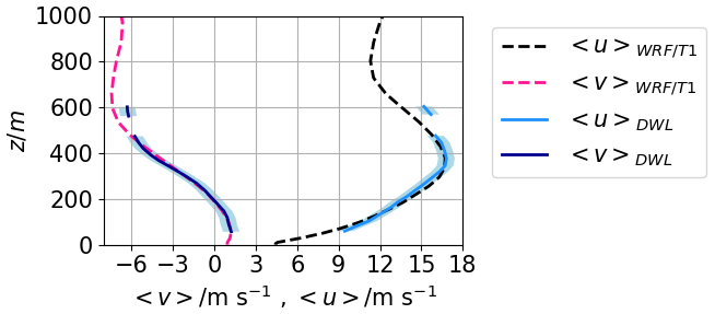
Figure 1 Vertical profiles of the measured velocities at the WiValdi site (zonal 〈u〉_DWL, meridional 〈v〉_DWL; shaded areas indicate the DWL uncertainty of ±0.5 m s⁻¹) and the continuous profiles from the WRF simulations used as target profile T1 (zonal $\langle u{\rangle }_{\mathrm{WRF}/\mathrm{T}\mathrm{1}}$, meridional $\langle v{\rangle }_{\mathrm{WRF}/\mathrm{T}\mathrm{1}}$).

2.4 Numerical setup

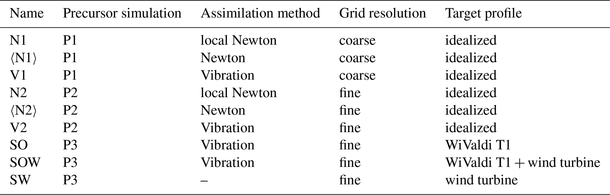
Table 1 gives an overview of all simulations performed in this study. Figure 2 shows a schematic illustration of the simulation approach used in this study. The numerical simulations are separated into precursor simulations (P1, P2, and P3 in Fig. 2) and simulations with data assimilation (N1, 〈N1〉, V1, N2, 〈N2〉, V2, and SO in Fig. 2) (+ wind turbine simulations, SW and SOW in Fig. 2). A precursor simulation is necessary so that characteristic atmospheric turbulence can spin up in the computational domain. The precursor simulations P1, P2, and P3 employ periodic lateral boundary conditions and are run until a fully developed turbulent state prevails. In the subsequent simulations, in which the output of the precursor simulations is used as the inflow field, either the local Newtonian relaxation according to Eq. (4) (N1, N2), the Newtonian relaxation according to Eq. (6) (〈N1〉, 〈N2〉), or the vibration method using Eq. (7) (V1, V2, SO) is applied.

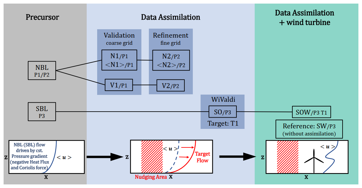
Figure 2 Schematic illustration of the different simulations considered in this study. The abbreviations indicate the simulation type following Table 1.

Our numerical simulations N1, 〈N1〉, and V1 have a similar setup as those of Nakayama and Takemi (2020). N1 and V1 and are conducted to verify the correct implementation of our assimilation methods and 〈N1〉 to investigate the effects of the Newtonian method in the presented setup with a nudging region. The sensitivity of the different assimilation methods to grid refinement is evaluated with the simulations N2, 〈N2〉, and V2. The assimilation towards more complex target profiles for the zonal and meridional velocity components is tested in the simulation SO. As mentioned above, these profiles are close to observations at the wind farm site WiValdi (Fig. 1). While we have tested different Newtonian relaxation timescales (τ=30 s, τ=60 s, and τ=300 s) and different vibration frequencies (f₀=0.002 s⁻¹, f₀=0.005 s⁻¹, and f₀=0.01 s⁻¹), in this study only the results for τ=30 s and f₀=0.002 s⁻¹ are shown. These particular values led to the closest alignment with the target profile.

2.4.1 Idealized cases – coarse resolution (P1, N1, 〈N1〉, V1)

In the precursor simulation P1, a fully developed flow corresponding to an NBL with the zonal velocity profile $u=\frac{u_{*}}{\mathit{\kappa }}\ln \left(\frac{z}{z_{\mathrm{0}}}\right)$ (friction velocity $u_{*}=\mathrm{0.45}$ m s⁻¹, roughness length z₀ = 0.1 m, von Kármán constant κ = 0.4) is achieved by the application of a constant pressure gradient in the horizontal direction, following Nakayama and Takemi (2020). In Fig. 2, P1 refers to this precursor simulation. The pressure gradient is implemented as an additional forcing $-u_{*}^{\mathrm{2}}/H$ in Eq. (2) with the abovementioned friction velocity and the domain height H = 1000 m. For the surface friction the drag coefficient in the surface parameterization is set to 0.017, which is a requirement of EULAG's Neumann boundary conditions. The domain size is $\mathrm{6000}\times \mathrm{6000}\times \mathrm{1000}$ m³ with a grid spacing of dx=dy = 40 m and dz=10 m. 150 000 time steps with Δt = 1 s are calculated on 100 processors in 25 h for this precursor simulation to develop a statistically stable state.

The precursor simulation is performed with periodic boundary conditions in the horizontal directions and a rigid lid at the top of the domain. The Coriolis parameter is set to zero. For the following simulation with data assimilation, synchronized 2D yz slices are extracted at x = 3000 m at each time step after the simulation has reached a quasi-equilibrium state. A total of 1050 2D slices of the three velocity components and the potential temperature perturbation were taken as input at the inlet of the nudging simulation.

The nudging simulations N1, 〈N1〉, and V1 are calculated with periodic boundaries in the meridional y direction, an open boundary condition at the zonal outflow in the x direction, and a gradient-free, rigid-lid upper boundary. The Coriolis term in Eq. (2) is omitted in the nudging simulations, which is different to the setup of Nakayama and Takemi (2020). An explanation for this difference is given in Sect. 3. A nudging zone is introduced from x = 1.0–2.0 km over the whole lateral and vertical span of the computational domain. A logarithmic zonal target wind profile with $u_{*}=\mathrm{0.41}$ m s⁻¹ and z₀=0.2 m is assumed, while the meridional target wind profile is set to 0. The three assimilation methods (Eqs. 4, 6, 7) are tested separately for the adaption towards the zonal target profile in N1, 〈N1〉, and V1, respectively. Numerical absorbers (the term F_abs in Eq. 2) are included at the top above z = 700 m with α=200 s and at the outflow for x>5000 m with α=30 s according to Smolarkiewicz et al. (2007) in order to attenuate the solution to the prescribed states in proximity to the open boundaries (cf. Smolarkiewicz et al., 2007).

2.4.2 Idealized cases – fine resolution (P2, N2, 〈N2〉, V2)

As wind turbine simulations, especially in stably stratified regimes, are commonly computed with a higher resolution in order to resolve a large part of the turbulent structures we performed a precursor simulation P2 for the same NBL conditions as in P1 with a grid spacing of $\mathrm{d}x=\mathrm{d}y=\mathrm{d}z$ = 5 m. The time step has to be decreased to Δt = 0.2 s, and a smaller domain of $\mathrm{6000}\times \mathrm{3000}\times \mathrm{1000}$ m³ is chosen in order to reduce the calculation time. The boundary conditions remain the same as in the coarse grid equivalent. The drag coefficient is set to 0.01, which leads to a vertical profile described in Sect. 2.4.1 after the simulation has reached a statistically stable state. Due to the smaller time step, a total of 6000 synchronized 2D yz slices are extracted from this precursor simulation for the input of the nudging simulations N2, 〈N2〉, and V2. With this high-resolved inflow the performance of the assimilation techniques Eqs. (4), (6), and (7) can be investigated. All other settings in N2, 〈N2〉, and V2, not referred to in this paragraph, are identical to N1, 〈N1〉, and V1.

2.4.3 More realistic cases (P3, SO, SOW, SW)

In Sect. 5 a more complex target profile is implemented which has a zonal and a meridional component close to the measurements at the wind farm site WiValdi (Fig. 1). Therefore, a third precursor simulation P3 is introduced with dominant wind shear and veer in the ABL flow. The atmospheric condition in this simulation corresponds to a stable stratification. This precursor simulation was developed by Englberger and Dörnbrack (2018) during their investigation of the impact of different thermal stratifications on wind turbine wakes. The domain size in the simulations applying the precursor simulation P3 is $\mathrm{5120}\times \mathrm{2560}\times \mathrm{430}$ m³ with a grid spacing of $\mathrm{d}x=\mathrm{d}y=\mathrm{d}z=\mathrm{5}$ m in the lowest 200 m. Above 200 m the vertical spacing is dz=10 m. For the simulation SO with nudging, the nudging zone is inserted at x = 1.0–2.0 km and an absorber is included for x > 4520 m with α=30 s. Due to the fact that in an SBL negative buoyancy diminishes vertical mixing no damping layer is included at the domain top. In the corresponding wind turbine simulation SOW the NREL 5 MW rotor is placed 200 m downstream of the nudging zone, which is included from 0.5–1.5 km. The calculation time of the wind turbine simulation is 60 min with an averaging period of the velocities of 20 min at the end of the simulation. A reference simulation SW with the wind turbine is computed with the original precursor P3 as inflow without an assimilation approach.

The assimilation methods described in Sect. 2.2 are only suitable if the domain-averaged mean flow of the precursor simulation corresponds to the height-averaged target value. This is required to preserve mass continuity (Eq. 1) in the numerical model. If there is a difference between the precursor and the target velocity profile, the horizontal mean of the vertical profile of the precursor simulation has to be normalized:

$$\begin{array}{}\text{(8)}& v_i^{\mathrm{new}}(x,y,z)=\mathit{\alpha }\langle {\stackrel{\mathrm{‾}}{v}}_i^p\left(z\right){\rangle }_{x,y}+v_i^{\prime p}(x,y,z)\end{array}$$

with

$$\begin{array}{}\text{(9)}& \mathit{\alpha }={\displaystyle \frac{\langle v_{i,\mathrm{OBS}}{\rangle }_z}{\langle {\stackrel{\mathrm{‾}}{v}}_i^p{\rangle }_{x,y,z}}}.\end{array}$$

Here, $v_i^{\mathrm{new}}$ is the new velocity value of the inflow field at every grid point, $\langle {\stackrel{\mathrm{‾}}{v}}_i^p\left(z\right){\rangle }_{x,y}$ is the spatial (〈〉_x,y) and time-averaged mean value at every height of the precursor simulation, and $v_i^{\prime p}=v_i^p-\langle {\stackrel{\mathrm{‾}}{v}}_i^p\left(z\right){\rangle }_{x,y}$ is the fluctuation at every grid point i,j, and k of the precursor simulation. α is derived from the division of the mean of the target profile 〈v_i,OBS〉_z (averaged over the height of the ABL) by the time- and volume-averaged mean velocity (averaged over the last 20 min) of the precursor simulation $\langle {\stackrel{\mathrm{‾}}{v}}_i^p{\rangle }_{x,y,z}$.

The magnitude of the inflow field from P3 for the simulation with data assimilation SO has been modified according to Eq. (8) with α = 1.25 (α = 0.4) for the zonal (meridional) velocity components.

Table 1 Simulations conducted in this study.

2.5 ABL and wind turbine characteristics

In this work the following characteristics of the ABL are investigated:

• The mean vertical profiles of the zonal (〈u(x_a,z)〉_y) and meridional velocities (〈v(x_a,z)〉_y) are calculated at each height level at certain downstream positions x_a averaged in the y direction 〈〉_y.

• The resolved mean TKE of the ABL,

  $$\begin{array}{}\text{(10)}& \begin{array}{rl}\langle \mathrm{TKE}(x_{\mathrm{a}},z){\rangle }_y& ={\displaystyle \frac{\mathrm{1}}{\mathrm{2}}}\langle (\langle u^{\prime }(x_{\mathrm{a}},y,z{)}^{\mathrm{2}}{\rangle }_y\\ & +\langle v^{\prime }(x_{\mathrm{a}},y,z{)}^{\mathrm{2}}{\rangle }_y\\ & +\langle w^{\prime }(x_{\mathrm{a}},y,z{)}^{\mathrm{2}}{\rangle }_y){\rangle }_y,\end{array}\end{array}$$

  is calculated at each height level at a certain downstream position x_a averaged in the y direction 〈〉_y. u^′, v^′, and w^′ are the turbulent fluctuations of the velocity components u, v, and w. The fluctuations are calculated by subtracting the y-averaged mean velocities from the instantaneous value at each height level. Here, ${\mathit{\chi }}^{\prime }(x_{\mathrm{a}},y,z)=\mathit{\chi }(x_{\mathrm{a}},y,z)-\langle \mathit{\chi }(x_{\mathrm{a}},z){\rangle }_y$ with $\mathit{\chi }=(u,v,w)$.

• The horizontal energy spectrum is calculated according to Stull (2003, Chap. 8.6).

Concerning the wind turbine simulations in Sect. 6 the time-averaged zonal velocity component $\stackrel{\mathrm{‾}}{u_{i,j,k}}$ is shown, which is averaged over the last 20 min of the simulation. The zonal velocity deficit is calculated with

$$\begin{array}{}\text{(11)}& {\mathrm{VD}}_{i,j,k}\equiv {\displaystyle \frac{\stackrel{\mathrm{‾}}{u_{i_{\mathrm{0}},j,k}}-\stackrel{\mathrm{‾}}{u_{i,j,k}}}{\stackrel{\mathrm{‾}}{u_{i_{\mathrm{0}},j,k}}}}.\end{array}$$

Here, $\stackrel{\mathrm{‾}}{u_{i_{\mathrm{0}},j,k}}$ corresponds to the velocity 200 m upstream of the wind turbine in the x direction.

3 Results: data assimilation with coarse grid resolution

In this section the test scenario proposed by Nakayama and Takemi (2020) with a grid spacing of $\mathrm{d}x=\mathrm{d}y=\mathrm{40}$ m and dz=10 m is reproduced in EULAG with the three different assimilation techniques described above. The aim of this section is to verify that there are no major differences in the numerical results and that EULAG is able to reproduce similar findings like in the work of Nakayama and Takemi (2020). The results with coarse resolution are also necessary to enable a comparison with the results with a finer grid (Sect. 4) and they are a verification for our numerical setup without Coriolis force, which differs from Nakayama and Takemi (2020).

The results of both types of Newtonian relaxations (Eqs. 4 and 6) and the assimilation method using the vibration equation (Eq. 7) are shown in Fig. 3. Vertical profiles of the zonal velocity and the resolved TKE at different downstream positions are presented. The zonal velocity component is adapted precisely towards the target profile for the two options of the Newtonian relaxation (Fig. 3a and b). A slight overestimation of the target velocity profile by less than 0.5 m s⁻¹ can be seen for the simulation with the vibration method (Fig. 3c). In all simulations, the flow downstream of the nudging zone does not change considerably at the positions x=2 km, x=3 km, and x=4 km. The meridional velocity component is approximately zero in the precursor simulation and is not changed inside the nudging zone (not shown).

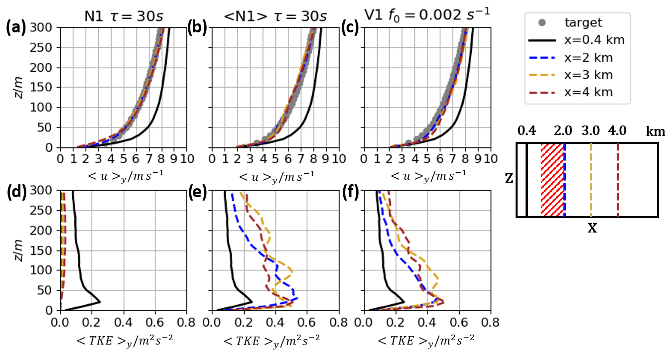
Figure 3 Results for the simulations N1, Eq. (4) and 〈N1〉, Eq. (6) with τ = 30 s and V1, and Eq. (7) with f₀ = 0.002 s⁻¹. Vertical profiles of the zonal velocities 〈u〉_y in (a), (b), and (c) and the 〈TKE〉_y in (d), (e), and (f) for different downstream positions. The black solid lines show the quantities for the upstream flow at x=0.4 km. The gray dotted lines represent the target wind profile. The blue (gold, brown) lines refer the downstream positions x=2 km (x=3 km, x=4 km). The scheme on the right side indicates the downstream positions for the evaluation (the red hatched area refers to the nudging zone).

Regarding the TKE, a strong damping to values below 0.05 m² s⁻² can be seen at all heights shown when the local Newtonian relaxation according to Eq. (4) is applied (Fig. 3d). Sensitivity studies reveal that a relaxation time longer than the 30 s used here leads to smaller turbulence damping but to a poorer adjustment to the target velocity profile (not shown). This result is in agreement with previous findings by Neggers et al. (2012).

With the Newtonian relaxation represented by Eq. (6) instead, the TKE is 2.5 to 3 times higher when compared to the upstream values (Fig. 3e). From this result it is concluded that TKE is not damped if the applied forcing of the assimilation method acts on the mean flow field 〈v〉 in Eq. (6) and not on the local velocity values at each grid point as in Eq. (4). The TKE is also larger than upstream of the nudging zone when the vibration method is used (Fig. 3f) with values up to 2 times higher. In particular, above z=150 m the increase in TKE is not as large in V1 (max. 0.18 m² s⁻²) when compared to 〈N1〉 (max. 0.25 m² s⁻²).

In summary, similar conclusions can be drawn comparing the results in the presented study with the results from Nakayama and Takemi (2020). EULAG successfully reproduces the assimilation of the zonal velocity component towards the target profile with all three tested methods. Concerning the TKE profiles, the local Newtonian relaxation according to Eq. (4) leads to a destruction of TKE, while the simulated resolved turbulence is increased for the Newtonian relaxation and the vibration method at all positions downstream of the nudging zone (when compared to the inflow TKE). The overestimation of the original TKE if the Newtonian method is applied is comparable to the results of Allaerts et al. (2020, 2023) where they applied the relaxation technique in the whole domain in the precursor simulation. Our results using the vibration method are similar to those of Nakayama and Takemi (2020). Both methods increase the TKE in the simulated neutral case.

Although similar conclusions can be drawn comparing the results in this study with the work of Nakayama and Takemi (2020), there are differences in the flow fields downstream when implementing the Coriolis force, as they do in their setup. Without Coriolis force, a restoring of the non-assimilated upstream flow downstream of the assimilation region does not occur in our simulations, whereas it does in Nakayama and Takemi (2020). One possible reason could be their inclusion of the Coriolis force. When the Coriolis force was included in our EULAG simulations, the flow evolved temporally beyond the nudging zone away from the target profile as the Coriolis forces are applied to velocity perturbations, which are large beyond the nudging zone (Eq. 2).

4 Results: data assimilation within highly resolved idealized simulations

In order to resolve smaller turbulent structures and motions, LESs with a higher resolution than that used in Sect. 3 are performed in this part of the study. As the power output and performance of a wind turbine are impacted directly by the atmospheric turbulence it is crucial to resolve a large part of the turbulent spectra in order to simulate the interaction of the rotor blades with the flow more precisely. Hence, the implemented assimilation methods need to be tested for higher-resolved simulations with a grid spacing of $\mathrm{d}x=\mathrm{d}y=\mathrm{d}z=\mathrm{5}$ m (N2, 〈N2〉 and V2 in Fig. 2), i.e., with grid sizes that are often used in wind turbine LESs (e.g., Vollmer et al., 2016; Englberger and Dörnbrack, 2018; Chanprasert et al., 2022). In this section, we extend the work of Nakayama and Takemi (2020) and investigate the assimilation methods on a finer resolved grid.

Figure 4a–f show vertical profiles of the zonal velocity and TKE at different downstream positions for all three tested assimilation methods. This figure is directly comparable to the results of the corresponding coarse-resolution simulations shown in Fig. 3. Figure 4g–i present in addition the spectral energy distribution S(k) as a function of the wave number $k=\mathrm{1}/\mathrm{\ell }\left(x\right)$, where ℓ(x) is the length ranging from 2dx to 500 m. The horizontal power spectra at z=90 m are averaged over the y direction and are presented for the flow upstream of, inside, and downstream of the nudging zone.

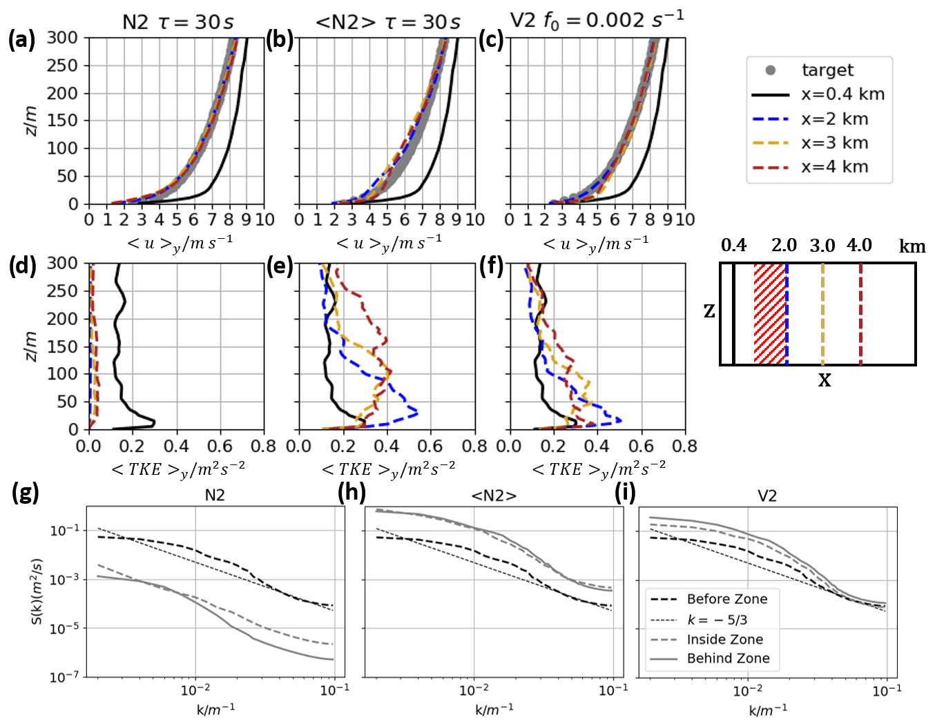
Figure 4 Results for the simulations with Newtonian relaxation N2 (Eq. 4, τ=30 s) and 〈N2〉 (Eq. 6, τ = 30 s) and the vibration method V2 (Eq. 7, f₀ = 0.002 s⁻¹) with the fine grid resolution. Vertical profiles of the zonal velocities 〈u〉_y in (a), (b), and (c) and the 〈TKE〉_y in (d), (e), and (f). The black solid lines show the quantities for the upstream flow at x=0.4 km. The gray dotted lines show the target wind profile. The blue (gold, brown) lines refer to the results for x = 2 km (x=3 km, x=4 km). The scheme on the right side indicates the downstream positions for the evaluation. In (g), (h), and (i) the horizontal spectra (z=90 m, length 500 m, width 3000 m) for each simulation are shown for the flow before (black dashed), inside (gray dashed), and downstream (gray solid) of the nudging zone.

Starting with the local Newtonian relaxation, the zonal velocity is assimilated precisely towards the target profile for simulation N2 (Eq. 4) and does not change after the relaxation zone at x=3 km or x=4 km (Fig. 4a). For this case, however, the TKE is decreased to values below 0.05 m² s⁻² inside the nudging zone and further downstream. From this result, we deduce that the effect of local Newtonian relaxation on small-scale turbulence is not resolution-dependent, since this is the same finding as in the corresponding coarse-resolution simulation N1.

In contrast, when the Newtonian relaxation is applied in simulation 〈N2〉 (Eq. 6), the target velocity profile is underestimated by 0.8 m s⁻¹ at x=2 km and z=50 m. At higher altitudes, the x=2 km profile is consistent with the target profile (Fig. 4b). Further downstream, at x=3 km and x=4 km, the velocity still correlates well with the target profile within a tolerance of 0.5 m s⁻¹. The TKE in this case is 2–3 times higher downstream of the nudging zone than in the upstream flow (Fig. 4e). The assimilation to the target profile in simulation 〈N2〉 (Fig. 4b) is slightly worse than in simulation 〈N1〉 (Fig. 3b), and the TKE is affected in the same way (Figs. 3e and 4e), which means that there is no dependence on the resolution when using the Newtonian relaxation as an assimilation method in the presented setup.

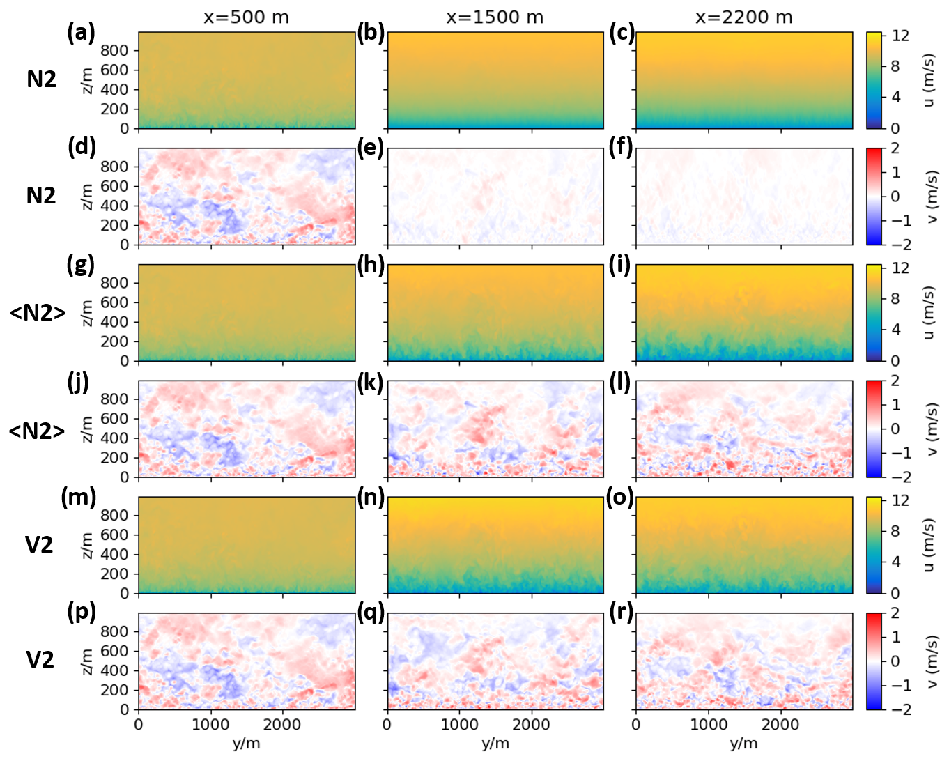
Figure 5 Vertical cross-sections of the zonal and the meridional velocity u and v for x=500 m upstream, x=1500 m inside, and x=2200 m downstream of the nudging zone. The results are shown for the simulations N2 (a–f), 〈N2〉 (g–l), and V2 (m–r).

To gain more detailed insight into the effects of the forcings applied in the simulations N2 (Eq. 4) and 〈N2〉 (Eq. 6) on the flow field, lateral cross-sections of instantaneous u and v fields are presented in Fig. 5a–l. The inflow fields at x=500 m are the same for the two simulations shown in Fig. 5a and g and they basically represent the flow field of the precursor simulation P2. In the relaxation region, however, there is a striking difference between local Newtonian and Newtonian relaxation method (Fig. 5b and h). While in both cases the absolute value of the u field is adjusted to the target profile by a deceleration of the mean flow, the flow field in simulation 〈N2〉 (Fig. 5h) is still turbulent and no laminarization occurs, as it is the case in the simulation N2 (Fig. 5b).

The same difference can be observed for the v components (Fig. 5e and k). The turbulent structures of v are not significantly altered within the relaxation region in simulation 〈N2〉 (Fig. 5k), while they are strongly suppressed in simulation N2 (Fig. 5e). This behavior in the relaxation region at x=1500 m is similar for the downstream position x=2200 m. From Fig. 5 it can be concluded that the turbulent structure of the eddies in the simulation domain are severely affected by the local Newtonian method, while the Newtonian relaxation and the vibration method seem to be less intrusive.

The above finding is supported by analyzing the spectra (Fig. 4g–h). In the case of the local Newtonian relaxation in simulation N2, the spectral energy density before the nudging (in P2) is much higher. This local Newtonian relaxation basically reduces the energy on all scales in the whole domain, resulting in a strongly reduced value of S(k) to less than 10 % of the inflow energy in Fig. 4g in comparison to Fig. 4h in simulation 〈N2〉. Applying the Newtonian relaxation in simulation 〈N2〉, the spectral energy density increases on all scales. This finding is in agreement with the increase in the resolved TKE (Fig. 4e).

In the following, the application of the vibration method and the comparison of the corresponding simulation V2 with the simulation 〈N2〉 of the Newtonian relaxation are presented in order to investigate the difference of these two different methods on a fine grid. The vertical profile of the zonal velocity results in an exact adjustment to the target profile at x=2 km (Fig. 4c). Only at z = 20 m is the actual velocity component slightly overestimated compared to the target profile at x=3 km and x=4 km. At all other heights, the simulated velocities overlap nearly perfectly with the target profile. Figure 4f shows the vertical profiles of TKE. The TKE at the downstream positions is 1.5–2 times higher than in the upstream flow beneath z = 150 m. Above z = 150 m, there is only a small deviation between the downstream and upstream TKE (±0.06 m² s⁻²).

The vibration method leads to a more precise assimilation towards the target profile in the fine grid case of simulation V2 in comparison to the coarse grid simulation V1 (compare Figs. 3c and 4c). Furthermore, the impact of the vibration method on the TKE is less pronounced for the fine grid simulation (Fig. 4f) than in the coarse grid simulation (Fig. 3f), suggesting that the vibration method performs better with higher resolution.

The impact of the different forcings f in Eq. (2) due to the Newtonian relaxation (Eq. 6) and due to the vibration method (Eq. 7) on the instantaneous flow field is presented in Fig. 5g–r for both u and v components of simulations 〈N2〉 and V2. In general, the turbulent structure is very similar in both simulations. This could be interpreted to reflect the fact that both assimilation methods basically impact the horizontal mean (Fig. 4b and c) and, consequently, the resolved TKE (Fig. 4e and f). However, the turbulent 2D flow structure in Fig. 5i, l, o, and r is only affected to a small extent. The increase in turbulence – especially below 150 m height – within and after the nudging zone compared to the region in front (Fig. 4e–f) is partly due to an increase in $\frac{\mathrm{\Delta }u}{\mathrm{\Delta }z}$ in the target profile in comparison to the inflow profile of P2. It is also partly an effect of the Newtonian relaxation itself, as the v contribution to the TKE is also larger in simulation 〈N2〉 in comparison to simulation V2, whereas $\stackrel{\mathrm{‾}}{v}=\mathrm{0}$ in both cases (not shown).

For a more detailed comparison between the Newtonian and the vibration approach, the spectral energy density is shown in Fig. 4h–i for simulations 〈N2〉 and V2. On large scales (small wave number k), the spectral power S(k) increases similarly behind the nudging zone. In the nudging zone, however, the vibration method does not instantaneously reach the final spectral energy density observed behind the nudging zone. The transition occurs not as abruptly as in simulation 〈N2〉. This abrupt transition could be an effect of the Newtonian relaxation itself applied in 〈N2〉, which is also responsible for the higher TKE in Fig. 4e in comparison to Fig. 4f. Further, going to smaller scales (larger wave number k), the impact of the vibration method on the energy spectra decreases and for k>0.04 m⁻¹ an equal energy level can be seen. This is also different in comparison to the behavior of simulation 〈N2〉.

All tested methods assimilate the mean flow to the target profile reasonably well. The local Newtonian relaxation method applied in N1 and N2 is not applicable for wind turbine applications, as the TKE of the assimilated flow fields is significantly reduced and the flow becomes nearly laminar. It is clear that in both the vibration method and the Newtonian relaxation method, turbulence still persists after assimilation to a given target velocity profile in comparison to the local Newtonian approach, in which a laminarization occurs. In both assimilation methods the flow is more turbulent than the inflow profile, meaning that both methods add additional turbulence. Including the spectral analysis, the integral approach of the vibration method leads to a more gentle adjustment of the energy content, while the wind profiles adjust similarly well in both approaches. The resolution impact in the case of the Newtonian relaxation methods is only weakly pronounced, while the vibration method shows improved results for an increased resolution.

The coarse- and fine-resolution results show a very similar behavior of the resulting flow field using the Newtonian and the vibration approach. The investigations in this section for the higher grid resolution show an improved capability of the vibration method – compared to the simulations in the coarser grid – to assimilate the mean zonal velocity component, while the impact on the TKE is smaller. Compared to the Newtonian relaxation the impact on the TKE is also less dominant when the vibration approach is applied. The following simulations, which perform an assimilation to observed profiles from the WiValdi wind park, are conducted by using the vibration method only, as, to our knowledge, this method has not been previously tested for wind-turbine-relevant resolutions. It has to be emphasized that our approach includes a nudging region smaller than the numerical domain and omits the Coriolis force term in the simulation with active additional forcing due to the assimilation methods. However, within the scope of interest to generate an inflow situation for a single wind turbine with small domain sizes and short simulation times, we are convinced that the presented model setup is a first step towards this final goal.

The performance of the Newtonian relaxation and possible adaptions in the model are investigated by Allaerts et al. (2020, 2023) for an assimilation which is implemented as a grid-nudging method acting on every grid point in the domain, while an active Coriolis force term and pressure gradient lead to a geostrophic equilibrium in the simulation. They also investigated the vibration method, but only in combination with the Newtonian approach, with no significant difference in the behavior of their algorithm (Allaerts et al., 2020).

5 Results: assimilation towards a zonal and a meridional target profile measured in an SBL at the wind farm site WiValdi

The previous section has presented the efficient assimilation of the zonal velocity component in an NBL towards an idealized target wind profile for a grid spacing of $\mathrm{d}x=\mathrm{d}y=\mathrm{d}z=\mathrm{5}$ m. In this section, a more complex stably stratified situation is considered with an assimilation of both the zonal and the meridional wind component towards a wind profile from a WRF simulation (cf. Appendix A). As mentioned above in Sect. 2.3, these profiles are close to measured velocity profiles from the wind farm site WiValdi (Fig. 1) and provide continuous target profiles at each height of the domain. The objective of the simulation SO (cf. Fig. 2) is the generation of a more realistic inflow field for a wind turbine simulation, which will be discussed in Sect. 6. This test case in an SBL presents a preliminary step towards the application of the vibration method with the developed setup using a nudging zone in front of a wind turbine.

The data assimilation is more complex, as both the zonal and the meridional components have to be adjusted to the target profiles. This extends the work of the previous section where the assimilation was only applied to the zonal velocity component. Hence, the simulation SO is a step towards more realistic inflow fields guided by observational data. As described above, the vibration method is used in the following for the adjustment towards the WiValdi profile.

In a first approach (not shown), we tested if the velocities of the neutral precursor simulation P2 could be assimilated towards the target profiles $\langle u{\rangle }_{\mathrm{WRF}/\mathrm{T}\mathrm{1}}$ and $\langle v{\rangle }_{\mathrm{WRF}/\mathrm{T}\mathrm{1}}$ from Fig. 1. However, the meridional velocity component in P2 is close to zero over the whole boundary layer height, while the target profile has positive values below z=200 m and decreases above until −7 m s⁻¹ at z=600 m. This strong veer of the flow in the target profile contrasts with the pure zonal flow in P2. The assimilation of the flow in P2 towards the new target profile created numerical artifacts.

For this reason, we use another precursor simulation P3 of a stable boundary layer from Englberger and Dörnbrack (2018), which has been introduced in Sect. 2.4. Wind shear and, in particular, wind veer both occur in this boundary layer flow. Figure 6a–b show the mean velocities 〈u〉_y and 〈v〉_y of the modified precursor simulation for the SBL in comparison to the target velocity profiles. The results for the assimilated velocities and the TKE are shown in Fig. 6 for the inflow and the positions x=2, 3, and 4 km downstream of the nudging zone.

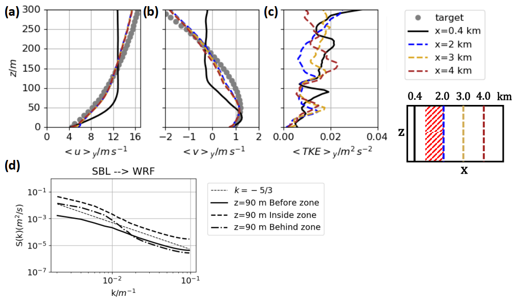
Figure 6 Results for SO of the assimilation towards the representative WRF velocity profile with the precursor simulation P3 and application of the vibration method (f₀=0.002 s⁻¹). (a) Zonal velocity 〈u〉_y, (b) meridional velocity 〈v〉_y, and (c) 〈TKE〉_y. The black solid lines refer to the values upstream of the nudging zone. The gray dotted lines in (a) and (b) indicate the zonal and meridional target velocity profile T2. The colored lines show the values for the downstream positions according to the scheme on the right. In (d) the horizontal energy spectra are shown for the height z=90 m (length 500 m, width 3000 m) for the flow before, inside, and behind the nudging zone.

With a frequency of f₀=0.002 s⁻¹ in the vibration method an assimilation towards the target zonal profile is achieved beneath z=150 m with a slight overestimation of <0.3 m s⁻¹ (Fig. 6a). Above z=150 m, the zonal target is underestimated by up to 1 m s⁻¹. Figure 6b shows that the meridional velocity component can be adapted to the target profile with a slight underestimation (overestimation) of less than 0.35 m s⁻¹ between z=50 m and z=150 m (z=240 m and z=300 m).

Regarding the TKE, shown in Fig. 6c, it can be seen that the turbulent regime is mostly unchanged due to the vibration method at the downstream positions. Over the whole boundary layer height the TKE stays within a range of ±0.01 m² s⁻². The spectral analysis in Fig. 6d shows the spectral energy S(k) at z=90 m, which is close to the hub height of the wind turbine in WiValdi. Similar to the neutral simulation V2, the assimilation increases the spectral energy at large scales. At small scales (large k values), the spectral energy is similar upstream and downstream of the relaxation zone.

A visualization of the u and v components of the flow for a cross-section before, inside, and downstream of the nudging zone is presented in Fig. 7. In general, the upstream flow (Fig. 7a and d) is less turbulent compared to the NBL in the previous section (e.g., Fig. 5a and d), which is a typical characteristic of the SBL, as the only turbulence source is shear close to the surface. The adjustment of the u and v components is clearly visible for the downstream positions, while the turbulent structures are not affected considerably (Fig. 7b, c, e, f). The zonal flow component is decelerated below 150 m in height and accelerated above. The vibration method lifts the sign-changing height of the meridional velocity component v from 100 to 200 m. It further increases the gradient at this transition zone, while the 2D turbulent structure of v is not considerably changed by this process. This pattern also prevails at the wind turbine position, downstream of the nudging zone.

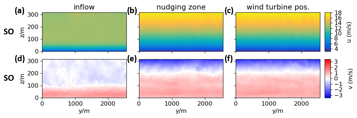
Figure 7 Vertical cross-sections of the zonal and the meridional velocity u and v for the inflow area before the nudging zone (a, d), the outflow of the nudging zone (b, e), and downstream of the nudging zone at the wind turbine position (c, f). The results are shown for the simulation SO.

In summary, the wind profiles of the SBL could be adjusted efficiently towards the representative WRF velocity profiles using the vibration method. Obviously, a successful data assimilation requires that the target profiles, which prescribe wind shear and veer, are approximated by a precursor simulation with similar characteristics. Furthermore, it is remarkable that the resolved TKE in the SBL is less overestimated downstream of the nudging zone compared to the idealized neutral cases presented in Sect. 4.

The considered test case of the assimilation of the horizontal velocity components in an SBL shows that the velocities do not change considerably as the flow propagates further downstream of the nudging zone, which was an unresolved issue in the setup presented by Nakayama and Takemi (2020). With the presented simulation SO which omits the Coriolis force term and applies the vibration method in a nudging zone the inclusion of a wind turbine at a downstream position after the relaxation zone seems to be reasonable. This will be presented in the next section.

6 Results: analysis of the wind turbine wake for an assimilated atmospheric inflow

In this section the simulation SO presented in the previous section is repeated with the integration of an NREL 5 MW wind turbine (h_hub=90 m, D=126 m), located downstream of the nudging zone (SOW in Fig. 2). The wind turbine rotor is modeled in EULAG according to the parameterization presented in Sect. 2.1 and is located at x=1700 m, i.e., 200 m downstream of the nudging zone (from 0.5–1.5 km in SOW).

Additionally, a reference simulation SW has been computed with the wind turbine exposed to the original SBL precursor simulation P3 in order to analyze the differences in the developed wakes. With this implementation an efficient testing of different target wind profiles and hence different inflow fields for a wind turbine could be achieved. Showing the applicability of this approach is the objective of this section.

The time-averaged (over the last 20 min of the simulation) zonal velocity component for both cases is shown for three x–y planes covering hub height (z=90 m) as well as the upper (z=120 m) and lower rotor half (z=60 m) of the NREL 5 MW rotor in Fig. 8. The influence of the assimilation method on the zonal velocity is clearly visible in Fig. 8d, e, and f. The inflow velocities in front of the wind turbine are reduced towards the target wind profile (cf. Fig. 6a). Furthermore, the wake is deflected northwards in the assimilated simulation due to the increased vertical gradient of the meridional velocity over the upper rotor half (cf. Fig. 6b). In contrast, the wake in the reference simulation is only deflected in the lower part of the rotor (Fig. 8c) because wind veer only occurs in the lowest 100 m of the boundary layer in P3 (cf. Fig. 6b, black curve). Furthermore, the deflection in the simulation SW is not as pronounced as in SOW, as the meridional wind component is smaller (v_SW(60 m)<v_SOW(60 m)).

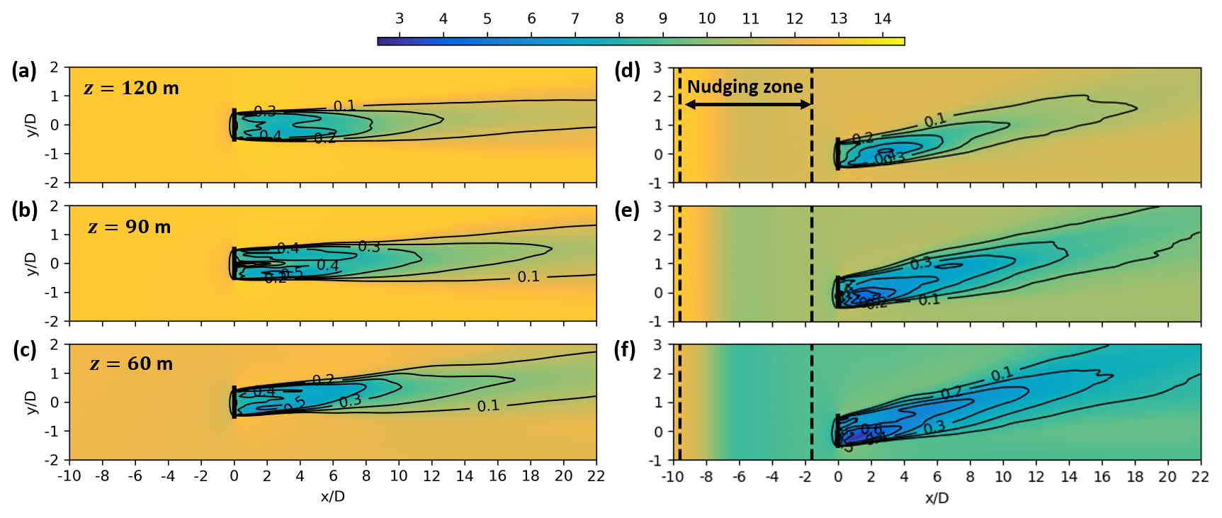
Figure 8 Colored contours of the time-averaged zonal velocity component $\stackrel{\mathrm{‾}}{u_{i,j,k}}$ in m s⁻¹ for SW in (a), (b), and (c) and for SOW in (d), (e), and (f) averaged over 20 min at the end of the simulation. Panels (b) and (e) show the x–y plane at hub height z=90 m. Panels (a) and (d) (c and f) correspond to the x–y planes at $Z=\mathrm{90}\mathrm{m}+R/\mathrm{2}=\mathrm{120}$ m ($Z=\mathrm{90}\mathrm{m}-R/\mathrm{2}=\mathrm{60}$ m). The black contours represent the velocity deficit $V{D}_{i,j,k}$ at the same vertical location calculated in relation to the upstream velocity at $x=-\mathrm{200}$ m. The axes are normalized by the rotor diameter D=126 m, whereby $x/D=\mathrm{0}$ indicates the position of the rotor.

The streamwise wake extension is similar in both cases at z=60 m and z=90 m. A reduced wake extension is seen at z=120 m for the assimilated case (Fig. 8d). In simulation SOW, the zonal velocity deficit of 10 % is reached at $x/D=\mathrm{18}$ in comparison to $x/D=\mathrm{22}$ in the simulation without assimilation SW (Fig. 8a). However, higher velocity deficit values are reached at similar downwind distances (20 % at $x/D$ = 10–12).

One reason for the reduced wake extension is the higher entrainment in the upper part of the rotor due to significantly increased vertical gradients of the zonal and meridional velocity components (Fig. 6a and b). Another reason is the pitch angle of the blades, which is 3.5° for a hub height wind speed of $\stackrel{\mathrm{‾}}{u}$ = 12–13 m s⁻¹ in simulation SW, while it is 0° for $\stackrel{\mathrm{‾}}{u}<\mathrm{12}$ m s⁻¹ in simulation SOW. The blades of the wind turbine in the assimilated flow field impose higher tangential and axial forces on the flow field. Further, these reasons are also responsible for the maximum velocity deficit difference in the near wake. It is 60 % in simulation SOW in Fig. 8e and f, while it reaches only 50 % in simulation SW in Fig. 8b and c.

Figure 9a and c show the lateral view of a vertical plane through the center of the wind turbine with the visualization of the time-averaged zonal velocity component $\stackrel{\mathrm{‾}}{u}$. Figure 9b and d present a downstream view of the wake at x=5 D behind the rotor. Only a part of the wake is seen in Fig. 9c due to the deflection of the wake out of this x–z plane. While the meridional wind component was predominant only in the lower section of the rotor in the reference case (Fig. 9b) the assimilated wind veer (cf. Fig. 6b) leads to a deflection of the wake over the whole rotor height in the simulation SOW (Fig. 9d). In both cases, the wakes respond to the prevalent veer with a stretching of the wake from a circular-shaped one towards an ellipsoidal-shaped one, which is characteristic under veering inflow conditions.

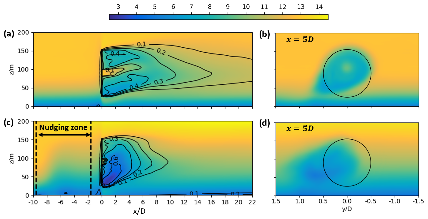
Figure 9 Colored contours of the time-averaged zonal velocity component $\stackrel{\mathrm{‾}}{u_{i,j_{\mathrm{0}},k}}$ in m s⁻¹ without assimilation in (a) and (b) and with vibration assimilation in (c) and (d) averaged over 20 min at the end of the simulation. In (a) and (c) the vertical x–z plane at the position y=0 perpendicular to the turbine is presented. The black contours represent the velocity deficit ${\mathrm{VD}}_{i,j_{\mathrm{0}},k}$ at the same spanwise location calculated in relation to the upstream velocity at $x=-\mathrm{200}$ m. The abscissa is divided by the diameter of the rotor, whereby $x/D=\mathrm{0}$ indicates the position of the rotor. Panels (b) and (d) show the zonal velocity component at a downward position of x=5 D. The black circles represent the rotor area.

This section presented the interaction of the wake behind the rotor within a stable atmospheric boundary layer flow. The results for both simulations show the main features of a wind turbine wake in an SBL. The asymmetry and elliptic shape of the wake (cf. Fig.9) are as well-described by Abkar and Porté-Agel (2015, Fig. 17) and Englberger and Dörnbrack (2018, Fig. 6), who considered wind turbine wakes in SBLs too. The deflection of the wake if wind veer is dominant in near-stably stratified ABL regimes is also described by Bhaganagar and Debnath (2014, Fig. 11) and Mirocha et al. (2015, Fig. 11). The applied vibration method adapts the wind profile to the target profile and changes wind veer and shear in the atmospheric flow accordingly. Due to these changes of the mean inflow conditions, the developed wake is different in shape and also considering the velocity deficit compared to the reference case SW. There are no measurement data available for wakes behind the wind turbines at the wind farm site WiValdi for the considered situation. Therefore, a validation of the wake against observations could not be done at this point. However, the results of this section present the first step towards an efficient method to generate inflow fields for a single wind turbine in a near-stably stratified ABL.

7 Conclusions

The applicability of two versions of Newtonian relaxation and a vibration method within a dedicated nudging area in an LES has been investigated in this study. A systematic sensitivity study on a coarse (spatial resolution of 40 m) and a fine (spatial resolution of 5 m) numerical grid has been performed for an NBL. The coarse-resolution results are similar to the findings in the study from Nakayama and Takemi (2020). However, the presented setup in this study omits the Coriolis force term in the simulations with data assimilation in order to avoid the evolution of the mean profiles downstream of the nudging area. With the fine-resolution simulations, the differences of the two Newtonian relaxation methods and the vibration method could be investigated in detail, showing a very similar performance in adjusting the horizontal mean wind to the target velocity profile. In the case of the Newtonian and the vibration approach, the TKE and the power spectra are influenced by the relaxation, but turbulent structures are not damped like in the case of the local Newtonian approach. The impact of the vibration method in the spectra sets in more slowly in comparison to a more abrupt transition with Newtonian relaxation. This results in a TKE difference compared to the inflow, which is less pronounced when using the vibration method. Therefore, the data assimilation technique using the vibration equation achieved the most reliable results and could be successfully validated on a fine grid, necessary if smaller turbulent structures have to be resolved.

The vibration method has been applied with a frequency of f₀=0.002 s⁻¹ to adjust velocities from an idealized precursor simulation towards a representative wind profile for the wind farm site WiValdi. In particular, at heights below 60 m, the target profile obtained by measurement data is supplemented by data extracted from a mesoscale model simulation. The present study provides first insights into the assimilation of mean velocities using the vibration method and the consecutive response of turbulence characteristics in LESs for the generation of site-specific inflow fields for wind turbines.

The comparative analysis of the implemented vibration method with both Newtonian methods has shown the different impact on turbulence statistics. We conclude that all assimilation approaches modify the simulated turbulence. The local Newtonian relaxation leads to a laminarization of the flow. In contrast, Newtonian relaxation and the vibration method amplify the turbulent perturbations. Although none of the methods tested perfectly preserve the turbulence of the inflow, the methods that do not lead to complete decay are therefore preferable. Of course this aim is only reasonable if the precursor simulation is set up in order to approximate the turbulent characteristics of on-site measurements as closely as possible. Another important aspect is potential temperature, especially when it comes to stably stratified atmospheric regimes. In this first investigation of the proposed method for wind energy applications we limit the relaxation to the velocity field while keeping the stratification from the precursor simulation in the relaxation simulation. Although the influence of the vibration method in combination with a nudging zone on the potential temperature (not shown) does not impact the horizontal velocity components in the presented SBL, an implementation of potential temperature nudging would be favorable when it comes to the stratification of potential temperature in the considered atmospheric situation (cf. Allaerts et al., 2020). Moisture is not included in this study and therefore also not for relaxation, as we are focusing in this work on the dynamic processes of the atmosphere.

In this work, two different highly resolved precursor simulations are applied. We found that the vibration method is only applicable when the basic atmospheric conditions and the target profile are relatively close to each other in structure, e.g., either veering inflow or pure zonal flow. It was not possible to assimilate a precursor simulation with no meridional wind component to a veering target profile. Under these preconditions, the presented setup with a nudging zone in the numerical domain has proven its utility in assimilating the mean inflow velocities towards a desired target velocity profile which propagates further downstream. Hence, computational time can be saved for the generation of atmospheric inflow fields for a wind turbine if, e.g., the atmospheric stratification of the precursor simulation and the atmospheric measurements are the same. This first single study applying the vibration approach provides valuable initial insights but is not sufficient for more quantitative statements about the general applicability of the method. Further sensitivity studies covering a larger variety of atmospheric situations are necessary to specify use cases for a generalized and more reliable application of the presented setup.

Although these first results are very promising, the presented simulations omit the Coriolis force. It should be noted that our non-hydrostatic numerical model has only the pressure perturbation as a diagnostic variable, which is determined by integrating an elliptic equation and whose solutions are used as corrections to make the wind field divergence-free, as required by the continuity equation. This means that from the Navier–Stokes equations the hydrostatic equation $\frac{\partial p}{\partial z}=-\mathit{\rho }g$ is subtracted to obtain the governing equations solved by EULAG. Therefore, only pressure perturbations appear in the pressure gradient term. In a similar way, horizontal pressure gradients proportional to a geostrophic wind (here: u_e and v_e) can be subtracted, leading to the Coriolis terms $\sim (u-u_e)$ and $\sim (v-v_e)$. It is important to note that EULAG always solves for deviations from these (hydrostatic or geostrophic) balanced states (Smolarkiewicz and Margolin, 1997). By omitting the Coriolis force in the simulations with data assimilation, the presented setup is limited to small domains on the order of kilometers and short simulation periods (<1 h in this study). Regarding the significance of wind veer and wind shear for stably stratified regimes, it is important to know that the presented stably stratified precursor simulation P3 results from a very computationally expensive diurnal cycle simulation (cf. Englberger and Dörnbrack, 2018) where a fully developed SBL is generated under application of the Coriolis force and a negative heat flux. Under the precondition that the domain size is small and the simulation time is rather short it can be assumed that the atmospheric flow coming from this precursor SBL P3 moving further downstream in the simulations SO and SOW incorporates the Coriolis effect on the wind field, although SO and SOW do not actively include the Coriolis effect in the set of equations. To this end, the developed setup would be a useful tool for the generation of atmospheric inflow fields for single wind turbines – as well as two wind turbines like in the case of WiValdi – but forbids its application for large wind farms, where the balance between the pressure gradient and Coriolis force is crucial for a realistic representation of the atmospheric flow (cf. Bastankhah et al., 2024). The generation of atmospheric flows which are in a geostrophic balance by means of a grid-nudging method with application of the additional forcing in the whole domain is presented by Allaerts et al. (2020).

Finally, the assimilated flow field was used as inflow for a wind turbine simulation which was parameterized with the blade-element momentum method as a rotating actuator disk. The differences in the wake behind the wind turbine (wake deflection, wake elongation, velocity deficit) performed with the assimilated flow field in comparison to the one with the inflow of the non-assimilated pure precursor simulation can be traced back to the differences in the horizontal mean of the inflow velocities (e.g., increase in vertical gradient of zonal and meridional flow). The wake structures (ellipsoidal in lateral cross-section, wake deflection due to wind direction changing with height) are in agreement with many previous publications (e.g., Abkar et al., 2016; Vollmer et al., 2016; Bhaganagar and Debnath, 2014; Englberger and Dörnbrack, 2018). The assimilation itself did not influence these structures as was to be expected from the fact that the vibration method only adapts the mean value of the wind speed, while attaining the turbulent structures. This result makes the vibration method suitable and attractive for wind turbine simulations. The DWL measurements that were used in this study were taken at a time when wind turbines were still under construction at the WiValdi wind park, so measurement data for wind turbine wakes are not available for this time in order to provide a comparative analysis with observations. A logical next step would be to extend the current work by assimilating to a profile at a time in which nacelle-based lidar wake measurements are available also (since November 2023). However, this work presents the utility of the developed approach, with a grid-nudging region upstream of the wind turbine leading to an assimilated velocity inflow profile for a wind turbine.

Appendix A: WRF setup

The wind profiles used as target velocity profiles in Sect. 5 and Sect. 6 were extracted from a simulation performed with the WRF model version 4.4.1. A particular time period during 19 November 2021 was chosen from DWL observations taken at the research wind farm located at Krummendeich (cf. Sect. 2.3). On this day the DWL observations showed that the conditions at the wind park represented a quasi-neutral boundary layer with nominal wind speeds at hub height of roughly 10 m s⁻¹.

The WRF simulation consists of four nested domains, with a horizontal grid spacing of 5 km, 1 km, 200 m, and 40 m for domains 1–4, respectively. The domains with sub-kilometer grid spacing are run in LES mode. Vertical nesting is applied also so that higher vertical resolution is used in the domains with higher horizontal resolution. The mean target profiles for the zonal and meridional velocity used in EULAG are extracted from D4 and vertically interpolated so that there is a constant dz=5 m. Initial and boundary conditions are supplied from the European Centre for Medium-Range Weather Forecasts (ECMWF) operational analyses, which has a temporal resolution of 6 h. Topography data for the LES domains are provided by the Copernicus digital elevation model and are available at a horizontal grid spacing of 90 and 30 m. The model top was set at about 12 km height to include tropopause effects. A 3 km upper damping layer is implemented to restrict reflection of gravity waves. The Monin–Obukhov scheme is used to simulate the surface layer (Janjic, 2001). Additionally, the Noah-MP land surface model (Niu et al., 2011), the Rapid Radiative Transfer Model longwave scheme (Mlawer et al., 1997), the Dudhia shortwave scheme (Dudhia, 1989), and the WRF single-moment five-class microphysics scheme (Hong and Lim, 2006) are used. In domains 1 and 2 the Kain–Fritsch cumulus parameterization scheme is implemented (Kain and Fritsch, 1990) and a planetary boundary scheme is used, namely the Mellor–Yamada–Janjic TKE scheme (Mellor and Yamada, 1982). In the LES domains (domains 3–4) the cumulus parameterization and planetary boundary schemes are switched off, and SGS turbulence is parameterized by a three-dimensional 1.5-order TKE closure (Deardorff, 1980). The simulations were performed for a total of 7 h from 12:00 to 19:00 UTC on 19 November 2021.

The respective WRF namelists for this simulation can be found at https://doi.org/10.5281/zenodo.16321159 (Kilroy, 2025).