Failure classification of wind turbine operational conditions using hybrid machine learning

Wind turbines are complex electromechanical systems that require continuous monitoring to ensure operational efficiency, reduce maintenance costs, and prevent critical failures. Machine learning has shown great promise in structural health monitoring (SHM) by enabling automated fault detection through data-driven approaches. However, challenges remain in adapting SHM methods to complex environmental conditions while maintaining reliable fault detection and classification. This work proposes a hybrid model that combines supervised and unsupervised learning techniques for classifying operational failures in wind turbines. The proposed framework integrates multimodal data, combining structural and environmental information to monitor four distinct operational states. The approach begins with analysing sensor signals and extracting descriptive features that capture the turbine's dynamic behaviour, accounting for the effects of temperature and wind speed. The unsupervised k-means is applied to label and cluster the dataset, while feature and sensor selection are performed using canonical correlation analysis to rank the most informative variables. A novel relative change damage index is introduced to normalize and scale features based on their relative variability, enhancing the accuracy of clustering and fault classification. Classification is performed using six machine learning algorithms, and the best model is identified. Experimental results, also considering environmental conditions and sensor failures, demonstrate strong performance across both binary and multi-class tasks, including the detection of pitch drive faults and the accurate identification of rotor icing and aerodynamic imbalance. The model achieved classification accuracies ranging from 85 % to 98 %, highlighting its effectiveness in diagnosing wind turbine conditions, and improving the overall reliability and operational analysis of these systems.

1 Introduction

Wind turbines are complex electromechanical systems that operate in hazardous environments and contain critical components, including blades, main bearing, main shaft, gearbox, nacelle, tower, foundation, yaw system, and connecting bolts. Continuous monitoring of these components is essential to ensure their integrity, reduce costs, and enhance the operational efficiency of the turbines (Veers et al., 2023). Like any other electromechanical system, wind turbines are subject to several unforeseen and serious failures that can result in downtime (Asian et al., 2017; Machado and Dutkiewicz, 2024; Dutkiewicz and Machado, 2019a). Mechanical, electrical, and environmental failures are the primary causes of issues in wind turbines (Thomas, 2024). Mechanical failures typically affect components such as the rotor blades, gearbox, bearings, and main shaft, compromising the turbine's performance. In the electrical system, which includes generators, converters, and control systems, failures can result from insulation degradation, thermal voltages, and electrical transients, impacting the efficiency and safety of operation (Liu et al., 2024; Dutkiewicz and Machado, 2019b, c). Environmental factors, such as extreme temperatures, atmospheric discharges, humidity, wind direction and speed, and corrosion, pose significant challenges to turbine reliability and service life (Figueiredo et al., 2010; Morozovska et al., 2024). An effective wind turbine monitoring strategy combines the condition monitoring (CM) of mechanical subsystems and SHM of structural elements (Civera and Surace, 2022). The authors highlight the growing integration of both into AI-based systems, aiming to improve reliability and operational safety. Research on the fault detection of turbine components using machine learning (ML) techniques has advanced significantly over the past decade. It has significantly enhanced the efficiency and accuracy of SHM techniques by automating data analysis and improving damage detection (Smarsly et al., 2016; Flah et al., 2020; Farrar and Worden, 2012). These algorithms process large volumes of data, identifying patterns and anomalies that may indicate structural deterioration. Thus, structural health monitoring with machine learning (SHM-ML) has emerged as a powerful data-driven approach, enhancing multi-sensor systems and intelligent algorithms to detect, localize, and quantify structural damage under complex environmental and operational conditions.

Deep learning (DL) and machine learning (ML) models have emerged as leading approaches for wind turbine fault diagnosis, outperforming traditional methods in handling complex, nonlinear, and noisy operational data. Their applications span vision-based approaches (Li et al., 2024; Dwivedi et al., 2024; Li et al., 2025; Zhao et al., 2025), acoustic-based techniques (Regan et al., 2017; Kuo et al., 2022; Lei et al., 2025; Carmona-Troyo et al., 2025), and vibration-based monitoring, among others. Vision-based methods, however, remain limited to identifying superficial or external damage, and are strongly affected by lighting and weather conditions, while being unable to detect subsurface faults. Acoustic techniques are highly sensitive to environmental noise and often require expensive sensor maintenance, adding complexity to the monitoring process. Vibration-based monitoring is among the most established SHM strategies, as variations in natural frequencies, mode shapes, and damping ratios are closely associated with structural degradation. Nevertheless, its effectiveness can be reduced by operational variability, which makes it more difficult to detect early-stage or localized damage. Despite these limitations, vibration monitoring remains a widely applied technique for various wind turbine components.

Hybrid approaches involve strategies that combine multiple machine learning models, integrate multimodal or heterogeneous data, or fuse complementary algorithms with multiphysics information, thereby enhancing model generalization, interpretability, and reliability in complex monitoring scenarios. In this context, Baquerizo et al. (2022) proposed a Siamese neural network using image-like matrices from 24-channel triaxial accelerometer data for jacket structures, achieving 100 % accuracy in crack and bolt looseness detection. Building on this, Antoniadou et al. (2015b) combined vibration analysis, SCADA, and ML algorithms (SVM, neural networks, Gaussian processes) for blade and gearbox monitoring, extracting features from time, frequency, and time-frequency domains using diverse sensors, including accelerometers, fibre optics, and thermography. Hybrid intelligent models for floating offshore turbines using a conventional neural network long short-term memory with attention mechanism (CNN-LSTM-ATT) with Chebyshev decomposition to forecast mooring-line tension under harsh seas were proposed in (Tang et al., 2025). This is a Gaussian process system for predicting crack location, severity, and remaining useful life composite blades in Krishna et al. (2025); and a transformer-based PatchTST virtual sensor, trained on Alpha Ventus data, that accurately reconstructs strain in jacket foundations (Ángel Encalada-Dávila et al., 2025). A digital twin for mooring-line monitoring (Mousavi et al., 2024) used a hybrid CNN-LSTM with CEEMD/FDD-derived natural frequencies, achieving 97.65 % accuracy in damage localization and severity classification, outperforming the deep convolution neural network (DCNN), backpropagation neural network (BPNN), and support vector machine (SVM) under noise and environmental variability.

Wind turbine blade monitoring has increasingly leveraged hybrid machine learning models. Early approaches combined neural networks and Gaussian processes using frequency response functions and SCADA data (Antoniadou et al., 2013, 2015a), while Dervilis et al. (2014b, a) employed auto-associative neural networks with RBF models to achieve high sensitivity with few false positives. Rule-based and ensemble methods (Joshuva and Sugumaran, 2017; Joshuva et al., 2019), which integrated MLPs and logistic model trees with ARMA features, achieved 94.75 % accuracy in crack localization. More recent studies focus on hybrid architectures that fuse different algorithms or modalities. Tsiapoki et al. (2018) combined environmental and operational effects with unsupervised clustering, Movsessian et al. (2022) integrated Mahalanobis distance, XGBoost, and SHAP for explainable SHM, Song et al. (2024) and Sharma and Nava (2024) employed CNN-GRU and AR-CNN hybrids for offshore blade and mooring system monitoring (with over 93 % accuracy), and Ashkarkalaei et al. (2025a, b) combined one-class SVM, autoencoders, and DSFs with ANOVA-selected features with random forest (achieving F1 >95 %). Bayesian-optimized kNN/SVM frameworks (Korolis et al., 2025) and relevance vector machines (Kuai et al., 2024) further demonstrate the advantages of hybrid and sparse models, offering high accuracy and computational efficiency under environmental variability.

The vulnerability of towers and foundations has driven the development of hybrid ML-based SHM strategies. Nguyen et al. (2018) combined artificial neural networks (ANNs) with modal parameters, such as mode shapes and frequencies, to localize and quantify tower damage in simulations. An extension proposed in Hoxha et al. (2020) integrated vibration responses with multiple classifiers, including kNN, quadratic SVM, and Gaussian SVM, for tower fault detection. For jacket-type foundations, Vidal et al. (2020) and Leon-Medina et al. (2021) employed PCA for dimensionality reduction combined with classifiers such as kNN, SVM, and XGBoost to detect and localize cracks. Ren and Yong (2022) advanced unsupervised hybrid methods using dynamically weighted k-means clustering to categorize tower fault types. Random forest classifiers can effectively monitor blade pitch misalignment, capturing subtle deviations (Milani et al., 2025). ANNs and Gaussian processes combined with SVM were used in drivetrain monitoring (Elforjani, 2020), and feature extraction and PCA can enhance gearbox fault detection. Zarrin et al. (2021) developed a neuromorphic model for classifying accelerometer data from healthy and damaged gearboxes, while Gao et al. (2021) applied CNNs for bearing and gearbox fault detection. Praveen et al. (2022) improved vibration monitoring by segmenting gearbox signals and validating them with decision trees, SVM, and deep neural networks. For bearing faults, Vives (2022); Vives et al. (2022) demonstrated the effectiveness of combining kNN, SVM, and deep learning, whereas Meyer (2022) and Amin et al. (2023) employed unsupervised and cyclostationary-feature CNNs for accurate health state classification. These studies highlight the advantages of hybrid approaches that integrate multiple algorithms and preprocessing techniques to enhance robustness in fault detection and classification.

Data quality, imbalance, generalization, feature selection, and explainability remain challenges in wind turbine monitoring, with ongoing research focused on improving applicability, addressing data limitations, and enhancing interpretability. Despite recent advances, SHM techniques still face difficulties in generalizing across operational and environmental conditions while ensuring reliable detection. While many studies employ supervised, unsupervised, or hybrid learning for anomaly detection and classification, these methods are still limited to specific operations and the detection of local component faults. Hybrid machine learning models, particularly those that account for environmental variability, have strong potential for wind turbine diagnostics, enabling accurate early fault detection and adaptability. However, a research gap remains in designing hybrid frameworks that balance computational efficiency and interpretability without compromising diagnostic performance.

This study proposes a hybrid monitoring that integrates multiple machine learning models with multimodal data to enhance the reliability, accuracy, and interpretability of fault detection in the Aventa wind turbine. Unlike conventional single-model or single-source approaches, the proposed framework effectively captures cross-domain correlations and accounts for environmental variability, enabling dependable monitoring under complex operational conditions. The methodology employs unsupervised k-means clustering to partition the data into homogeneous clusters, thereby facilitating pattern recognition without predefined labels. These clusters are subsequently analysed using multiple supervised machine learning algorithms for binary and multi-class fault classification, based on structural-temporal response signals and SCADA data (wind speed and temperature) from the Aventa onshore wind turbine. The framework simultaneously performs fault classification, feature ranking, and sensor selection, demonstrating flexibility in handling diverse input features and reinforcing SHM decision-making. The main contributions of this study are (i) the development of a hybrid ML framework for operational fault assessment combining multiple supervised and unsupervised learning techniques and multimodal data, (ii) the formulation of a feature relative change damage index strategy for feature normalization and scaling, and (iii) the implementation of a canonical correlation-based feature and sensor selection process. By integrating multiphysics information, the proposed model enhances diagnostic capability, computational efficiency, and prediction accuracy. Experimental validation on the Aventa 6.7 kW onshore wind turbine confirms high performance in both binary and multi-class fault classification. Six ML algorithms were compared, and the best-performing model achieved classification accuracies of 85 %–98 %. The framework reliably detected pitch drive faults, and accurately identified rotor icing and aerodynamic imbalance, even under varying environmental conditions and sensor failure scenarios, demonstrating its effectiveness and potential for real-world SHM applications.

2 Model description

The proposed monitoring model consists of seven steps, as illustrated in Fig. 1, including (1) receiving the acquired data; (2) data processing and organization; (3) feature extraction, normalization, and grouping for similarity pattern; (4) unsupervised feature labelling and clustering; (5) feature and sensor selection; (6) data splitting, and ML failure identification and classification; and (7) fault classification and model evaluation. The final step also outputs the operational failure and identifies the best-performing ML algorithm based on its performance metric. The novelties of the presented study are associated with feature and sensor selection, data normalization, and multimodal and multiple fault classification, which are detailed in Sects. 2.2, 2.3, and 2.1. The pseudocode developed for the failure classification, presented in Algorithm 1, has the following structure.

Algorithm 1 Hybrid ML model for Aventa wind turbine failure classification.

1: Data acquisition: Receive time-domain structural response from accelerometer sensors and environmental conditions from the SCADA.

2: Data processing: Involves correcting raw data by checking for missing values and applying signal processing techniques.

3: Feature extraction, normalization, and grouping: Fifteen formulations are employed to extract features from the time-domain signal, which is then grouped by similarity (see Sect. 2.3).

4: Pattern recognition, labelling, and clustering: Use the k-means unsupervised algorithm to cluster the data: $J={\sum }_{i=\mathrm{1}}^n{min}_k\left({∥x_i-{\stackrel{\mathrm{‾}}{x}}_k∥}^{\mathrm{2}}\right)$

5: Feature and sensor selection: This is performed via canonical-correlation-based selection and final dataset organization.

6: Data splitting and ML classification: Split the dataset into training and testing as listed in Table 4. Further, apply the ML algorithms (SVM, K-NN, RF, NB, DT, and XGBoost) for failure identification and classification.

7: Model evaluation: Calculate the performance of the ML classifiers (Cross-validation, accuracy, precision, recall, and the F1-score), identification of the best ML model(s), and generation of the confusion matrix.

Final decision: This concerns information about failure state based on classification algorithm outcomes.

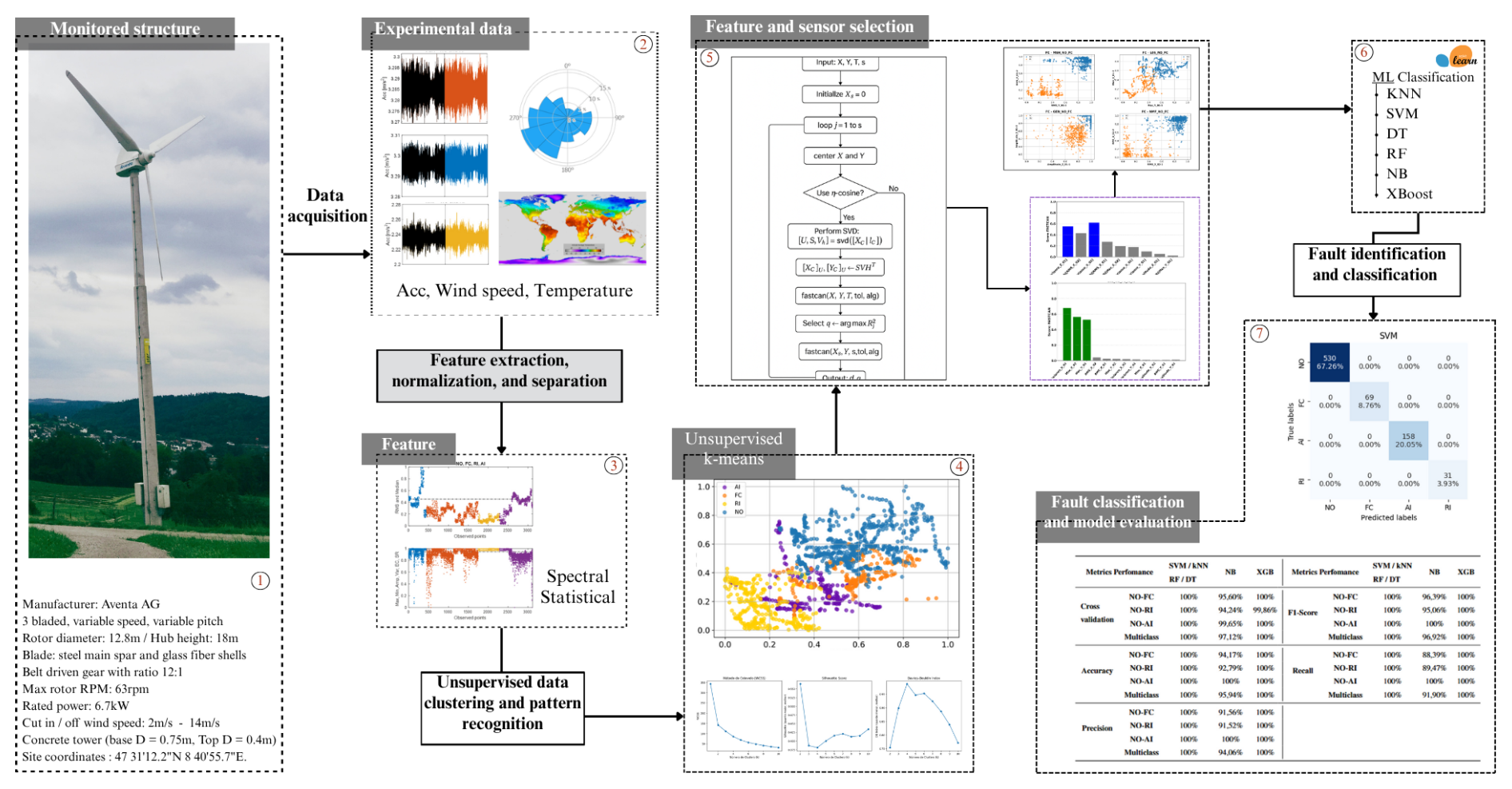
Figure 1 Pipeline of the hybrid machine learning model for fault classification on the Aventa 6.7 kW wind turbine.

2.1 Data processing, signal, and sensor analysis

The wind turbine monitored in this study is the Aventa AV-7 model, manufactured by Aventa AG (Switzerland) and commissioned by ETH. This turbine has a rated power of 6.7 kW and operates using a belt-driven generator coupled with a frequency converter and a variable-speed drive. It begins generating power at a wind speed of 2 m s⁻¹ and has a cut-off speed of 14 m s⁻¹. The rotor has a diameter of 12.8 m with three blades and is mounted at a hub height of 18 m. The maximum rotational speed reaches 63 rpm. Turbine control is managed through a variable-speed and variable-pitch mechanism. The turbine is installed in Taggenberg, Switzerland (coordinates: 47°31^′12.2^′′ N, 8°40^′55.7^′′ E). Instrumentation and data acquisition were provided in Chatzi et al. (2023) and include 14 accelerometers strategically placed along the tower, on the nacelle main frame, the main bearing, and the generator, as shown in Fig. 2. Additionally, two full-bridge strain gauges are mounted at the tower base to measure fore-aft and side-to-side strain, which can be converted into bending moments. Acceleration and strain signals are sampled at 200 Hz. Environmental measurements, including temperature and humidity, are collected at the tower base at a sampling rate of 1 Hz. Operational performance data (SCADA), including wind speed, nacelle yaw orientation, rotor RPM, power output, and turbine status, are recorded at 10 Hz. To ensure data quality and enhance the reliability of fault detection, a comprehensive supervised data preprocessing was implemented. This included supervised sensor analysis, outlier removal, signal segmentation, detrending, feature extraction, normalization, and similar feature identification and grouping.

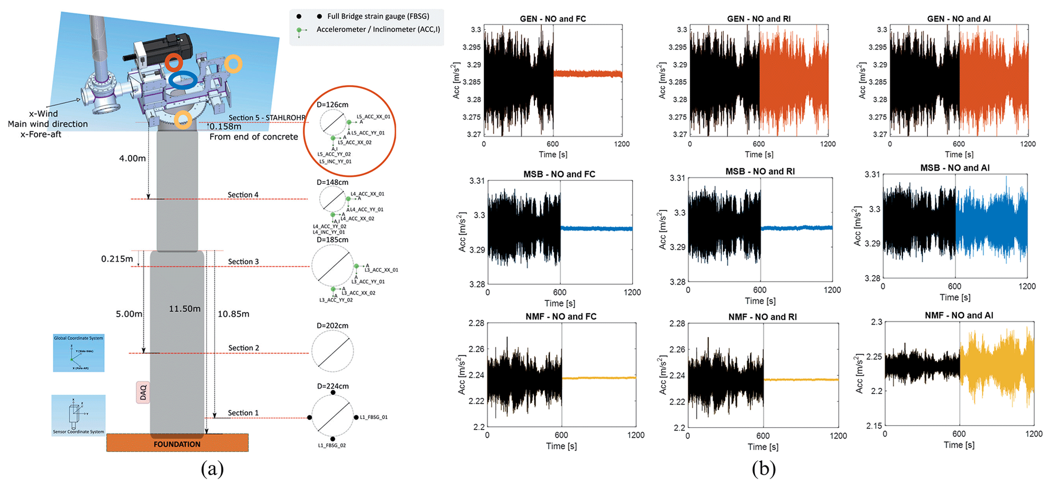
Figure 2 Schematic representation of the turbine sensor channel and location (Chatzi et al., 2023). SCADA data and accelerometers marked in orange, blue, and yellow colours are adopted in the monitoring (a). Temporal signal data of the turbine's NO and operation with failures (b): top: sensor GEN NO-FC, NO-RI, and NO-AI placed from left to right, respectively; middle: sensor MSB NO-FC, NO-RI, and NO-AI; and bottom: sensor NMF NO-FC, NO-RI, and NO-AI.

Table 1 Information on SCADA data and accelerometers used in the monitoring, with the respective sensor channel and location.

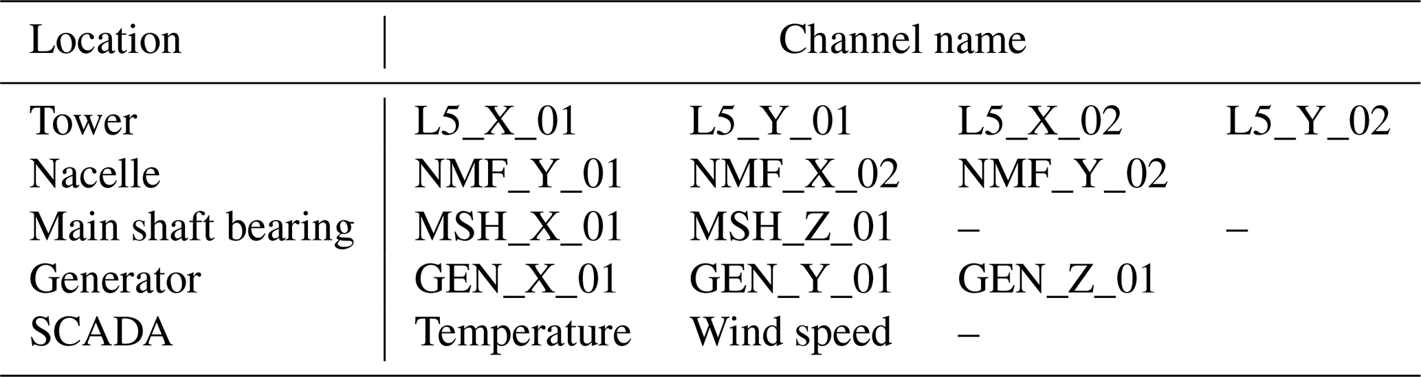
The data preprocessing stage begins by analysing the sensors' physics and evaluating each sensor's contribution to failure identification. The pre-established failures are the rotor icing event (RI), the flexible coupling of the linear drive of the collective pitch system (FC), and aerodynamic imbalance on one blade (AI). The Aventa dataset provides three-axis acceleration signals. Table 1 lists the SCADA data and accelerometers used for monitoring, along with their respective sensor channels and locations. The x axis captures side-to-side turbine motion, and the y axis captures fore-aft turbine motion. Figure 2a illustrates the sensor locations within the turbine. Aside from the SCADA data (temperature and wind velocity), accelerometers marked in orange, blue, and yellow are used for monitoring. Specifically, three accelerometers are located in the nacelle, GEN_ACC (orange), NMF_ACC (blue), and MSB_ACC (yellow); and one is located at the tower top, F5_ACC. The sensors record signals under the different operational conditions, including normal operation (NO). Figure 2 also presents the raw temporal data available in the dataset. In the acceleration graphs, black lines indicate normal turbine operation, whereas coloured lines represent various failure conditions. To ensure consistent comparisons, all signals were selected from the same day, minimizing the influence of changing environmental conditions.

The top row of graphs shows the x axis response from the generator-mounted sensor (GEN), comparing NO with failures FC, RI, and AI, from left to right. The middle row displays the x axis response from the main shaft bearing sensor (MSB), and the bottom row shows the same for the nacelle main frame sensor (NMF), following the same failure comparison pattern. Both x and y axis signals were analysed, revealing consistent trends: FC failures led to a pronounced amplitude reduction, whereas RI and AI failures resulted in only minor amplitude changes. These variations may fluctuate daily due to environmental conditions. To ensure effective fault detection, data from accelerometer sensors placed at the tower top, nacelle, main shaft bearing, and generator were used in the model, considering their sensitivity to structural, mechanical, and aerodynamic failures.

2.2 Dataset

During data analysis, duplicate files were identified, prompting a data redistribution strategy to eliminate redundancies and streamline the process. The data were categorized and colour-coded by operational conditions and events, making patterns – such as seasonality, frequency, and duration – more apparent and visually accessible. These cleaning and reorganization steps ensure that the same data are not reused across different turbine operations, thereby reducing the risk of misclassification and misinterpretation during monitoring.

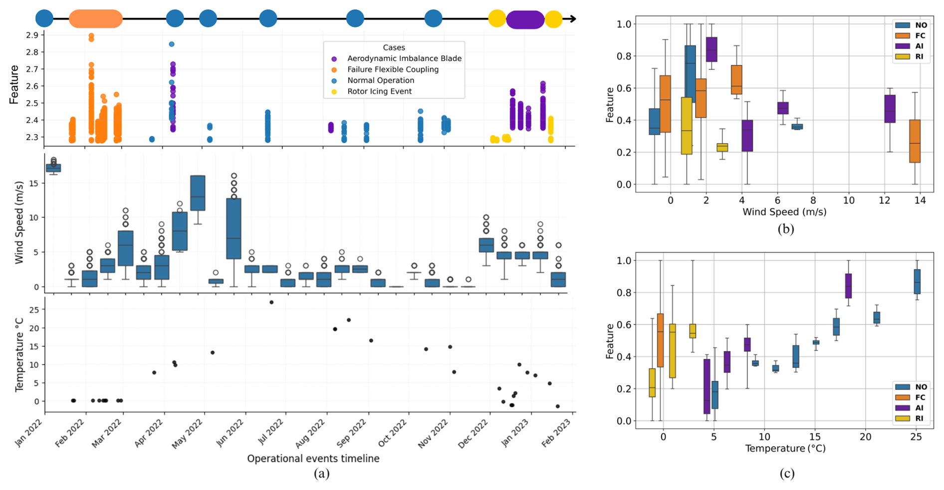
Figure 3 The feature dataset volume over the monitoring timeline categorized by yellow indicates RI, blue denotes NO, purple corresponds to AI, and orange represents the FC condition (a) (top). Wind speed boxplot (a) (middle), and mean temperature ((a) bottom). Boxplot of L05 sensor feature by wind speed variation (b) and feature by temperature variation (c).

Feature extraction was performed after this reorganization. Aside from the accelerometer sensors, the supervisory control and data acquisition (SCADA) data include the temperature, wind speed, humidity, and power output. Temperature, wind speed, and acceleration responses are used for monitoring. Figure 3a shows the maximum values of the temporal spectrum for each operational condition mapped over the monitoring timeline. Each condition is colour-coded for clarity: yellow for RI, blue for NO, purple for AI, and orange for flexible FC. Events are plotted along the horizontal axis to highlight their temporal distribution. The timeline begins with a NO sample, followed by a pitch drive coupling failure recorded on 16 February 2022, which required replacement. From April to November 2022, the turbine operated normally, during which AI was intentionally simulated using roughness tape on the blades. Additionally, naturally occurring RI events were observed between December 2022 and February 2023. Wind speed fluctuates throughout the monitoring period, as indicated by the boxplot, which displays the minimum, maximum, median, and first and third quartiles of the wind speed data. Meanwhile, ambient temperature ranges from −2 to 26 °C throughout the year (see Fig. 3c).

Both environmental conditions – wind speed and temperature – significantly influence the dynamic response of the wind turbine over time. Figure 3b–c present boxplots showing the feature values corrected by wind speed and temperature, respectively. This analysis focuses on the RMS value of sensor NMF, selected for its highest-scoring features and well-defined failure patterns, which represent the general behaviour of the features. When correlating feature values with wind speed, the FC and AI conditions exhibit the greatest sensitivity to increasing wind speeds, though with relatively low dispersion. Conversely, RI, NO, and FC show higher maximum, minimum, and quartile values at lower wind speeds. Regarding temperature, rising temperatures primarily affect NO and AI conditions, whereas lower temperatures have a greater impact on FC and RI. These findings underscore the importance of incorporating environmental variables into the monitoring framework to improve the robustness and accuracy of fault classification. The SCADA data in the general dataset are considered the mean temperature and mean wind speed, both acquired over the 24 h of the respective day.

2.3 Feature extraction, normalization, and dataset organization

Feature selection involves choosing a subset of variables from the original dataset. This step transforms the spectrum data into new variables to create a refined dataset (Bishop, 2006). Fifteen features are formulated using the time-domain signal (Knittel et al., 2019; Barreto et al., 2021; Ashkarkalaei et al., 2025a), as presented in Table 2, where x is the temporal spectrum signal and p is the sampling points value.

Table 2 Temporal and statistical formulation used for feature extraction.

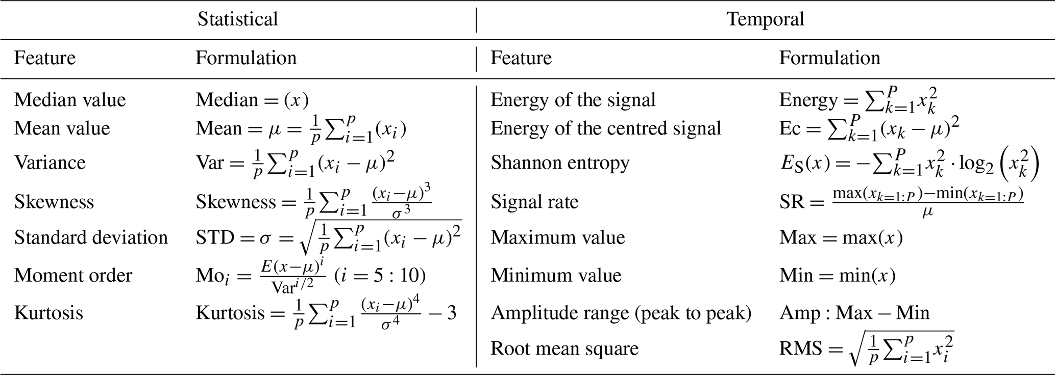
Temporal features are extracted from a signal's frequency or time content, such as maximum, minimum, amplitude range, energy, energy centre, skewness, signal rate, and RMS. It captures how the signal's energy is distributed over time. Statistical features, in turn, are computed from the signal's time-domain values, including the median, mean, variance, skewness, kurtosis, higher-order moments, and standard deviation, which characterize the overall distribution and variability of the signal. Together, these features are compiled, analysed, and evaluated for their similarity and sensitivity to the system's dynamic behaviour.

Despite feature refinement and grouping, the remaining features still pose a challenge due to their minimal amplitude variation, often differing by only a few digits. Such small variations can hinder accurate machine learning classification. To address this issue, the proposed relative change damage index incorporates a normalization step based on the relative change of each feature, defined as

$$\begin{array}{}\text{(1a)}& {\displaystyle }{\mathrm{\Delta }}_{\mathrm{f}}& {\displaystyle }=max\left({\mathbf{X}}_i\right)-{\mathbf{X}}_i\text{(1b)}& {\displaystyle }\text{RC}& {\displaystyle }={\displaystyle \frac{{\mathrm{\Delta }}_f}{max\left({\mathrm{\Delta }}_f\right)}},\end{array}$$

where X is a table containing the selected features and Δ_f measures each feature's deviation from its maximum value within the selected feature set to each feature vector point (X_i). The normalization factor RC rescales these deviations to the [0, 1] interval. This linear transformation preserves the original ordering and proportionality of the data, ensuring that the intrinsic dynamic pattern is maintained. At the same time, it amplifies subtle differences that would otherwise be masked by small numerical variations, thereby enhancing the sensitivity of the features for fault detection and classification. Hence, the RC normalization converts the data into dimensionless features that, prior to normalization, differed only slightly (e.g. 3.280 vs 3.286), rendering these differences numerically negligible for machine learning models. Thus, the proposed approach amplifies these small variations while preserving the intrinsic dynamic pattern. Features with values close to unity correspond to undamaged conditions, whereas values approaching zero indicate faults. Hence, the method enhances fault sensitivity and enables consistent comparison across features of different magnitudes, making the damage feature more sensitive to anomalies under varying operating states.

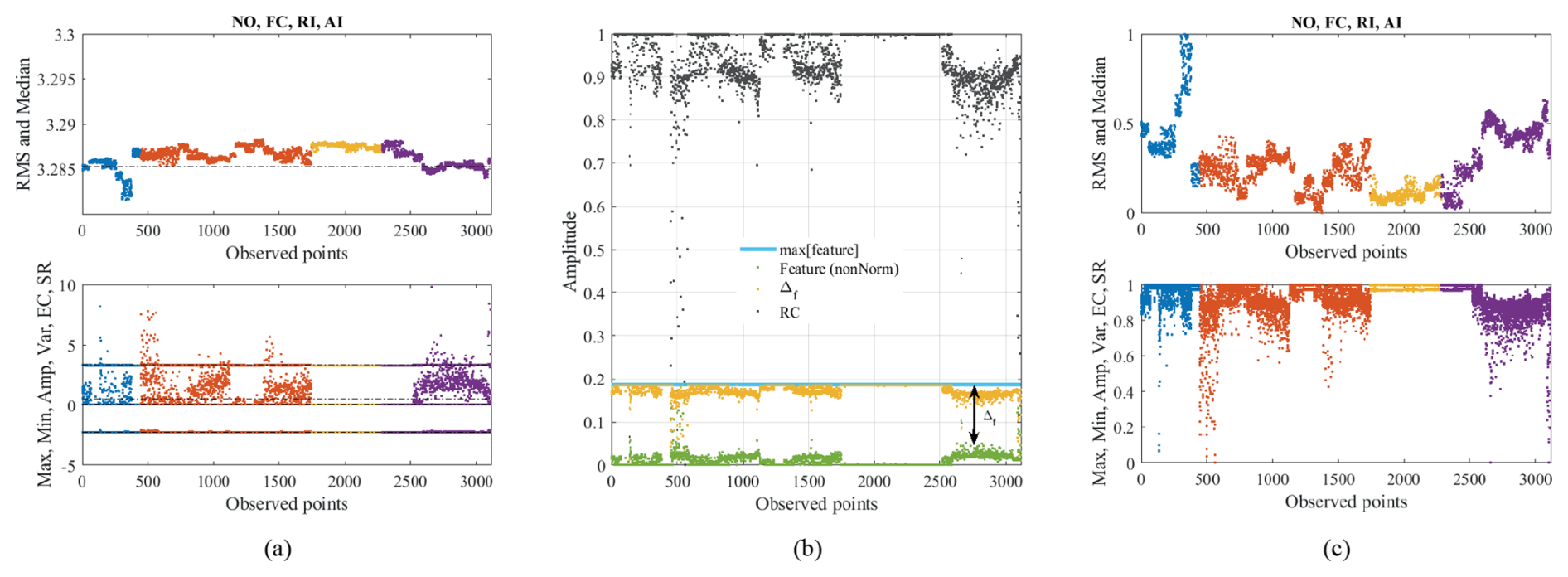
Figure 4 (a) Non-normalized features grouped by similarity under different operating conditions: NO – blue, FC – orange, RI – yellow, and AI – purple. (b) Demonstration of the scaling and normalization on the Amp feature related to Eq. (1). Scaled and normalized features grouped by similarity under different conditions (c).

The relative change normalization provides a theoretical foundation based on relative scaling and dimensionless feature representation. Figure 4a–c illustrates the process: (a) the non-normalized features, (b) the scaling and normalization applied to the Amp feature (extended to all others), and (c) the normalized features obtained using the proposed relative change technique. Features such as energy, kurtosis, higher-order moments, and Shannon entropy exhibited low sensitivity to failures and were excluded during normalization and analysis. This first supervised analysis revealed two feature groups with similar behaviour. Group 1 consists of the RMS and median (Fig. 4c, top), while Group 2 comprises the maximum, minimum, amplitude range, variance, energy centre, and signal rate (Fig. 4c, bottom). The formation of two feature groups indicates a high degree of correlation within each group, with RMS and median primarily capturing the signal's central tendency. In contrast, the features of Group 2 describe its variability and extremes. Therefore, using all features would introduce redundancy, increase computational cost, and risk overfitting due to the curse of dimensionality. Selecting only representative features from each group ensures that the classifier retains the essential discriminatory information while improving efficiency and generalization.

From the two correlated feature groups, four representative features (RMS, maximum, variance, and amplitude range) were selected to compose the global dataset. Those four features were chosen over the other in their respective group due to near-equivalence, thus avoiding redundancy. The initial global dataset, therefore, consisted of the four selected features extracted from each sensor axis, resulting in a structure of measurement_rows × 48 columns, plus the SCADA data, as detailed in Table 1. However, including all these features may appear arbitrary and degrade model performance due to their high similarity. To refine the global dataset, a canonical correlation analysis was applied to identify the most sensitive features for each sensor, accounting for all axes simultaneously within the sensor group. The highest feature correlation scores were selected, reducing the dataset to four representative features plus SCADA. This process yielded the final datasets: the binary classification dataset has six columns (four features plus SCADA), and the multi-class dataset has nine columns (selected features plus SCADA). Identifying the most informative sensor is also relevant, as it indicates which sensor contributes most to classification accuracy and provides resilience in the event of sensor loss. To validate this study, the most sensitive feature from the best-performing sensor was removed in subsequent tests, thereby demonstrating the robustness and consistency of the proposed feature selection strategy. Feature and sensor selection are detailed in Sect. 2.1.

Structured final datasets

The final refined dataset organization is a crucial step for enabling machine learning algorithms to accurately classify operational failures. The deployed dataset exhibits a multimodal nature, integrating structural, temperature, and wind velocity information. The structural data are directly acquired from the accelerometers, which capture the system's physical response and potential failure signatures. In contrast, temperature and wind speed data are obtained from the SCADA system and represent indirect but relevant variables that influence the dynamic behaviour measured by the accelerometers. However, they do not directly describe the damage dynamics. The final dataset is organized into four configurations, which are evaluated. Their relevance is demonstrated in Sect. 4, yielding the following:

• Fe-kms-Sc. Dataset composed of the selected features (Fe) extracted from the accelerometer time signals, followed by the SCADA data (Sc) and label defined by the k-means clustering (kms),

• Fe-Sc-kms. Dataset including the selected features, the SCADA data, and the corresponding k-means labels,

• Fe-kms. Dataset including the selected features and the k-means labels, without incorporating the SCADA information,

• Fe-kms-LoseSensor. Dataset including the selected features excluding those obtained from the most sensitive sensor identified by the Fast CCA method, together with the k-means labels and SCADA data. This configuration simulates the loss of the most sensitive sensor in each analysis scenario.

The k-means labelling of the datasets Fe-kms-Sc and Fe-kms-LoseSensor is applied exclusively to the features that contain the most relevant physical information about the damage. The SCADA data are then organized by the corresponding day and hour for each feature sample. This ensures that the SCADA records follow the same row reordering imposed by the k-means clustering, while preserving the correct temporal (day and hour) correspondence between the SCADA measurements and the related accelerometer data.

3 Hybrid machine learning model

The monitoring model integrates sequential stages, starting with data processing and feature extraction, followed by pattern recognition through clustering, and extending to feature and sensor selection to strengthen dataset reliability. By coupling unsupervised clustering with canonical-correlation-based feature selection, the framework ensures the preservation of the most informative variables, thereby enhancing classification accuracy.

3.1 Pattern recognition and clustering

Unsupervised pattern recognition, labelling, and clustering of the normalized features were performed using the k-means algorithm, with the elbow method applied to determine the optimal number of clusters. The silhouette coefficient and Davies–Bouldin index are internal validation metrics used to assess the number and quality of clusters identified by k-means. Table 3 lists the k-means metrics for each sensor and case of study.

Table 3 k-means clustering identification for each sensor related to the failure associated with the silhouette coefficient and Davies–Bouldin index performance metrics.

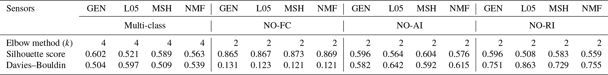
For binary cases (k=2), the results indicate good separability between operating conditions, with consistent metrics across different components and failure types. In NO-FC scenarios, silhouette score values remain high (between 0.86 and 0.87), and Davies–Bouldin indices are low (between 0.12 and 0.13), indicating that points within each group are very similar to each other and that the clusters are well separated. In NO-RI and NO-AI conditions, the results still exhibit a satisfactory clustering structure, with silhouette values ranging from 0.56 to 0.60, and Davies–Bouldin scores between 0.58 and 0.75, indicating good cluster quality. In general, all binary-scenario cases yielded metrics superior to the reference values recommended in the literature (silhouette >0.5 and Davies–Bouldin <1.0), confirming that the clustering method can adequately distinguish the different operational states of the turbines. For the multi-class case with k=4, the validation metrics indicate good clustering quality. Silhouette score values range from 0.52 to 0.60, and the Davies–Bouldin index values range from 0.50 to 0.60, indicating compact and well-separated clusters. These results confirm that the clustering process identified variations in turbine operational states. Therefore, these metrics provide strong evidence that the clustering step is reliable and that the labels assigned during the unsupervised phase are consistent.

Table 4 Explicit description of the datasets used for training, validation, and testing.

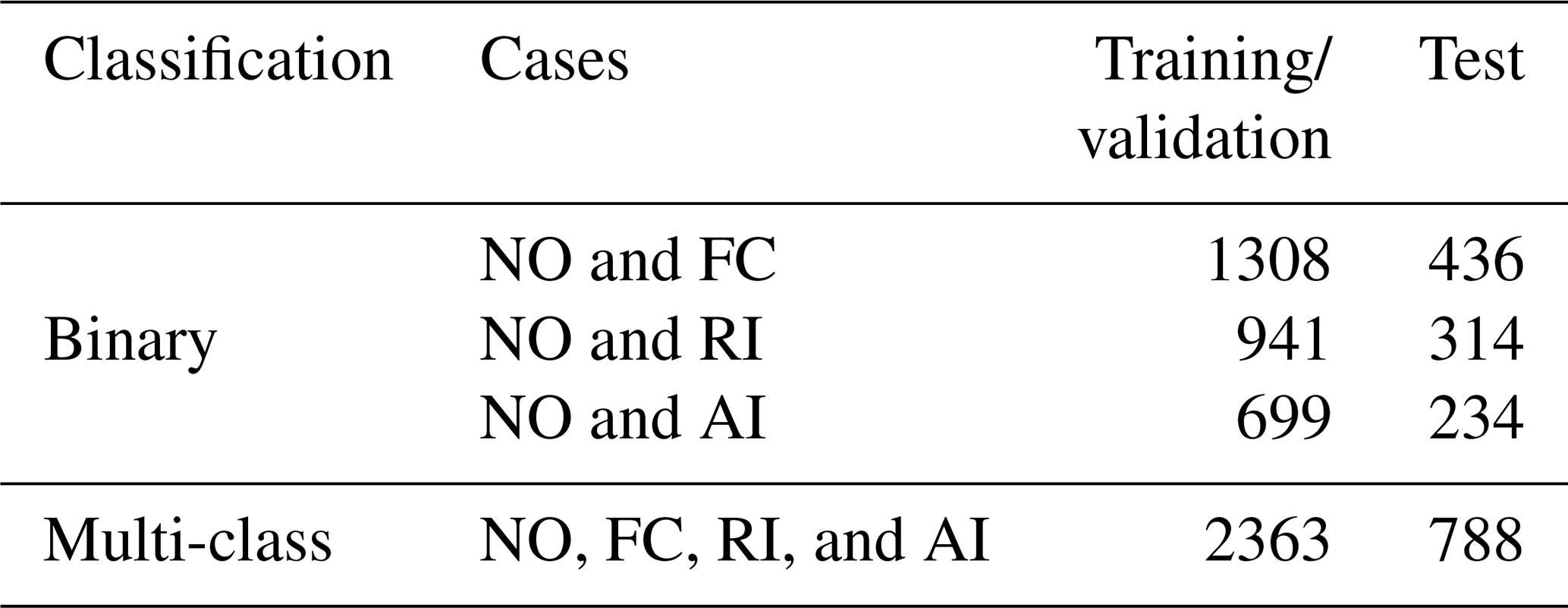
The outputs are subsequently used as inputs for the feature and sensor selection. Furthermore, the samples were randomly divided, and the clustered dataset was split into training/validation 75 % and test 25 %, which were used for model construction and evaluation, as shown in Table 4. Each classifier was assessed using a 5-fold cross-validation procedure to enhance training accuracy, which was achieved by randomly partitioning the training dataset into five distinct subsets.

3.2 Feature and sensor fast selection

The supervised feature analysis indicates that changes in the turbine's dynamic behaviour are associated with specific events. For the subsequent procedures, feature and sensor selection are performed using the canonical-correlation-based feature selection method (FASTCAN) introduced by Zhang et al. (2025), which was initially applied only for feature selection and is extended in this work to include sensor selection. Therefore, the selection process is carried out in two steps: first, identifying the best feature(s) for each sensor and, second, selecting the most relevant sensor(s). The pseudocode for this process is given in Algorithm 2, which is repeated for each fault diagnosis. The FASTCAN method is based on the canonical correlation coefficient (CCA), a measure of the linear association between two multivariate random variables. It evaluates the relevance of features with respect to the response matrix. Given the feature matrix $\mathbf{X}\in {\mathbb{R}}^{N\times n}$ and the response matrix $\mathbf{Y}\in {\mathbb{R}}^{N\times m}$, the canonical correlation coefficient is defined as

$$\begin{array}{}\text{(2)}& R_i(\mathbf{X},\mathbf{Y})=\underset{{\mathit{\alpha }}_i,{\mathit{\beta }}_i}{max}r({\mathbf{X}}_{\mathrm{C}}{\mathit{\alpha }}_i,{\mathbf{Y}}_{\mathrm{C}}{\mathit{\beta }}_i),\end{array}$$

where X_C and Y_C are column-centred matrices and $r(\cdot ,\cdot )$ denotes the Pearson correlation. The projection vectors α_i∈ℝⁿ and β_i∈ℝ^m are obtained by solving the following eigenvalue problems:

$$\begin{array}{}\text{(3)}& {\displaystyle }\left({\mathbf{X}}_{\mathrm{C}}^{\top }{\mathbf{X}}_{\mathrm{C}}{)}^{-\mathrm{1}}{\mathbf{X}}_{\mathrm{C}}^{\top }{\mathbf{Y}}_{\mathrm{C}}\right({\mathbf{Y}}_{\mathrm{C}}^{\top }{\mathbf{Y}}_{\mathrm{C}}{)}^{-\mathrm{1}}{\mathbf{Y}}_{\mathrm{C}}^{\top }{\mathbf{X}}_{\mathrm{C}}{\mathit{\alpha }}_i& {\displaystyle }=R_i^{\mathrm{2}}(\mathbf{X},\mathbf{Y}){\mathit{\alpha }}_i\text{(4)}& {\displaystyle }\left({\mathbf{Y}}_{\mathrm{C}}^{\top }{\mathbf{Y}}_{\mathrm{C}}{)}^{-\mathrm{1}}{\mathbf{Y}}_{\mathrm{C}}^{\top }{\mathbf{X}}_{\mathrm{C}}\right({\mathbf{X}}_{\mathrm{C}}^{\top }{\mathbf{X}}_{\mathrm{C}}{)}^{-\mathrm{1}}{\mathbf{X}}_{\mathrm{C}}^{\top }{\mathbf{Y}}_{\mathrm{C}}{\mathit{\beta }}_i& {\displaystyle }=R_i^{\mathrm{2}}(\mathbf{X},\mathbf{Y}){\mathit{\beta }}_i.\end{array}$$

The eigenvalues $R_i^{\mathrm{2}}(\mathbf{X},\mathbf{Y})$ correspond to the squared canonical correlation coefficients, while α_i and β_i are the canonical weight vectors that define the canonical variates X_Cα_i and Y_Cβ_i. There are at most $min(n,m)$ non-zero canonical correlation coefficients $R_{\mathrm{1}}(\mathbf{X},\mathbf{Y}),\mathrm{\dots },R_{min(n,m)}(\mathbf{X},\mathbf{Y})$. The overall criterion for feature selection is the sum of squared canonical correlations (SSC):

$$\begin{array}{}\text{(5)}& \text{SSC}(\mathbf{X},\mathbf{Y})=\sum _{k=\mathrm{1}}^{min(n,m)}{R}_k^{\mathrm{2}}(\mathbf{X},\mathbf{Y}).\end{array}$$

To accelerate computation, the SSC can be reformulated using two equivalent decompositions: (i) the h-correlation form (valid when $N\le n+m$),

$$\begin{array}{}\text{(6)}& \text{SSC}(\mathbf{X},\mathbf{Y})=\sum _{i=\mathrm{1}}^n\sum _{j=\mathrm{1}}^m{r}^{\mathrm{2}}(w_i,v_j),\end{array}$$

where {w_i} and {v_j} are orthogonal bases of the feature and response spaces; and (ii) the θ-angle form (valid when $N>n+m$),

$$\begin{array}{}\text{(7)}& \text{SSC}(\mathbf{X},\mathbf{Y})=\sum _{i=\mathrm{1}}^n\sum _{j=\mathrm{1}}^m{\cos }^{\mathrm{2}}\left(\mathrm{\angle }\right(w_i,v_j\left)\right),\end{array}$$

where the canonical correlations are expressed as squared cosines of the principal angles between the subspaces of X and Y. In the greedy selection step, the next feature x_ri is chosen to maximize the incremental SSC:

$$\begin{array}{}\text{(8)}& d=\arg \underset{i}{max}\sum _{k=\mathrm{1}}^{min(p+\mathrm{1},m)}{R}_k^{\mathrm{2}}\left(\right({\mathbf{X}}_{\mathrm{s}},x_{ri}),\mathbf{Y}),\end{array}$$

where X_s denotes the already selected features. This formulation allows efficient feature ranking by reducing computational complexity while preserving the theoretical properties of canonical correlation analysis.

This process involves looping through the features for each sensor in an interaction. In sequence, a similar procedure is performed for sensor ranking, with the feature matrix defined as ${\mathbf{X}}_{\mathrm{s}}\in {\mathbb{R}}^{S\times s}$, where X_s contains the highest ranking feature(s) of each sensor.

Algorithm 2 Pseudocode for the feature and sensor selection with canonical correlation.

Input: $\mathbf{X}\in {\mathbb{R}}^{N\times n}$ Candidate feature matrix

Input: $\mathbf{Y}\in {\mathbb{R}}^{N\times m}$ Target multi-label matrix

Output: $\mathbf{d}\in {\mathbb{R}}^{\mathrm{1}\times \mathcal{T}}$, where $\mathbf{d}=(d_{\mathrm{1}},d_{\mathrm{2}},\mathrm{\dots },d_t)$ Index of the feature with the highest ranking score

Output: $\mathbf{q}\in {\mathbb{R}}^{\mathrm{1}\times s}$, where $\mathbf{q}=(q_{\mathrm{1}},q_{\mathrm{2}},\mathrm{\dots },q_{\mathrm{s}})$ Index of the feature with the highest ranking score associated with the sensor

1:

𝒯∈N Number of features to be selected

2:

s∈S Number of sensors

3:

X_s←0 Candidate feature matrix coating the best feature(s) of each sensor. The threshold score is ≥0.6

4:

for j←1 to s do

5:

${\mathbf{X}}_{\mathrm{C}}\leftarrow [\mathbf{X}-\text{mean}(\mathbf{X})$], ${\mathbf{Y}}_{\mathrm{C}}\leftarrow [\mathbf{Y}-\text{mean}(\mathbf{Y}\left)\right]$

6:

if use η-cosine then

7:

$[\mathbf{U},\mathbf{S},{\mathbf{V}}_h^{\top }]\leftarrow \text{svd}\left(\right[{\mathbf{X}}_{\mathrm{C}}\mid {\mathbf{Y}}_{\mathrm{C}}\left]\right)$

8:

$[{\mathbf{X}}_{\mathrm{C}}{]}_U\mid [{\mathbf{Y}}_{\mathrm{C}}{]}_U\leftarrow {\mathbf{SV}}_h^{\top }$

9:

end if

10:

$R_i^{\mathrm{2}}\leftarrow \mathrm{0}$ for $i=\mathrm{1},\mathrm{\dots },n$Feature ranking scores

11:

d_i←0 for $i=\mathrm{1},\mathrm{\dots },t$ Output indices vector, where t∈N is the number of features to be selected

12:

procedure FASTCAN X, Y, t, tol, alg Function described in Zhang et al. (2025)

13:

$d\leftarrow \arg {max}_j{R}_j^{\mathrm{2}}$

14:

return d

15:

${\mathbf{X}}_{\mathrm{s}}\leftarrow \mathbf{X}[:,max(\mathbf{d}\left)\right]$ Highest score feature

16:

end for

17:

procedure FASTCAN X_s, Y, s, tol, alg

18:

$\text{q}\leftarrow \arg {max}_j{R}_j^{\mathrm{2}}$

19:

return q

3.3 Classification and model evaluation

ML algorithms are applied to classify the operational condition of the wind turbine by analysing datasets. As an automated approach, ML identifies patterns in data through various algorithms, and uses these learned patterns for predictive analysis and decision-making. The proposed model follows a hybrid unsupervised-supervised ML-based framework, incorporating classification strategies to improve the structure of data attributes. The data-driven ML models are fed selected features extracted from the multiphysics database, incorporating vibration responses and environmental data, and the output corresponds to the wind turbine's operational classification state.

For the classification task, six supervised ML algorithms are utilized, and the unsupervised k-means algorithm is used for initial clustering. At the same time, the supervised classifiers Naive Bayes (NB), decision tree (DT), random forest (RF), kNN, SVM, and extreme gradient boosting (XGB) are employed to detect the system's operational conditions. The ML algorithms embedded in the framework are based on the open-source Scikit-learn library. These algorithms perform final classification based on the initial clustering results, producing outputs including confusion matrices and performance metrics. The selection of hyperparameters follows the recommendations in de Sousa et al. (2023) and Coelho et al. (2024, 2025), which identified optimal configurations for this application. Specifically, the SVM model employs a linear kernel with a penalty parameter of C=100, a one-vs-one multi-class strategy, and a tolerance of $\mathrm{1}\times {\mathrm{10}}^{-\mathrm{3}}$. For kNN, the number of neighbours is set to k=3, using the Euclidean distance metric, uniform weights, and a leaf size of 30. The RF and DT algorithms both use 100 trees, a maximum depth of 3, and the Gini splitting criterion. The Naive Bayes classifier employs a Gaussian model, while XGBoost uses the XGBClassifier implementation. These configurations have shown high accuracy and robustness in prior studies, and are adopted here to optimize classification performance.

The final step involves evaluating model performance on a previously separated test dataset. Hyperparameters may be fine-tuned to improve accuracy, precision, recall, and the F1-score. A confusion matrix is also analysed to provide further diagnostic insight. To prevent overfitting and ensure generalizability, a 5-fold cross-validation scheme is employed. Performance metrics and confusion matrices are generated for all algorithms, enabling the framework to identify the most accurate model and guide users in selecting the most suitable ML algorithm for wind turbine monitoring.

4 Results and discussion

During the monitoring process, data from various sensors are available. To ensure accurate failure identification and classification, it is essential to evaluate the most informative sensor data. In the proposed framework, both features and sensors are ranked and selected to compose the reduced dataset, ensuring that only the most sensitive information related to the specific failure is included and fed into the ML algorithm for wind turbine condition classification. The feature and sensor scores, normalized to the range [0, 1], are returned by the CCA's ranking process. Further, the dataset for the ML algorithms was built by selecting the top-ranked features from each sensor, along with the SCADA wind speed and temperature.

The evaluation of the turbine's operational condition includes both binary and multi-class classification tasks. Table 5 summarizes the failure cases related to the most sensitive feature of each sensor (X_s) and the most sensitive sensor associated with its features for each failure.

Table 5 Description of the sensitive feature of each sensor (X_s) and an indication of the most sensitive sensor of each failure case.

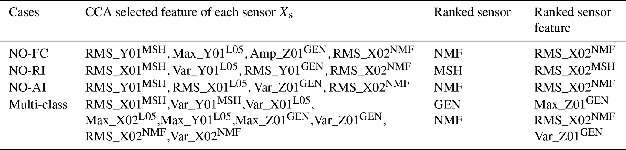
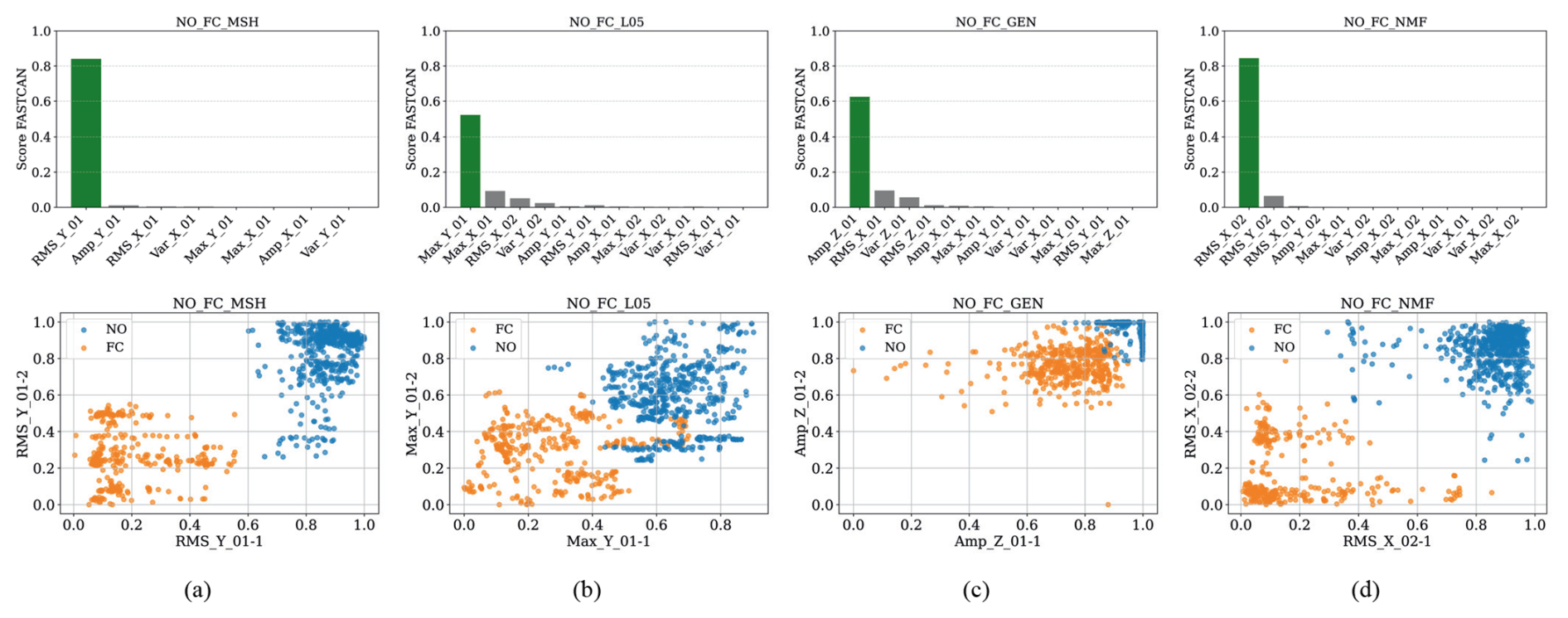
Figure 5 CCA feature score and dispersion diagrams of the highest-scoring feature for the NO-FC failure: (a) sensor MSH, (b) sensor L05 (1 and 2), (c) sensor GEN, and (d) sensor NMF (1 and 2).

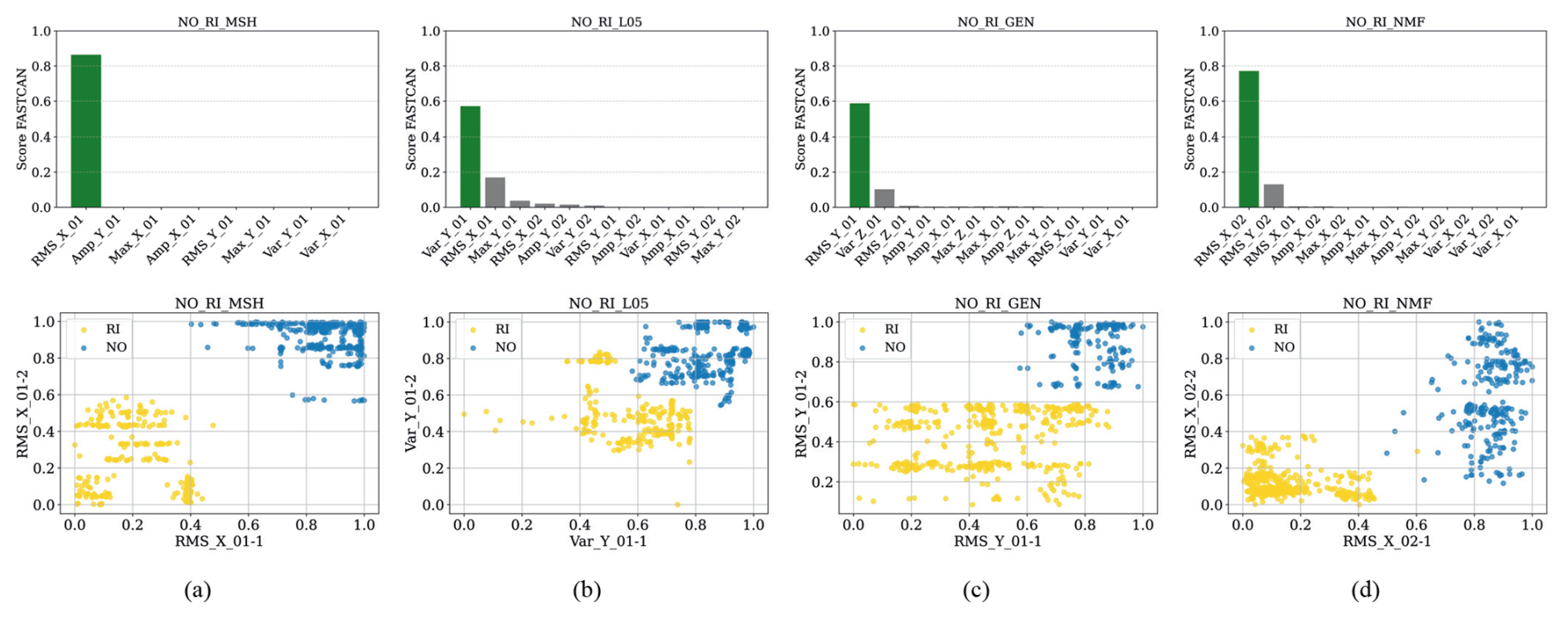
Figure 6 CCA feature score and dispersion diagrams of the highest-scoring feature for the NO-RI failure: (a) sensor MSH, (b) sensor L05 (1 and 2), (c) sensor GEN, and (d) sensor NMF (1 and 2).

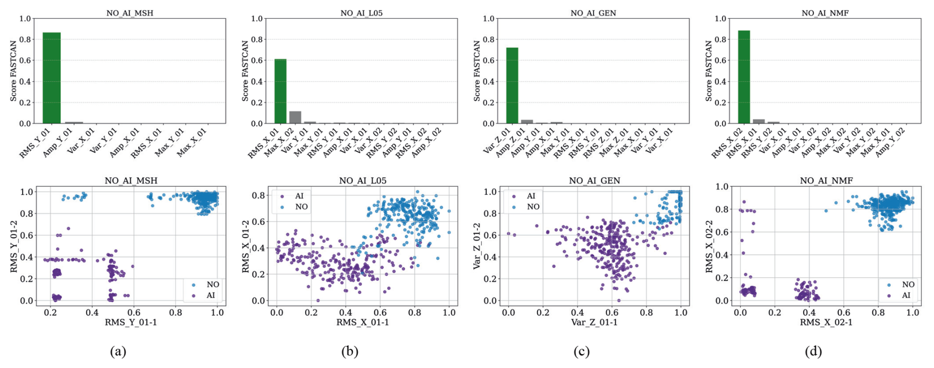
Figure 7 CCA feature score and dispersion diagrams of the highest-scoring feature for the NO-AI failure: (a) sensor MSH, (b) sensor L05 (1 and 2), (c) sensor GEN, and (d) sensor NMF (1 and 2).

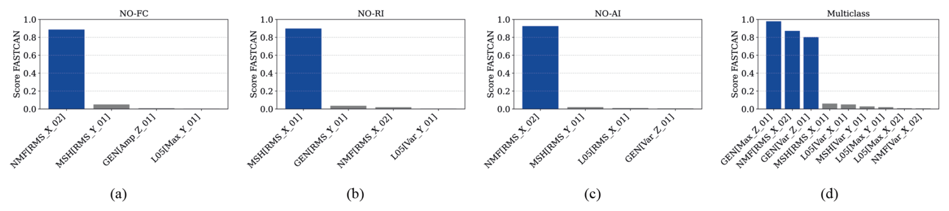
Figure 8 Sensor score based on the top-performing features of each operational condition: (a) NO-FC, (b) NO-AI, (c) NO-RI, and (d) multi-class.

For binary classification between NO and FC failure, the individual feature scores for each accelerometer sensor are shown in Fig. 5a–d. Subsequently, in the sensor ranking, the NMF sensor (RMS_X02^NMF) yields the highest score, indicating it as the most sensitive to FC-related failures, as shown in Fig. 8a. The k-means algorithm is applied to label and organize the data based on similarities among the selected features. Incorporating more informative features improves both pattern recognition and classification accuracy. Each feature is visualized individually for clarity, and the final classification integrates all selected features along with SCADA data to strengthen the overall decision-making process. Features with minimal overlap between operational states are especially valuable, as they contribute to clearer distinctions and improved ML performance in identifying fault conditions. Scatter plots in Fig. 5e–h display the correlation between Feature-1 and Feature-2, which represent two groups derived from splitting each selected feature column. These diagrams highlight how high-scoring features cluster across sensors, revealing patterns that differentiate between normal and faulty operating conditions. The identified clusters exhibit consistent grouping and dispersion, thereby enhancing the interpretability of each operational condition.

For classification between NO and RI, the feature scores for each accelerometer are shown in Fig. 6a–d and Table 5, with the MSH sensor (RMS_X02^MSH) achieving the highest score, indicating strong sensitivity to RI-related anomalies, as indicated in Fig. 8b. The k-means clustering is applied to the selected features to identify patterns and assign labels. Scatter plots in Fig. 6e–h display the highest-scoring feature pairs (Feature-1 vs Feature-2) per sensor, revealing clear cluster separation between NO and RI. These dispersion diagrams highlight how specific failures impact dynamic behaviour, with minimal overlap between classes indicating highly informative features for classification. For the NO-AI, the feature ranking scores of each accelerometer are presented in Fig. 7a–d, where the NMF sensor (RMS_X02^NMF) shows the highest relevance, indicating strong responsiveness to RI-related conditions – see Fig. 8c. The k-means clustering is applied to the selected features to identify patterns and assign labels. The resulting scatter plots in Fig. 7e–h show the top-ranked feature pairs (Feature-1 vs Feature-2) for each sensor, revealing distinct cluster boundaries between NO and AI. These diagrams illustrate how different faults affect the turbine's dynamic behaviour, with low class overlap indicating that the selected features are highly effective for classification.

In the multi-class classification, the k-means algorithm identifies four clusters corresponding to NO, FC, RI, and AI conditions, organizing the dataset accordingly into response clusters. These clusters support further validation of classification through performance metrics. Figure 9 displays the highest-scoring features of each sensor and their related dispersion diagrams, labelled by k-means and ranked by Algorithm 2, respectively. Each class is colour-coded to facilitate quick visual identification and analysis of overlaps between operational states.

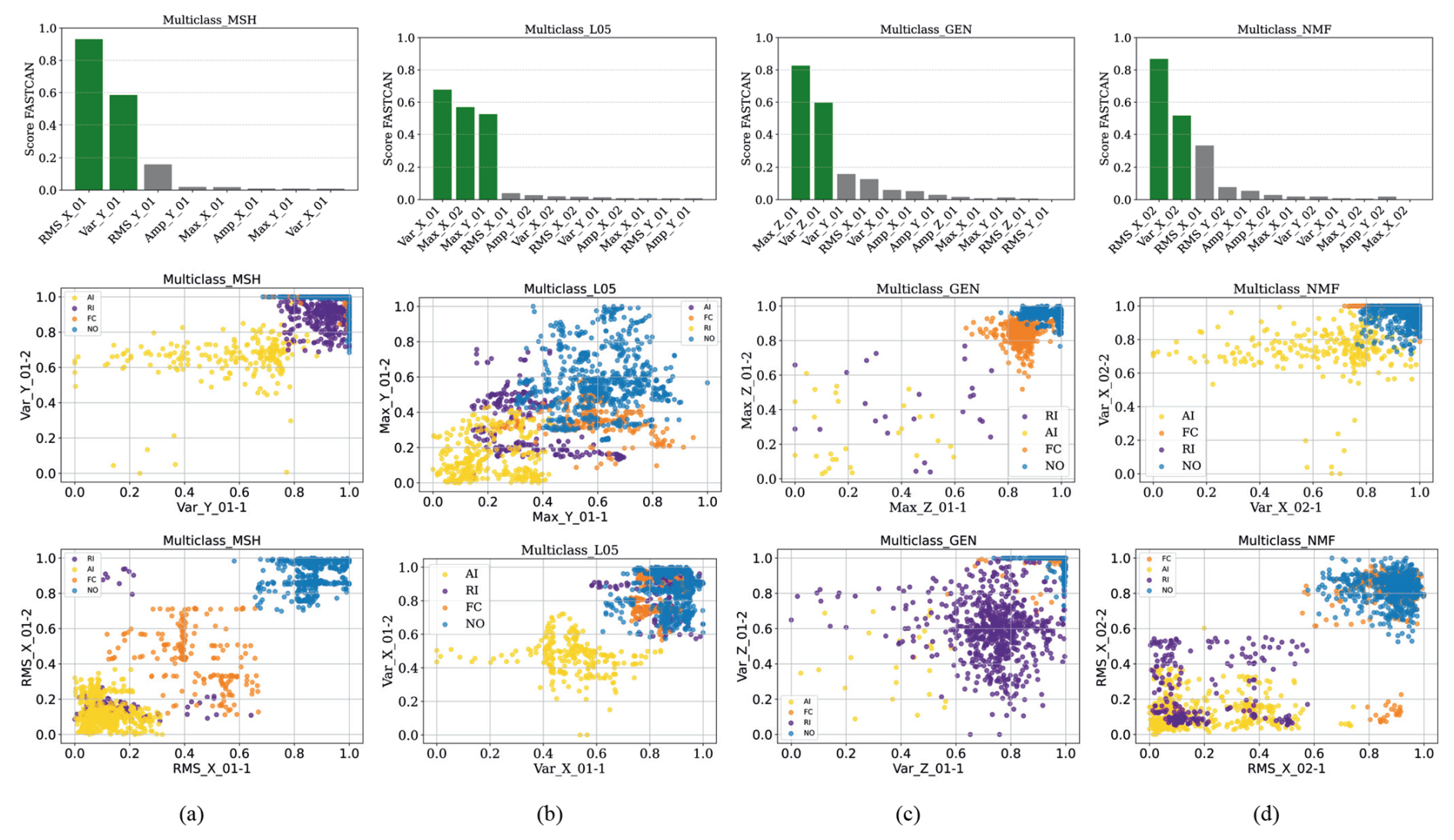
Figure 9 CCA feature score and dispersion diagrams of the highest-scoring feature: (a) sensor MSH, (b) sensor L05 (1 and 2), (c) sensor GEN, and (d) sensor NMF (1 and 2).

Figure 9a–d gives the top-ranked features from each sensor, MSH, L05, NMF, and GEN, respectively, highlighting the most sensitive sensors selected for multi-class classification. Likewise, in the binary case, features with higher scores are included in the global dataset for classification, with the GEN and NMF sensors showing the highest relevance, indicating strong sensitivity, as shown in Fig. 8d. Each selected feature is visualized through its dispersion correlation, also in Fig. 9a–d. Overall, k-means effectively assigns each operational fault to a class. Certain features exhibit a clear separation between normal conditions and fault types, although overlap among fault classes is evident in all cases. This suggests that while individual features may help to detect abnormal behaviour, they are not self-sufficient alone to discriminate between specific failure modes. These individual feature analyses reveal important patterns. However, when classification models are applied, features are considered in combination. This integrated approach improves both classification accuracy and the robustness of the performance metrics. While some features aid in distinguishing normal from faulty states, reliable fault classification generally requires the combined contribution of multiple informative features.

Operational condition classification and metrics evaluation

The fault classification uses six supervised machine learning algorithms: kNN, SVM, DT, RF, Naive Bayes, and XGBoost. These algorithms perform the final classification using the input dataset, producing confusion matrices and performance metrics. The selection of hyperparameters is based on the investigations of de Sousa et al. (2023), which specify optimal configurations for this assignment and are briefly described in Sect. 3.3.

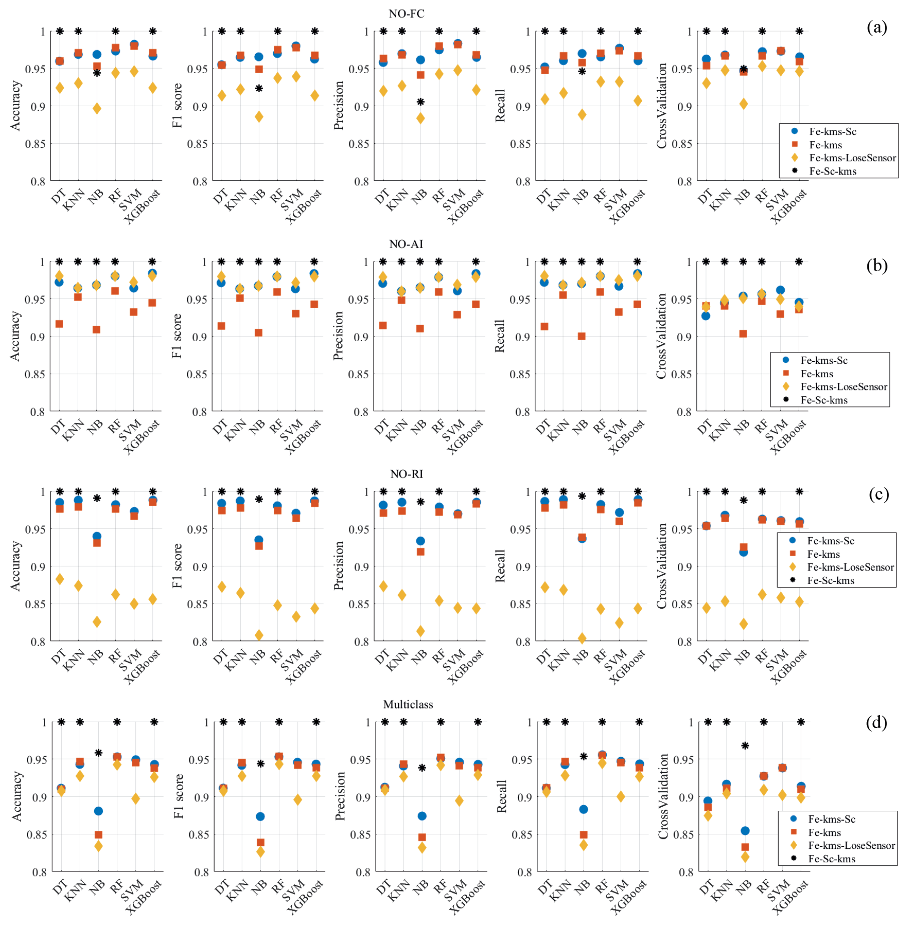
Figure 10 Comparison of the metrics (accuracy, F1-score, precision, recall, and cross-validation) for the six ML algorithms and each arranged final dataset. (a) Binary NO-FC, (b) binary NO-AI, (c) binary NO-RI, and (d) multi-class failure study cases.

Figure 10 presents the performance of ML models for binary classification (NO-FC, NO-RI, and NO-AI) and multiple failure conditions, evaluated via cross-validation and metrics such as accuracy, precision, recall, and F1-score. For metric estimation, micro-, macro-, and weighted averages were tested, assuming the micro as the standard because it computes classification metrics by globally summing true positives, false positives, and false negatives across all classes, resulting in similar precision, recall, and F1-score.

The ML models were tested on the Fe-kms-Sc, Fe-Sc-kms, Fe-kms, and Fe-kms-LoseSensor datasets to assess the influence of environmental dependencies (SCADA data) and the sensitivity of each sensor in failure evaluation. The metrics for the Fe-Sc-kms dataset, shown as black (∗) in Fig. 10a–d, indicate that, except for the NB classifier, all ML models achieved 100 % accuracy. Such a perfect performance across multiple models can suggest potential issues, such as data leakage, overfitting, or improper dataset splitting. However, cross-validation with multiple random partitions was performed to ensure statistical robustness. In this case, the consistently high accuracy reflects the physical consistency and strong discriminative power of the selected features rather than methodological flaws.

The k-means clustering results and associated metrics also reveal clear class separation. The feature scores derived from the CCA, which quantify the linear association between the selected features and the k-means clusters (Fig. 11), highlight the strong correlation between SCADA data and the structural sensors (accelerometers). The SCADA system provides environmental variables, such as daily temperature and wind speed but lacks important structural information more directly related to damage states. In the Fe-Sc-kms dataset configuration, both features and SCADA inputs are used in the k-means clustering, which is predominantly influenced by the SCADA parameters. This result is supported by Wang et al. (2026). Therefore, the perfect ML metrics are attributed to dataset bias, where the models primarily classify failure conditions based on environmental variations rather than the structural response itself.

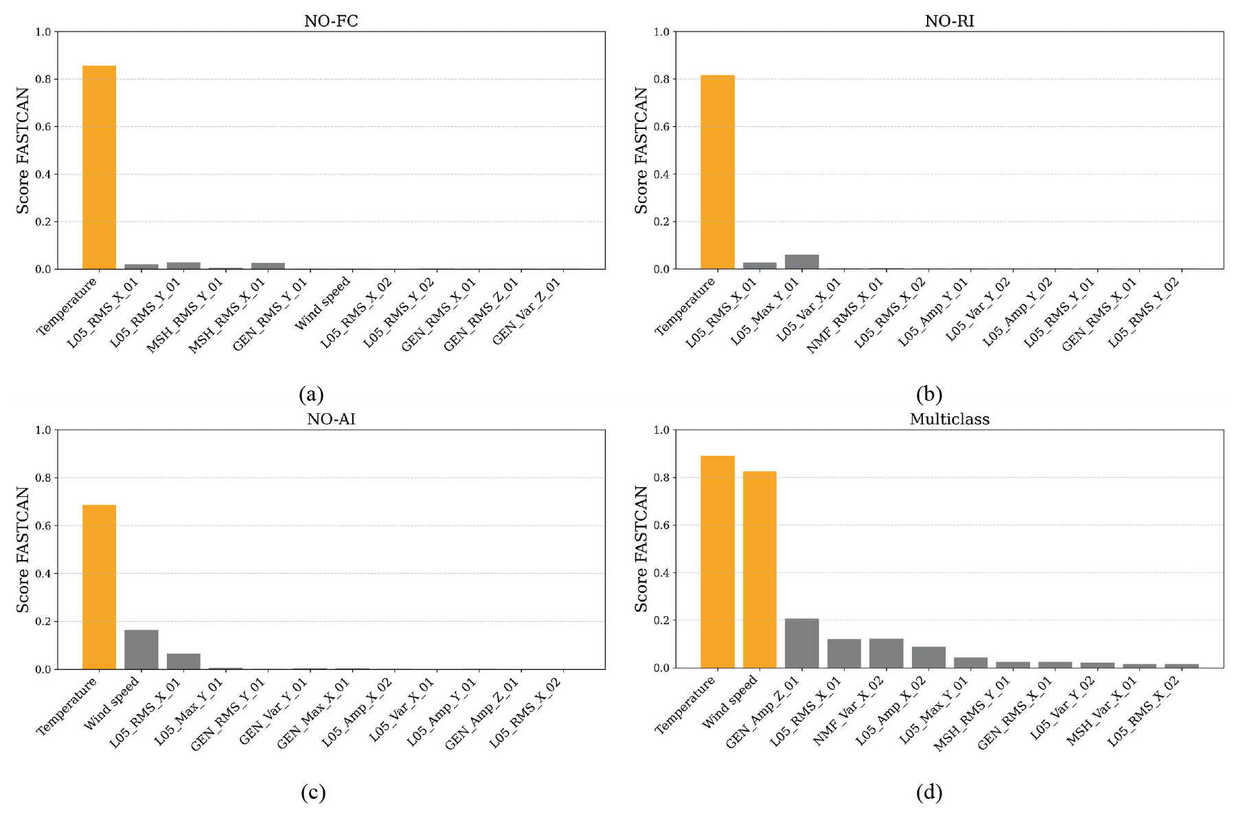
Figure 11 Feature score of the Fe-Sc-kms dataset for (a) NO-FC, (b) NO-RI, (c) NO-AI, and (d) multi-class.

The models' metrics for the Fe-kms-Sc dataset, shown as blue (•) in Fig. 10a–d, indicate the sensitivity of the ML algorithms to the failure classification. The k-means is performed on the structural features, and the SCADA follows its data reorganization, but it is not directly considered in the k-means labelling. For the binary case, the model's metrics range from 0.93 to 0.99. The SVM model reached 0.98 on the NO-FC case, XGBoost reached 0.98 for NO-AI, and XGBoost reached 0.99 for NO-RI. The multi-class case varied from 0.86 by NB to 0.955 by RF. The SCADA data are not included in the Fe-kms dataset, shown as orange (▪) in Fig. 10a–d. The performance metrics reached 0.98 with the SVM model for the NO-FC case, 0.955 with RF for the NO-AI case, 0.98 with XGBoost for the NO-RI case, and 0.95 with RF in the multi-class analysis. When the most sensitive sensor for each failure case was removed from the Fe-kms-LoseSensor dataset (yellow ⧫), performance metrics decreased, except for NO-AI, indicating the importance of this sensor's information for monitoring accuracy and model performance. This result also reinforces the fact that the most sensitive sensor is typically located near the damage site. In the NO-AI case, all sensors were positioned on the nacelle and tower. Although these sensors can capture the dynamic effects of blade aero-imbalance, they are distant from the local damage, which reduces their sensitivity to this phenomenon. Consequently, the sensor group primarily captured global structural responses to the fault rather than local damage effects, which explains the variation in performance when one sensor was removed.

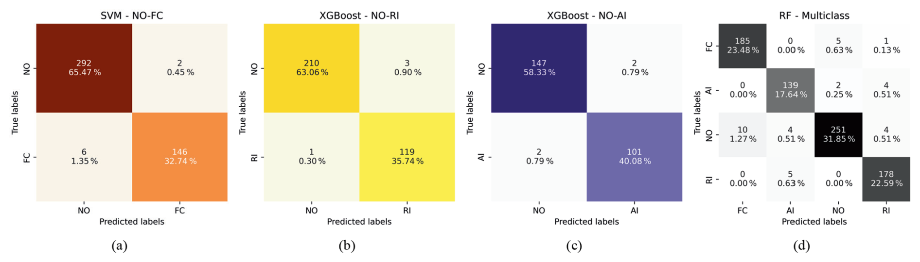
Figure 12 Confusion matrix of binary operational classification for (a) NO-FC, (b) NO-RI, (c) NO-AI, and (d) multi-classification. The dataset assumes the best features plus SCADA data (temperature and wind speed) in each analysis.

The confusion matrices shown in Fig. 12a–c present the results of binary classification using the respective best-performing ML algorithms using the Fe-kms-Sc dataset. In the NO-FC case, the SVM model achieved optimal accuracy and cross-validation, correctly classifying 292 samples as NO (65.47 %) and 146 as FC (32.74 %). For the NO-RI classification, the XGBoost model correctly classifies 210 samples as NO (63.06 %) and 119 as RI (35.74 %). In the NO-AI scenario, the XGBoost model outperformed the others, correctly classifying 101 samples as AI (40.08 %) and 147 as NO (58.33 %). Figure 12d displays the confusion matrix for the multi-class classification involving AI, FC, NO, and RI. The RF model correctly identified 139 samples as AI (17.64 %), 185 as FC (23.48 %), 178 as RI (22.59 %), and 251 as NO (31.85 %).

Among the evaluated configurations, the Fe-kms-Sc dataset provided the most balanced and reliable results for the treated failure identification, including structural and environmental condition information. The dataset Fe-Sc-kms yielded perfect metrics across all models, primarily because environmental parameters, such as temperature and wind speed, were dominant, biasing the classification towards environmental conditions rather than structural responses. In contrast, excluding SCADA data (Fe-kms) enabled the models to capture damage-related structural dynamics more accurately, but it did not account for environmental variability. The Fe-kms-LoseSensor results highlighted the critical role of the most sensitive sensor, typically located near the damage, in maintaining model accuracy. Overall, the Fe-kms-Sc dataset, which integrates structural features with aligned but non-dominant environmental information, yielded the most physically consistent and discriminative performance for the wind turbine failure classification.

5 Conclusions

This study proposes a data-driven hybrid framework for classifying operational conditions of a wind turbine, including normal operation, pitch drive faults, rotor icing, and aerodynamic imbalance, integrating in a hybrid approach multimodal data and multiple ML algorithms. The monitoring process follows this pipeline: data processing and organization, feature extraction, normalization and grouping, clustering, feature and sensor selection, data splitting, machine learning classification, and model evaluation. A novel relative change damage index was introduced to enhance scalability and normalize features extracted from structural dynamic responses and environmental conditions. Canonical correlation analysis was used to identify and rank the most sensitive features among the 15 extracted from temporal responses and SCADA data (wind speed and temperature), and to rank sensors. Thus, multimodal information, including vibration signals from six accelerometers distributed across the turbine and environmental parameters(wind speed and temperature), was incorporated into the framework. Unsupervised k-means clustering enabled the discovery of homogeneous data groups, supporting robust pattern recognition without predefined labels.

Failure classification was implemented as both binary and multi-class tasks using kNN, SVM, DT, RF, Naive Bayes, and XGBoost. Models were tested on the Fe-kms-Sc, Fe-Sc-kms, Fe-kms, and Fe-kms-LoseSensor datasets to evaluate the influence of environmental factors and sensor sensitivity. Using the Fe-kms-Sc dataset, the models performed best, where SVM achieved the highest accuracy for NO-FC (0.98), XGBoost for NO-RI (0.99) and NO-AI (0.98), and RF for multi-class classification (0.955). The Fe-kms-Sc dataset, which combines structural features with aligned SCADA data, yielded the most reliable failure detection. Excluding SCADA data (Fe-kms), the models focused on structural changes, with binary accuracies of 0.93–0.99 and multi-class accuracies of 0.86–0.95. Including SCADA alone (Fe-Sc-kms) produced perfect metrics due to environmental dominance, whereas removing the most sensitive sensor (Fe-kms-LoseSensor) reduced performance, confirming the importance of sensor placement near the damage and identifying the most sensitive sensor in each analysis.

The proposed hybrid model, developed and tested on a 6.7 kW Aventa turbine, effectively manages the complexity of multi-source turbine data and representative fault variations. Its success relies on careful feature and sensor selection, ML model selection, the inclusion of environmental data, dataset multimodality, and thoughtful dataset arrangement, which together enhance discriminative power and classification reliability. However, validation is limited by the small size of the wind turbine, the use of induced faults to simulate aero-imbalance in the blades, and differences between small-scale experimental turbines and large-scale operational turbines or wind farms. Extreme environmental and operational events, such as strong turbulence, large-scale icing, and mixed-fault scenarios, were not included in this study due to the controlled nature and limited scope of the experimental datasets. Ongoing studies aim to evaluate the methodology on larger, more diverse datasets; to further explore environmental effects; to extend the study to offshore wind farms; and to assess the reliability, generalization, and applicability to utility-scale systems.