PhyWakeNet: a dynamic wake model accounting for aerodynamic force oscillations

Advanced wind energy technologies require predictions of the dynamic behaviour of wind turbine wakes. In this work, we present a dynamic wind turbine model, PhyWakeNet, a physics-integrated generative adversarial network-convolutional neural network (GAN-CNN) model for wind turbines under aerodynamic force oscillations. The model combines three interconnected submodels for the time-averaged wake, wake meandering, and small-scale wake turbulence. The time-averaged wake model derives from mass and momentum conservation based on the concept of momentum entrainment, which is computed based on the wake meandering and small-scale wake turbulence models. The wake meandering is captured through conditional GAN-reconstructed spatial modes and a neural-network-enhanced dynamic system for temporal evolution, while the small-scale wake turbulence is generated via a CNN based on the time-averaged wake, wake meandering, and inflow turbulence. The test cases show that the PhyWakeNet model accurately predicts the wake statistics, with the error of the time-averaged velocity deficits, the variance of the streamwise velocity fluctuations, and the wake meandering amplitude to be less than 1 %, 10 %, and 15 %, respectively. Moreover, the model also accurately captures the large-scale temporal variations of instantaneous wake centres and velocity deficits, enabling applications in wake management to mitigate aerodynamic loads and power fluctuations in wind farms.

1 Introduction

Wind turbine wakes significantly impact wind farm performance by reducing power output, increasing aerodynamic loads, and contributing to power output fluctuations (Barthelmie and Jensen, 2010; Stevens and Meneveau, 2017; Meyers et al., 2022). Emerging advancements in wind energy technology (Howland et al., 2022; Meyers et al., 2022) aim at active control of wind turbine wakes to mitigate their negative impacts. This presents new challenges to computational wake modelling, that not only the time-averaged statistics but also the dynamic behaviour of wind turbine wakes need to be captured. However, the modelling capabilities of existing wake models remain limited, with most of them developed for time-averaged wakes. One critical challenge is the incorporation of aerodynamic force oscillations, a critical factor triggering wake meandering (Li et al., 2022b; Messmer et al., 2024) – the most important coherent flow structures in the far wake. In this work, we propose a novel modelling framework that integrates physical principles with advanced machine learning techniques to predict the dynamic behaviour of wind turbine wakes under aerodynamic force oscillations.

Wind turbine wake modelling approaches range from computationally intensive large-eddy simulation (LES) to fast analytical models. LES directly resolves the energy-containing eddies in atmospheric turbulence while modelling subgrid-scale effects on the resolved flow field. For wind turbine wake simulations, blade aerodynamics is typically parameterized through forcing terms to mitigate computational loads (Li et al., 2022d). Despite these parameterizations, the LES of wind turbine wakes still requires substantial computational resources, with simulation times extending from days to weeks depending on the required spatiotemporal resolutions and the spatiotemporal span of interest. This substantial computational demand renders LES currently impractical for wind energy project design and control optimization applications. Analytical wake models, which are often formulated based on the one-dimensional conservation laws, are widely used in wind energy applications because of their computational efficiency. The Jensen model (Jensen, 1983) represents a typical example in this category, which models the variations of downwind velocity deficits through a wake expansion model and an assumed top-hat velocity deficit distribution. To address the limitation of unrealistic top-hat distribution, the following development of analytical models employed different velocity deficit distributions (e.g. Gaussian function or cosine function (Bastankhah and Porté-Agel, 2014; Xie and Archer, 2015; Tian et al., 2015)). Intermediate-fidelity models have also been developed, exemplified by approaches solving simplified Navier–Stokes equations (Ainslie, 1988) and the vortex-based methods (Segalini and Alfredsson, 2013). These mid-fidelity models offer enhanced physical representation by directly resolving additional spatial dimensions, thereby eliminating the need for predefined wake shape assumptions. Despite their advantages, mid-fidelity models share a fundamental limitation with analytical wake models: neither approach can predict dynamic behaviour of wind turbine wakes.

The main coherent flow structure of interest for turbine–turbine interactions is wake meandering, a large-scale low-frequency motion of wind turbine wake in the transverse directions. The most well-known wake meandering model is the dynamic wake meandering (DWM) model developed at Denmark University of Technology (DTU) (Larsen et al., 2008). The DWM model is based on the assumption that the wake can be treated as passive scalars advected by inflow large eddies with the employment of Taylor's frozen flow hypothesis (He et al., 2017). Scale-by-scale turbulence kinetic energy analysis showed that the inflow eddies with the integral length scale greater than ∼3D (where D is the rotor diameter) are effective in advecting wind turbine wakes (Zhang et al., 2023). The shear-layer instability mechanism is another important mechanism for wake meandering. It has been systematically demonstrated using numerical simulations (Mao and Sørensen, 2018; Gupta and Wan, 2019; Li et al., 2022c), wind tunnel experiments (Messmer et al., 2024; Schliffke et al., 2024) and field tests (Angelou et al., 2023). Blade aerodynamics, especially its temporal force oscillations, is a critical factor for the onset and the strength of wake meandering, and is becoming a novel principle for active wake control strategies (Li et al., 2022c; Messmer et al., 2024).

Data-driven approaches have been developed in the literature for wind turbine wake flows – either their mean statistics or instantaneous features. In the work by Ti et al. (Ti et al., 2020), an artificial neural network (ANN) model, trained on RANS-generated datasets, was developed for predicting the mean velocity field. To enable a certain degree of physical interpretability, Gajendran et al. (Gajendran et al., 2023) developed closed-form expressions for predicting time-averaged wake deflection and velocity deficit using a symbolic regression method for yawed wind turbines. The physics-informed neural network (PINN) method was also employed for predicting the time-averaged wake flows. For instance, it was integrated with the k–ϵ turbulence model with an actuator disc representation in Gafoor et al.'s work (Gafoor CTP et al., 2025). Data-driven models for instantaneous wake features are often developed using mode decomposition and machine learning methods. In the work by Zhang and Zhao (Zhang and Zhao, 2020), they proposed a reduced-order model that combines proper orthogonal decomposition (POD) with long short-term memory (LSTM) networks for instantaneous wakes. In the work by Zhou (Zhou et al., 2023), on the other hand, the delayed POD (d-POD) is employed with LSTM. End-to-end models for the entire flow field have also been developed. For instance, He et al. (Li et al., 2022a) developed a bilateral convolutional neural network (BCNN) model, trained on high-fidelity LES datasets, to capture the spatiotemporal evolution of turbine wakes. Despite these advancements, developing data-driven models for instantaneous wakes faces significant challenges. The end-to-end approach has the advantage of capturing a wide range of scales in turbulent wakes. However, such an approach requires large training datasets, which are computationally expensive to generate, to enable a certain degree of generalizability. Modal decomposition-based methods, on the other hand, generally emphasize large-scale coherent structures associated with wake meandering. As a result, small-scale fluctuations are often excessively smoothed, and high-frequency dynamics are not adequately resolved. Moreover, most existing data-driven wake models focused on steady rotor aerodynamics. Consequently, they are inapplicable to wakes of wind turbines subject to dynamic rotor controls and to wakes of floating offshore wind turbines.

To address the above challenges, we develop a novel dynamic wake model, which is dubbed as PhyWakeNet, that synergistically combines physical principles with machine learning methods to compute the spatiotemporal characteristics of wind turbine wakes subject to aerodynamic force oscillations. The proposed model integrates three interconnected submodels: (1) a time-averaged wake model; (2) a wake meandering model; and (3) a model for small-scale turbulence. The key innovative contributions are summarized as follows: (1) introduction of triple velocity decomposition for dynamic wake modelling, which enables scale-specific representations of wake dynamics; (2) accounting for aerodynamic force oscillations in the wake meandering model; and (3) physics-based coupling through the use of the turbulent entrainment concept and the use of coherent structures and inflow turbulence as input features for generating small-scale velocity fluctuations.

2 Methods

The proposed PhyWakeNet model is based on the decomposition of the instantaneous velocity u(x,t) as follows:

$$\begin{array}{}\text{(1)}& \mathit{u}(\mathit{x},t)=\stackrel{\mathrm{‾}}{\mathit{u}}\left(\mathit{x}\right)+\stackrel{\mathrm{̃}}{\mathit{u}}(\mathit{x},t)+{\mathit{u}}^{\prime \prime }(\mathit{x},t),\end{array}$$

where $\stackrel{\mathrm{‾}}{\mathit{u}}$, $\stackrel{\mathrm{̃}}{\mathit{u}}$, and u^′′ denote the time-averaged, wake meandering, and small-scale fluctuating velocity components, respectively. The model requires two primary inputs: the atmospheric flow conditions (C_af) and the turbine operating conditions (particularly control actions for active wake control, also denoted as C_op. C_op (operational conditions) includes the turbine operating and control conditions that may induce unsteady aerodynamic loading and wake modulation. This category encompasses the turbine-thrust-related operating state (e.g. thrust coefficient C_T) as well as control actions capable of introducing aerodynamic force oscillations, such as individual blade pitch control (IBPC) and dynamic yawing. For the cases considered in this study, representative oscillation parameters (e.g. forcing frequency St_F and amplitude A) are briefly indicated here, while their detailed specifications are provided in the case setup section. The velocity field $\mathit{u}=\stackrel{\mathrm{‾}}{\mathit{u}}+\stackrel{\mathrm{̃}}{\mathit{u}}+{\mathit{u}}^{\prime \prime }$ constitutes the model output. The time-averaged velocity field $\stackrel{\mathrm{‾}}{\mathit{u}}\left(\mathit{x}\right)$ is derived from mass and momentum conservation principles. The wake meandering component $\stackrel{\mathrm{̃}}{\mathit{u}}(\mathit{x},t)$ is modelled through (1) a conditional generative adversarial network (CGAN) for the dominant spatial modes and (2) a data-driven dynamical system for temporal evolution. The small-scale velocity fluctuations ${\mathit{u}}^{\prime \prime }(\mathit{x},t)$ are generated by a convolutional neural network (CNN) that takes both the inflow conditions, and time-averaged and wake meandering flow field as inputs. The coupling of the three submodels is enabled by both physical insights and machine learning methods. A key challenge is to quantify the enhanced wake–ambient flow mixing induced by active wake control strategies, which is modelled based on the momentum entrainment concept, quantifying the combined effects of wake meandering and small-scale velocity fluctuations on wake recovery. In the following of the paper, u, v, and w represent the streamwise, spanwise, and vertical velocity components, respectively. The fluctuating components are collectively denoted as ${\mathit{u}}^{\prime }(\mathit{x},t)=\stackrel{\mathrm{̃}}{\mathit{u}}(\mathit{x},t)+{\mathit{u}}^{\prime \prime }(\mathit{x},t)$. A schematic of the PhyWakeNet model is provided in Fig. 1.

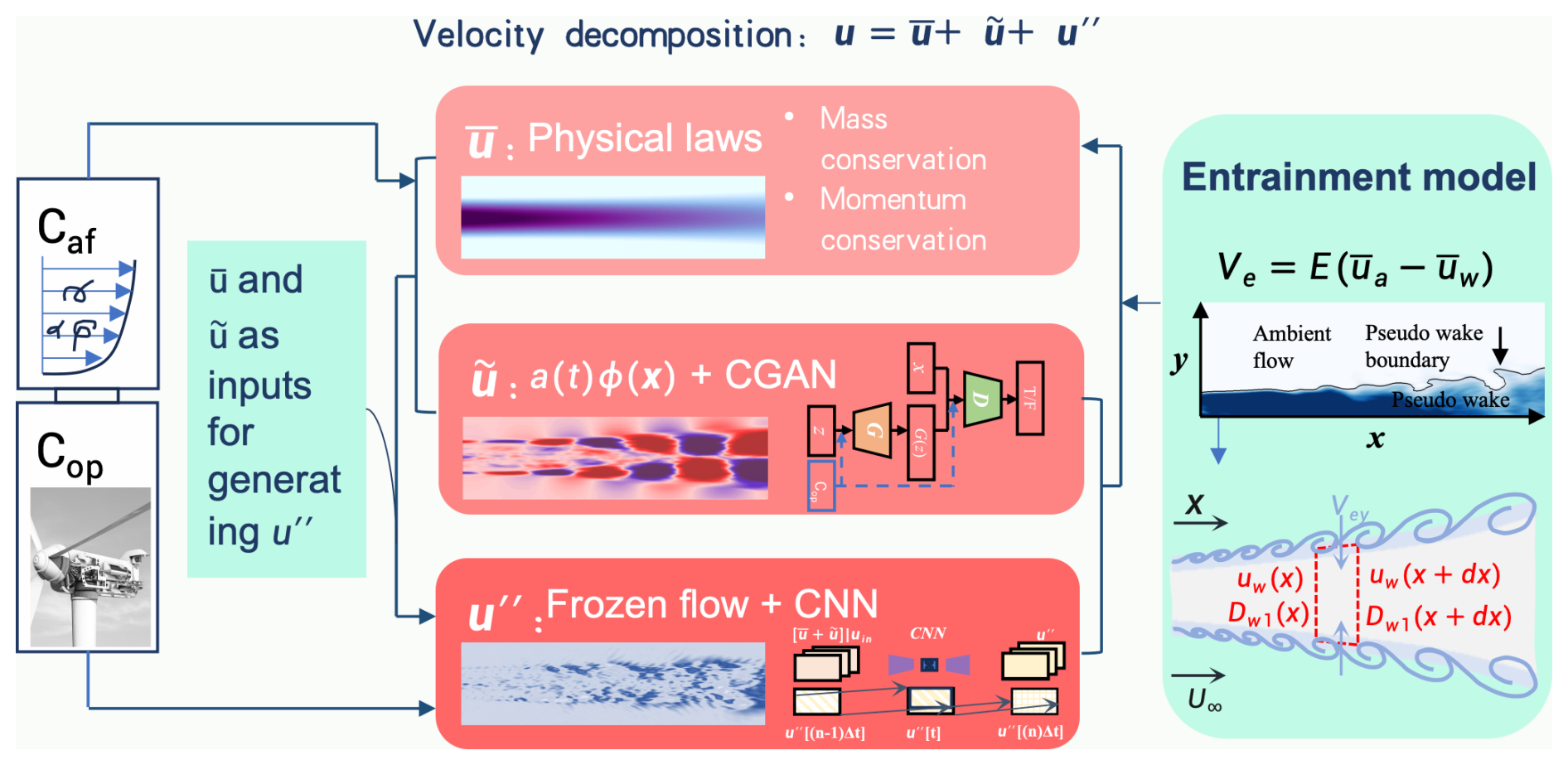
Figure 1 Schematic of the proposed PhyWakeNet model including three submodels for the time-averaged, meandering, and small-scale turbulence of wind turbine wakes. The inputs include the atmospheric flow conditions and the turbine operational conditions. The output is the spatiotemporal variation of velocity field. The time-averaged wake flow is modelled based on the mass and momentum conservation. The wake meandering and small-scale turbulence are modelled using CGAN and CNN. The impacts of wake meandering and small-scale turbulence on time-averaged wake are modelled based on the momentum entrainment model. The outputs from the time-averaged wake model and the wake meandering model are employed for the construction of small-scale turbulence.

2.1 Time-averaged wake model

2.1.1 Governing equations

The time-averaged wake flow model is formulated based on mass and momentum conservation, predicting both velocity deficit and wake width evolution along the wind turbine downstream direction. This model incorporates enhanced mass and momentum fluxes resulting from wake meandering and small-scale velocity fluctuations through an entrainment model. Specifically, the following mass and momentum conservation equations are employed:

$$\begin{array}{}\text{(2)}& \left\{\begin{array}{l}{\displaystyle \frac{\mathrm{d}\left(A_{\mathrm{w}}{\stackrel{\mathrm{‾}}{u}}_{\mathrm{w}}\right)}{\mathrm{d}x}}=V_{\mathrm{e}}{S}_{\mathrm{w}}\\ {\displaystyle \frac{\mathrm{d}\left(A_{\mathrm{w}}{\stackrel{\mathrm{‾}}{u}}_{\mathrm{w}}^{\mathrm{2}}\right)}{\mathrm{d}x}}=V_{\mathrm{e}}{S}_{\mathrm{w}}{\stackrel{\mathrm{‾}}{u}}_{\mathrm{a}},\end{array}\right.\end{array}$$

where A_w is the wake cross-sectional area normal to the centreline, ${\stackrel{\mathrm{‾}}{u}}_{\mathrm{w}}$ is the mean streamwise wake velocity, S_w represents the wake–ambient flow interface area per unit downwind distance, V_e is the entrainment velocity, ${\stackrel{\mathrm{‾}}{u}}_{\mathrm{a}}$ is the ambient mean streamwise velocity. The entrainment velocity V_e is computed through the entrainment coefficient E,

$$\begin{array}{}\text{(3)}& V_{\mathrm{e}}=E({\stackrel{\mathrm{‾}}{u}}_{\mathrm{a}}-{\stackrel{\mathrm{‾}}{u}}_{\mathrm{w}}),\end{array}$$

where E quantifies the rate at which ambient fluid is entrained into the wake. The entrainment approach represents a well-established method for modelling the development of highly turbulent regions into relatively quiescent ambient flows (Morton et al., 1956). For wind turbine wake modelling specifically, it has been employed in the work by Luzzatto-Fegiz (Luzzatto-Fegiz, 2018).

The wake's cross-sectional shape is modelled as an ellipse with major axis D_w1 and minor axis D_w2 to capture the directional effects of aerodynamic force oscillations on wake meandering preferences.

Consistent with this elliptical assumption, we postulate that the wake growth rates along both principal directions scale with the ratio of their respective entrainment coefficients, while the entrainment coefficient itself follows an elliptical distribution. These considerations yield the following final governing equations:

$$\begin{array}{}\text{(4)}& \left\{\begin{array}{l}{\displaystyle \frac{\mathrm{d}\left({\displaystyle \frac{\mathit{\pi }}{\mathrm{4}}}{D}_{\mathrm{w}\mathrm{1}}{D}_{\mathrm{w}\mathrm{2}}{\stackrel{\mathrm{‾}}{u}}_{\mathrm{w}}\right)}{\mathrm{d}x}}\\ =\underset{\mathrm{0}}{\overset{\mathrm{2}\mathit{\pi }}{\int }}E\left(\mathit{\theta }\right)(U_{\mathrm{a}}-U_{\mathrm{w}})\cos (\mathit{\alpha }-\mathit{\theta })r\mathrm{d}\mathit{\theta },\\ {\displaystyle \frac{\mathrm{d}\left({\displaystyle \frac{\mathit{\pi }}{\mathrm{4}}}{D}_{\mathrm{w}\mathrm{1}}{D}_{\mathrm{w}\mathrm{2}}{\stackrel{\mathrm{‾}}{u}}_{\mathrm{w}}^{\mathrm{2}}\right)}{\mathrm{d}x}}\\ =\underset{\mathrm{0}}{\overset{\mathrm{2}\mathit{\pi }}{\int }}E\left(\mathit{\theta }\right)(U_{\mathrm{a}}-U_{\mathrm{w}})U_{\mathrm{a}}\cos (\mathit{\alpha }-\mathit{\theta })r\mathrm{d}\mathit{\theta },\\ {\displaystyle \frac{\mathrm{d}{D}_{\mathrm{w}\mathrm{1}}}{\mathrm{d}x}}/{\displaystyle \frac{\mathrm{d}{D}_{\mathrm{w}\mathrm{2}}}{\mathrm{d}x}}=E_{\mathrm{1}}/E_{\mathrm{2}}.\end{array}\right.\end{array}$$

Here, E₁ and E₂ denote the entrainment constants along the major and minor axes, respectively, with the angular dependence $E\left(\mathit{\theta }\right)=\sqrt{E_{\mathrm{1}}^{\mathrm{2}}{\cos }^{\mathrm{2}}\mathit{\theta }+E_{\mathrm{2}}^{\mathrm{2}}{\sin }^{\mathrm{2}}\mathit{\theta }}$. The angles α and θ are illustrated in Fig. 2, α is the angle between the normal to the ellipse at the set point and the major axis, and θ is the angle between the line connecting the set point and the centre of the ellipse and the major axis.

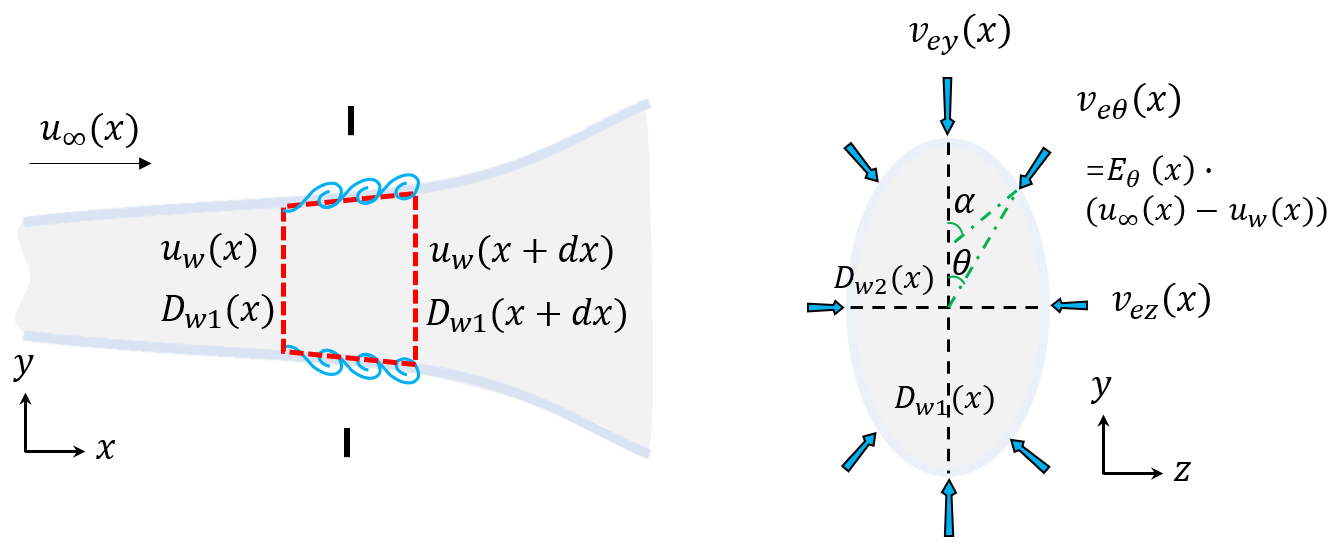
Figure 2 Schematic of the time-averaged wake flow model. The left panel shows the wake profile in the hub-height x–y plane, while the right panel displays the wake cross-section in the y–z plane. Arrows indicate ambient flow entrainment. The wake cross-section is modelled as an ellipse (right panel), with aerodynamic force oscillations assumed to act in the y direction.

To solve the governing equations, initial conditions for both the streamwise velocity and wake diameter at the near-wake position are required. In this work, these are determined using one-dimensional momentum theory,

$$\begin{array}{}\text{(5)}& \left\{\begin{array}{l}{\stackrel{\mathrm{‾}}{u}}_{\mathrm{w}}=(\mathrm{1}-\mathrm{2}a){\stackrel{\mathrm{‾}}{u}}_{\text{in}}\\ D_{\mathrm{w}\mathrm{1}}=D_{\mathrm{w}\mathrm{2}}=D,\end{array}\right.\end{array}$$

at the 1D downstream position. Here, ${\stackrel{\mathrm{‾}}{u}}_{\text{in}}$ represents the incoming wind speed (which may differ from the ambient wind speed ${\stackrel{\mathrm{‾}}{u}}_{\mathrm{a}}$ for turbines operating in an array), and a denotes the axial induction factor. The induction factor relates to the thrust coefficient C_T through the expression $a=\frac{\mathrm{1}-\sqrt{\mathrm{1}-C_{\mathrm{T}}}}{\mathrm{2}}$.

It should be noted that the governing equations presented above only provide the mean velocity deficit. To characterize the spatial distribution, we assume that the isocontours of ${\stackrel{\mathrm{‾}}{u}}_{\mathrm{w}}$ follow an elliptical pattern, with the velocity deficit profile described by a cosine function along the major and minor axes:

$$\begin{array}{}\text{(6)}& \left\{\begin{array}{l}u\left(y\right)={\stackrel{\mathrm{‾}}{u}}_{\mathrm{c}}\cos \left(\mathit{\pi }y/D_{\mathrm{c}}\right)\\ u\left(z\right)={\stackrel{\mathrm{‾}}{u}}_{\mathrm{c}}\cos \left(\mathit{\pi }z/D_{cz}\right).\end{array}\right.\end{array}$$

The parameters ${\stackrel{\mathrm{‾}}{u}}_{\mathrm{c}}$ and D_c are determined by enforcing conservation of mass and momentum fluxes before and after the transformation:

$$\begin{array}{}\text{(7)}& \left\{\begin{array}{l}{A}_{\mathrm{w}}(\mathrm{1}-{\stackrel{\mathrm{‾}}{u}}_{\mathrm{w}})=\int {\stackrel{\mathrm{‾}}{u}}_{\mathrm{c}}\cos \left(\mathit{\pi }y/D_c\right)\mathrm{d}{A}_{cy}\\ A_{\mathrm{w}}(\mathrm{1}-{\stackrel{\mathrm{‾}}{u}}_{\mathrm{w}}{)}^{\mathrm{2}}=\int {\left({\stackrel{\mathrm{‾}}{u}}_{\mathrm{c}}\cos \left(\mathit{\pi }y/D_c\right)\right)}^{\mathrm{2}}\mathrm{d}{A}_{cy}.\end{array}\right.\end{array}$$

Substituting the specific parameters yields the concrete form of these equations:

$$\begin{array}{}\text{(8)}& \left\{\begin{array}{l}{\displaystyle \frac{\mathit{\pi }}{\mathrm{4}}}(\mathrm{1}-{\stackrel{\mathrm{‾}}{u}}_{\mathrm{w}})D_{\mathrm{w}\mathrm{1}}{D}_{\mathrm{w}\mathrm{2}}\\ =\underset{\mathrm{0}}{\overset{D_c/\mathrm{2}}{\int }}\mathit{\pi }{\stackrel{\mathrm{‾}}{u}}_{\mathrm{c}}\cos \left(\mathit{\pi }y/D_c\right)(\mathrm{1}+D_{\mathrm{w}\mathrm{2}}/D_{\mathrm{w}\mathrm{1}})y\mathrm{d}y\\ {\displaystyle \frac{\mathit{\pi }}{\mathrm{4}}}(\mathrm{1}-{\stackrel{\mathrm{‾}}{u}}_{\mathrm{w}}{)}^{\mathrm{2}}{D}_{\mathrm{w}\mathrm{1}}{D}_{\mathrm{w}\mathrm{2}}\\ =\underset{\mathrm{0}}{\overset{D_c/\mathrm{2}}{\int }}\mathit{\pi }{\left({\stackrel{\mathrm{‾}}{u}}_{\mathrm{c}}\cos \left(\mathit{\pi }y/D_c\right)\right)}^{\mathrm{2}}(\mathrm{1}+D_{\mathrm{w}\mathrm{2}}/D_{\mathrm{w}\mathrm{1}})y\mathrm{d}y.\end{array}\right.\end{array}$$

Solving these equations leads to analytical expressions for ${\stackrel{\mathrm{‾}}{u}}_{\mathrm{c}}$ and D_c:

$$\begin{array}{}\text{(9)}& \left\{\begin{array}{l}{\stackrel{\mathrm{‾}}{u}}_{\mathrm{c}}={\displaystyle \frac{\mathrm{8}(\mathrm{1}-{\stackrel{\mathrm{‾}}{u}}_{\mathrm{w}})}{\mathit{\pi }+\mathrm{2}}}\\ D_{\mathrm{c}}=\sqrt{{\displaystyle \frac{{\mathit{\pi }}^{\mathrm{2}}(\mathit{\pi }+\mathrm{2})}{\mathrm{32}(\mathit{\pi }-\mathrm{2})}}}{D}_{\mathrm{w}\mathrm{1}}.\end{array}\right.\end{array}$$

A note is that the wake width in this new distribution differs from that under a uniform distribution. With ${\stackrel{\mathrm{‾}}{u}}_{\text{in}}$ and a specified, the governing equations for the time-averaged wake statistics (${\stackrel{\mathrm{‾}}{u}}_{\mathrm{w}}$, D_w1, D_w2) form a closed system when combined with the entrainment coefficient model.

2.1.2 Wake entrainment model

The detailed theoretical derivation of the estimation method for parameter E is given in this section. Ambient turbulence and wake shear layer constitute the primary drivers of mass and momentum entrainment across the wake boundary. This physical understanding leads to the following formulation for the total entrainment coefficient:

$$\begin{array}{}\text{(10)}& E=E_{\text{a}}+E_{\text{s}}=E_{\text{a}}+{\displaystyle \frac{\langle v_{\mathrm{e}}{A}_{\mathit{\eta }}\rangle }{\langle v_{\mathrm{e},o}{A}_{\mathit{\eta },o}\rangle }}{E}_{\mathrm{s},o},\end{array}$$

where E_a and E_s represent contributions from ambient turbulence and wake shear-layer effects, respectively. The angle brackets 〈⋅〉 indicate time-averaged quantities. Subscript o denotes reference values corresponding to conditions without active wake control, obtainable through either numerical simulations or experimental measurements. The ambient turbulence component E_a is treated as a known input parameter. The model accounts for enhanced entrainment through proportionality to both the entrainment velocity v_e and the wake–ambient interface area A_η, the latter being directly computed from the modelled flow fields $\stackrel{\mathrm{̃}}{\mathit{u}}$ and u^′′.

The entrainment velocity v_e remains the only quantity requiring modelling in this formulation. To approximate v_e, we first establish the wake boundary as the iso-surface of streamwise velocity deficit Δu. The material derivative of Δu at an arbitrary point in the flow field is given by

$$\begin{array}{}\text{(11)}& {\displaystyle \frac{D\mathrm{\Delta }u}{Dt}}={\displaystyle \frac{\partial \mathrm{\Delta }u}{\partial t}}+\mathit{u}\cdot \mathrm{\nabla }\mathrm{\Delta }u.\end{array}$$

At the wake boundary, where the material derivative vanishes, this relationship simplifies to

$$\begin{array}{}\text{(12)}& \mathrm{0}={\displaystyle \frac{\partial \mathrm{\Delta }u}{\partial t}}+{\mathit{u}}_{\mathit{\eta }}\cdot \mathrm{\nabla }\mathrm{\Delta }u,\end{array}$$

where u_η represents the velocity of the wake boundary. The entrainment velocity is subsequently defined as the relative velocity component normal to this boundary:

$$\begin{array}{}\text{(13)}& v_{\mathrm{e}}=\left(\mathit{u}-{\mathit{u}}_{\mathit{\eta }}\right)\cdot {\mathit{e}}_{\mathrm{n}},\end{array}$$

with e_n denoting the unit normal vector to the wake boundary. By subtracting Eq. (12) from Eq. (11), we derive the following expression for V_e:

$$\begin{array}{}\text{(14)}& v_{\mathrm{e}}=-{\left[{\displaystyle \frac{\mathrm{1}}{\left|\mathrm{\nabla }\mathrm{\Delta }u\right|}}{\displaystyle \frac{D\mathrm{\Delta }u}{Dt}}\right]}_{\mathit{\eta }}.\end{array}$$

While this formulation theoretically enables direct computation of v_e, practical implementation presents challenges due to both computational complexity and the frequent unavailability of instantaneous velocity deficit field snapshots.

In what follows, we demonstrate that the entrainment velocity can be approximated using the time derivative of the wake centre position in the transverse direction. The entrainment velocity is first expressed as

$$\begin{array}{ll}\text{(15)}& {\displaystyle }{v}_{\mathrm{e}}& {\displaystyle }=-{\left[{\displaystyle \frac{\mathrm{1}}{\left|\mathrm{\nabla }\right(\mathrm{\Delta }u\left)\right|}}{\displaystyle \frac{D\left(\mathrm{\Delta }u\right)}{Dt}}\right]}_{\mathit{\eta }}{\displaystyle }& {\displaystyle }=-\left[{\displaystyle \frac{\mathrm{1}}{\sqrt{{\left(\frac{\partial \left(\mathrm{\Delta }u\right)}{\partial x}\right)}^{\mathrm{2}}+{\left(\frac{\partial \left(\mathrm{\Delta }u\right)}{\partial y}\right)}^{\mathrm{2}}}}}\right.\\ \text{(16)}& {\displaystyle }& {\displaystyle }{\left.\cdot \left({\displaystyle \frac{\partial \left(\mathrm{\Delta }u\right)}{\partial t}}+u{\displaystyle \frac{\partial \left(\mathrm{\Delta }u\right)}{\partial x}}+v{\displaystyle \frac{\partial \left(\mathrm{\Delta }u\right)}{\partial y}}\right)\right]}_{\mathit{\eta }}.\end{array}$$

For slender wakes, where both the transverse velocity component v and the streamwise gradient $\partial \mathrm{\Delta }u/\partial x$ remain small, this expression simplifies to

$$\begin{array}{}\text{(17)}& v_{\mathrm{e}}\approx -{\left[{\left({\displaystyle \frac{\partial \left(\mathrm{\Delta }u\right)}{\partial y}}\right)}^{-\mathrm{1}}{\displaystyle \frac{\partial \left(\mathrm{\Delta }u\right)}{\partial t}}\right]}_{\mathit{\eta }}.\end{array}$$

The transverse wake centre position is defined as

$$\begin{array}{}\text{(18)}& y_{\mathrm{c}}(x,t)={\displaystyle \frac{{\int }_{{\mathit{\eta }}_{\mathrm{l}}\left(t\right)}^{{\mathit{\eta }}_u\left(t\right)}\mathrm{\Delta }u(x,y,t)y\mathrm{d}y}{{\int }_{{\mathit{\eta }}_{\mathrm{l}}\left(t\right)}^{{\mathit{\eta }}_u\left(t\right)}\mathrm{\Delta }u(x,y,t)\mathrm{d}y}},\end{array}$$

where η_l(t) and η_u(t) denote the transverse y coordinates of the lower and upper wake boundaries, respectively. Introducing the cumulative velocity deficit function $F(y,t)={\int }_{-\mathrm{\infty }}^{\mathit{\eta }}\mathrm{\Delta }u(x,y,t)\mathrm{d}y$, this expression transforms to

$$\begin{array}{}\text{(19)}& y_{\mathrm{c}}(x,t)={\displaystyle \frac{F(y,t)y{|}_{{\mathit{\eta }}_{\mathrm{l}}\left(t\right)}^{{\mathit{\eta }}_u\left(t\right)}-{\int }_{{\mathit{\eta }}_{\mathrm{l}}\left(t\right)}^{{\mathit{\eta }}_u\left(t\right)}F(y,t)\mathrm{d}y}{F(y,t){|}_{{\mathit{\eta }}_{\mathrm{l}}\left(t\right)}^{{\mathit{\eta }}_u\left(t\right)}}}.\end{array}$$

Recognizing that $F({\mathit{\eta }}_l,t)=\mathrm{0}$ by definition, we obtain the simplified form

$$\begin{array}{}\text{(20)}& y_{\mathrm{c}}(x,t)={\mathit{\eta }}_u\left(t\right)-{\displaystyle \frac{{\int }_{{\mathit{\eta }}_{\mathrm{l}}\left(t\right)}^{{\mathit{\eta }}_u\left(t\right)}F(y,t)\mathrm{d}y}{F\left({\mathit{\eta }}_u\left(t\right),t\right)}}.\end{array}$$

The temporal evolution of the wake centre position follows from differentiation

$$\begin{array}{}\text{(21)}& {\displaystyle \frac{\mathrm{d}{y}_{\mathrm{c}}(x,t)}{\mathrm{d}t}}={\displaystyle \frac{\mathrm{d}{\mathit{\eta }}_u\left(t\right)}{\mathrm{d}t}}-{\displaystyle \frac{\mathrm{d}}{\mathrm{d}t}}\left({\displaystyle \frac{{\int }_{{\mathit{\eta }}_{\mathrm{l}}\left(t\right)}^{{\mathit{\eta }}_u\left(t\right)}F(y,t)\mathrm{d}y}{F\left({\mathit{\eta }}_u\right(t),t)}}\right).\end{array}$$

Under the assumption that velocity deficit integrals remain approximately stationary, this simplifies to

$$\begin{array}{}\text{(22)}& {\displaystyle \frac{\mathrm{d}{y}_{\mathrm{c}}(x,t)}{\mathrm{d}t}}\approx {\displaystyle \frac{\mathrm{d}{\mathit{\eta }}_u\left(t\right)}{\mathrm{d}t}}.\end{array}$$

At the upper wake boundary, where $\mathrm{\Delta }u\left({\mathit{\eta }}_u\right(t),t)=C$ remains constant, differentiation yields

$$\begin{array}{}\text{(23)}& \mathrm{0}={\displaystyle \frac{\partial \left(\mathrm{\Delta }u\right)}{\partial {\mathit{\eta }}_u}}{\displaystyle \frac{\mathrm{d}{\mathit{\eta }}_u}{\mathrm{d}t}}+{\displaystyle \frac{\partial \left(\mathrm{\Delta }u\right)}{\partial t}}.\end{array}$$

Combining Eqs. (17), (22), and (23), and assuming $\partial \left(\mathrm{\Delta }u\right)/\partial {\mathit{\eta }}_u\approx \partial \left(\mathrm{\Delta }u\right)/\partial y$, we derive the entrainment velocity approximation

$$\begin{array}{}\text{(24)}& v_{\mathrm{e}}\approx {\displaystyle \frac{\mathrm{d}{y}_{\mathrm{c}}}{\mathrm{d}t}}.\end{array}$$

This leads to the final expression for the entrainment coefficient

$$\begin{array}{}\text{(25)}& \begin{array}{rl}E& =E_a+{\displaystyle \frac{\langle (\mathrm{d}{y}_{\mathrm{c}}/\mathrm{d}t)A_{\mathit{\eta }}\rangle }{\langle (\mathrm{d}{y}_{\mathrm{c}}/\mathrm{d}t{)}_o{A}_{\mathit{\eta },o}\rangle }}{E}_{\mathrm{s},o}\\ & \approx E_a+{\displaystyle \frac{(\mathrm{d}{y}_{\mathrm{c}}/\mathrm{d}t{)}_{\text{max}}\langle A_{\mathit{\eta }}\rangle }{\left[\right(\mathrm{d}{y}_{\mathrm{c}}/\mathrm{d}t{)}_f{]}_{\text{max}}\langle A_{\mathit{\eta },o}\rangle }}{E}_{\mathrm{s},o}.\end{array}\end{array}$$

In the second formulation, the instantaneous $\mathrm{d}{y}_{\mathrm{c}}/\mathrm{d}t$ is replaced by its temporal maximum to avoid computing the product with A_η. The reference quantities $(\mathrm{d}{y}_{\mathrm{c}}/\mathrm{d}t{)}_o$, A_η,o, and E_s,o are derived from LES data: the first two are computed directly from simulations, while E_s,o is obtained through least-squares fitting of the velocity deficit to Eq. (2). Notably, E varies spatially in oscillating turbine wakes due to the downstream evolution of A_η.

To ensure physical consistency and numerical robustness, we have revised Eq. (25) by introducing a characteristic reference scale Φ_ref=α(U_∞D²):

$$\begin{array}{}\text{(26)}& \begin{array}{rl}E& =E_a+{\displaystyle \frac{\langle (\mathrm{d}{y}_{\mathrm{c}}/\mathrm{d}t)A_{\mathit{\eta }}\rangle }{\langle (\mathrm{d}{y}_{\mathrm{c}}/\mathrm{d}t{)}_o{A}_{\mathit{\eta },o}\rangle }}{E}_{\mathrm{s},o}\\ & \approx E_a+{\displaystyle \frac{(\mathrm{d}{y}_{\mathrm{c}}/\mathrm{d}t{)}_{\text{max}}\langle A_{\mathit{\eta }}\rangle +{\mathrm{\Phi }}_{\mathrm{ref}}}{\left[\right(\mathrm{d}{y}_{\mathrm{c}}/\mathrm{d}t{)}_f{]}_{\text{max}}\langle A_{\mathit{\eta },o}\rangle +{\mathrm{\Phi }}_{\mathrm{ref}}}}{E}_{\mathrm{s},o}.\end{array}\end{array}$$

The parameter α is set to 10⁻³ to represent the intrinsic physical floor of the baseline flow. This ensures numerical stability in the near wake while remaining sufficiently small to preserve the model's sensitivity to the relative entrainment enhancement triggered by aerodynamic oscillations.

2.2 Wake meandering model

The coherent flow structures in the wake, represented by the leading spectral proper orthogonal decomposition (SPOD) modes, are modelled using a CGAN model, with their temporal evolution captured by a data-driven dynamical system. Specifically, the coherent velocity $\stackrel{\mathrm{̃}}{\mathit{u}}$ is expressed as

$$\begin{array}{}\text{(27)}& \stackrel{\mathrm{̃}}{\mathit{u}}(C_{\text{af}},C_{\text{op}},\mathit{x},t)\approx \sum _{i=\mathrm{1}}^N{a}_i(C_{\text{af}},C_{\text{op}},t){\mathbf{\Phi }}_i\left(C_{\text{af}},C_{\text{op}},\mathit{x}\right),\end{array}$$

where Φ_i represents the SPOD modes and a_i denotes the corresponding temporal coefficients, with N being the number of leading SPOD modes employed for coherent flow construction. Both Φ_i and a_i depend on C_af, the atmospheric flow condition, and C_op, the wind turbine operational condition. A schematic of the coherent wake flow model is shown in Fig. 3.

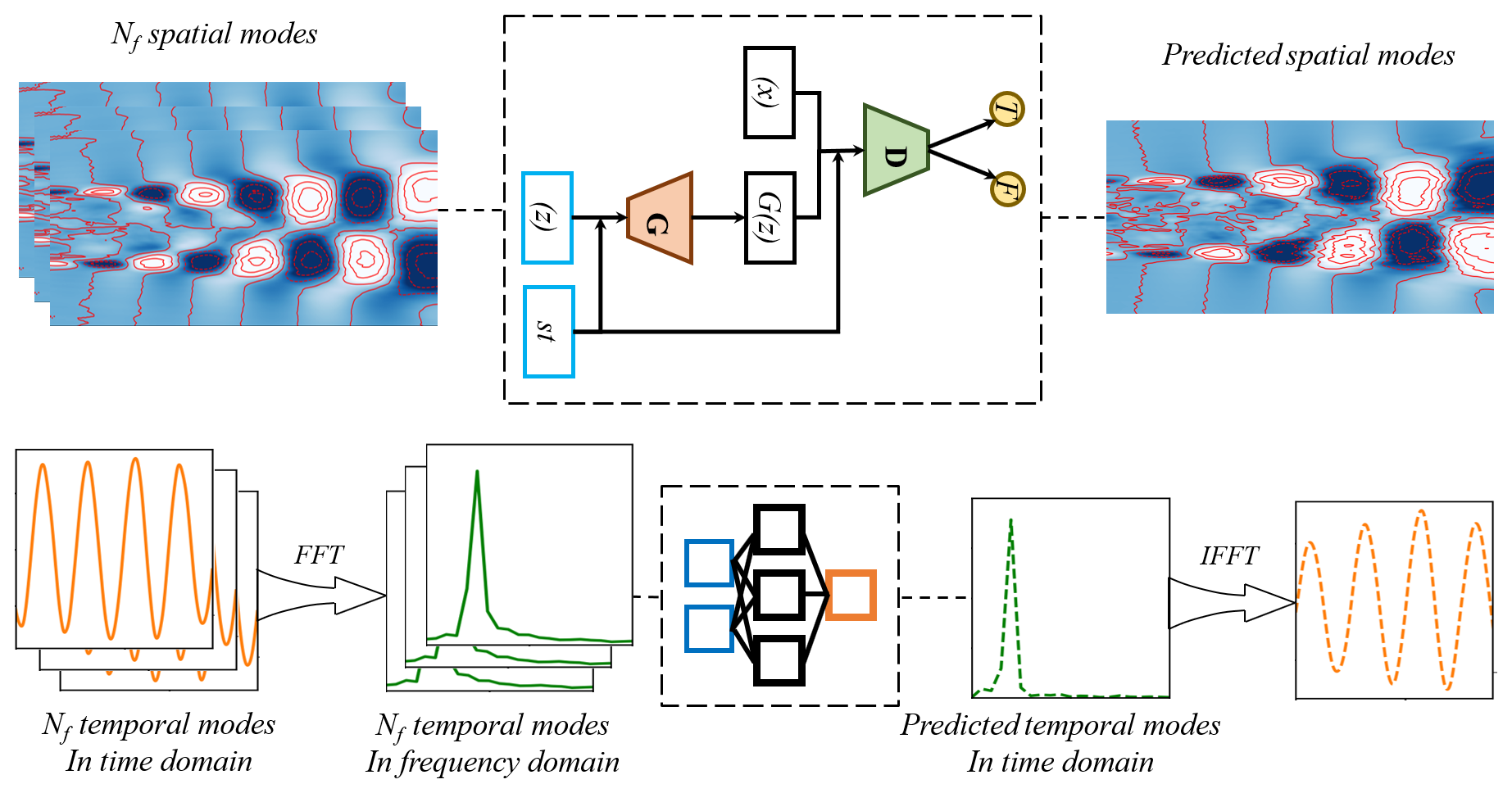
Figure 3 Conceptual diagram of the coherent wake flow model. The upper portion illustrates the generation of spatial modes, while the lower portion shows the model for temporal evolutions.

2.2.1 Model for spatial modes

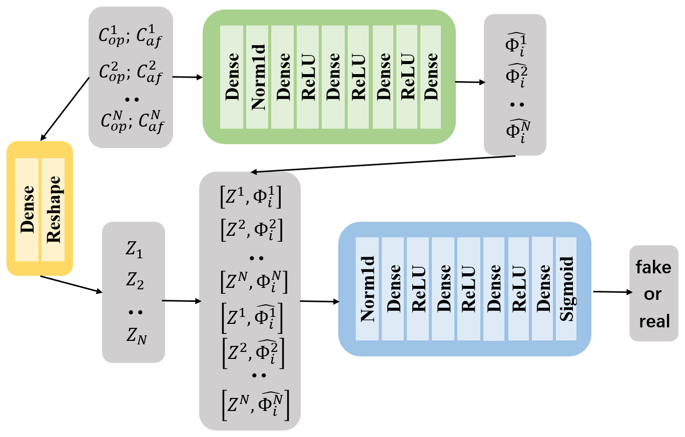
This section presents the modelling approach for the SPOD modes Φ_i. The conditional generative adversarial network (CGAN) generates the ith SPOD mode for specified conditions C_af and C_op according to the following expression:

$$\begin{array}{}\text{(28)}& \begin{array}{rl}{\mathbf{\Phi }}_i\left(C_{\text{af}},C_{\text{op}},\mathit{x}\right)& ={\mathbf{\Phi }}_{\text{NN}}\left(C_{\text{af}},C_{\text{op}},{\mathbf{\Phi }}_i^{\mathrm{1}}\left(C_{\text{af}}^{\mathrm{1}},C_{\text{op}}^{\mathrm{1}},\mathit{x}\right),\right.\\ & \left.{\mathbf{\Phi }}_i^{\mathrm{2}}\left(C_{\text{af}}^{\mathrm{2}},C_{\text{op}}^{\mathrm{2}},\mathit{x}\right),\mathrm{\dots }\right),\end{array}\end{array}$$

where Φ_NN denotes the neural network model trained on multiple realizations of the ith SPOD mode, ${\mathbf{\Phi }}_i^j$ ($j=\mathrm{1},\mathrm{2},\mathrm{\dots }$), under different conditions $C^{j_{\text{af}}}$ and $C^{j_{\text{op}}}$. The model uses C_af and C_op as input features. This formulation implicitly assumes that the ith mode depends exclusively on corresponding modes from various conditions, without explicit consideration of interactions with other modes.

The CGAN model for generating spatial modes comprises two components (Fig. 4): a generator and a discriminator. The generator accepts the operating conditions C_af and C_op as inputs and produces predicted spatial modes Φ_NN. The discriminator evaluates input pairs consisting of operating conditions (C_af, C_op) and corresponding spatial modes (Φ_NN), outputting a binary classification (real or fake). During training, the discriminator's weights remain fixed while only the generator's weights undergo updates. After training completion, the generator functions as a surrogate model for predicting spatial modes under arbitrary atmospheric and operational conditions.

Figure 4 Schematic of the CGAN model for generating spatial modes.

2.2.2 Temporal evolution model

This section describes the model for the temporal coefficients a_i of the SPOD modes. The temporal evolution of coherent flow structures is modelled through a dynamic system representation for $a_i(C_{\text{af}},C_{\text{op}},t)$, expressed as

$$\begin{array}{}\text{(29)}& {\displaystyle \frac{\mathrm{d}{a}_i}{\mathrm{d}t}}=f_i,\end{array}$$

where f_i represents the forcing term modelled using a deep neural network (DNN). The forcing term construction involves two sequential steps: first generating sample temporal coefficients for each SPOD mode under specified conditions C_af and C_op, followed by constructing the forcing term using these generated coefficients. The sample temporal coefficients derive from corresponding frequency spectra models for each SPOD mode, which are themselves modelled using neural networks trained on frequency spectra datasets across various operational conditions:

$$\begin{array}{}\text{(30)}& \begin{array}{rl}{S}_{a_i}\left(C_{\text{af}},C_{\text{op}},\mathit{\omega }\right)& ={\text{DNN}}_S\left(C_{\text{af}},C_{\text{op}},S_{a_i}^{\mathrm{1}}\left(C_{\text{af}}^{\mathrm{1}},C_{\text{op}}^{\mathrm{1}},\mathit{\omega }\right)\right.\\ & \left.S_{a_i}^{\mathrm{2}}\left(C_{\text{af}}^{\mathrm{2}},C_{\text{op}}^{\mathrm{2}},\mathit{\omega }\right),\mathrm{\dots }\right),\end{array}\end{array}$$

where ω denotes frequency, $S_{a_i}$ represents the frequency spectrum for the ith SPOD mode under conditions C_af and C_op, and DNN_S constitutes the neural network model approximating the frequency spectrum. This model employs datasets of frequency spectra ($S_{a_i}^{\mathrm{1}},S_{a_i}^{\mathrm{2}},\mathrm{\dots }$) from various conditions while maintaining the same fundamental assumption as the SPOD mode model – that the frequency spectrum for specific conditions can be approximated using corresponding spectra from different conditions at the same modal order. The inverse Fourier transform of these learned frequency spectra yields the sample temporal coefficients for each SPOD mode.

Using the obtained sample temporal coefficients for leading SPOD modes, the forcing term is approximated through a deep neural network:

$$\begin{array}{}\text{(31)}& f_i={\text{DNN}}_f\left(a_{\mathrm{1}},a_{\mathrm{2}},\mathrm{\dots },a_N\right).\end{array}$$

Crucially, the deep neural network DNN_f approximates the forcing terms of the SPOD dynamic system. It is noticed in the above equation that, for the forcing f_i of the ith SPOD mode, all the SPOD modes' temporal coefficients ($a_j,j=\mathrm{1},\mathrm{\dots },N$) are employed as the input, rather than relying solely on the ith mode's information (a_i). This approach compensates for potential information loss at higher frequencies during neural network approximation of the frequency spectrum through DNN_S. The resulting dynamic equation can be numerically integrated for arbitrary initial conditions, with this work employing the Runge–Kutta method described in (Kennedy et al., 2000) for time integration.

2.3 Model for small-scale turbulence

To accurately approximate the entrainment constant for the time-averaged wake flow model, both coherent and incoherent turbulent fluctuations must be modelled. This section presents the incoherent wake flow model for generating incoherent turbulent fluctuations based on the time-averaged flows, coherent flows, and inflow conditions. The most straightforward approach is to incorporate higher-order modes directly during modal reconstruction. However, the complex spatial distribution and temporal variation of these higher-order modes make them difficult to predict, thereby compromising model predictability. To overcome this limitation, an alternative method has been developed based on physical insights and high-fidelity data.

A key physical insight suggests that within wind turbine wakes, small-scale structures tend to concentrate around the periphery of larger-scale wake structures. A schematic of the proposed incoherent wake flow model is shown in Fig. 5. By employing convolutional neural networks (CNNs) to predict these small-scale structures, we can simultaneously identify wake boundaries and augment small-scale structures. While a single snapshot of coherent structures can enrich small-scale representation, such predictions lack temporal evolution information, disrupting the connection between instantaneous small-scale states. To solve this issue, flow snapshots across time are employed to construct the model, resulting in the following model for incoherent velocity fluctuations:

$$\begin{array}{}\text{(32)}& {\mathit{u}}^{\prime \prime }(\mathit{x},t)={\text{CNN}}_{{\mathit{u}}^{\prime \prime }}\left(\stackrel{\mathrm{‾}}{\mathit{u}}\right(\mathit{x})+\stackrel{\mathrm{̃}}{\mathit{u}}(\mathit{x},t),{\mathit{u}}_{\text{af}}(\mathit{x},{\mathit{t}}_{\text{seq}}\left)\right),\end{array}$$

where u_af(x,t_seq) represents the velocity field of the ambient flow from the upstream measurement. The coordinate t_seq denotes the snapshot sequence within the $[-\mathrm{3}D,\mathrm{0}D]$ range rotor upstream. The predicted small-scale structures can be directly superimposed onto the large-scale flow field from the time-averaged wake flow model and coherent wake flow model at corresponding instants, yielding the complete instantaneous flow field.

Figure 5 Schematic of the incoherent wake flow model.

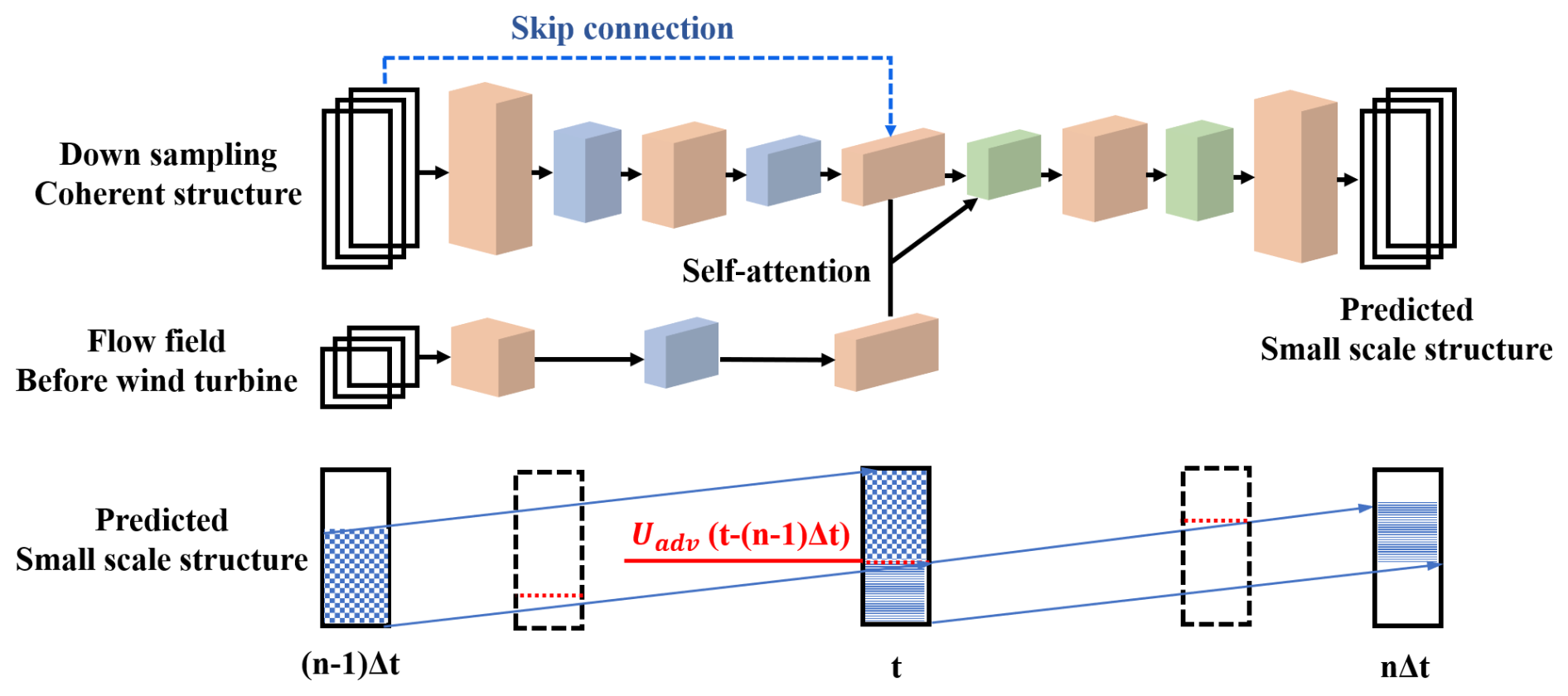
Incorporating entire snapshot sequences (i.e. the u_af(x,t_seq) input for the ${\text{CNN}}_{{\mathit{u}}^{\prime \prime }}$ model) during model training would significantly reduce efficiency and increase complexity. To address this, temporal downsampling is first applied to the snapshot sequences, substantially reducing memory requirements. The Taylor frozen hypothesis is then employed to reconstruct snapshots between sampling intervals, restoring temporal resolution while avoiding large-scale computational tasks.

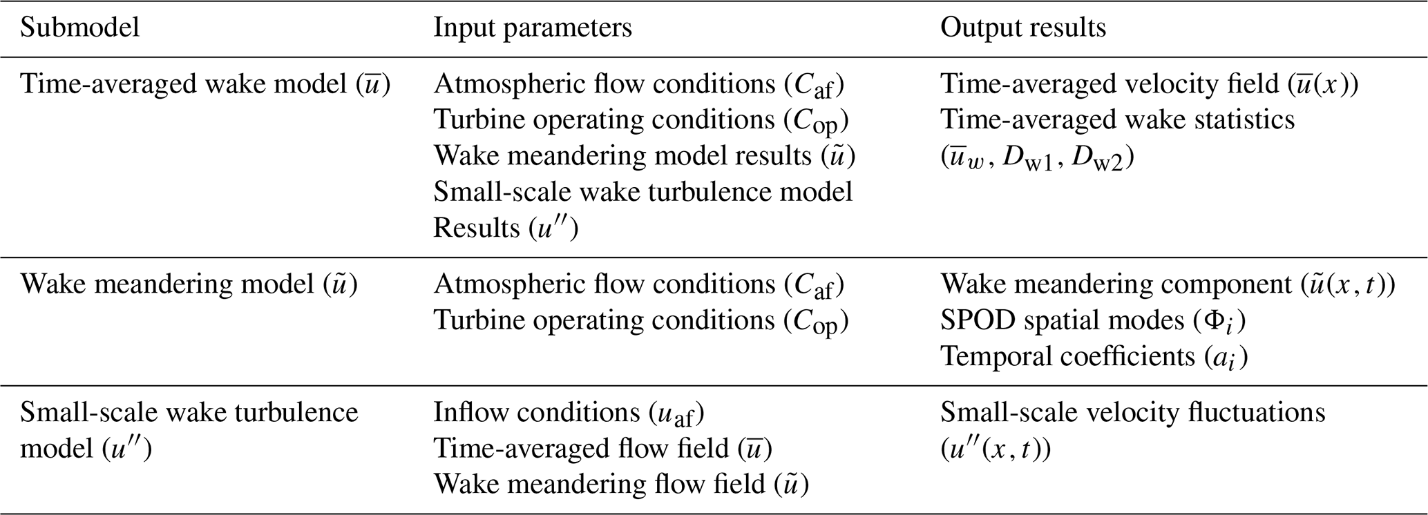
Here we list all request input parameters for the three submodels in Table 1.

Table 1 Input parameters and output results for the three submodels in the PhyWakeNet model.

2.4 Simulated cases

In this study, we employ the NREL offshore 5 MW reference wind turbine model as our baseline configuration, which was developed by Jonkman, Butterfield, and Musial (Jonkman et al., 2009). This turbine features a rotor diameter of 126 m and a cuboidal nacelle measuring 2.3 m by 2.3 m by 14.2 m.

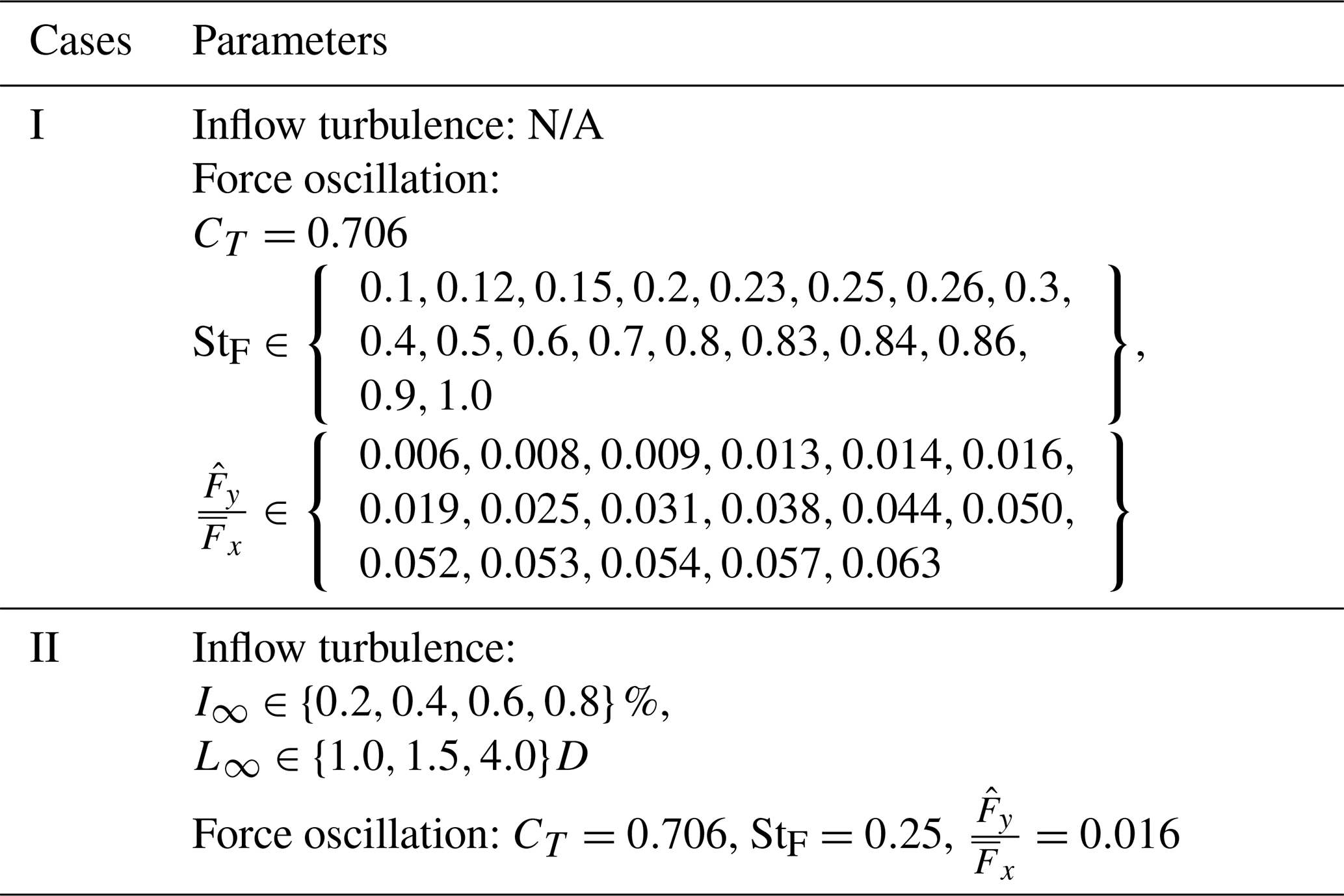
Two distinct case configurations are investigated: one with inflow turbulence and one without. The tip-speed ratio λ is set at 7, while the Reynolds number based on inflow velocity and rotor diameter reaches approximately 9.6×10⁷. The computational domain forms a cuboid measuring $\mathrm{14}D\times \mathrm{7}D\times \mathrm{7}D$ in the streamwise (x), horizontal (y), and vertical (z) directions, respectively. The rotor is positioned 3.5D downstream from the inlet, at the domain's central cross-section. A uniformly distributed inflow velocity is imposed at the inlet boundary $(x=-\mathrm{3.5}D)$, while the outlet boundary (x=10.5D) employs a Neumann condition $\left(\frac{\partial u_i}{\partial x}=\mathrm{0}\right)$. For turbulent inflow cases, velocity fluctuations generated using the synthetic turbulence technique (Mann, 1998) are superimposed onto the uniform inflow profile. Lateral boundaries implement free-slip conditions throughout the simulations.

The domain is discretized using a Cartesian grid with uniform spacing of $\mathrm{\Delta }x=D/\mathrm{20}$ in the streamwise direction and $\mathrm{\Delta }y=\mathrm{\Delta }z=D/\mathrm{20}$ within the near-wake region $(y,z\in [-\mathrm{1.5}D,\mathrm{1.5}D\left]\right)$. Grid spacing expands gradually outside this region. Comprising 281 by 141 by 141 nodes, this grid configuration has demonstrated capability for accurate predictions of velocity deficits and turbulence intensities in the turbine wake, as validated in our previous work (Li et al., 2022c). Table 2 lists all simulated cases. The specific numerical methods for generating the datasets are described in Appendix A. Except for ${\mathrm{St}}_{\mathrm{F}}=\mathrm{0.12},\mathrm{0.25},\mathrm{0.84}$, all other cases are employed for model training. The inflow turbulence was synthetically generated using the Mann turbulence generation method (Mann, 1998). The parameter L_∞ (integral length scale) represents the characteristic size of energy-containing eddies in turbulence, reflecting the average dimension of the most energetic scales in the turbulent flow, physically representing the characteristic distance travelled by an eddy before dissipation. The I_∞(turbulence intensity) is defined as the ratio of the root mean square of turbulent velocity fluctuations to the mean flow velocity, quantifying the relative magnitude of turbulent fluctuations with respect to the mean flow.

Table 2 Parameters for simulated cases.

2.5 Training of the CGAN model for generating spatial coherent modes

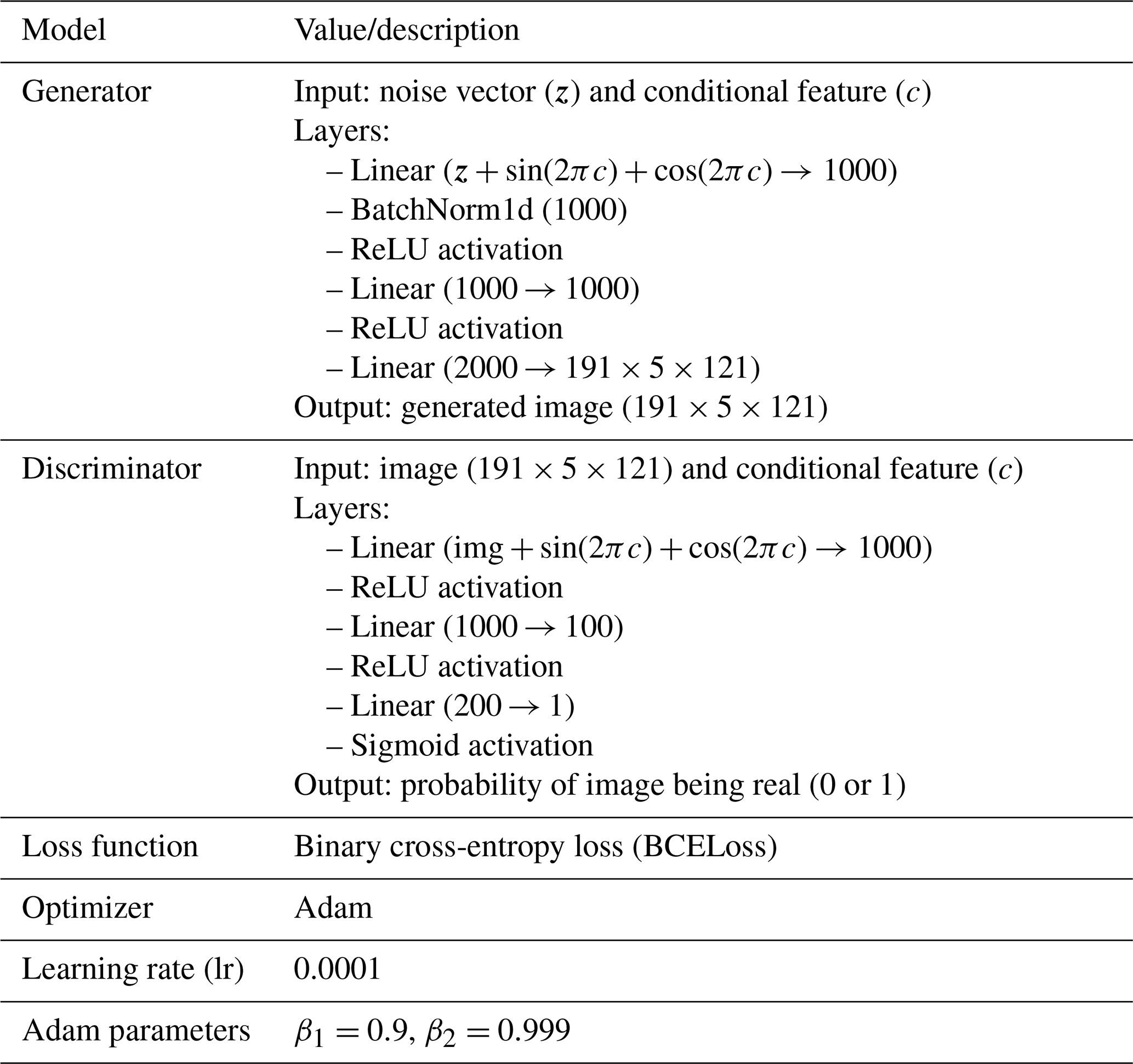
The training process involves two competing components: the discriminator learns to distinguish between authentic pairs of spatial modes with their corresponding operating conditions, while the generator attempts to produce realistic spatial modes that create data pairs indistinguishable from genuine ones. The discriminator achieves this by minimizing its classification error. The objective function is expressed as

$$\begin{array}{}\text{(33)}& \begin{array}{rl}\underset{G}{min}\underset{D}{max}V(D,G)& ={\mathbb{E}}_{{\mathbf{\Phi }}_n\sim p_{\text{data}}\left({\mathbf{\Phi }}_n\right)}\left[\log D\right({\mathbf{\Phi }}_{\mathrm{in}}\left|C_{\mathrm{n}}\right)]\\ & +\mathbb{E}\left[\log \right(\mathrm{1}-D\left(G\right({\widehat{\mathbf{\Phi }}}_{\mathrm{in}}\left|C_{\mathrm{n}}\right)\left)\right].\end{array}\end{array}$$

In this formulation, Φ_in represents an authentic sample drawn from the real data distribution p_data(Φ_in), C_n corresponds to the conditional vector, and D(Φ_in|C_n) indicates the discriminator's estimated probability that Φ_in constitutes a genuine sample under condition C_n. Since the distributions in the loss Eq. (33) remain unknown, we employ empirical loss equations following (Mirza and Osindero, 2014). The hyperparameters for both generator and discriminator are detailed in Table 3.

Training data comprise flow snapshots from LES that capture spatial modes across various operational conditions. The conditional vector C_n originates from ambient flow and turbine operation parameters. Data preprocessing involves normalization and spatial mode alignment to maintain consistent input dimensions. The generated spatial modes form 3D tensors (191 by 121 by 5) representing five dominant spatial coordinates and flow variables.

Table 3 Training details for the CGAN model.

2.6 Training of the DNN model for predicting the temporal evolution of coherent wake flows

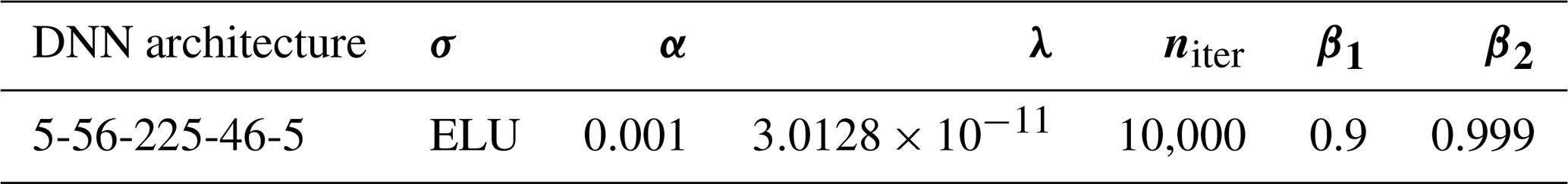
The training details of the frequency spectrum model are given as follows. The values of the hyperparameters are determined through validation errors using a systematic grid search approach. The employed hyperparameter values are presented in Table 4.

Table 4 Hyperparameters for the temporal prediction model.

The specific training details of the forcing term for the dynamic system are provided below. We generated 2000 snapshots from $t{U}_{\mathrm{\infty }}/D=\mathrm{0}$ to 10.8 through LES. For different cases, we selected varying numbers of snapshots to maintain consistent periodicity across all datasets. Our training data spans the interval from $t{U}_{\mathrm{\infty }}/D=\mathrm{0}$ to 3.6, while data beyond $t{U}_{\mathrm{\infty }}/D=\mathrm{3.6}$ serve as the test set, ensuring rigorous evaluation of the model's predictive capability on unseen data.

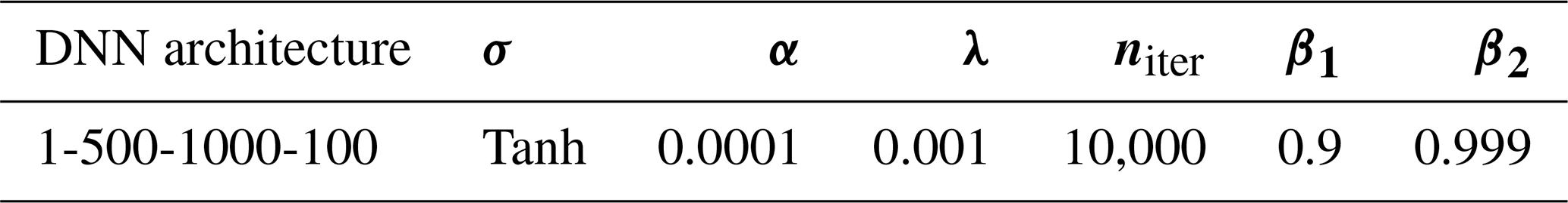
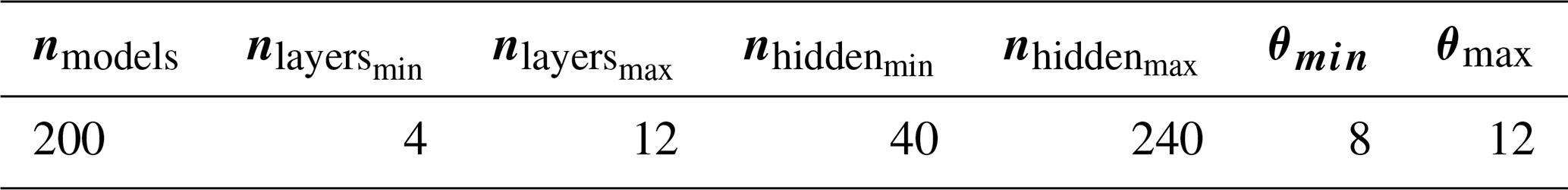
The DNN's performance critically depends on hyperparameter selection. We employed random search techniques to identify optimal hyperparameter configurations. The complete set of hyperparameters used is listed in Table 6, while the optimal set obtained through random search appears in Table 5. In both Tables 5 and 6, σ denotes the activation function, α represents the learning rate, and λ is the regularization parameter. The variable n_iter indicates the number of iterations, while β₁ and β₂ correspond to the exponential decay rates in the Adam optimization method.

Table 5 Model generation parameters for the case St=0.25.

Table 6 Optimal hyperparameters for the case St=0.25.

2.7 Training of the CNN model for predicting incoherent wake turbulence

We employ a three-dimensional convolutional neural network (3D-CNN) as our foundational architecture, as 3D-CNNs demonstrate exceptional capability in capturing complex patterns across both spatial and temporal dimensions. The model accepts a three-dimensional tensor input representing flow field data in space and time, and produces an output tensor of identical dimensions that predicts small-scale turbulence structures.

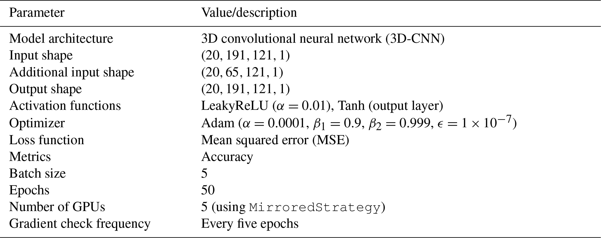
The training data originate from coarsely sampled turbulent flow fields. To implement the Taylor hypothesis, we define an advancing space line that progresses with time. Behind this space line, small-scale structures are obtained through interpolation of flow fields from subsequent time points within the coarse sampling interval. Ahead of the advancing line, small-scale structures derive from joint interpolation of flow fields from both preceding and subsequent time points within the sampling interval. Specific training parameters are detailed in Table 7.

Table 7 Training details for the 3D-CNN model.

3 Results

3.1 Tests of submodels

This section evaluates various components of the proposed model. Momentum entrainment across the wake boundary serves as the key mechanism coupling the time-averaged wake flow model with the fluctuating wake flow model. Figure 6 presents the model-predicted wake–ambient interface area A_η and the entrainment velocity v_e, compared against LES results. It is important to distinguish the different roles of the entrainment velocity as defined in Eqs. (3) and (13). Equation (13) provides the fundamental kinematic definition of the instantaneous local entrainment, representing the relative velocity component normal to the fluctuating wake boundary. This definition captures the detailed, time-dependent mixing physics at the interface. In contrast, Eq. (3) is an analytical parameterization designed for the time-averaged conservation equations (Eq. 2). In this context, the entrainment coefficient E serves as a critical closure term. It bridges the gap between the detailed unresolved velocity fluctuations and boundary motions (fundamentally described by Eq. 17) and the macro-scale mean flow properties. By incorporating the coefficient E, the time-averaged model can effectively account for the integrated effects of both coherent wake meandering and small-scale turbulence on wake recovery without needing to explicitly resolve the high-frequency dynamics of the wake interface. Overall, good agreement is observed, especially the different streamwise evolutions under different force oscillating frequencies, although the model predictions are slightly lower. This discrepancy is considered acceptable, as the small-scale curled structures along the interface are challenging to capture accurately.

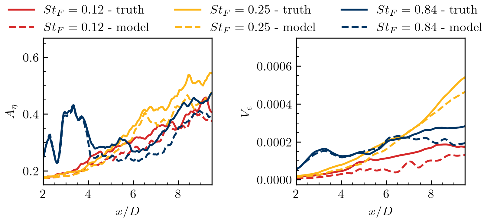
Figure 6 Comparison of the wake–ambient interface area A_η and entrainment velocity V_e correspond to three different aerodynamic force disturbance characteristic frequencies of St_F=0.12, St_F=0.25, and St_F=0.84.

The wake–ambient interface area (A_η) and entrainment velocity (v_e) are compared against the LES results in Fig. 6. Upper (η_u) and lower (η_l) wake boundaries are established as the iso-surface of the streamwise velocity deficit (Δu). The area (A_η) is then integrated based on the identified wake boundaries. The entrainment velocity (v_e) is approximated by Eq. (26), and the transverse wake centre y_c is determined by using the transverse coordinates of the upper (η_u) and lower (η_l) boundaries, as described in Eq. (18).

This work is based on the fundamental assumption that the coherent flow component is predictable. To verify this assumption, we evaluate the model's performance in predicting leading SPOD modes for three characteristic aerodynamic force oscillation frequencies (St=0.12, 0.25, and 0.84) in Fig. 7. As seen, our model demonstrates excellent performance across most cases, except for low-frequency conditions where coherent structures are less distinct. The model particularly excels at capturing the hub vortex formation, which produces a characteristic meandering pattern near the nacelle centreline in the highest frequency test case (St=0.84). For the intermediate frequency case (St=0.25), the simulation reveals a gradual downstream expansion of the meandering pattern. Conversely, the low-frequency case (St=0.12) exhibits minimal spatial growth of the meandering pattern, a behaviour that the model reproduces accurately. Overall, the results confirm the model's capability in predicting coherent wake dynamics under aerodynamic force oscillations in terms of (1) global flow pattern morphology, (2) downstream evolution characteristics, and (3) systematic variation with oscillation frequency.

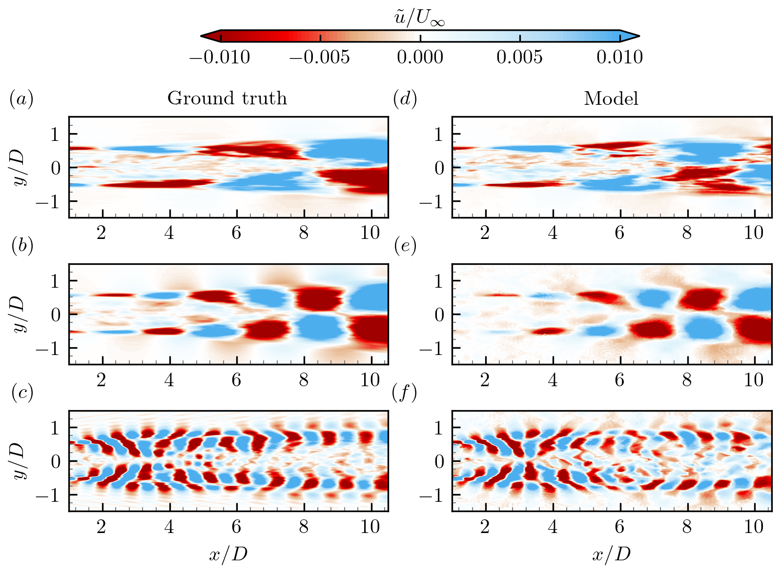
Figure 7 Comparison of the first SPOD mode for the test cases with St_F=0.12 (a, d), St_F=0.25 (b, e), and St_F=0.84 (c, f), with (a–c) and (d–f) showing the results predicted by large-eddy simulation and the proposed model, respectively.

The capability of the proposed model in predicting the energy spectra of SPOD modes is examined in Fig. 8, comparing three configurations: (1) large-scale structures reconstructed from the first two modal orders without the incoherent wake flow model, (2) large-scale structures combined with reconstructed small-scale turbulence using the incoherent wake flow model, and (3) reference LES results. The spectrum exhibits distinct peaks at St=0.25 and 0.84 in Figures 8b and c, respectively, corresponding to the aerodynamic force oscillation frequency and dominant coherent flow structures. All three cases show an inertial subrange following the $-\mathrm{5}/\mathrm{3}$ power law. While the dominant peak frequency is well captured by the model without the incoherent wake flow model, the energy densities at other frequencies are significantly underpredicted and fail to exhibit the $-\mathrm{5}/\mathrm{3}$ scaling. With the inclusion of the incoherent wake flow model, the reconstructed flow field's energy spectra show excellent agreement with reference LES data across all frequencies in Fig. 8, extending even beyond the coarse sampling frequency (indicated by the grey line) used as input for the small-scale model. This demonstrates the model's remarkable generative capabilities. Furthermore, for the St=0.12 case, the energy density at the corresponding frequency is less pronounced compared to the other two cases. In contrast, the St=0.84 case reveals two harmonics of the fundamental frequency. The proposed model successfully captures these spectral variations with respect to aerodynamic force oscillation frequency.

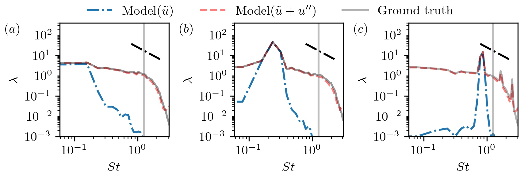
Figure 8 A comparison of the energy spectra of the leading SPOD mode corresponds to the three different aerodynamic force disturbance characteristic frequencies of St_F=0.12 (a), St_F=0.25 (b), and St_F=0.84 (c). In the figure, the dashed black line represents the $k^{-\mathrm{5}/\mathrm{3}}$ law, while the solid grey line indicates the corresponding dimensionless frequency after temporal downsampling in the time domain. The dashed red lines and dash-dot blue lines represent the results with and without the inclusion of the incoherent wake flow model.

At last, the performance of the wake flow model for small-scale fluctuations is tested. Figure 9 shows the comparison of the model-predicted small-scale velocity fluctuations with the LES results. Although the amplitudes of velocity fluctuations are somewhat underpredicted, two critical characteristics are well captured. They include (1) the development of small scales, which initiate around the ambient–wake interface, grow in amplitude, and expand in the radial direction as travelling downstream; and (2) the impacts of wake meandering on small-scale fluctuations, which follow the meandering pattern and are significantly amplified by the meandering motion.

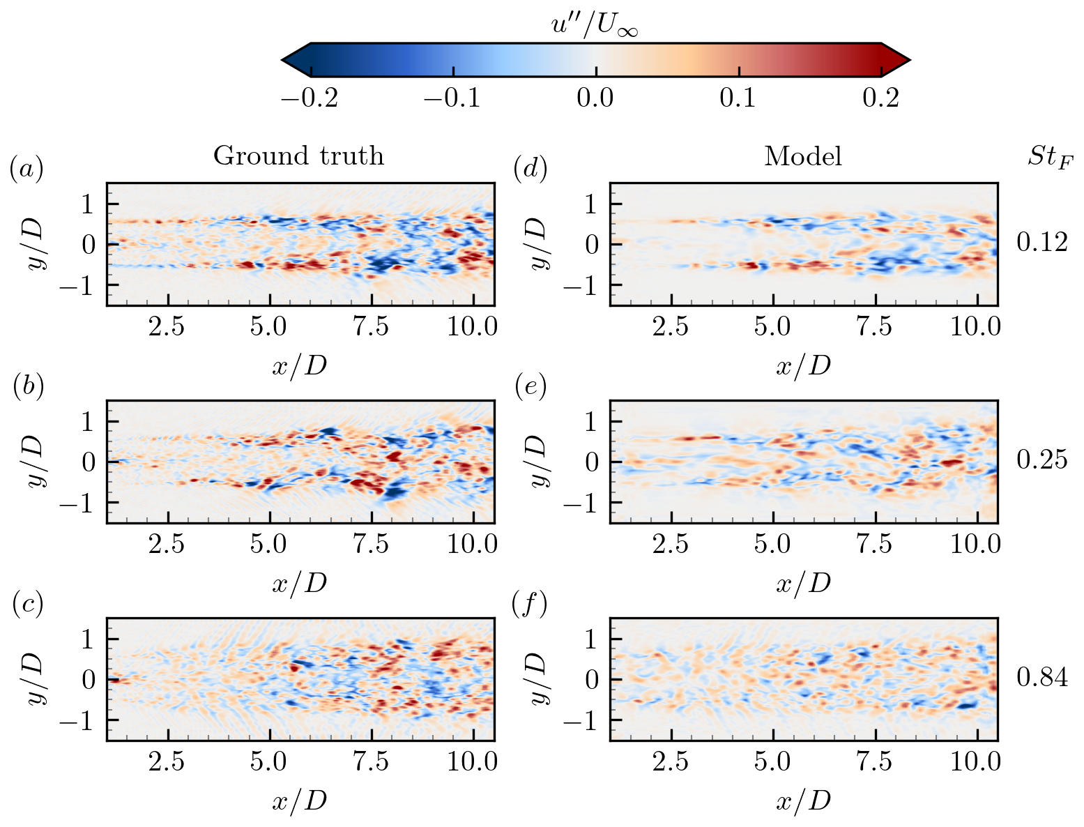
Figure 9 Small-scale velocity fluctuations obtained from LES (a–e) and the proposed model (f–j) at the same instants. The contour is coloured by instantaneous streamwise velocity. The three rows from top to bottom correspond to three aerodynamic force oscillation frequencies St=0.12, St=0.25, and St=0.84, respectively.

To further provide a more vivid and interpretable description of how the CNN processes flow features, a SHapley Additive exPlanations (SHAP) analysis is incorporated to explain the model’s internal decision-making. SHAP offers a unified framework for quantifying the contribution of each input variable to the predicted small-scale fluctuations, thereby revealing which flow features the CNN relies on most. In this work, the SHAP analysis is carried out at two physically distinct locations: position A at the wake centreline and position B in the shear layer.

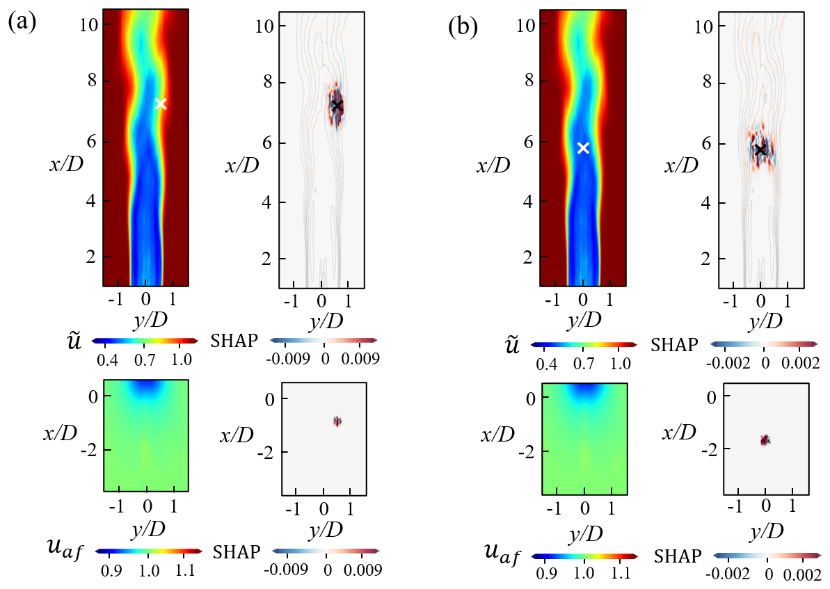
Figure 10 Local SHAP analysis for predictions at two distinct target locations. The figure provides the local SHAP explanations for the model's predictions of one test sample at two different target locations: (a) position A, located at the wake centreline; and (b) position B, situated within the shear layer. For each subfigure, the top row displays the original main input map ($\stackrel{\mathrm{‾}}{\mathit{u}}\left(\mathit{x}\right)+\stackrel{\mathrm{̃}}{\mathit{u}}(\mathit{x},t)$) and its feature contributions (SHAP values: red for positive, blue for negative) to the respective target point (marked X). The bottom row shows the u_af (velocity field of the ambient flow from the upstream measurement) and its corresponding SHAP contributions. This dual visualization allows for the identification and comparison of specific spatial and parametric features most responsible for the model's output at the two explained locations.

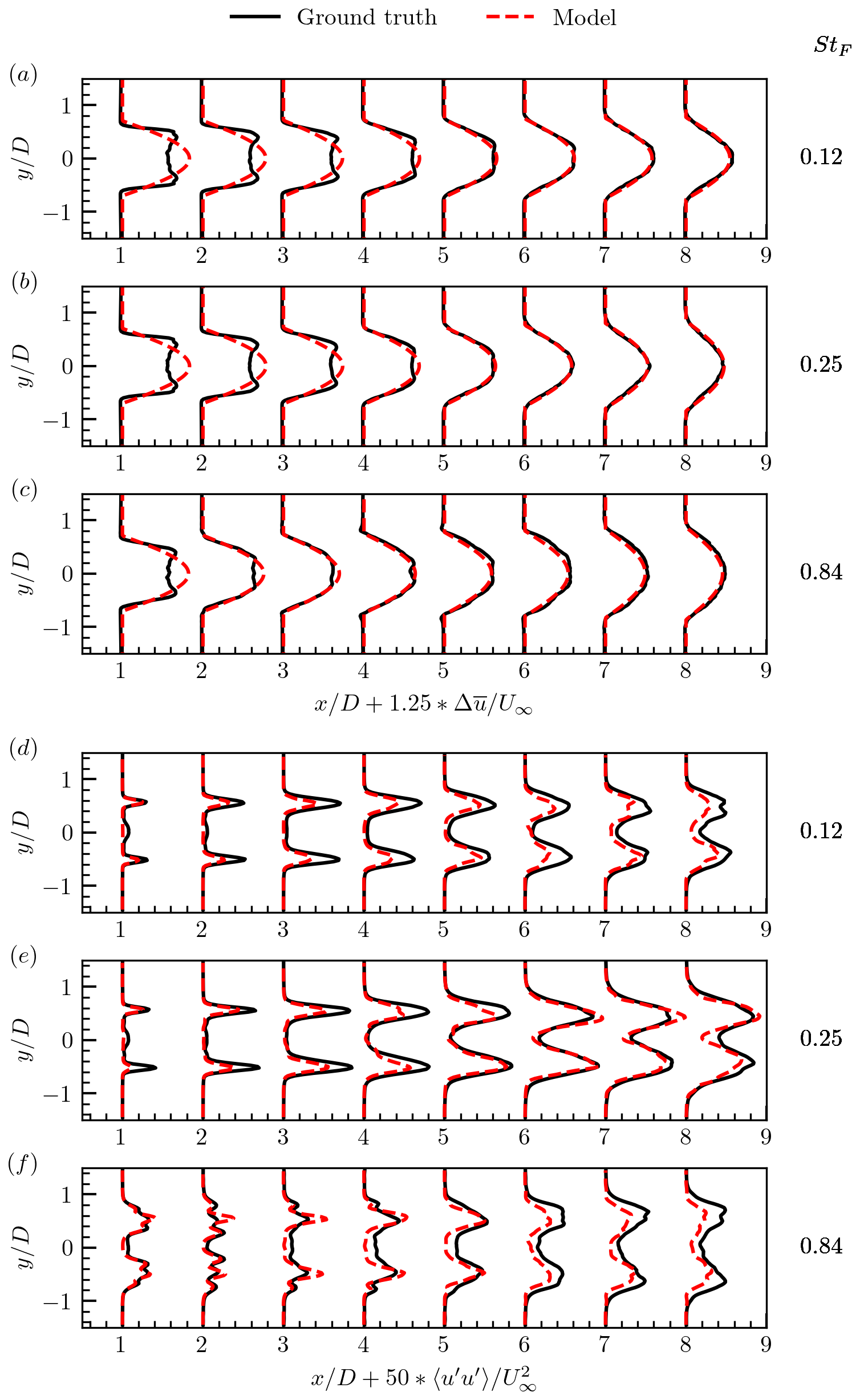
Figure 11 Time-averaged streamwise velocity deficit ($\mathrm{\Delta }\stackrel{\mathrm{‾}}{u}$, (a–c)) and variance of streamwise velocity fluctuation ($\langle u^{\prime }{u}^{\prime }\rangle$, d–f) profiles at various wind turbine downwind positions for three aerodynamic force oscillation frequencies (a, d) St=0.12, (b, e) St=0.25, and (c, f) St=0.84. Solid black lines: reference LES results; dashed lines: model predictions for red $\mathrm{\Delta }\stackrel{\mathrm{‾}}{u}$ and blue $\langle u^{\prime }{u}^{\prime }\rangle$. The normalized velocity deficit and variance are multiplied by constants C₁=1.25 and C₂=50, respectively, for better visual comparison of the relative spatial distributions in a single plot.

As shown in the SHAP contribution map (Fig. 10), the model’s feature importance is significantly different at the two positions. For position A, which is characterized by a low intensity of small-scale turbulence, the model predominantly attributes feature importance to a square-like region centred around the target point. This large, block-shaped contribution suggests that small-scale fluctuations are not governed by local features but by the overall state of the wake interior. Since velocity gradients are weak near the centreline, small-scale turbulence is mainly supplied through inward transport and the redistribution of fluctuations generated in the shear layers. Conversely, at position B, a region of intense small-scale structural activity and strong velocity gradients, the dominant contributions come from a narrow, elongated strip aligned primarily in the streamwise direction along the wake boundary. These elongated strip patterns correspond to the footprints of shear-layer roll-up and subsequent distortion by wake meandering, which act as the primary source of small-scale turbulence generation in this region.

A shared characteristic across both analyses is the primary contribution regions of the inflow turbulence (u_af) fields, which are relatively localized. Notably, the inflow snapshots involved in the prediction are direct samples from previous time steps, mapped to the inflow boundary using Taylor’s frozen turbulence hypothesis. Besides, the primary contribution regions are straight aligned, with the streamline passing through the target location. This indicates that the influence of inflow turbulence on the target location is governed primarily by streamwise convective transport, consistent with Taylor’s frozen turbulence assumption.

3.2 Time-averaged wake flow statistics

The section examines the time-averaged flow statistics predicted by the model. The quantitative evaluation of the proposed model's prediction of time-averaged wake statistics is presented in Fig. 11. We first examine the time-averaged velocity deficits $\mathrm{\Delta }\stackrel{\mathrm{‾}}{u}$. Although discrepancies exist in the shape of the velocity deficit in the near-wake region, the proposed model demonstrates strong predictive capabilities in the far-wake region, with predicted curves closely matching the reference profiles. The model accurately predicts differences in wake development for various aerodynamic force oscillations. Specifically, it captures the faster wind speed recovery observed for the two higher force oscillation frequencies (St=0.25 and 0.84). The overall agreement with reference profiles confirms the model's effectiveness in capturing the downwind wind speed recovery. This success stems from properly accounting for enhanced entrainment due to both coherent flow patterns and small-scale velocity fluctuations.

We first compare the model predictions of the mean streamwise velocity averaged over the wake's cross-section, and the minor and major axis diameters of the wake's cross-section with the LES results. As seen in Fig. 12, the proposed model accurately captures the impacts of aerodynamic force oscillation frequencies on mean streamwise velocity and wake diameters. The wake recovers faster at the frequencies St_F=0.25, 0.84 compared with St_F=0.12. The streamwise velocity in the wake with St_F=0.84 is higher than the other two at 2D  3D turbine downstream locations. The wake flow with St_F=0.25, on the other hand, starts its faster recovery at around 5D turbine downstream because of the onset of wake meandering.

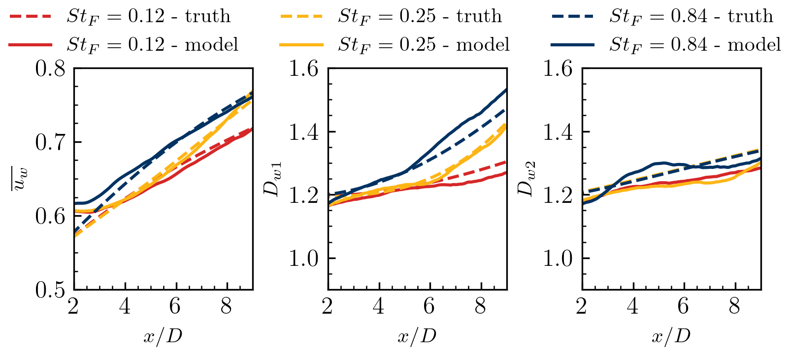
Figure 12 Comparison of the mean streamwise wake velocity ${\stackrel{\mathrm{‾}}{u}}_{\mathrm{w}}$, the major axis diameter D_w1, and the minor axis diameter correspond to three different aerodynamic force disturbance characteristic frequencies of St_F=0.12, St_F=0.25, and St_F=0.84.

We then examine the variance of the streamwise velocity fluctuations ($\langle u^{\prime }{u}^{\prime }\rangle$) predicted by the proposed model. Overall good agreement with the reference data is observed, particularly for the case with St=0.25 where significant wake meandering occurs. The model demonstrates particular accuracy in predicting (1) the locations of high-intensity $\langle u^{\prime }{u}^{\prime }\rangle$ variance of streamwise velocity fluctuations, which primarily occur near the blade tips; and (2) the overall magnitude of $\langle u^{\prime }{u}^{\prime }\rangle$ fluctuations. For cases with St=0.12 and 0.84, where the wake lacks dominant coherent flow structures, the agreement with reference $\langle u^{\prime }{u}^{\prime }\rangle$ data remains acceptable, although with larger discrepancies compared to the St=0.25 case. Overall, the model demonstrates strong capabilities in predicting basic wake flow statistics, including both the mean velocity deficit and streamwise velocity fluctuation variance. The following analysis focuses on evaluating the model's performance in predicting wake meandering statistics.

3.3 Instantaneous wake flows

This section demonstrates the capability of the model in predicting instantaneous wake flows. We first compare the model-predicted instantaneous streamwise velocity fields against LES results in Fig. 13. The proposed model demonstrates strong agreement in capturing the onset of wake meandering, the large-scale meandering patterns across all tested locations, and the distinct wake behaviour for different aerodynamic force oscillation frequencies. Quantitatively, the onset of wake meandering is identified by the location where σ_yc (standard deviation of wake centre) exceeds 0.05D. The proposed model predicts this onset at $x/D\approx \mathrm{5.8}$, which agrees well with the LES result of $x/D\approx \mathrm{5.4}$ at case St_F=0.25, showing a deviation of only 7.5 %. The detail of onset location prediction performance and relative error can be viewed in Fig. 14. The model successfully reproduces small-scale flow structures that predominantly emerge along the wake boundary and surround the large-scale coherent structures. One limitation concerns the nacelle-induced flow fluctuations – that the near-wake centreline features are not captured. This is expected given the cosine-shaped velocity deficit assumption, and the exclusion of nacelle effects and initial wake development physics in the model.

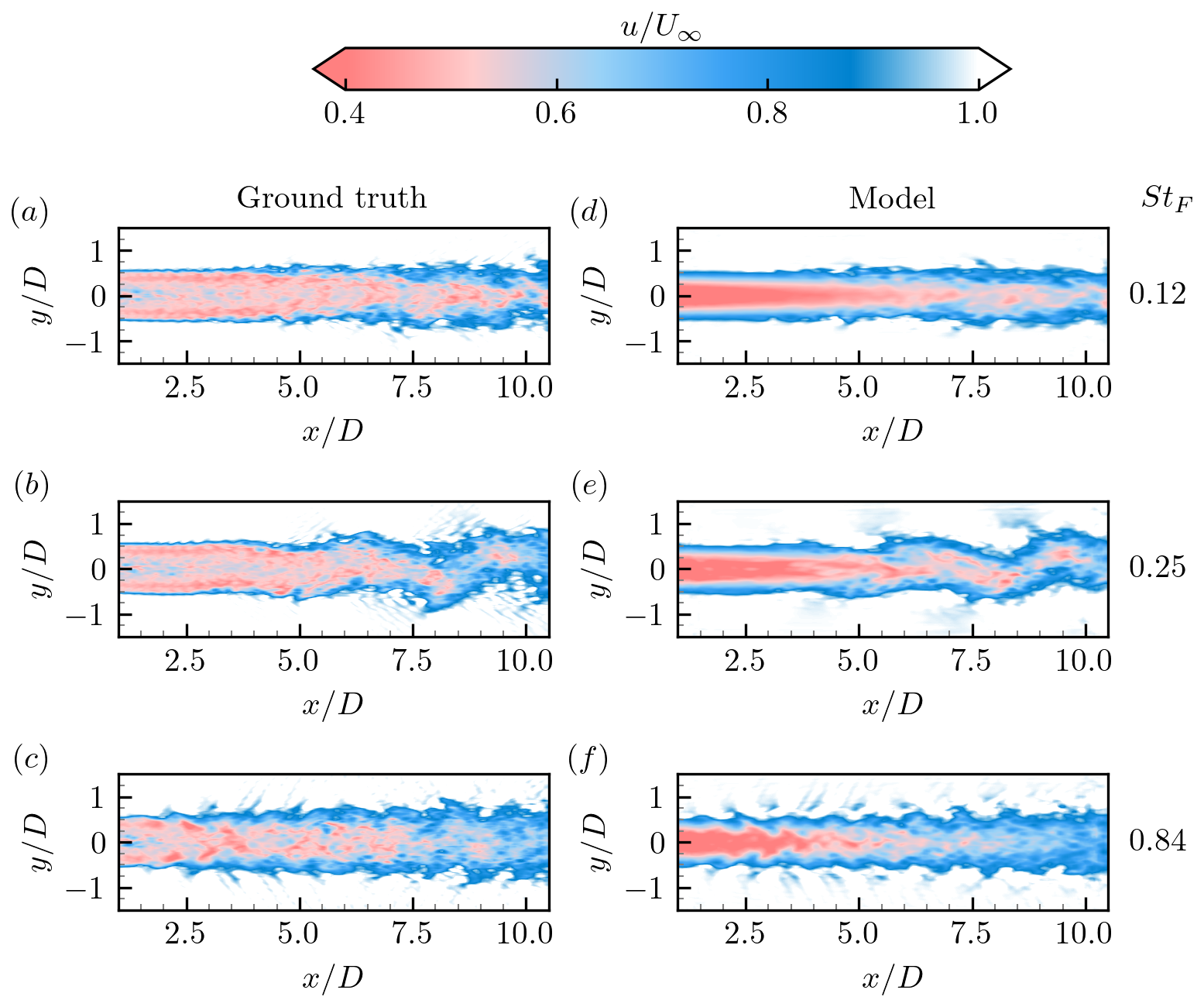
Figure 13 Instantaneous flow fields obtained from LES (a–c) and the proposed model (d–f) at the same instants. The contour is coloured by instantaneous streamwise velocity. The three rows from top to bottom correspond to three aerodynamic force oscillation frequencies St=0.12, St=0.25, and St=0.84, respectively.

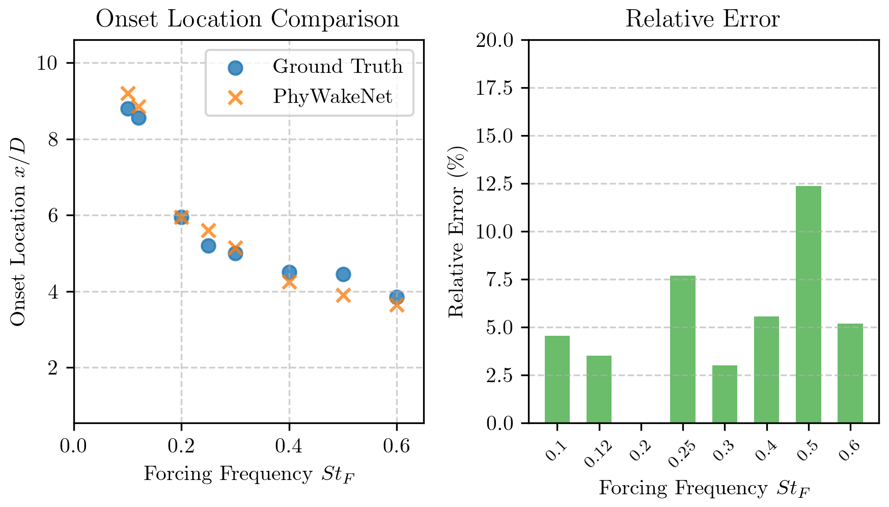
Figure 14 Comparison of the wake onset location predicted by PhyWakeNet and LES: (a) onset location $x/D$ as a function of the forcing frequency St; (b) relative error of the prediction for each case, where the dotted red line indicates the mean relative error across all strongly meandering behaviour cases (including both training and testing sets).

The amplitude of wake meandering σ_y, defined as the standard deviation of instantaneous wake centre positions in the spanwise direction, is presented in Fig. 15 for downstream locations $x/D=\mathrm{5}$ and 10. In this figure, the red lines represent the predictions of the proposed model, while the grey lines correspond to the LES reference data. The proposed model accurately predicts the variation of σ_y with respect to aerodynamic force oscillation frequency (St) and atmospheric turbulence conditions. At $x/D=\mathrm{5}$, σ_y exhibits a maximum in the frequency range $\mathrm{0.4}\le \mathrm{St}\le \mathrm{0.6}$, decreasing for both higher and lower frequencies. While the model captures this trend well, it shows slight overestimations of σ_y within this frequency range. Further downstream, at $x/D=\mathrm{10}$, the wake meandering amplitude σ_y displays a pronounced peak near St=0.3, with rapid decay at both higher and lower frequencies – a characteristic that the model reproduces with good fidelity. The quantitative agreement between the model and LES results is evaluated using the normalized root mean square error (NRMSE), defined as

$$\begin{array}{}\text{(34)}& \mathrm{\text{NRMSE}}={\displaystyle \frac{\mathrm{1}}{{\stackrel{\mathrm{‾}}{y}}_{\text{ground truth},i}}}\sqrt{{\displaystyle \frac{\mathrm{1}}{N}}\sum _{i=\mathrm{1}}^N(y_{\text{model},i}-y_{\text{ground truth},i}{)}^{\mathrm{2}}}.\end{array}$$

Table 8 Quantitative comparison of the relative profile error (NRMSE, %) for streamwise velocity (u) and variance of streamwise velocity fluctuations ($\langle u^{\prime }{u}^{\prime }\rangle$) at different streamwise locations and oscillation frequencies.

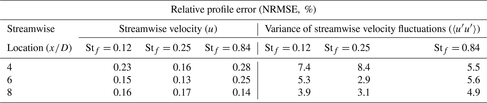
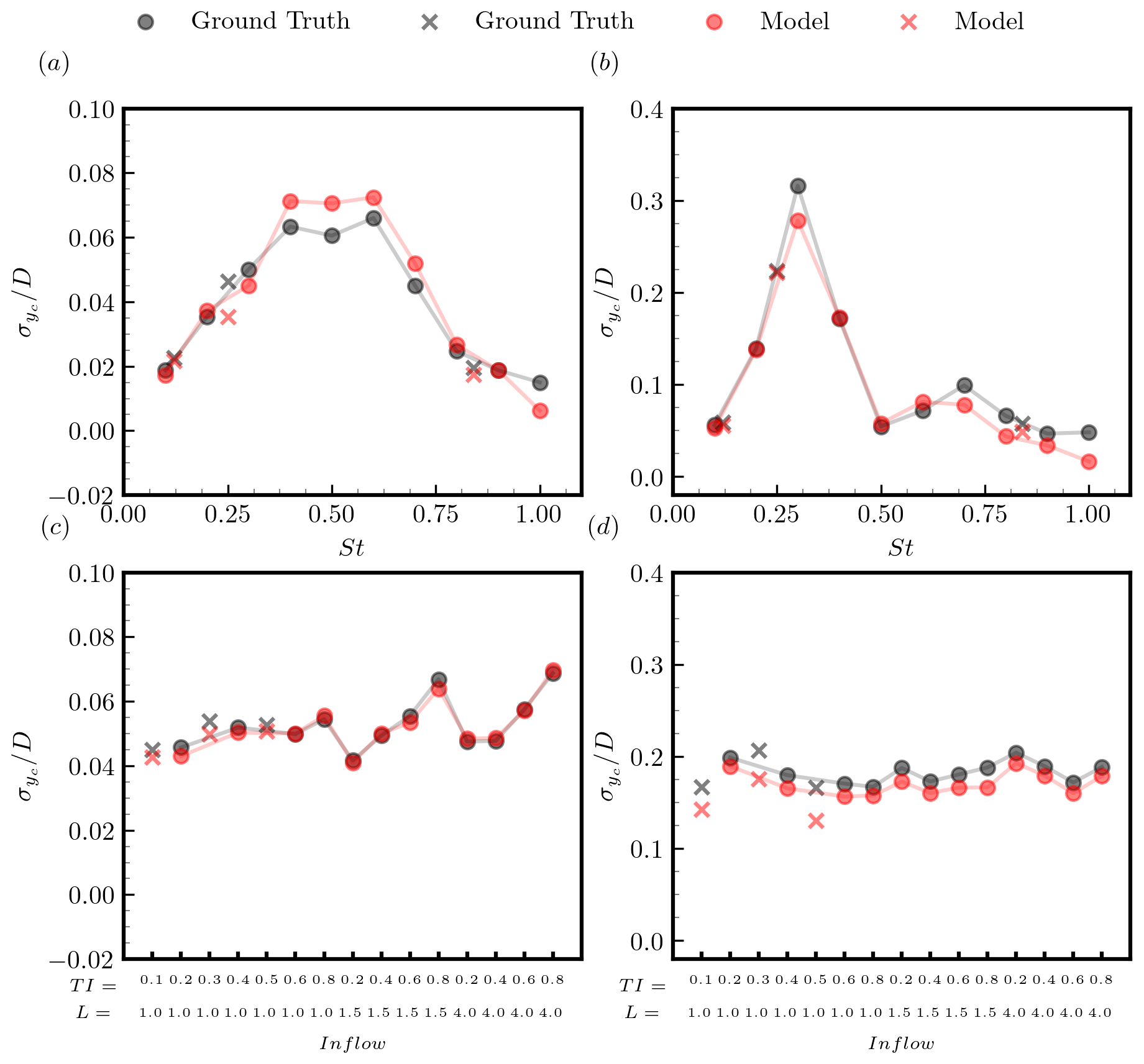
Figure 15 Comparison of actual and model-predicted wake centre fluctuation amplitudes under varying aerodynamic force oscillation frequencies (a, b) and varying turbulent inflows (c, d). The subplots (a, c) show the comparison at a streamwise position of $x/D=\mathrm{5}$, while the subplots (b, d) show the comparison at a streamwise position of $x/D=\mathrm{10}$. The 13 frequencies in (a, b) are 0.1, 0.12, 0.2, 0.25, 0.3, 0.4, 0.5, 0.6, 0.7, 0.8, 0.84, 0.9, and 1.0. The 12 inflows in (c, d) are the results of three turbulent integral length scales and four turbulent intensities. The crosses represent the unseen cases.

For $x/D=\mathrm{5}$ and 10, the relative error in σ_y (PhyWakeNet vs. LES) is <15 % across all St_F. The analysis of inflow turbulence effects reveals that: (1) at $x/D=\mathrm{5}$, the wake meandering amplitude is higher for higher inflow turbulence intensity; (2) at $x/D=\mathrm{10}$, the sensitivity to inflow turbulence conditions diminishes significantly.

In active wake control applications, precise prediction of wake positions is essential. Figure 16 evaluates the model's performance in this regard by analysing temporal variations of both spanwise wake centre positions (y_c) and wake centreline velocity deficits (Δu_c) at the 10D downstream location. For the high-frequency forcing case (St=0.84), the model exhibits a noticeable degradation in predicting the wake velocity deficit and profile shape, while the prediction of the wake centre position y_c remains reasonably accurate. This behaviour should not be interpreted as a failure of the model but rather as a manifestation of the underlying scale-dependent predictability of wake dynamics. In the present framework, it is assumed that the dominant large-scale quasi-coherent wake structures are predictable, whereas the small-scale turbulent motions are inherently stochastic and therefore not fully predictable. At low and intermediate forcing frequencies, the wake response is largely governed by organized large-scale structures, for which the model demonstrates strong predictive capability. In contrast, at St=0.84, the wake dynamics are increasingly dominated by small-scale turbulent motions induced by rapid aerodynamic fluctuations. The intensified turbulent mixing accelerates the breakdown of coherent structures and enhances wake recovery, resulting in a highly distorted velocity field. Since a substantial portion of the wake deficit in this case originates from small-scale contributions, the reduced prediction accuracy in velocity deficit is physically expected. Nevertheless, the model retains its ability to capture the large-scale wake deflection, as evidenced by the satisfactory prediction of y_c. The proposed model demonstrates strong predictive capability, accurately capturing both long-term trends and short-term fluctuations in the wake behaviour. While the agreement with reference data is generally good for both quantities, the predictions for y_c show better correspondence than those for Δu_c. This performance discrepancy arises partly from the underlying assumptions of the modelling framework: the time-averaged wake velocity deficit distribution is imposed a priori (via a cosine-shaped profile assumption) rather than dynamically simulated. By adopting this prescribed cosine profile, the model oversimplifies the actual time-averaged wake structure, which in turn compromises the accuracy of Δu_c predictions – since the centreline velocity deficit is more sensitive to deviations from the true time-averaged wake shape compared to the wake centre position. This sensitivity arises because the centreline velocity deficit represents a local maximum of the wake profile, making it highly dependent on the assumed functional form. In contrast, the wake centre position is primarily determined by the first moment of the velocity field and is thus less sensitive to the detailed profile shape.

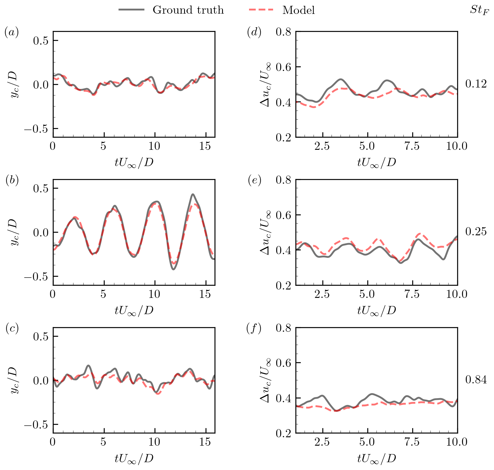
Figure 16 Comparison of temporal variations of spanwise wake centre positions (y_c, a–c) and wake centreline velocity deficits (Δu_c, d–f) at the 10D downstream location. From top to bottom are three cases with motion frequencies of St_F=0.12, St_F=0.25, and St_F=0.84, respectively. The solid lines and the dashed lines represent the results of large-eddy simulation and the proposed model, respectively.

4 Conclusions

We proposed a physics-integrated GAN-CNN wake model (PhyWakeNet) for predicting the dynamics of wind turbine wakes under aerodynamic force oscillations. The PhyWakeNet model integrates three interconnected submodels: the time-averaged wake model, the wake meandering model, and the model for small-scale turbulence.

The time-averaged wake model is derived from the fundamental mass and momentum conservation principles, with its entrainment parameter dynamically determined based on the other two submodels. For wake meandering prediction, the model employs a spatiotemporal decomposition approach where the spatial modes are reconstructed through a combination of spectral proper orthogonal decomposition (SPOD) and conditional generative adversarial network (CGAN). Computational efficiency is maintained by retaining only the first five SPOD modes. Temporal evolution is captured through a dynamic system model enhanced by a deep neural network (DNN)-derived forcing term. The small-scale turbulence is generated by a convolutional neural network (CNN) that processes three key inputs: time-averaged wake field, wake meandering, and inflow turbulence. This comprehensive approach enables the model to capture a broad spectrum of wake dynamics.

Validation studies across various aerodynamic force oscillations and inflow turbulence conditions demonstrate the model's capabilities in capturing both the time-averaged and dynamic features of wind turbine wakes. The prediction error of PhyWakeNet for average velocity deficit is under 1 %, while velocity fluctuation and meandering amplitude errors are within 10 % and 15 %. In cases with significant meandering behaviour, the error in predicting the meandering onset position is less than 12.5 %. These results confirm the model's reliability in capturing both the mean flow and dynamic wake motion. The results show that the PhyWakeNet model accurately reproduces frequency-dependent variations in wake characteristics, outperforming existing engineering wake models in several aspects. Beyond predicting velocity deficits – a standard capability of traditional models – it successfully captures turbulence intensity distributions and the fluctuating wake features, including instantaneous wake positions and velocity deficits.

One major limitation of the learned model is that it was solely trained using the NREL 5 MW wind turbine with aerodynamic force oscillations in one particular direction, although the proposed framework is applicable to cases with different forms of force oscillations or their combinations, and other turbine designs. For engineering applications with known active wake mixing strategies (i.e. known force oscillations), a case-by-case model can be developed. To develop a generally applicable model using the proposed framework, one straightforward way is to build a dataset covering a wide range of forcing parameters. This, however, is computationally prohibitive considering the large parameter spaces of both atmospheric conditions and turbine operational conditions to be considered. Incorporating physics in the model learning is an alternative, promising solution either for a generally applicable model or a model for a specific form of force oscillations.

Appendix A: Numerical methods

The training datasets are generated using the large-eddy simulation module of the Virtual Flow Simulator (VFS-Wind) code (Yang et al., 2015; Yang and Sotiropoulos, 2018; Santoni et al., 2023). The flow physics is governed by the filtered incompressible Navier–Stokes equations:

$$\begin{array}{ll}{\displaystyle }& {\displaystyle \frac{\partial u_j}{\partial x_j}}=\mathrm{0}\\ \text{(A1)}& {\displaystyle }& {\displaystyle \frac{\partial u_i}{\partial t}}+{\displaystyle \frac{\partial u_i{u}_j}{\partial x_j}}=-{\displaystyle \frac{\mathrm{1}}{\mathit{\rho }}}{\displaystyle \frac{\partial p}{\partial x_i}}+{\displaystyle \frac{\partial }{\partial x_j}}\left(\left(\mathit{\nu }+{\mathit{\nu }}_t\right){\displaystyle \frac{\partial u_i}{\partial x_j}}\right)+f_i,\end{array}$$

where $i,j=\mathrm{1},\mathrm{2},\mathrm{3}$ denote spatial indices, u represents the velocity field, p is the pressure, ν indicates the kinematic viscosity, and ν_t stands for the eddy viscosity modelled through the Smagorinsky model with dynamically determined coefficients. The body force term f_i (per unit mass) originates from the actuator surface model, which captures both turbine blades and nacelle effects. Unlike the commonly used actuator line model, the actuator surface method explicitly incorporates blade geometry features, particularly the chord distribution along the spanwise direction, while also resolving nacelle geometry (Yang and Sotiropoulos, 2018). Force and torque conservation during information transfer between the actuator surface grid and background flow solver grid is maintained through a smoothed discrete delta function approach (Yang et al., 2009) using just 3 to 5 grid cells.

Spatial discretization employs a second-order central difference scheme, coupled with temporal advancement via a second-order fractional step method (Ge and Sotiropoulos, 2007). The momentum equation solution utilizes a matrix-free Newton–Krylov approach (Knoll and Keyes, 2004), while the pressure Poisson equation is solved through the generalized minimal residual (GMRES) method accelerated by algebraic multi-grid techniques.

Appendix B: Application to an in-line two-turbine array

B1 Case setup

In this appendix, we illustrate the application of the proposed model to predict wake flows in an in-line two-turbine array. A schematic of the considered scenario is shown in Fig. B1. As seen, in this scenario, the oscillating aerodynamic forces are only applied on the upstream wind turbine with the downstream wind turbine operating in the conventional way. Such configuration is set under the consideration that applying active wake mixing control only at the upstream turbine is effective for a turbine array, which is inspired by the observation that the meandering of a downstream wind turbine essentially follows that from the incoming wake. In the simulated cases, the Strouhal number of the aerodynamic force oscillations of the upstream wind turbine is fixed at St_F=0.25, with the forcing amplitude $\frac{{\widehat{F}}_y}{{\stackrel{\mathrm{‾}}{F}}_x}=\mathrm{0.016}$. Three streamwise turbine spacings are considered, i.e. $\mathrm{\Delta }S/D=\mathrm{4},\mathrm{5}$, and 6. The data from the case with $\mathrm{\Delta }S/D=\mathrm{4}$ and 6 and the original one-turbine cases' data are employed for model training, while the data from the one with $\mathrm{\Delta }S/D=\mathrm{5}$ are for testing.

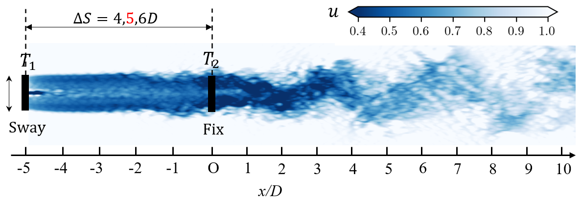
Figure B1 Schematic of the in-line two-turbine array case. The upstream turbine (T₁) undergoes periodic swaying at St_F=0.25, while the downstream turbine (T₂) remains fixed at a distance of $\mathrm{\Delta }S=\mathrm{4},\mathrm{5}$, or 6D. The background contours represent the instantaneous velocity field u, highlighting the turbulent wake interaction between the two turbines.

B2 Model setup

The adjustments of the proposed model for its application to turbine arrays are listed as follows.

• For the time-averaged wake model, the initial streamwise velocity deficit and wake widths at 1D downstream of the T₂ turbine are computed using the incoming velocity and wake widths at 0.5D upstream of the T₂ turbine, which is given by the time-averaged wake prediction of the upstream T₁ wind turbine.

• For the coherent wake component, the coherent motions predicted in the upstream T₁ turbine's wake are directly employed for the T₂ turbine. With the energy extraction, the T₂ turbine does add perturbations to the coherent flow structures. Away from the near-wake region of T₂, the overall patterns, however, remain approximately the same in the far-wake region. This is the reason why the coherent motion in T₁'s wake without T₂ are directly employed. With more turbines added at downstream locations, such simplifications will fail. Modelling the interaction between the incoming coherent structures and those generated in the wake is challenging itself, and worth being carried out in another work.

• The small-scale model is retrained by adding the data pairs, i.e. the inflow (i.e. turbulence intensity and integral length scale at 0.5D upstream of the T₂ turbine) and the predicted coherent motion as the input, and the small-scale turbulence in the T₂'s wake as the output from the 4D and 6D cases, to the single-turbine cases' data.

• Modelling wake superposition is particularly challenging for dynamic wake models, as one has to take care of both the time-averaged and coherent components. A fairly simplified approach is taken in the present work. In this approach, the wake superposition is accounted for using the inflow velocity deficit and wake width from the T₁'s wake to determine those of the T₂'s wake. The cases considered in this work are under full wake conditions with T₂ directly in the wake of T₁. For partial wake conditions, asymmetry can be introduced to the initial wake width of T₂.

B3 Results

The time-averaged wake statistics are presented in Fig. B2. Good agreements with the LES results are obtained for the time-averaged velocity deficit ($\mathrm{\Delta }\stackrel{\mathrm{‾}}{u}$) even at near-wake locations. For the variances of streamwise velocity fluctuations, some discrepancies are observed. Figure B3 compares the predicted contours instantaneous wake flows with the reference LES results. Figure B4 quantitatively evaluates the predictions of the temporal variations of spanwise wake centre positions (y_c) at 5D and 10D T₂ downstream. It is seen that the proposed model captures the coherent wake meandering well, reproduces the small-scale flow structures along the wake boundary, and accurately predicts the large-scale transverse motions of T₂'s wake.

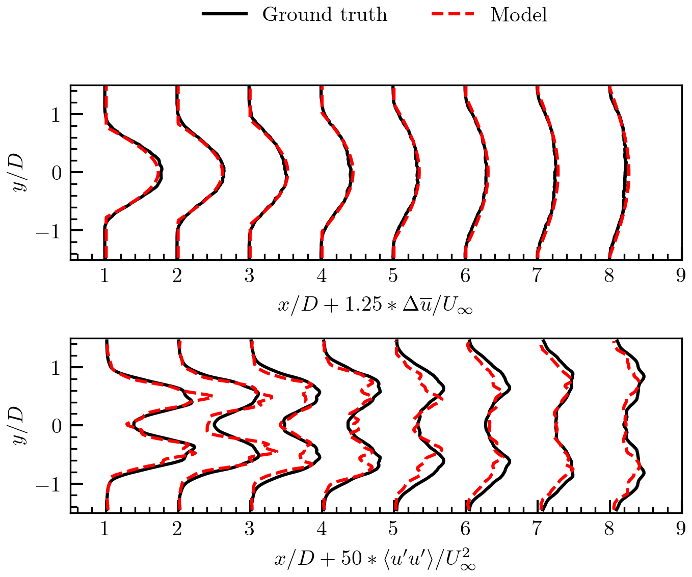
Figure B2 Time-averaged streamwise velocity deficit ($\mathrm{\Delta }\stackrel{\mathrm{‾}}{u}$) and variance of streamwise velocity fluctuation ($\langle u^{\prime }{u}^{\prime }\rangle$) profiles at various wind turbine downwind positions for downstream turbine(T₂). Solid black lines: reference LES results; dashed lines: model predictions for $\mathrm{\Delta }\stackrel{\mathrm{‾}}{u}$ and $\langle u^{\prime }{u}^{\prime }\rangle$. The normalized velocity deficit and variance are multiplied by constants C₁=1.25 and C₂=50, respectively, for better visual comparison of the relative spatial distributions in a single plot.

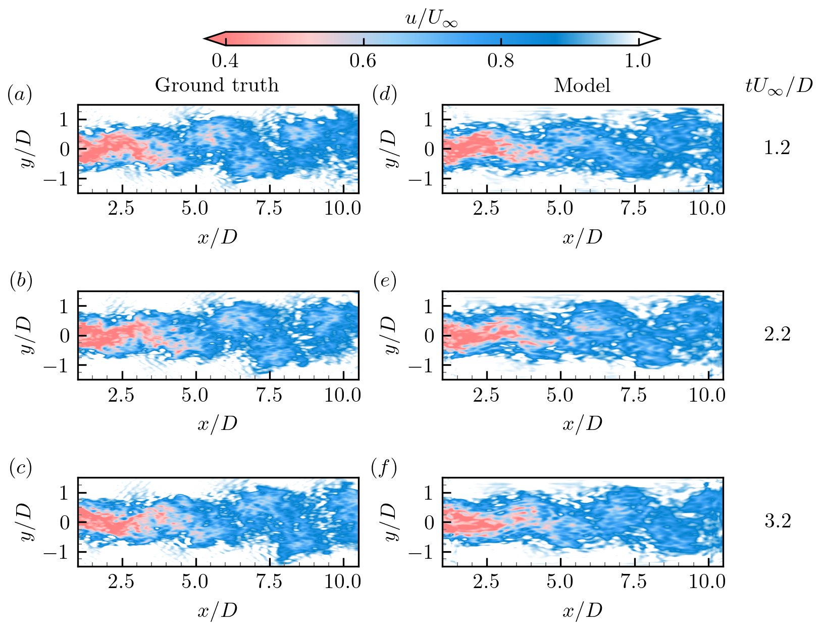
Figure B3 Instantaneous flow fields obtained from LES (a–c) and the proposed model (d–f) at the same instants. The contour is coloured by instantaneous streamwise velocity. The three rows from top to bottom correspond to three different instants, respectively.

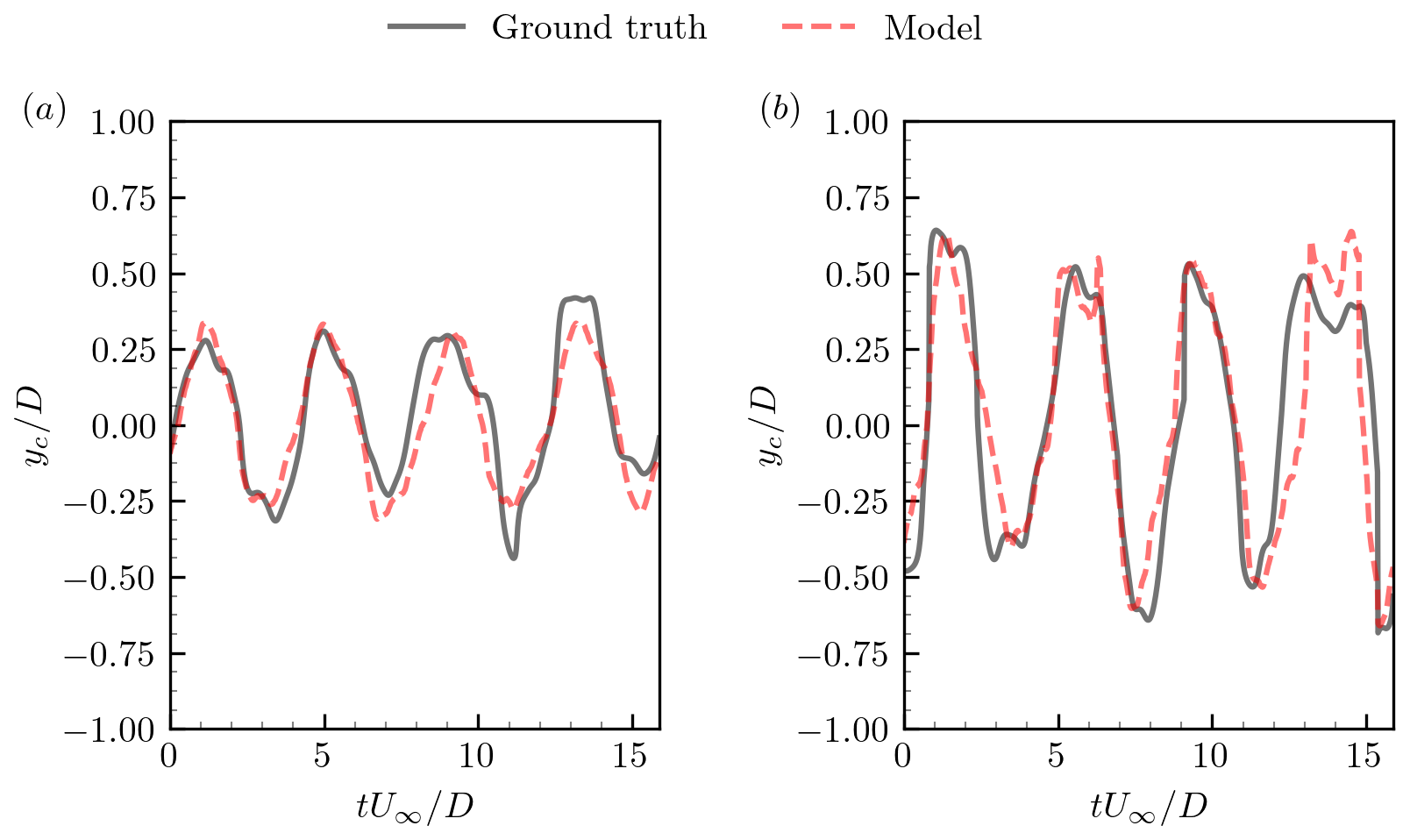
Figure B4 Comparison of temporal variations of spanwise wake centre positions (y_c, a–b)at the 5D and 10D downstream location. The solid lines and the dashed lines represent the results of LES and the proposed model, respectively.