Wind tunnel load measurements of a leading-edge inflatable kite rigid-scale model

Leading-edge inflatable (LEI) kites are morphing aerodynamic surfaces that are actuated by the bridle line system. Their design as tensile membrane structures has several implications for aerodynamic performance. Because of the pronounced C shape of the wings, a considerable part of the aerodynamic forces is redirected sideways and used for steering. The inflated tubular frame introduces flow recirculation zones on the pressure side of the wing. In this paper, we present wind tunnel measurements of a 1:6.5 rigid-scale model of the 25 m² TU Delft V3 LEI kite developed specifically for airborne wind energy (AWE) harvesting. Aerodynamic forces and moments were recorded in an open-jet wind tunnel over wide ranges of flow conditions, including angles of attack from −11.6 to 24.5°, sideslip angles from −20 to 20°, and freestream velocities from 5 to 25 m s⁻¹. The wind tunnel measurements were performed with and without zigzag tape along the model's leading edge to investigate the possible boundary layer tripping effect of the stitching seam connecting the canopy to the inflated tube. At a Reynolds number of 5×10⁵, the addition of zigzag tape was found to reduce lift and increase drag, indicating a negative impact on aerodynamic performance. The rigid-scale model was manufactured to match the undeformed geometry employed in Reynolds-averaged Navier–Stokes (RANS) simulations from the literature, rather than the unknown in-flight deformed geometry. A representative subset of the measurements was used to benchmark both these RANS and new vortex-step method simulations. Both computational methods successfully reproduced the measured trends under nominal operating conditions. While the post-stall discrepancy persists, excellent agreement was observed for lift, drag, and side force coefficients, with lift deviations remaining within the 10 % range.

1 Introduction

Airborne wind energy (AWE) systems use tethered flying devices to capture wind energy. The innovative technology promises to save up to 90 % of the material mass of conventional wind turbines (Van Hagen et al., 2023; Coutinho, 2024), resulting in a lower environmental footprint and potentially lower costs while providing access to previously untapped wind resources at higher altitudes (Bechtle et al., 2019; Kleidon, 2021). A prominent concept, which is also highly mobile, uses the pulling force of a soft kite manoeuvered in cross-wind patterns to drive a ground-based drum-generator module (Vermillion et al., 2021; Fagiano et al., 2022). Figure 1 illustrates the components of such an AWE system equipped with a leading-edge inflatable (LEI) kite with a suspended kite control unit (KCU). The kite operates in pumping cycles, alternating between traction and retraction phases, to generate a net positive power output. During the reel-out phase, the kite is guided in cross-wind flight patterns with its wing pitched to a high angle of attack. Once the tether reaches its maximum length, the cross-wind patterns are terminated, the wing is pitched to a low angle of attack, and the tether is retracted, using some of the previously generated and buffered energy. The cyclic operation results in a net energy gain because the aerodynamic force during the reel-out phase is substantially larger than the force in the reel-in phase, which is also shorter than the reel-out phase.

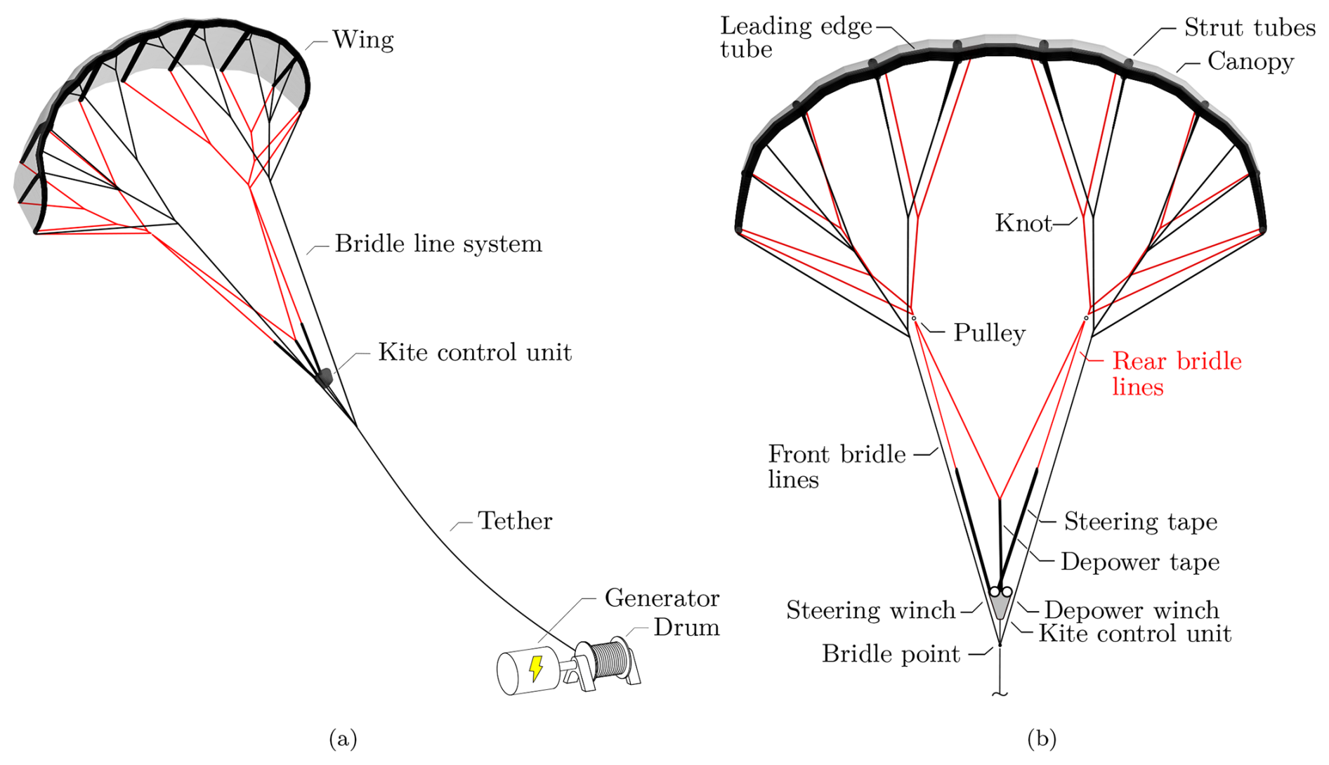
Figure 1 Ground-generating AWE system based on the TU Delft V3 kite, initially designed for a 20 kW technology demonstrator that was first used in 2012. (a) System overview, with tether and ground station depicted only schematically. (b) Components of the kite, consisting of the wing, bridle line system, and kite control. Adapted from Poland and Schmehl (2023).

Figure 1 further details the components and actuation layout of the kite. The KCU pitches and morphs the wing by adjusting the lengths of the rear bridle lines via the steering and depower tapes. Besides this actuation-induced deformation, the tensile membrane structure is also subject to strong aero-structural coupling (Oehler and Schmehl, 2019). The tubular frame of the wing consists of an inflatable leading-edge tube and several connected inflatable strut tubes. This frame provides structural stability for handling on the ground and for launching and landing, and, once the kite is in flight, it transmits the aerodynamic forces from the canopy to the bridle line system (Poland and Schmehl, 2023).

An optimal kite design can be regarded as an effective compromise between pulling force and controllability, acknowledging that both competing properties are tightly coupled. For instance, increasing the aspect ratio will generally increase the pulling force but decrease the agility of the kite. Similarly, making the wing flatter will increase its pulling force but decrease its steerability.

The aerodynamic properties of a kite have a major influence on the amount of wind energy that can be harvested. Accordingly, these properties play an important role in kite design, performance estimations, failure load prediction, and stability analysis for ensuring reliable and robust operation. A common approach for determining the aerodynamic properties of a given system is through in-flight experiments. One option that provides reasonable control over the inflow conditions is towing a small kite along a straight track to measure lift, drag, and dynamic response (Dadd et al., 2010; Python, 2017; Hummel et al., 2019; Rushdi et al., 2020; Elfert et al., 2024). A second option, applicable to larger industrial-scale kites, involves directly using sensor data from an operating AWE system to determine forces, position, and inflow conditions (Schmidt et al., 2017; Van der Vlugt et al., 2019; Oehler and Schmehl, 2019; Roullier, 2020; Schelbergen and Schmehl, 2024; Cayon et al., 2025). However, in-flight experiments are expensive, risky, and offer limited control over inflow conditions.

Numerical simulations offer a safer and more scalable alternative, which, due to actuation-induced morphing and strong aero-structural coupling, generally requires iterative resolution of both aerodynamic and structural mechanics (Breukels, 2011; Leloup et al., 2013; Bosch et al., 2014; Duport, 2018; Van Til et al., 2018). As system size increases, full-scale experimental characterization demands substantially more complex instrumentation, safety margins, and operational resources. In contrast, a validated computational model permits aerodynamic analysis of successively larger AWE systems at only modestly increasing computational cost, thereby enabling design-space exploration that would be impractical to achieve experimentally.

However, simulations necessitate validation, which is best achieved through wind tunnel testing that allows precise control of inflow conditions. Moreover, simulations are constrained by computational limitations – such as the need to ensure numerical stability and finite computational resources – which often necessitate simplifications such as Reynolds-averaged Navier–Stokes (RANS) modelling. Wind tunnel tests, therefore, enable not only validation, but also controlled, repeatable parametric studies that are difficult or impractical to perform numerically. Although wind tunnel experiments for LEI kites have not been reported in the public literature, related soft-wing structures have been described, including sail airfoil sections (Den Boer, 1980), paragliders (Nicolaides, 1971; Matos et al., 1998; Babinsky, 1999), ram-air wings (Wachter, 2008; Rementeria Zalduegui and Garry, 2019), and inflatable wings (Cocke, 1958; Smith et al., 2007; Okda et al., 2020; Desai et al., 2024).

One significant challenge for wind tunnel studies of industrial kites is that these membrane structures, which in 2025 typically range from 50 to 400 m², cannot be accommodated within standard wind tunnels and therefore necessitate downscaling. Aeroelastic effects complicate scaling because maintaining the correct proportion of structural to aerodynamic loads is non-trivial, as highlighted by Oehler et al. (2018). Additionally, developing such models encounters manufacturing and structural material limitations; for instance, adjusting beam bending stiffness would necessitate impractically high inflation pressures. Lastly, comparing experimental data to aero-structural coupled simulations lacks specificity, making it unclear whether discrepancies arise from errors in modelling aerodynamics, structural dynamics, coupling mechanisms, or other factors.

Wind tunnel experiments using rigid-kite models eliminate the aeroelastic scaling issues and provide aerodynamic data with a high degree of certainty on the inflow. Belloc (2015) presented wind tunnel measurements of a 1:8 scale paraglider model, in which the anhedral angle – defined as the downward inclination of the wing relative to the horizontal plane when viewed from the front – follows an elliptical shape, and the model incorporates a spar made of a wood–carbon composite sandwich. During the tests, inflow velocities reached 40 m s⁻¹, corresponding to Reynolds numbers of 9.2×10⁵. The experiments covered angles of attack ranging from −5 to 22° and sideslip angles from −15 to 15°. The results showed that the arched paraglider wing exhibits distinct aerodynamic behaviour compared to a flat wing, especially in lateral dynamics. Wing curvature couples sideslip angle to the local angle of attack, thereby modulating the spanwise lift distribution. This redistribution of lift generates a lateral force and a nose-down pitching moment, produces a stabilising yawing moment, and induces a rolling moment that raises the wingtip opposite to the sideslip direction, a mechanism commonly referred to as pendulum stability.

Omitting deformation isolates the aerodynamic problem and provides the necessary specificity to validate simulations. The literature reports LEI kite aerodynamic simulations ranging from low-fidelity potential flow methods to high-fidelity computational fluid dynamic (CFD) methods. The potential flow methods are often a form of Prandtl (1918) lifting-line theory, and to increase accuracy, most models include the addition of nonlinear section lift–curve slopes, i.e. airfoil polars (Leloup et al., 2013; De Solminihac et al., 2018; Cayon et al., 2023). The airfoil polar aerodynamic simulations should incorporate viscosity and vorticity to accurately represent the generally present separation zone aft of the inflatable tube, e.g. using RANS CFD (Breukels, 2011; Folkersma et al., 2019; Watchorn, 2023). RANS CFD simulations have also been conducted in three dimensions for the TU Delft V2 kite (Deaves, 2015) and for the V3 kite with and without struts (Viré et al., 2020, 2022).

The present paper is based on the graduation project of Van Spronsen (2024), presenting a novel wind tunnel experiment of an LEI kite to acquire validation data for numerical tools. The aerodynamic characteristics of a rigid-scale model of the V3 kite were obtained over an extensive range of inflow conditions, with a high degree of certainty regarding the match between simulated and measured geometry and inflow conditions. Thorough analysis of potential sources of uncertainty reinforced the reliability of the measured aerodynamic loads. In addition, the effects of forced boundary layer transition, Reynolds number variation, and sideslip were examined in detail. Measured aerodynamic forces and moments were compared with numerical simulations to assess the consistency between experimental and computational results.

The remainder of this paper is organized as follows. Section 2 describes the experimental methodology. Section 3 presents the results of our wind tunnel tests, focusing on analysing the uncertainties and the effect of Reynolds number. A discussion on the agreement with numerical predictions follows in Sect. 4, and the conclusions are presented in Sect. 5 along with recommendations for future work.

2 Experimental methodology

This section first discusses the specifics of the wind tunnel and the scale model. This is followed by a description of the experimental setup, measurement matrix, zigzag tape measurements, and data processing method, including the required wind tunnel corrections.

2.1 Open Jet Facility

The wind tunnel experiments were conducted in the Open Jet Facility (OJF) at the Faculty of Aerospace Engineering of Delft University of Technology from 1 to 10 April 2024. The facility is a closed-loop wind tunnel, featuring an octagonal jet exhaust nozzle with maximum dimensions of 2.85 m×2.85 m and a contraction ratio of 3:1, as illustrated in Fig. 2. The jet discharges into a test section room with dimensions 13 m in width and 8 m in height. The wind tunnel is equipped with a 500 kW electric motor driving a large fan, which generates a controlled streamwise velocity of up to 35 m s⁻¹ in the test section. Corner vanes and wire meshes guide the flow to ensure uniform flow conditions, resulting in a turbulence intensity of 0.5 % in the test section (Lignarolo et al., 2014).

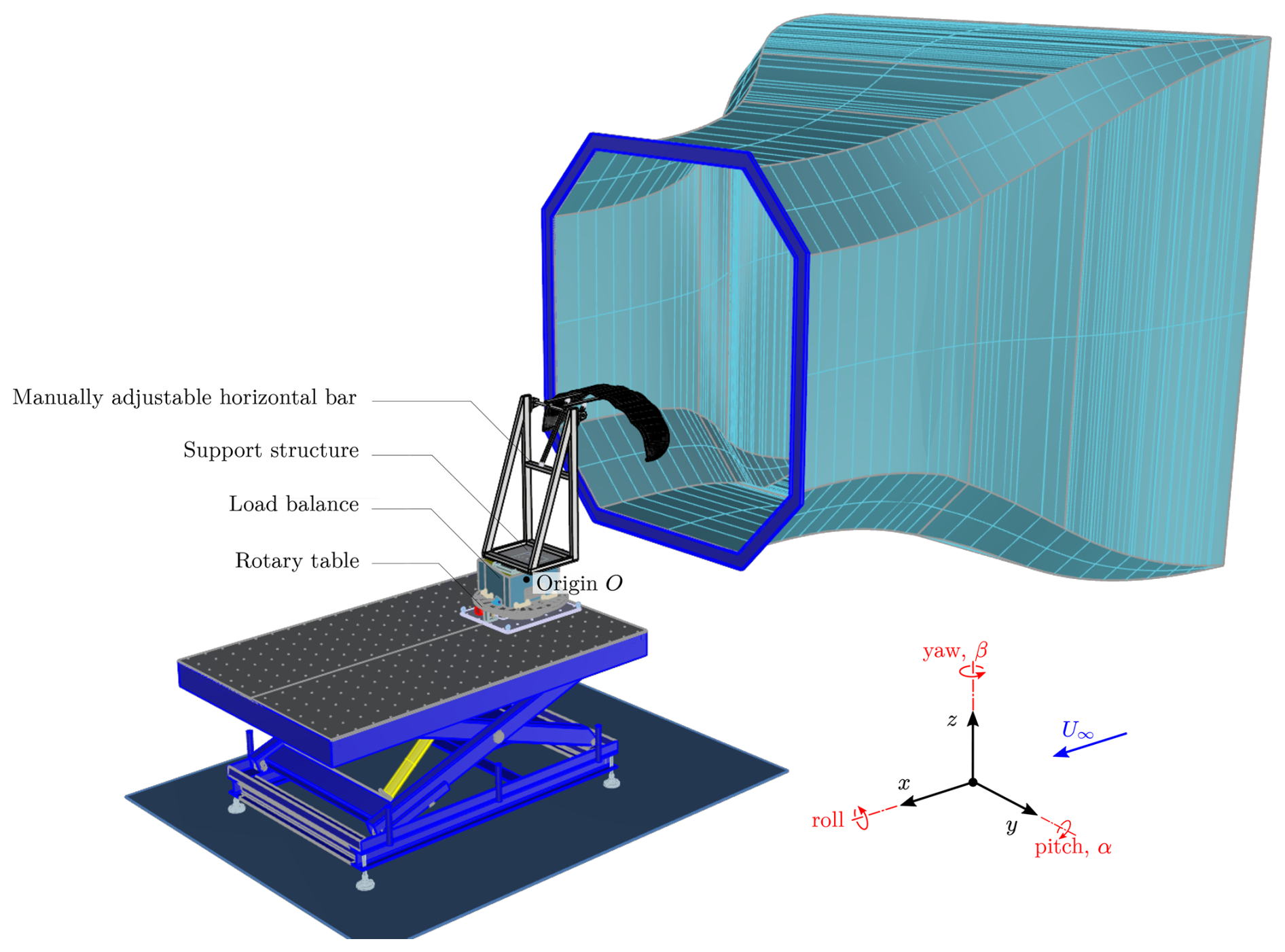
Figure 2 CAD drawing of the experimental setup, showing the origin O in the load balance representing the point at which the load measurements are made. With a sideslip angle β=0°, the x axis runs along the longitudinal direction of the wind tunnel, pointing downstream parallel to the wind. The y axis is oriented laterally, pointing to the right when facing upstream, or, from the kite's perspective, right when looking from the trailing edge towards the leading edge. The z axis is vertical, pointing upwards. The rotary table, load balance, support structure, and kite are all placed on the blue table, which was adjusted in lateral position and height to centre the model in the nozzle exit.

2.2 Rigid-scale model

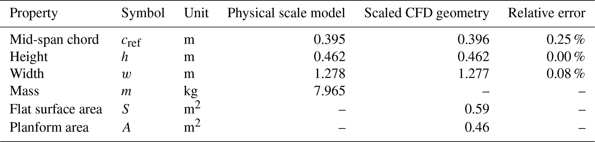
As the original TU Delft LEI V3 kite is 8.3 m wide and the width of the OJF exhaust nozzle is only 2.85 m, a scale model had to be used. With the main purpose of the measurement campaign being the acquisition of validation data for numerical tools, the scale model was manufactured to match the wing geometry used in earlier CFD simulations (Viré et al., 2022). This geometry was adapted from the original design CAD model to facilitate mesh smoothness in the simulations. Notably, the bridle line system was omitted, the trailing edge connecting the upper and lower canopy surfaces was rounded, and an edge fillet was applied at all canopy–tube junctions. The only difference between the CFD and manufactured geometries is the use of a canopy with increased thickness for structural integrity – 3 to 4 mm instead of 1 mm. The model geometry was verified using a laser tracker with a spatial resolution of 0.5 µm (FARO, 2024). Figure 3 compares the manufactured physical model with the rendered geometry and the overlaid laser-tracked outline of the physical model. The agreement between the manufactured and rendered geometry was within 1 mm in chord, height, and width, corresponding to errors of less than 0.25 % in all cases, as detailed in Table 1.

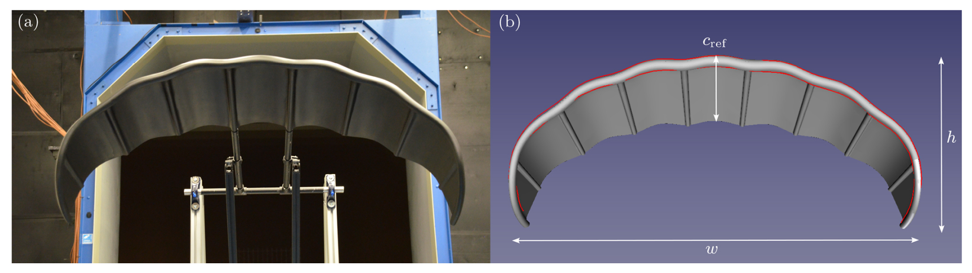
Figure 3 Rigid-scale model of the TU Delft LEI V3 kite. (a) Photograph of the model, rotated by 180°, with its back facing the blue octagonal OJF exhaust nozzle. (b) Rendering of the model from a similar perspective, with the laser-tracked outline overlaid in red and the reference chord c_ref, height h, and width w indicated in white.

Table 1 Properties of the rigid-scale model, including values for the physical scale model and the scaled design geometry. The physical model properties were measured using a laser tracker, while the scaled design geometry values correspond to the scaled design geometry of the kite. The relative error between the physical model and the scaled design geometry is also provided.

Considering manufacturing costs, handling limitations, Reynolds number scaling, and wind tunnel blockage, further detailed in Appendix B, we decided on a 1:6.5 scaling of the wind tunnel model, leading to the dimensions listed in Table 1. The anhedral swept wing with a bow-shaped leading edge and double-curved canopy was manufactured by Curveworks B.V. using carbon-fibre-reinforced plastic laid up in a 3D-milled mould from structural foam. The canopy is 3 mm thick, except for the two central panels, which are 4 mm as they need to sustain a higher load. The outer layers provided the most structural support and were made of carbon fibre. The 1 or 2 mm inner layers were made of a glass-fibre-reinforced polymer. Structural foam was used inside the chordwise struts, except for the two inner struts, which incorporate two parallel steel rods. These rods slide into the two aluminium sleeve tubes of the support frame, as illustrated in Fig. 3a.

2.3 Measurement equipment

The support frame is a truss structure assembled from custom-cut aluminium profiles. The angle of attack α quantifies the inclination of the mid-span chord line with respect to the inflow and can be adjusted as illustrated in Fig. 4. The angle was measured with an accuracy of 0.1° by placing two digital inclinometers on the aluminium sleeve tubes. The measured value is converted to the angle of attack α by subtracting the offset angle 6.3° between the chord line and the parallel steel rods of the model. The support structure was placed aft of the kite to minimize flow interference and mounted onto a six-component load balance, as illustrated in Fig. 2. The balance operates at 2000 Hz and is equipped with six load cells able to measure the longitudinal, inflow-aligned F_x, transverse F_y, and vertical F_z forces and the roll M_x, pitch M_y, and yaw M_z moments. The entire assembly was mounted on a rotary table, allowing a remote adjustment of the sideslip angle β with an angular resolution of 0.01°. The sideslip angle was defined in a body-fixed reference frame. A counter-clockwise rotation of the turn-table, which appeared as a positive rotation in Fig. 2, therefore corresponded to a negative inflow angle  β  in the body-fixed reference frame.

Figure 4 Manual setting of the scale model's angle of attack with respect to the inflow by adjusting the vertical position of the strut attachment to the support structure. The centre of gravity of the scale model is indicated by point CG.

2.4 Measurement matrix

The experiments were conducted for most combinations of α, β, and U_∞ listed in Table 2, although time constraints prevented testing all β values at every α. The test matrix was designed to cover the full range of inflow conditions encountered in flight. Based on in-flight measurements, the angle of attack α typically varied between 1° during reel-in and 8° during reel-out (Cayon et al., 2025), while observed sideslip angles β generally remained within −10 to 10° (Oehler et al., 2018). Table 2, therefore, includes these operational ranges of α and β to ensure that the inflow conditions experienced by the V3 kite are represented, and additional values of both angles are incorporated to provide further data points for model validation.

Table 2 Parametric combinations investigated with wind tunnel measurements.

The Reynolds number,

$$\begin{array}{}\text{(1)}& {\displaystyle }{\displaystyle }\mathit{Re}={\displaystyle \frac{U_{\mathrm{\infty }}{c}_{\text{ref}}}{\mathit{\nu }}},\end{array}$$

was used to characterize the flow regime, recalculating the kinematic viscosity ν for each value of U_∞ using Sutherland's law (Poling et al., 2001). Multiple inflow speeds were included to assess the influence of varying Re, and those listed in Table 2 were selected to approach in-flight values. The experimental setup did not permit matching the in-flight Re, which for the V3 kite was around $\mathit{\text{Re}}=\mathrm{3}\times {\mathrm{10}}^{\mathrm{6}}$ (Cayon et al., 2025).

Measurements without the kite were performed across the full parameter range to quantify the aerodynamic loads on the support structure alone. As the load measurement setup did not permit quantification of the interference between the structure and the kite, these effects were assumed to be negligible. To ensure consistency, measurements taken with α=5.7° at U_∞=20 m s⁻¹ and $\mathit{\beta }=-\mathrm{20}$, 0, and 20° were repeated three times. Furthermore, the sensor drift of the load balance during the campaign was analysed through six measurements done over a 30 s time interval each morning and evening with U_∞=0 m s⁻¹ for 3 consecutive days. A zero-wind measurement was performed before each measurement set, and by using this as a baseline, any sensor drift present in the system was inherently accounted for in the subsequent data.

A measuring period of 10 s was selected for all tests. Given that approximately 125–625 fluid parcels pass within this time, combined with the agreement between repeated measurements and the outcome of a dedicated convergence analysis, the measuring period was deemed statistically sufficient; further details are provided in Appendix A.

2.5 Laminar–turbulent flow transition

Using two-dimensional (2D) CFD simulations, Folkersma et al. (2019) showed that incorporating a boundary layer transition model significantly affects the aerodynamic predictions for $\mathit{\text{Re}}<\mathrm{2}\times {\mathrm{10}}^{\mathrm{7}}$. This motivated the use of natural transition modelling in subsequent three-dimensional (3D) CFD simulations of the V3 kite (Viré et al., 2020, 2022). In practice, transition may be influenced by the zigzag-patterned stitching seam connecting the canopy to the tube along the span, as shown in Fig. 5a. Whether this seam height would be sufficient to induce transition remained uncertain, however. As the scale model did not incorporate this stitching seam, additional measurements using zigzag tape were conducted to address this issue. The setup is shown in Fig. 5b.

Figure 5 (a) Kitepower V3.25B kite with seams along the leading edge. (b) Scale model with zigzag tape applied to the leading edge. Although they have slightly different designs, the V3.25B and TU Delft V3 kites are practically identical with respect to the flow over the wing's suction side.

The critical roughness Reynolds number Re_k,crit is commonly used to quantify the height threshold at which a surface roughness element induces boundary layer transition. The numerical estimation of this number is non-trivial, as it depends on local pressure gradients, freestream disturbances, geometry, and roughness characteristics (Ye, 2017). In practice, trip heights are often estimated through empirical correlations (Langel et al., 2014; Gahraz et al., 2018). Braslow and Knox (1958) reported typical values of Re_k,crit ranging between 300–600. For zigzag or wavy-patterned 2D roughness, Balakumar (2021) adopted a value of 300, while others found 200 to be sufficient (van Rooij and Timmer, 2003; Elsinga and Westerweel, 2012). Given a value of Re_k,crit, the corresponding roughness height k can be computed using the relation (Braslow and Knox, 1958)

$$\begin{array}{}\text{(2)}& {\displaystyle }{\displaystyle }k={\displaystyle \frac{{\mathit{\text{Re}}}_{k,\text{crit}}\mathit{\nu }}{U_k}},\end{array}$$

where U_k denotes the local velocity at the roughness height, which lies within the boundary layer and is therefore different from the external velocity U_∞, i.e. generally somewhat smaller; nonetheless, it is often approximated by U_∞ for practical purposes (Driest and McCauley, 1960; Tani, 1969). For a more precise assessment, the local velocity profile within the boundary layer could be employed to determine U_k directly; however, this typically necessitates either supplementary measurements or detailed boundary layer computations, which were not available in the present study. The resulting functional dependency of k is shown in Fig. 6 for two different values of Re_k,crit. The diagram also includes the selected tape height of 0.2 mm to trigger transition from approximately $\mathit{\text{Re}}\ge \mathrm{3.9}\times {\mathrm{10}}^{\mathrm{5}}$ according to the estimate ${\mathit{\text{Re}}}_{k,\text{crit}}=\mathrm{200}$. The tape, produced by Glasfaser Flugzeug-Service GmbH with a 60° tooth angle, was applied at 5 % chord, following the approach in Soltani et al. (2011), Gahraz et al. (2018), Dollinger et al. (2019), and De Tavernier (2021).

Figure 6 Required minimal trip height vs. Re for different values of Re_k,crit.

2.6 Data post-processing

The measured load data were converted to the non-dimensional aerodynamic coefficients as follows:

1. subtract zero-wind measurements

2. non-dimensionalize the load data

3. translate the coordinate system from the load balance origin O to the centre of gravity of the scale model

4. correct for sideslip

5. subtract non-dimensionalized support-structure loads

6. apply wind tunnel corrections.

• (1)

  First, the zero-wind measurements taken before every α change were subtracted to eliminate background noise from the signals, including the structure's weight and sensor drift.

• (2)

  In the next step, the measurements were non-dimensionalized using the air density ρ, determined at each measurement point, varying from 1.14 to 1.19 kg m⁻³; the inflow speed U_∞; the projected area A; and the reference chord c_ref of the scale model, as listed in Table 1. The forces F_i and moments M_i,b were non-dimensionalized using

  $$\begin{array}{}\text{(3)}& {\displaystyle }{C}_i={\displaystyle \frac{\mathrm{2}{F}_i}{\mathit{\rho }{U}_{\mathrm{\infty }}^{\mathrm{2}}A}},i=\mathrm{1},\mathrm{2},\mathrm{3},\text{(4)}& {\displaystyle }{C}_{\text{M,i,b}}={\displaystyle \frac{\mathrm{2}{M}_{i,b}}{\mathit{\rho }{U}_{\mathrm{\infty }}^{\mathrm{2}}A{c}_{\text{ref}}}},i=\mathrm{1},\mathrm{2},\mathrm{3}.\end{array}$$
• (3)

  To represent the moment coefficients in the wing reference frame, they had to be translated from the load balance measurement centre to the centre of gravity CG of the scale model. When the mid-span chord line is aligned with the x axis, the CG is located at −0.172 m in the x direction and −0.229 m in the z direction with respect to the mid-span trailing-edge point; see Fig. 4. The distance from the origin O to the CG varied with angle of attack but remained constant with sideslip, as the load balance was mounted atop the rotary table and therefore rotated with it. The rolling moment coefficient $C_{\mathrm{M},x,b}$ is translated using

  $$\begin{array}{}\text{(5)}& {\displaystyle }{\displaystyle }{C}_{\mathrm{M},x}=C_{\mathrm{M},\mathrm{x},\mathrm{b}}-C_{F,y}{z}_{\text{cg}}.\end{array}$$

  The pitching- and yawing-moment coefficients, C_M,y and C_M,z, respectively, were determined as

  $$\begin{array}{}\text{(6)}& {\displaystyle }& {\displaystyle }{C}_{\mathrm{M},y}=-C_{\mathrm{M},y,b}+C_{F,z}{x}_{\text{cg}}-C_{F,x}{z}_{\text{cg}},\text{(7)}& {\displaystyle }& {\displaystyle }{C}_{\mathrm{M},z}=-C_{F,z,b}-C_{F,y}{x}_{\text{cg}}.\end{array}$$

  In these expressions, x_cg, y_cg, and z_cg are the coordinates of the scale model's centre of gravity, with respect to O.

• (4)

  Because the load balance was mounted on top of the rotary table and y is defined perpendicular to the incoming flow, the force and measured moment coefficients had to be corrected for the sideslip. The force and moment coefficient vectors were transformed, at each sideslip angle β_i, through matrix multiplication by the rotation matrix R:

  $$\begin{array}{}\text{(8)}& {\displaystyle }{\displaystyle }\mathbf{R}=\left[\begin{array}{ccc}\cos \mathit{\beta }& \sin \mathit{\beta }& \mathrm{0}\\ -\sin \mathit{\beta }& \cos \mathit{\beta }& \mathrm{0}\\ \mathrm{0}& \mathrm{0}& \mathrm{1}\end{array}\right].\end{array}$$
• (5)

  To isolate the aerodynamic forces of the kite, measurements were made with only the support structure. These measurements were performed at the minimum, mean, and maximum α values. Missing data points were determined by interpolation, which was carried out by fitting two linear segments from the minimum to the mean and from the mean to the maximum, respectively. A two-segment linear fit was selected as it captured the measured trends, whereas a single linear fit failed to do so, and parabolic fits overfitted near the bounds.

  The aerodynamic loads on the support structure only were measured and processed through steps (1)–(4) such that the resulting aerodynamic coefficients could then be subtracted from the coefficients of the kite including the support structure. It was critical to non-dimensionalize before subtracting these measurements, as atmospheric conditions could not be assumed constant throughout the experiment. Specifically, during the experiment, the temperature varied between 20–32°C.

• (6)

  The last step entailed applying the wind tunnel corrections that arise from blockage, streamline curvature, and downwash or upwash in both y and z directions. For a detailed analysis of these effects, the reader is referred to Appendix B. The conclusions were that with a blockage factor of 3 %, the corrections due to blockage are negligible, which aligns with the recommendations of Wickern (2014) to keep the blockage factor below 5 % and of Barlow et al. (1999) to stay below 7.5 %. Following Barlow et al. (1999), the corrections due to streamline curvature and downwash were calculated and found to be non-negligible, shown in Table B1, and hence applied.

3 Results

This section first addresses the measurement uncertainties, followed by the effect of forced boundary layer transition. Subsequently, the aerodynamic force and moment coefficients are presented as functions of the angle of attack and the sideslip angle over the measured range of Re.

3.1 Uncertainty analysis

This section quantifies the main sources of measurement uncertainty to ensure data reliability and repeatability, including sensor drift, support-to-kite load proportion, vibration analysis, coefficient of variation, and measurement repeatability. Although a load balance sensor drift was detected, it was concluded not to affect the results, as detailed in Appendix C. Analysing the proportions of support-structure loads to kite loads as signal-to-noise ratio, one finds high certainty for lift and lower certainty for C_M,y and C_M,z, as detailed in Appendix D.

For some measurements at U_∞=25 m s⁻¹ and high values of α and β, the wind tunnel model started to vibrate considerably. To avoid physical damage, these specific measurements were not completed, which is why some data points are missing at $\mathit{\text{Re}}=\mathrm{6.1}\times {\mathrm{10}}^{\mathrm{5}}$. A vibration analysis revealed structural resonance at 4–5 Hz, close to the resonance frequency of the supporting blue table shown in Fig. 2, as reported in LeBlanc and Ferreira (2018). This frequency band was not filtered to avoid introducing processing artefacts. See Appendix E for further details, i.e. time series and power spectral density analyses.

The coefficient of variation, denoted as CV, offers a dimensionless metric for comparing variability across different datasets by normalizing the standard deviation relative to the mean (Pearson, 1896). For each aerodynamic force or moment coefficient,

$${\displaystyle }{\text{CV}}_i={\displaystyle \frac{\stackrel{\mathrm{‾}}{{\mathit{\sigma }}_i}}{{\mathit{\mu }}_i}},i\in \mathit{\{}L,D,\mathrm{S},M_x,M_y,M_z\mathit{\}},$$

where $\stackrel{\mathrm{‾}}{{\mathit{\sigma }}_i}$ is the average standard deviation of coefficient i, and μ_i is its mean value, both computed over the ensemble of measurements. Table 3 lists CV_i for each Re, except for $\mathit{\text{Re}}=\mathrm{6.1}\times {\mathrm{10}}^{\mathrm{5}}$, which is excluded due to incomplete data. The means μ_i were computed over the full range of α and β for CV_L, CV_D, and CV_M,y. For CV_S, CV_M,x, and CV_M,z, only positive values of β were considered to avoid including near-zero loads at β=0°, which could lead to inflated values of CV_i and skew the statistical averages.

Table 3 Coefficient of variation CV_i of the data for varying Re.

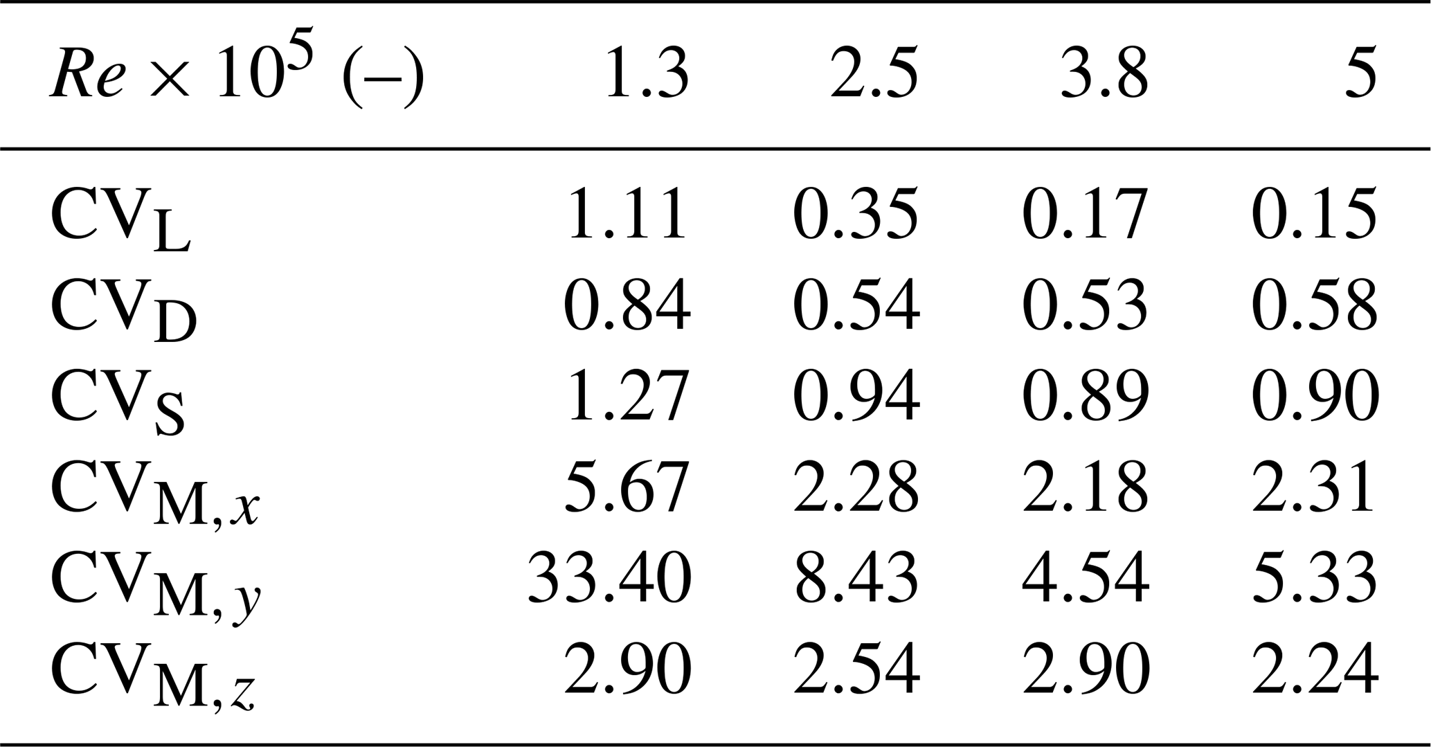
The decline in CV_i values from Re=1.3 to 2.5×10⁵ reflects a reduction in relative measurement uncertainty, as the standard deviation becomes smaller relative to the mean. In this work, force measurements exhibited lower relative uncertainty compared to moment measurements, which can be attributed to their inherently higher signal-to-noise ratios. The cases at Re=3.8 and 5×10⁵ exhibit the smallest values of CV_i, indicating the highest relative measurement precision. However, it should be noted that a low CV reflects only the precision – that is, the spread or random uncertainty of the measurements – and does not account for possible systematic errors or constant offsets that may affect accuracy.

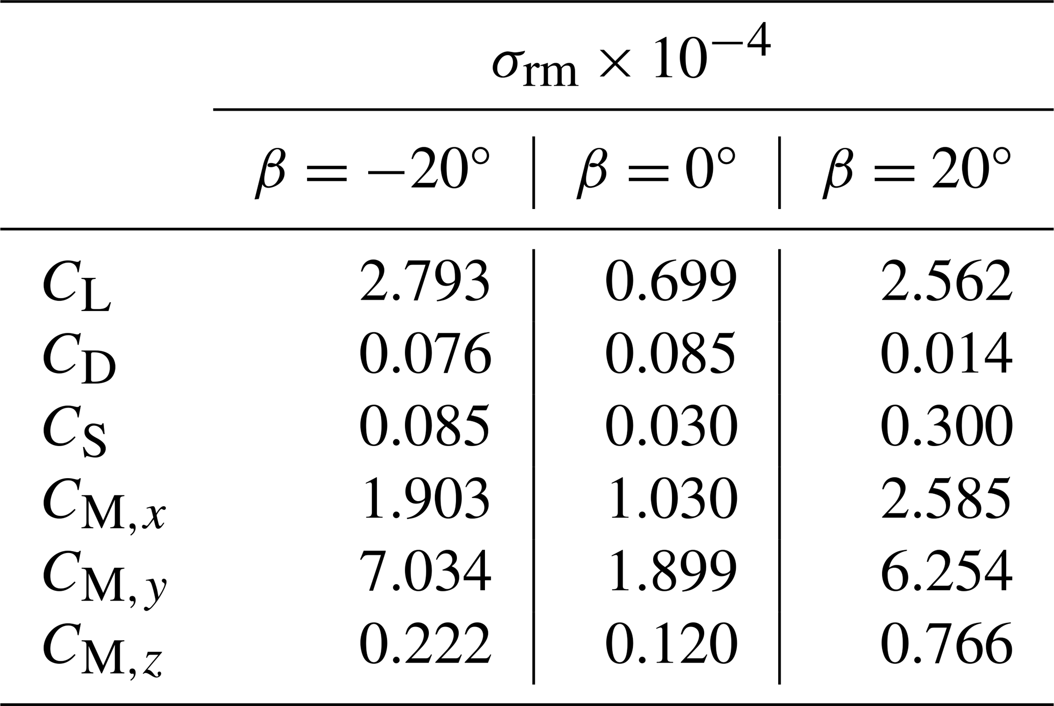
At $\mathit{\text{Re}}=\mathrm{5}\times {\mathrm{10}}^{\mathrm{5}}$; α=5.7°; and $\mathit{\beta }=-\mathrm{20}$, 0, and 20°, measurements were made three times to check the repeatability. For each of these measurements, the standard deviation within these repeated measurements σ_rm is shown in Table 4. The authors conclude that the measurement repeatability is overall high, as evidenced by the orders of magnitude difference between the averaged standard deviation, $\mathrm{1}\times {\mathrm{10}}^{-\mathrm{1}}$, and the repeatability standard deviation, $\mathrm{1}\times {\mathrm{10}}^{-\mathrm{4}}$. The smallest uncertainties are for β=0°.

Table 4 Standard deviations of the repeatability measurements σ_rm for three β values taken with α=5.7°.

3.2 Effect of forced boundary layer transition

The measured aerodynamic force coefficients with and without zigzag tape are shown in Fig. 7 for β=0° and α=9.4°, selected for its proximity to the nominal reel-out angle of α=8° (Cayon et al., 2025). The $\mathit{\text{Re}}=\mathrm{6.1}\times {\mathrm{10}}^{\mathrm{5}}$ case was excluded due to missing data. In addition to the mean values, a confidence interval (CI) is plotted, indicating with 99 % certainty that the mean lies within the given range. As detailed in Sect. 2.4, the load balance records data over a 10 s time interval, thereby capturing between 125–625 fluid parcels passing through. The resulting samples are regarded as temporally correlated; one supporting argument is that each fluid element traverses the measurement region over 16–80 ms, while data are sampled at much finer 0.5 ms intervals. To accurately estimate the sample measurement uncertainty of this correlated time series, the heteroskedasticity and autocorrelation-consistent (HAC) estimator by Newey and West (1987) is employed. The method requires an estimate of the time lag. A time lag of 11 samples was found from taking the integer value of $N_{\text{samples}}^{\frac{\mathrm{1}}{\mathrm{4}}}$ (Greene, 2019).

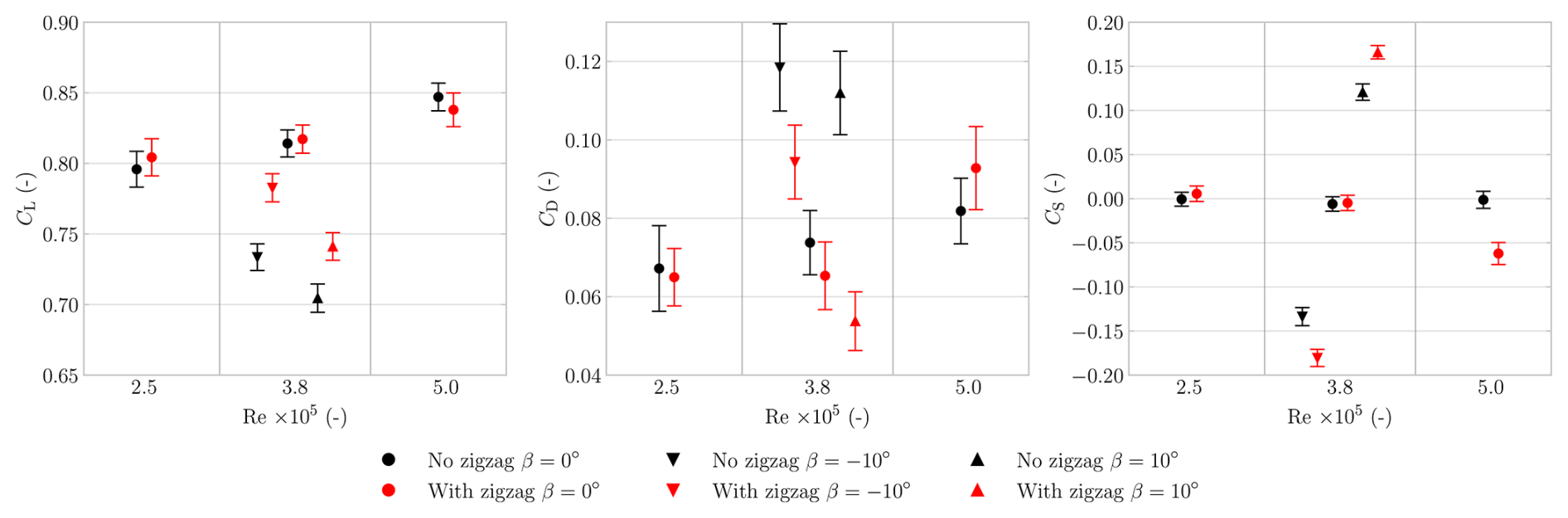
Figure 7 Aerodynamic force coefficients plotted with standard deviation, with and without zigzag tape, at Re=1.3, 2.5, 3.8, and 5×10⁵, at an averaged corrected α=9.4°.

For context, the theoretical analysis leading to Fig. 6 indicated that a zigzag tape height of 0.2 mm would be insufficient to force transition at $\mathit{\text{Re}}=\mathrm{2.5}\times {\mathrm{10}}^{\mathrm{5}}$, marginally sufficient at 3.8×10⁵, and sufficient at 5×10⁵. The three horizontally separated regions in Fig. 7 correspond to these different Re, with black and red symbols indicating measurements obtained without and with zigzag tape, respectively. At β=0°, adding zigzag tape resulted in higher lift and lower drag for Re=2.5 and 3.8×10⁵, whereas the opposite trend was observed at $\mathit{\text{Re}}=\mathrm{5}\times {\mathrm{10}}^{\mathrm{5}}$, including a 12 % increase in drag. This latter observation is consistent with the literature, where the introduction of zigzag tape led to decreased lift and increased drag (Gahraz et al., 2018; Zhang et al., 2017a, b; Dollinger et al., 2019).

Definitive conclusions cannot be drawn for the non-zero sideslip cases, where data are limited to $\mathit{\text{Re}}=\mathrm{3.8}\times {\mathrm{10}}^{\mathrm{5}}$ at α=9.4° for $\mathit{\beta }=\pm \mathrm{10}\mathrm{°}$. Nonetheless, based on the measured increase in lift and side force, along with an observed 50 % reduction in drag, the authors hypothesize that, in the sideslip configuration, the zigzag tape may locally promote a laminar-to-turbulent transition that delays flow separation.

Without zigzag tape and under sideslip, the measured C_S value remains near zero, independent of Re. In contrast, with zigzag tape, a negative C_S is observed at $\mathit{\text{Re}}=\mathrm{5}\times {\mathrm{10}}^{\mathrm{5}}$. This difference suggests that the zigzag tape introduces a setup asymmetry, possibly due to imperfect tape application.

3.3 Reynolds number effects

Figure 8 presents the measured force and moment coefficients as functions of α for various Re. In the measurements, the lift coefficient C_L increases with Re but so does the drag coefficient C_D, resulting in a $C_{\mathrm{L}}/C_{\mathrm{D}}$ ratio that does not show a consistent increasing trend with Re, except for the $\mathit{\text{Re}}=\mathrm{6.1}\times {\mathrm{10}}^{\mathrm{5}}$ case. This finding contrasts with the 3D numerical simulations of Viré et al. (2022), in which both an increase in lift and a decrease in drag were observed from $\mathit{\text{Re}}=\mathrm{1}\times {\mathrm{10}}^{\mathrm{5}}$ to 1×10⁶, leading to higher $C_{\mathrm{L}}/C_{\mathrm{D}}$ with increasing Re. The absence of a similar trend in the present measurements may be attributed to the smaller range of Re realized experimentally, differences in canopy thickness, and/or drag underprediction in the simulations, as discussed in Sect. 4.

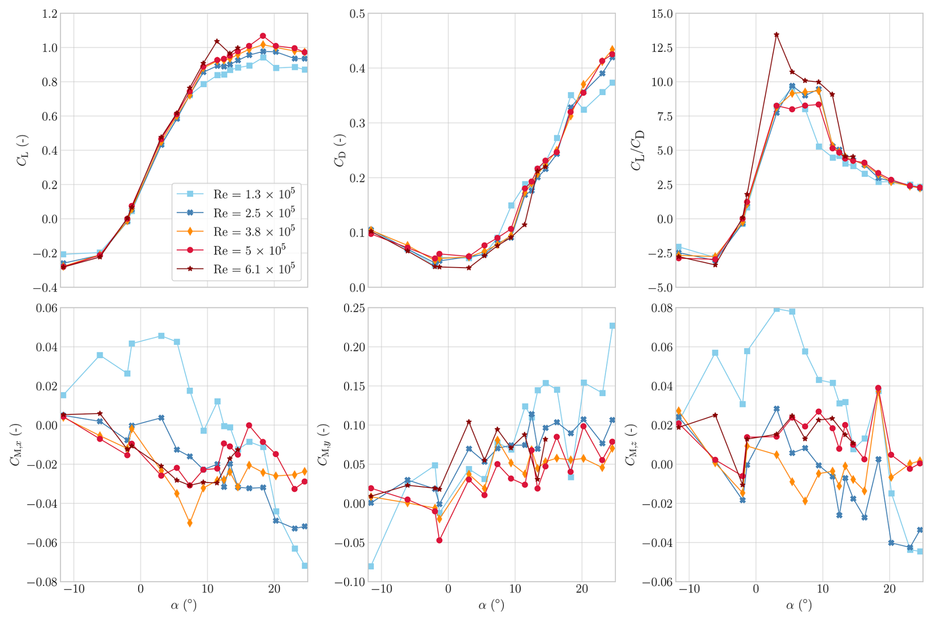
Figure 8 Aerodynamic force and moment coefficients plotted against α for Re varying from 1.3×10⁵ to 6.1×10⁵ at β=0°.

The $\mathit{\text{Re}}=\mathrm{1.3}\times {\mathrm{10}}^{\mathrm{5}}$ case exhibits the least smooth curves, attributable to a less favourable signal-to-noise ratio; i.e. the load magnitudes are relatively small compared to the support-structure loads. The C_L–α plot suggests that, compared to higher Re, stall development may occur at lower angles, as evidenced by the earlier decrease in slope of the C_L–α curve for $\mathit{\text{Re}}=\mathrm{1.3}\times {\mathrm{10}}^{\mathrm{5}}$, indicating reduced lift growth and hence the possible onset of local flow separation. This aligns with aerodynamic theory predicting earlier separation in laminar flows due to lower sensitivity to adverse pressure gradients (Anderson, 2016).

Although small in magnitude, the non-zero values of C_M,x and C_M,z may have indicated an asymmetry in the setup. For coefficients of smaller magnitude, the non-smoothness of the curves was amplified, which was consistent with the higher relative uncertainties found, as indicated by the coefficient of variation in Table 3. The pitching moment coefficient C_M,y exhibited an increasing trend with increasing α.

The influence of β, shown in Fig. 9, was examined at α=7.4°, as this condition most closely resembled the average angle of attack of 8° observed during the reel-out phase of a V3 kite flight (Cayon et al., 2025). A perfectly symmetric setup would yield coefficients C_L, C_D, and C_M,y symmetric about β=0° and coefficients C_S, C_M,x, and C_M,z that are antisymmetric. In practice, slight asymmetries in the experimental setup caused small deviations from this ideal symmetry, notably non-zero values of C_S, C_M,x, and C_M,z at β=0°, as well as minor asymmetries of C_L, C_D, and C_M,y about the vertical axis. The largest deviations from ideal symmetry were observed at the lowest $\mathit{\text{Re}}=\mathrm{1.3}\times {\mathrm{10}}^{\mathrm{5}}$, with overall increasing symmetry as Re increased.

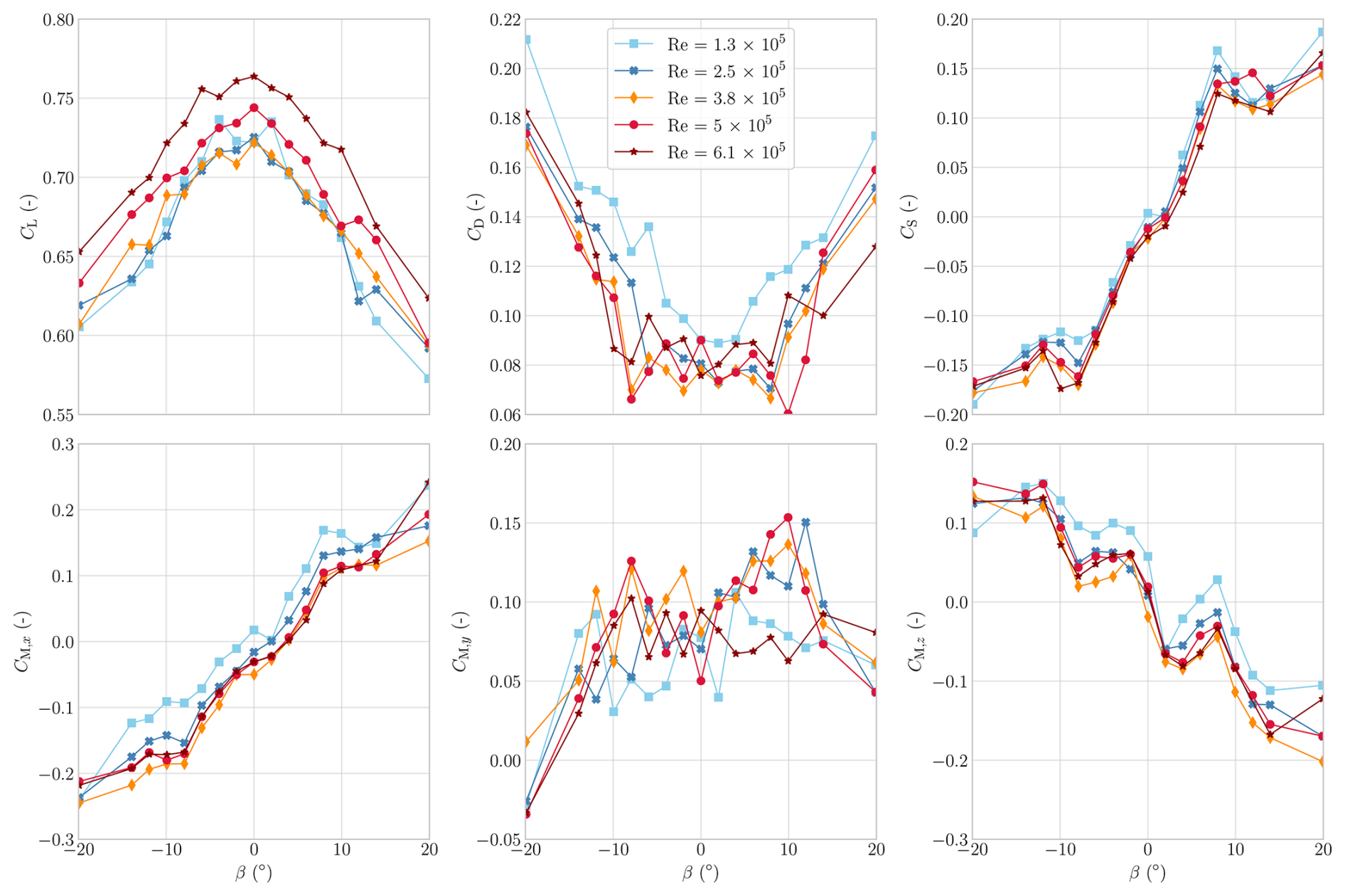
Figure 9 Aerodynamic force and moment coefficients plotted against β for Re varying from 1.3×10⁵ to 6.1×10⁵, at α=7.4°.

The C_L plot reveals an overall increase in lift coefficient with increasing Re, consistent with the findings when varying α. Notably, around β=8°, the C_S curve exhibits both positive and negative peaks, suggesting a nonlinear relationship with β. At this same angle, a local maximum is observed in C_M,x for the $\mathit{\text{Re}}=\mathrm{5}\times {\mathrm{10}}^{\mathrm{5}}$ case, and off-trend behaviour can be seen for C_D and C_M,z. Similar off-trend behaviour near $\mathit{\beta }=\pm \mathrm{8}\mathrm{°}$ also appears in β sweeps at other values of α. The potential underlying causes of this phenomenon are examined further in Sect. 4.

Among the tested cases with complete measurement sets, $\mathit{\text{Re}}=\mathrm{5}\times {\mathrm{10}}^{\mathrm{5}}$ represents the highest Reynolds number and is therefore the closest to actual in-flight operational conditions, which is around $\mathit{\text{Re}}=\mathrm{3}\times {\mathrm{10}}^{\mathrm{6}}$ (Cayon et al., 2025). Consequently, this case is used as the basis for comparison with the numerical simulations. Additional arguments for choosing this specific measurement run are the low measurement uncertainty, as indicated by the CV_i values in Table 3; its high repeatability, demonstrated in Table 4; and the high degree of symmetry and antisymmetry in the positive and negative β measurements.

4 Discussion

Since the primary objective of the wind tunnel campaign was to generate validation data for numerical models, the measured aerodynamic characteristics were compared to characteristics obtained from several different aerodynamic computational studies of the V3 kite. One suitable data source is the Reynolds-averaged Navier–Stokes (RANS) CFD analysis by Viré et al. (2022), which is also the origin of the surface geometry employed in the present study. The closest corresponding simulation case in terms of Reynolds number is at $\mathit{\text{Re}}=\mathrm{10}\times {\mathrm{10}}^{\mathrm{5}}$, for which force data are available from both an α sweep at β=0° and a β sweep at α=13.02°. The reported C_S values differ from those presented by Viré et al. (2022), as they were corrected by a factor of 3.7. This correction factor corresponds to the ratio of the projected side area used by Viré et al. (2022) to the planform area A adopted in the present study. It was applied to enable consistent comparison between the aerodynamic force and moment coefficients. Since RANS CFD is generally considered unsuitable for accurate modelling of unsteady separated flows (Speziale, 1998), the post-stall residuals were examined to assess the validity of the solution. Compared to the pre-stall cases, the post-stall results exhibited larger residuals, with values ranging from $\mathrm{1.0}\times {\mathrm{10}}^{-\mathrm{5}}$ to $\mathrm{2.2}\times {\mathrm{10}}^{-\mathrm{5}}$, rather than remaining below $\mathrm{1.0}\times {\mathrm{10}}^{-\mathrm{6}}$ as observed in pre-stall conditions. Nevertheless, these data points were retained in the analysis due to their relevance to the overall aerodynamic behaviour.

A second data source is the RANS CFD analysis by Viré et al. (2020) of the same wing but without struts. This study provides force data over an α sweep at $\mathit{\text{Re}}=\mathrm{5}\times {\mathrm{10}}^{\mathrm{5}}$. As shown by Viré et al. (2022), the struts have only a negligible impact on the integral force coefficients of the 3D wing. For both CFD datasets from Viré et al. (2020, 2022), it was determined that the geometry file contained a 1.02° offset in the angle of attack, defined as the angle between the mid-span chord line and the apparent wind vector. Therefore, the numerical data presented here were corrected by applying this angle of attack offset; further details are provided in Appendix F.

The third computational dataset was generated in the present study using a vortex-step method (VSM), which is a lifting-line type of method. The VSM code, originally developed by Cayon et al. (2023), was adapted for the present comparisons; for details, see Poland et al. (2026). For each simulation, the angle of attack was incremented in steps of 1°, and a convergence analysis confirmed that discretizing the wing into 150 spanwise panels was sufficient. The VSM relies on 2D airfoil polars as input. In previous studies, these polars were constructed using aerodynamic load correlations derived from a large set of CFD simulations (Breukels, 2011). In the present work, however, more accurate polars are employed, obtained from dedicated 2D RANS CFD simulations; the differences and simulation setup are discussed in detail in Poland et al. (2026).

To ensure that the numerical tools accurately represent real-world flight conditions, it is essential to characterize the range of inflow angles encountered during kite operation. In-flight measurements (Schelbergen et al., 2024) were analysed by Cayon et al. (2025), who found that the angle of attack α of the 3D wing averaged around 1° during the reel-in phase and approximately 8° during the reel-out phase. Additionally, observed sideslip angles β typically range between −10 and 10° (Oehler et al., 2018). The forthcoming comparison of simulations and measurements should be interpreted in light of these respective operating ranges and differences in canopy thickness; specifically, the scale model featured a thicker canopy, which may have contributed to increased drag and lift.

4.1 Force comparison

In Fig. 10, the force coefficients C_L, C_D, and $L/D$ are plotted against α for the VSM, CFD, and wind tunnel (WT) data, along with 99 % CI bands, evaluated using the autocorrelation-consistent method by Newey and West (1987). The CI band is rather narrow for C_L compared to the mean values, indicating high certainty. For C_D, the band is wider, aligning with the difference in the CV listed in Table 3. The numerical data match the measured lift coefficient trend well from $\mathit{\alpha }=-\mathrm{11}$ to around 11°. Above α=11°, the numerical VSM predicts lower lift, whereas the RANS CFD predicts substantially higher lift. The differences in numerical predictions around stall are considered to arise, in part, from discrepancies in turbulence modelling. The VSM employs fully turbulent 2D RANS CFD as input, whereas the 3D RANS CFD simulations both incorporate a transition model (Viré et al., 2020, 2022).

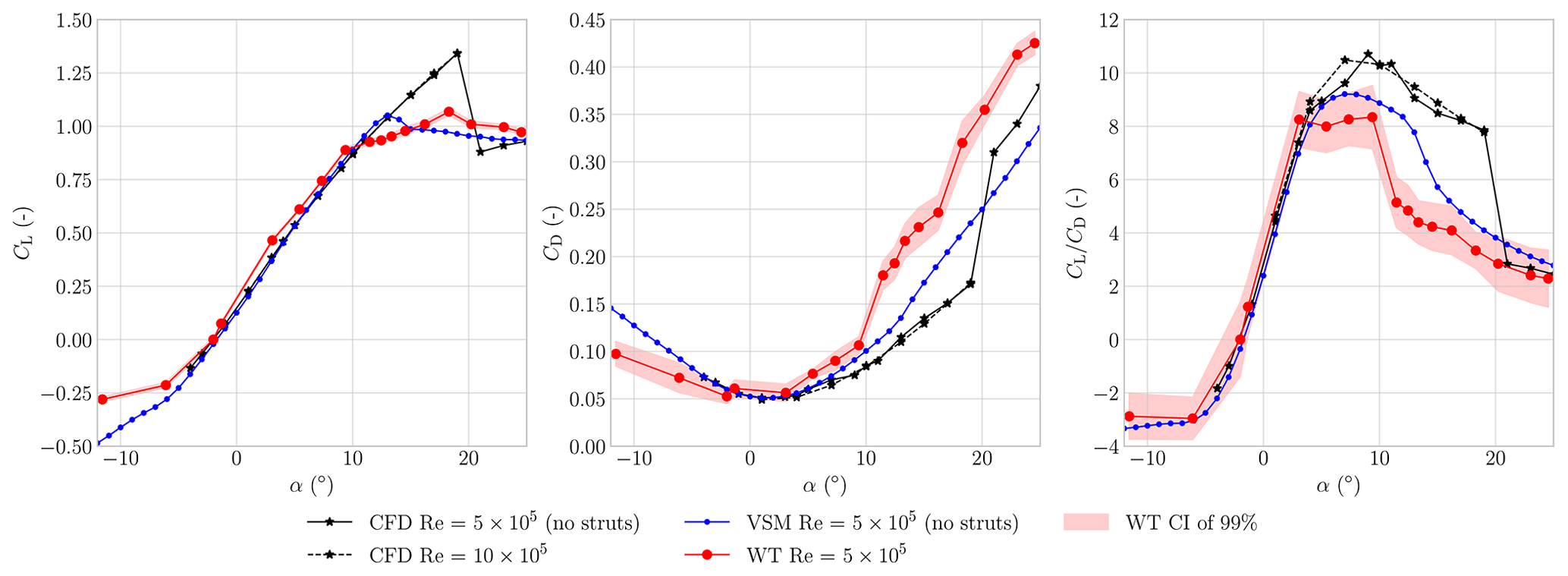
Figure 10 Measured lift and drag coefficients and their ratio, together with coefficients computed with VSM and RANS CFD (Viré et al., 2020, 2022), plotted against α at β=0°.

The numerical and measured drag coefficients start deviating more above around α=10°, where the lift slope also changes. Both VSM and CFD predictions with and without struts agree well but do not show the same expected change in drag slope when entering the stall regime. The change of slope is not reproduced by the VSM predictions to the same extent, attributed to inherent limitations of lifting-line-based methods in this regime (Phillips and Snyder, 2000), e.g. its inviscid nature.

From α=1 to 10°, the measured lift-to-drag ratio plateaus at the maximum value range between $L/D=\mathrm{8}$ and 8.5, sharply dropping outside this α range. All numerical models predict a higher maximum $L/D$: the CFD simulations reach a value of 10.5, while the VSM predicts a maximum of 9.5.

In Fig. 11, the force coefficients C_L, C_D, and C_S are plotted against β for α=12.5°. CFD data were only available at a different angle of attack, α=13.02°, but is included regardless to enable trend comparison. Furthermore, the WT data are plotted for both positive and negative β ranges to illustrate the effect of the asymmetric measurement setup, e.g. due to geometry, surface condition, or inflow.

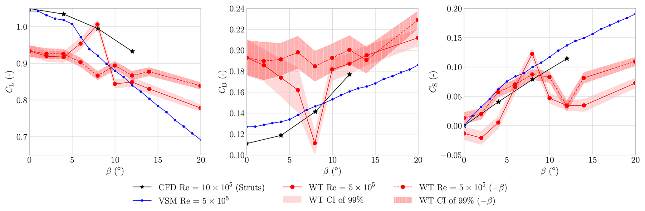
Figure 11 Measured lift, drag, and side force coefficients, together with coefficients computed with VSM and RANS CFD (Viré et al., 2022), plotted against β, for α=12.5°.

The measurements confirm and closely follow the trends predicted by the numerical simulations. With increasing sideslip angle, C_L decreases, while C_D and the absolute value of C_S increase. The measured data at negative β form an exception, showing an off-trend lift, drag, and side force behaviour above around β=8°. This off-trend behaviour appears across multiple Re values, as shown in Fig. 9, and is smaller for the lower-α case. Since this behaviour was not observed in the CFD or VSM predictions, and as an increase in lift and side force and a decrease in drag were measured, it suggests the presence of local separated flow in the positive β case and attached flow in the negative β case. These differences are attributed to asymmetry in the measurement setup and surface imperfections on the scale model.

4.2 Moment comparison

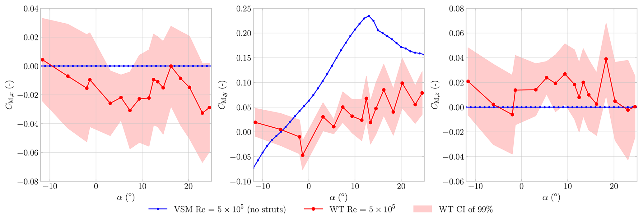
The moment coefficients C_M,x, C_M,y, and C_M,z are plotted over an α sweep in Fig. 12. Compared to the force measurements, the confidence intervals are wider due to higher measurement uncertainty, the same conclusion as drawn from analysing CV shown in Table 3. No CFD data are available; therefore, only VSM data are used. The numerical data predict no roll or yaw moment, where the measurements do show, on average, a negative roll moment coefficient C_M,x and a positive yaw moment coefficient C_M,z, indicating asymmetries in the setup. The experimental pitch moment coefficients C_M,y fluctuate significantly, yet on average exhibit a positive slope. The numerical predictions differ in magnitude but exhibit a similar positive and increasing moment trend up to the stall point.

Figure 12 Measured and computed moment coefficients as functions of α at β=0°.

In Fig. 13, the moment coefficients C_M,x, C_M,y, and C_M,z are plotted over a β sweep. Similar to the forces, the measured moments differ between positive and negative β ranges. The numerical and experimental data match well for the roll moment coefficient C_M,x. Less agreement in trend is shown for the pitch moment coefficient C_M,y, where the measurements indicate an increasing moment up to β=10° and above this threshold a decreasing moment. The VSM, on the other hand, predicts a higher value that changes less with increasing β. For the yaw moment coefficient C_M,z, the measurements and numerical predictions show opposite trends; it is unclear why this is the case. The currently measured negative slope suggests that the anhedral kite shape was yaw statically stable, which is identical to the findings of Belloc (2015), where a negative slope was measured for an anhedral rigidized paraglider in wind tunnel experiments. Possible factors contributing to the prediction discrepancy include observed setup asymmetry; high uncertainty, as shown in Table 3; and a low signal-to-noise ratio, as presented in Fig. D1 in Appendix D. Furthermore, because the moments are computed about a prescribed reference point, any mismatch between the centre of gravity definition in the measurements and that used in the simulations would directly affect the predicted moment levels and could therefore contribute to the observed discrepancy.

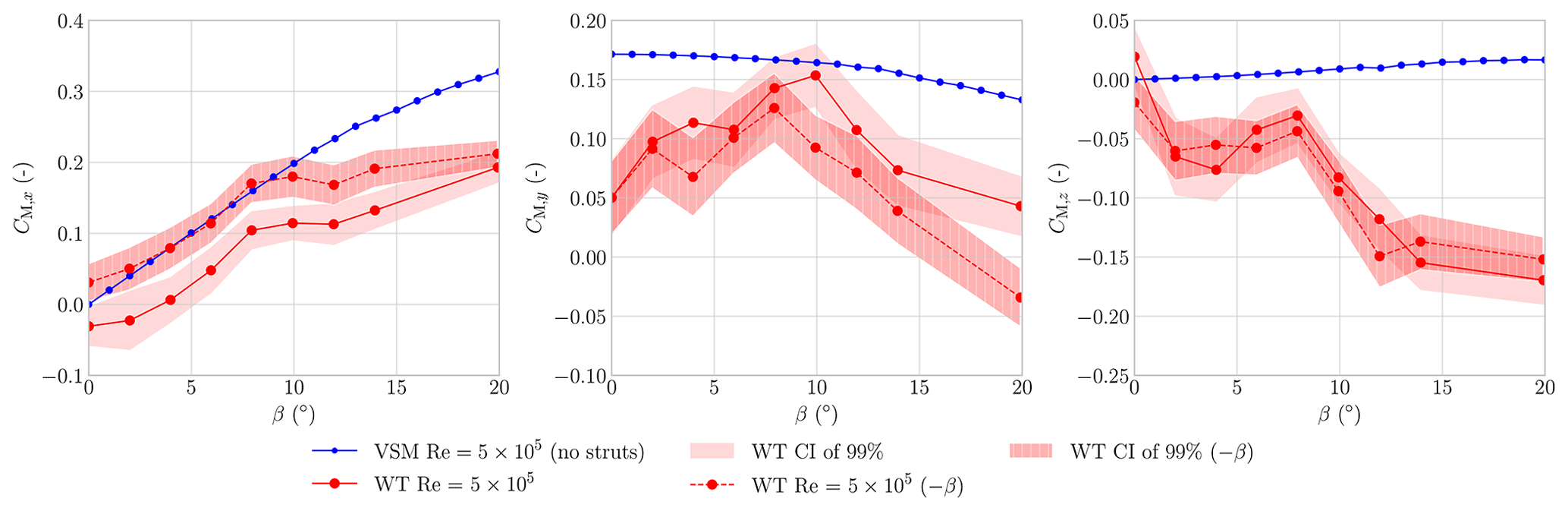
Figure 13 Measured moment coefficients together with coefficients computed with VSM simulations, plotted against β, for α=7.4°.

5 Conclusions

This paper presents a wind tunnel investigation of an LEI kite, designed as a benchmark case to validate numerical models for airborne wind energy applications. To avoid scaling issues caused by aero-structural deformation, a 1:6.5 rigid-scale model of the TU Delft V3 kite was used. The same idealized geometry as that used in the numerical studies, except for a thicker canopy, was employed. The experiments were conducted in the Open Jet Facility at TU Delft, with wind tunnel corrections applied primarily to account for downwash effects.

A zigzag tape was applied to replicate the aerodynamic effect of the stitching seam that connects the canopy to the leading-edge tube. Its height was selected based on theoretical criteria to induce boundary layer transition. At a Reynolds number of 5×10⁵, the addition of the zigzag tape led to a reduction in lift and an increase in drag, aligning with trends reported in the literature. Despite the limited data and kites typically operating at higher Reynolds numbers, the findings suggest that the suction side stitching seam negatively affects the aerodynamic performance.

In the nominal operating regime, the experimental data confirm the lift, drag, and side force predictions made by the VSM simulations conducted in this study, as well as by previously published RANS CFD simulations. Between 0–10° angle of attack, the lift-to-drag ratio remains nearly constant, between 8–8.5. This behaviour deviates from conventional wing aerodynamics and warrants careful consideration in kite simulations, as current numerical models are unable to capture the nearly constant trend, likely due to an underestimation of drag in the relevant flow regime. The remaining differences are attributed primarily to possible misprediction of the flow behind the circular leading-edge tube and to the simulation of a canopy with reduced thickness.

Within the nominal sideslip range, from −10 to 10°, the experimental results confirm the numerical side force predictions. Given that sideslip conditions inherently arise during turning manoeuvers and that side force plays a critical role in initiating and sustaining such motions, the observed agreement suggests that there is aerodynamic potential within the presented numerical models for accurately predicting steering behaviour.

The measurements and simulations differed the most outside the nominal angle of attack and sideslip operating ranges. This discrepancy is partly attributed to differences between the wind tunnel conditions and the simulated environment but also due to the decreasing accuracy of the employed numerical predictions beyond the onset of stall. While the discrepancies indicate potential areas for model refinement, they are not inherently detrimental to accurately predicting kite aerodynamic loads, as they primarily occur outside the nominal operating envelope.

Although this study provides a rigorous evaluation and benchmarking of numerical models through direct comparison with carefully acquired experimental data, the simulations are not yet considered fully validated. Strict validation would require a comprehensive assessment across multiple geometries, operating conditions, and Reynolds numbers, as well as the resolution of the identified limitations to ensure reliable predictive capability across the full operational envelope.

The reported measured values will differ from those of a real kite, as an idealized shape was analysed. The actual kite geometry, lacking edge fillets and incorporating a bridle line system, will likely exhibit higher drag. Furthermore, structural deformations such as canopy billowing and unsteady aerodynamic loads will further alter the aerodynamic response.

Future work should investigate the causes of the measured asymmetry and aim to reduce uncertainty in moment measurements. To study transition and the influence of the stitching seam in more detail, more refined measurement techniques, e.g. infrared thermography, are recommended. For improved numerical validation, CFD simulations should be conducted at all measured Reynolds numbers and inflow angles, including moment predictions and the full experimental setup, the latter to confirm the applied corrections. A particle image velocimetry study has already been conducted to analyse the flow fields and enhance understanding; the paper is published as a companion paper (Poland et al., 2025a).

Appendix A: Statistical convergence of measurement period

A measurement duration of 10 s was selected based on the characteristic aerodynamic timescale of the system, defined as the time required for a fluid element to traverse the kite's reference chord. For each tested condition, this corresponded to approximately 125–625 independent flow passages within the 10 s interval, depending on the free-stream velocity. This ensured that statistical averages were derived from a sufficiently large number of uncorrelated samples, thereby mitigating the influence of temporally correlated fluctuations.

To assess statistical convergence, key measurement conditions – namely α=5.7° at U=20 m s⁻¹ and $\mathit{\beta }=-\mathrm{20}$, 0, and 20° – were repeated three times. The close agreement in both mean and fluctuating load coefficients across these repetitions confirmed that a 10 s sampling window was adequate to obtain converged statistics under the present steady-state aerodynamic conditions. While longer sampling durations may be necessary for capturing slower or rare unsteady phenomena, the selected interval was found to be appropriate for the regime investigated.

To further substantiate this, a convergence analysis was performed using both running average and block analysis techniques. As shown in Fig. A1, these methods revealed only marginal fluctuations in the computed statistics over the 10 s window, thereby validating the statistical robustness of the chosen measurement duration.

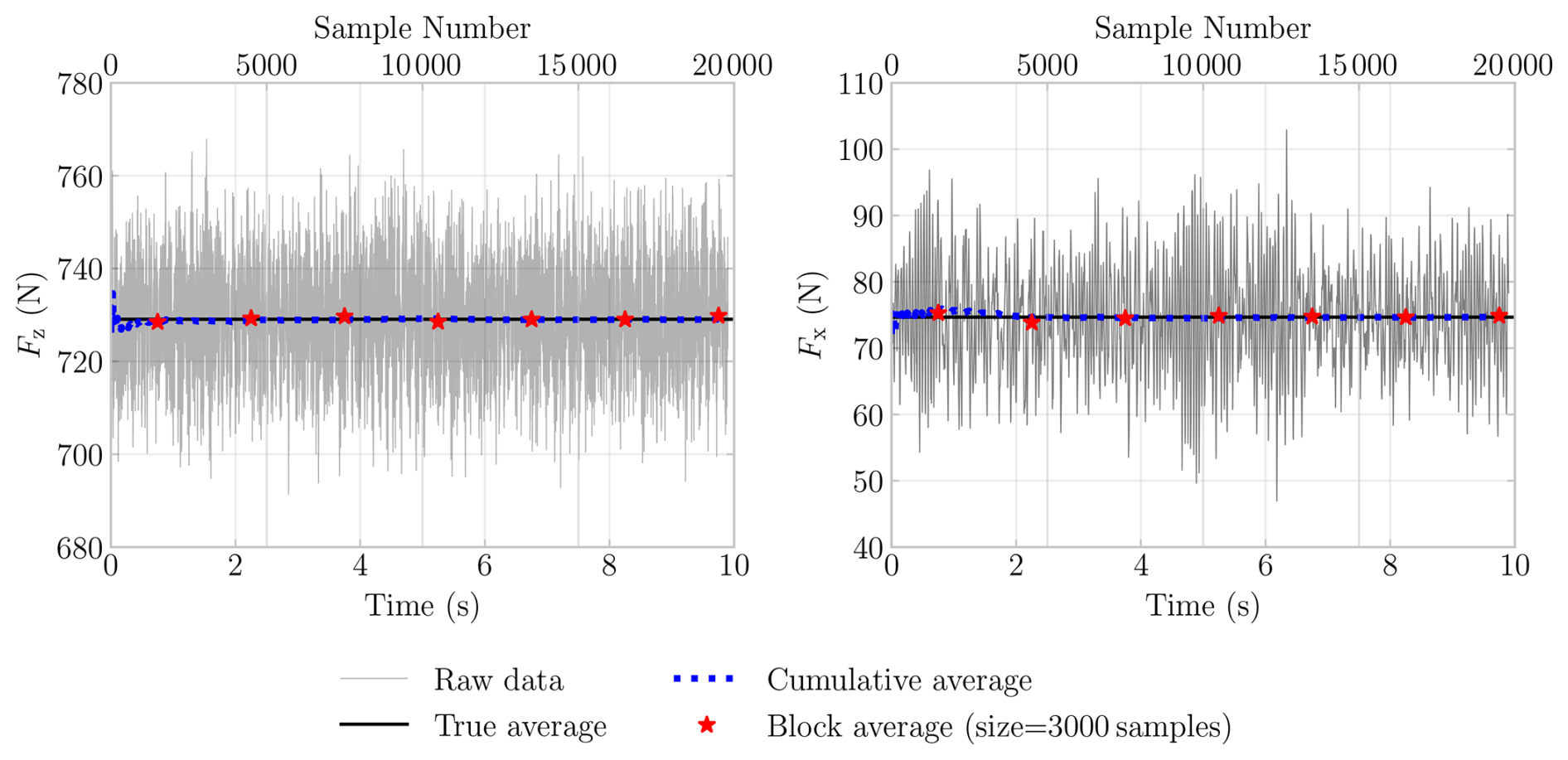
Figure A1 Running average and block average analyses of the 10 s over a sample showing the forces in the z and x axes, demonstrating that the selected period is sufficiently long to achieve a statistically converged average.

Appendix B: Wind tunnel corrections

B1 Wind tunnel blockage

Two different effects contribute to the blockage of the flow in the wind tunnel, both affecting the dynamic pressure. There is solid blockage due to the frontal area of the wing and wake blockage arising from momentum loss in the wake downstream of the model. One can estimate the total blockage using the blockage factor, defined as the ratio between the model's frontal area and the jet exit's cross-sectional area (Mercker et al., 1997). With the kite set at the maximum tested angle of attack of 24°, the projected frontal area A_f at α=24° is approximately 0.2 m². The octagonal wind tunnel opening has an area S_n=7.47 m², resulting in a blockage factor of 3 %. For blockage factors below 10 %, the open-jet wind tunnel correction model of Lock (1929) has been validated against CFD simulations (Collin, 2019), which states

$$\begin{array}{}\text{(B1)}& {\displaystyle }{\displaystyle \frac{\mathrm{\Delta }U}{U_{\mathrm{\infty }}}}=\mathit{\tau }\mathit{\lambda }{\left({\displaystyle \frac{A_{\mathrm{f}}}{S_{\mathrm{n}}}}\right)}^{\frac{\mathrm{3}}{\mathrm{2}}},\end{array}$$

where τ represents the tunnel shape factor of approximately 0.22, and λ is the model shape factor of approximately 0.7, both calculated using the length-to-thickness ratio c_ref and h. The resulting velocity correction is approximately 0.25 %.

Barlow et al. (1999) present another approximation form of the total blockage,

$$\begin{array}{}\text{(B2)}& {\displaystyle }{\displaystyle }{\mathit{ϵ}}_{\mathrm{t}}\approx {\displaystyle \frac{A_{\mathrm{f}}}{\mathrm{4}{S}_{\mathrm{n}}}},\end{array}$$

with which one finds a correction of 0.67 %.

As both methods result in values below 1 %, the blockage effects are considered negligible. This aligns with the guidelines of Wickern (2014), which recommend keeping blockage factors below 5 %, and Barlow et al. (1999), which advise a maximum of 7.5 %.

B2 Streamline curvature and downwash

The correction model described by Barlow et al. (1999) was used. Although not explicitly stated, it was likely developed for conventional planar wings. The swept-back, highly curved anhedral kite wing is non-planar. In the absence of open-jet tunnel corrections that take dihedral effects into account, the model was assumed valid.

Barlow et al. (1999) define the total angle correction as the sum of a downwash correction Δα and a streamline curvature correction Δα_sc in rad:

$$\begin{array}{}\text{(B3)}& {\displaystyle }{\displaystyle }\mathrm{\Delta }{\mathit{\alpha }}_{\mathrm{t}}=\mathrm{\Delta }\mathit{\alpha }+\mathrm{\Delta }{\mathit{\alpha }}_{\text{sc}}.\end{array}$$

B2.1 Downwash

The downwash angle correction Δα in rad is calculated using

$$\begin{array}{}\text{(B4)}& {\displaystyle }{\displaystyle }\mathrm{\Delta }\mathit{\alpha }=\mathit{\delta }{\displaystyle \frac{A}{C}}{C}_{\mathrm{L}},\end{array}$$

where A=0.462 m² represents the model reference area by which the model lift coefficient, C_L, is defined. The octagonal tunnel jet-exhaust cross-sectional area is C=7.47 m². The variable δ represents an empirically determined factor, given by Barlow et al. (1999) as a function of the wind tunnel geometry and the effective vortex span b_e. b_e≈0.79 was found using

$$\begin{array}{}\text{(B5)}& {\displaystyle }{\displaystyle }{b}_{\mathrm{e}}={\displaystyle \frac{b}{\mathrm{2}}}\left(\mathrm{1}+{\displaystyle \frac{b_{\mathrm{v}}}{b}}\right),\end{array}$$

where the ratio of the vortex span b_v to geometric span b=1.287 m was found, from Fig. 10.11 on p. 382 in Barlow et al. (1999) using a taper ratio of λ_t≈0.53 and an aspect ratio of ≈3.5.

Assuming a near-elliptical loading, the δ for an octagonal jet can be approximated using the empirical relations of an open circular-arc wind tunnel (Rosenhead, 1933; Batchelor, 1944). With a ratio of minor to major jet axes λ=1, and the ratio of effective span to jet height k≈0.4, $\mathit{\delta }\approx -\mathrm{0.126}$ was determined from Fig. 10.126 on p. 393 in Barlow et al. (1999).

B2.2 Streamline curvature

The streamline curvature angle correction Δα_sc in rad is related to the downwash angle correction

$$\begin{array}{}\text{(B6)}& {\displaystyle }{\displaystyle }\mathrm{\Delta }{\mathit{\alpha }}_{\text{sc}}={\mathit{\tau }}_{\mathrm{2}}\mathrm{\Delta }\mathit{\alpha },\end{array}$$

where τ₂ is an empirically determined factor dependent on whether the wind tunnel has an open or closed test section and the ratio between tail length l_t and tunnel width 2R=2.85 m. Barlow et al. (1999) state that, for wings without a defined tail length, one can use a quarter of the chord length instead of the tail length, resulting in l_t≈0.10 m. With a ratio of 0.035, one finds from Barlow et al. (1999, Fig. 10.37 on p. 400) τ₂≈0.054. Because the streamline curvature angle correction has a magnitude of roughly 5.4 % of the downwash angle correction, it is clear that the downwash correction dominates.

B3 Total correction

Rewriting the equations and converting from rad to deg, the total angle and load corrections become

$$\begin{array}{}\text{(B7)}& {\displaystyle }& {\displaystyle }\mathrm{\Delta }{\mathit{\alpha }}_{\mathrm{t}}=(\mathrm{1}+{\mathit{\tau }}_{\mathrm{2}})\mathit{\delta }{\displaystyle \frac{A}{C}}{C}_{\mathrm{L}}{\displaystyle \frac{\mathrm{180}}{\mathit{\pi }}},\text{(B8)}& {\displaystyle }& {\displaystyle }\mathrm{\Delta }{C}_{\mathrm{D}}=\mathit{\delta }{\displaystyle \frac{A}{C}}{C}_{\mathrm{L}}^{\mathrm{2}},\text{(B9)}& {\displaystyle }& {\displaystyle }\mathrm{\Delta }{C}_{\mathrm{L}}=-\mathrm{\Delta }{\mathit{\alpha }}_{\text{sc}}{\displaystyle \frac{\mathrm{d}{C}_{\mathrm{L}}}{\mathrm{d}\mathit{\alpha }}},\text{(B10)}& {\displaystyle }& {\displaystyle }\mathrm{\Delta }{C}_{\mathrm{M},y}=+\mathrm{0.125}\mathrm{\Delta }{\mathit{\alpha }}_{\text{sc}\left(\mathrm{2}\right)}{\displaystyle \frac{\mathrm{d}{C}_{\mathrm{L}}}{\mathrm{d}\mathit{\alpha }}},\end{array}$$

where Δα_sc(2) denotes the streamline curvature correction computed using an l_t equal to half the chord length τ₂₍₂₎≈0.108. A value of $\frac{\mathrm{d}{C}_{\mathrm{L}}}{\mathrm{d}\mathit{\alpha }}\approx \mathrm{0.1}$ was derived from the experimental results.

Barlow et al. (1999) do not mention any application of their corrections towards the sideways y direction. As the kite, under non-zero sideslip conditions, does produce a non-negligible side force, i.e. roughly 15 % of the maximum lift, a downwash and curvature effect might be present. To quantify the effects, it is assumed that the method of Barlow et al. (1999) also holds for the sideways direction in the following form:

$$\begin{array}{}\text{(B11)}& {\displaystyle }& {\displaystyle }\mathrm{\Delta }{\mathit{\beta }}_{\mathrm{t}}=(\mathrm{1}+{\mathit{\tau }}_{\mathrm{2},\mathrm{s}})\mathit{\delta }{\displaystyle \frac{A}{C}}{C}_{\mathrm{S}}{\displaystyle \frac{\mathrm{180}}{\mathit{\pi }}},\text{(B12)}& {\displaystyle }& {\displaystyle }\mathrm{\Delta }{C}_{\mathrm{D}}=\mathit{\delta }{\displaystyle \frac{A}{C}}{C}_{\mathrm{S}}^{\mathrm{2}},\text{(B13)}& {\displaystyle }& {\displaystyle }\mathrm{\Delta }{C}_{\mathrm{S}}=-\mathrm{\Delta }{\mathit{\beta }}_{\text{sc}}{\displaystyle \frac{\mathrm{d}{C}_{\mathrm{S}}}{\mathrm{d}\mathit{\beta }}},\text{(B14)}& {\displaystyle }& {\displaystyle }\mathrm{\Delta }{C}_{\mathrm{M},z}=+\mathrm{0.125}\mathrm{\Delta }{\mathit{\beta }}_{\text{sc}\left(\mathrm{2}\right)}{\displaystyle \frac{\mathrm{d}{C}_{\mathrm{S}}}{\mathrm{d}\mathit{\beta }}},\end{array}$$

with ${\mathit{\tau }}_{\mathrm{2},\mathrm{s}}\approx \mathrm{0.028}$ and ${\mathit{\tau }}_{\mathrm{2}\left(\mathrm{2}\right),\mathrm{s}}\approx \mathrm{0.056}$ calculated using the tip chord c_t=0.212 m. Because C_S is non-dimensionalized by the same area A, and to enable calculations, it is assumed that the same $\mathit{\delta }\approx -\mathrm{0.126}$ can be used. A value of $\frac{\mathrm{d}{C}_{\mathrm{S}}}{\mathrm{d}\mathit{\beta }}\approx \mathrm{0.01}$ was derived from the experimental results.

Table B1 Corrections for angle, force, and moment coefficients.

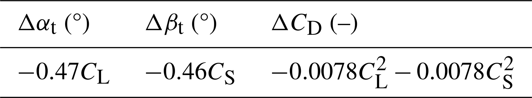
The resulting corrections, similar to the blockage corrections, are deemed negligible if they induce less than 1 % change at their maximum, e.g. a 0.1° change at 10° angle. This renders the ΔC_L, ΔC_M,y, ΔC_S, and ΔC_M,z corrections negligible. An exception is Δβ_t, which does not cause 1 % change but comes close, e.g. taking the case of Fig. 11 one finds for C_S≈0.1 a correction of Δβ_t≈0.046°, which, given β≈10°, implies a 0.46 % change.

Appendix C: Assessment of sensor drift

To ensure consistent data from the load balance measurement device, described in Sect. 2.3 and shown in Fig. 2, sensor drift was evaluated through repeated measurements. Specifically, 30 s time interval measurements were taken each morning and evening over 3 consecutive days, corresponding to 12 h intervals. This procedure served to determine whether the drift was substantial enough to influence the results. The measurement drift over time is plotted in Fig. C1, with corresponding mean and standard deviation values reported in Table C1. On average, the standard deviation across the six components (three translational and three rotational) was approximately 1 N. During the experiment, a baseline measurement at near-zero wind speed was taken after each change in α, followed immediately by a measurement at non-zero U_∞. The aerodynamic load was then obtained by subtracting the baseline from the flow-on measurement. Consequently, sensor drift only affects the resulting data if drift magnitudes occurring over the short interval between the two measurements are comparable to those observed over the 12 h drift assessment intervals.

Table C1 Sensor drift mean and standard deviation σ values.

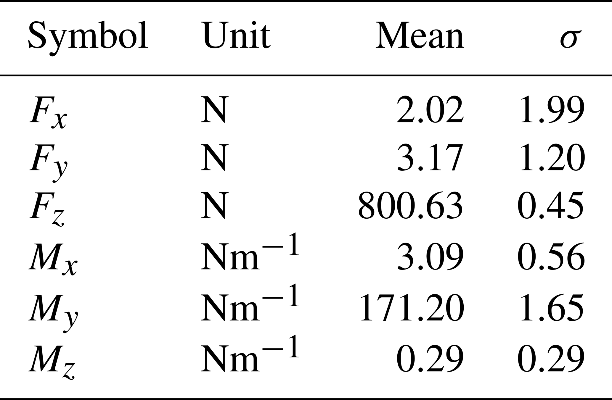
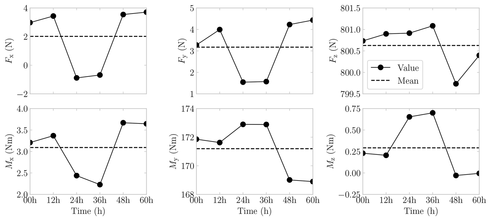
Figure C1 Sensor drift of the load balance for the three force components and three moments during the 60 h measurement time.

Appendix D: Support-structure loads

To illustrate the relative contribution of the kite and support structure to the total measured loads, the proportions of the measured kite loads and support-structure loads are shown in Fig. D1 for a representative case at $\mathit{\text{Re}}=\mathrm{5}\times {\mathrm{10}}^{\mathrm{5}}$ over a β sweep; see Appendix D. Defining the kite load as the signal and the support-structure load as the noise, this ratio serves as a proxy for the signal-to-noise ratio (SNR) and, thus, for measurement uncertainty.

The kite contribution dominates for C_L, indicating a high SNR and low associated uncertainty. In contrast, for C_D, C_M,y, and C_M,z, the support-structure contributions are more significant, implying a lower SNR and correspondingly higher uncertainty.

For proportions in other cases, the reader is referred to the open-source code and open-access dataset, which allow the reproduction of these plots.

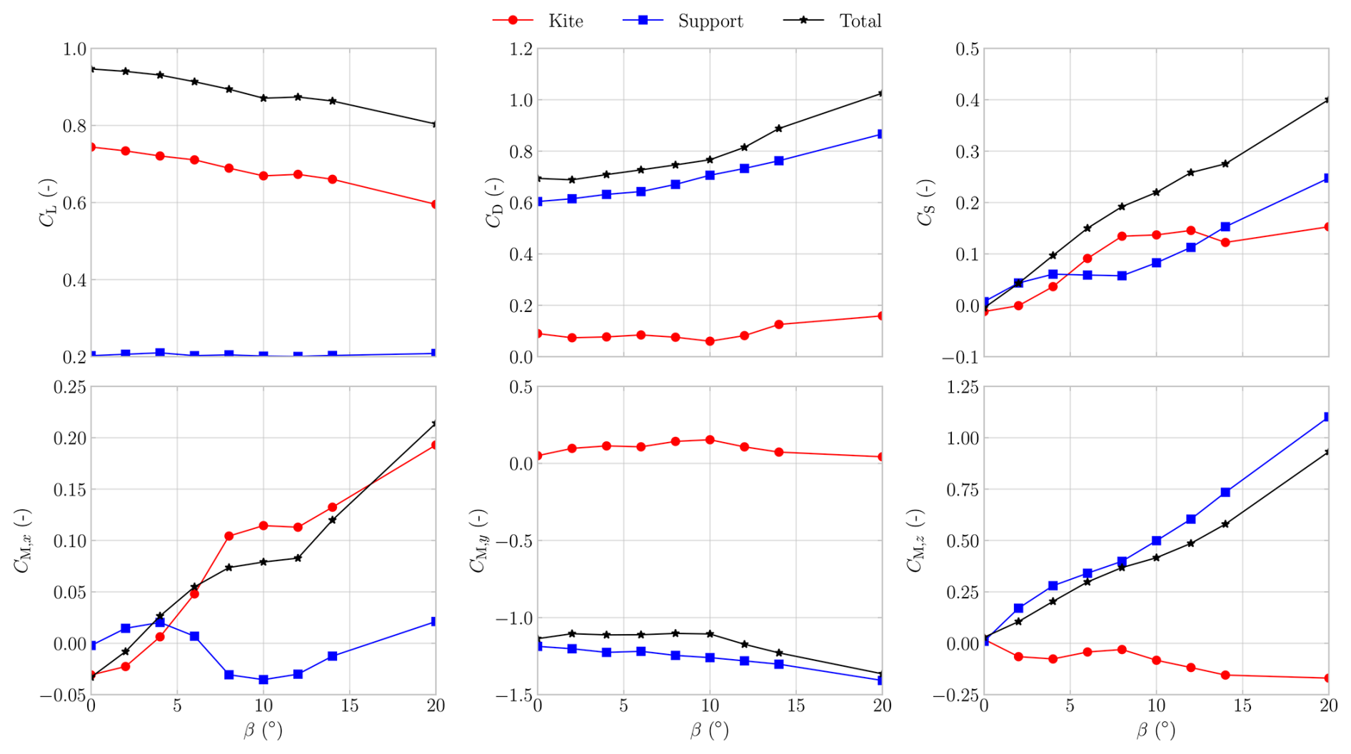
Figure D1 Total measured, support-structure-measured, and kite-measured loads plotted for $\mathit{\text{Re}}=\mathrm{5}\times {\mathrm{10}}^{\mathrm{5}}$ over a positive β sweep for α=7.4°.

Appendix E: Experimental setup vibration analysis

During the measurements, vibrations were observed and analysed both qualitatively from video footage and quantitatively using force and moment data sampled at 2000 Hz; see Fig. E1. At $\mathit{\text{Re}}=\mathrm{6.1}\times {\mathrm{10}}^{\mathrm{5}}$, the vibrations were deemed potentially destructive under high α and high β; therefore, some of the intended experiments were not completed. The increasing vibration amplitudes suggest that a natural frequency of the structure or one of its sub-structures was excited, indicating resonance.

As an example, a 1 s data segment at U_∞=25 m s⁻¹, α=14°, and β=0° is shown in Fig. E1, where the force data exhibit high-frequency oscillations, most notably in F_z, and the moment data display a resonant trend.

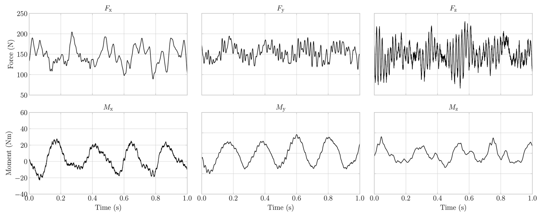
Figure E1 Raw measured values at 2000 Hz by the load balance, over a 1 s period taken at 25 m s⁻¹ with α=15° and β=0°.

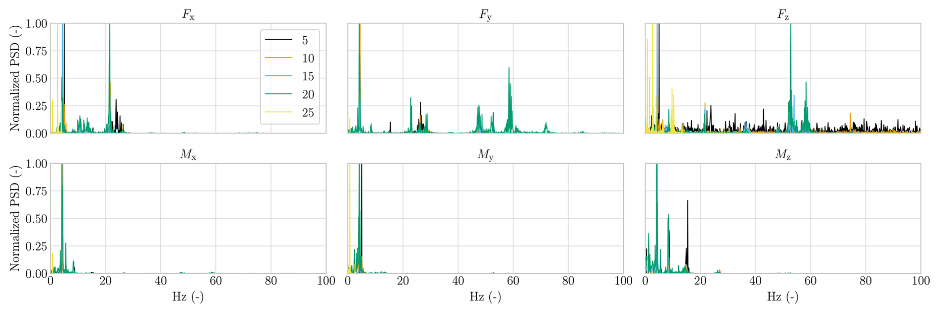
Figure E2 Raw measurements transformed into PSD using FFT and a periodogram function and displayed for the three force and moment components up to 100 Hz.

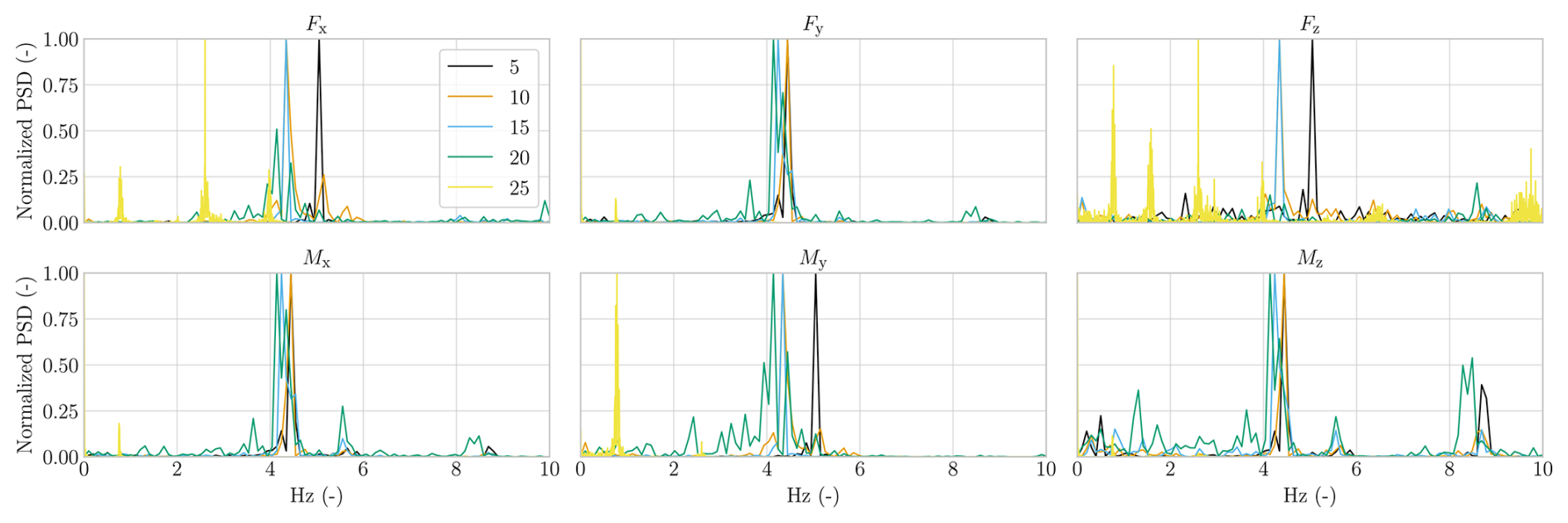
Figure E3 Raw measurements transformed into PSD using FFT and a periodogram function and displayed for the three force and moment components up to 10 Hz.

To investigate the resonance behaviour observed during testing, the time series data were transformed into the frequency domain using a fast Fourier transform (FFT), and the power spectral density (PSD) was computed using a periodogram function. The resulting PSD values were normalized to the range [0, 1] to enable comparison across different wind speeds. For each wind speed, frequency and normalized PSD values were computed for all six channels: three force components (F_x, F_y, F_z) and three moment components (M_x, M_y, M_z).

To examine the influence of wind speed on the frequency content and to identify potential resonance behaviour, the normalized PSDs were plotted up to 100 Hz; see Fig. E2. This frequency range was chosen as the PSD values beyond 100 Hz are negligible in all channels except F_z. As most PSD peaks are concentrated at lower frequencies, the data were also plotted up to 10 Hz; see Fig. E3.

At U_∞=25 m s⁻¹, the number and magnitude of PSD peaks increased, indicating the presence of multiple vibrational modes and aligning with qualitative observations of stronger vibrations. Potential sources of the observed vibrations include structural resonance, wherein the natural frequencies of the experimental setup are excited by unsteady aerodynamic loads, and vortex shedding from the model or its mounting components, which can introduce periodic forcing. Both mechanisms are known to amplify dynamic responses in wind tunnel experiments, particularly at elevated angles of attack and higher wind speeds. Across most components and flow conditions, a dominant peak was consistently observed at 4–5 Hz, corresponding to the natural frequency of the supporting blue table onto which the setup was mounted; see Fig. 2 (LeBlanc and Ferreira, 2018). The alignment of these peaks with the structural resonance frequency confirms the occurrence of resonance and explains the elevated uncertainties observed at high α and β. To avoid introducing filtering-related artefacts and to remain conservative on the uncertainty, it was decided not to filter out the 4–5 Hz band.

Appendix F: Angle of attack offset correction

An offset of 1.02° in the angle of attack was identified in the original V3 kite CAD geometry. This offset originated from a geometric inconsistency: the vector from the mid-span leading edge to trailing edge was tilted upward by 1.02° relative to the intended horizontal reference plane, as shown in Fig. F1. All subsequent simulations in this work were corrected by applying this offset to maintain alignment with the conventional aerodynamic reference frame.

This misalignment was inadvertently propagated into earlier RANS CFD studies, including those by Viré et al. (2020) and Viré et al. (2022). As a result, the angles of attack reported in those publications do not strictly adhere to the standard aerodynamic definition, namely the angle between the incoming flow and the chord line.

The issue was discovered during the present wind tunnel campaign. In subsequent discussions with G. Lebesque – whose MSc thesis formed the basis of Viré et al. (2022) – it was confirmed that the offset had gone unnoticed at the time. This was further substantiated through cross-sectional geometric inspection, where lines connecting the leading and trailing edges showed a clear tilt relative to a horizontal reference; see Fig. F1.

To resolve this discrepancy, the geometry has been corrected to eliminate the offset. Updated and verified CAD files are now publicly available at https://github.com/awegroup/TUDELFT_V3_KITE (last access: 11 February 2026).

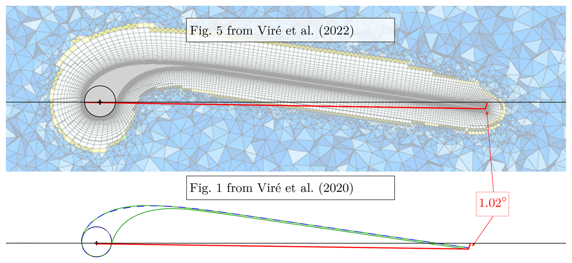
Figure F1 Geometric verification of the angle of attack offset in the original CAD geometry. Each of the three images stacked vertically illustrates the LEI airfoil of the V3 kite at mid-span. The black lines indicate cross-sectional slices through the leading edge, while the red lines represent slices through the trailing edge. The visible vertical mismatch between these lines confirms the presence of the offset.