Wake behavior and control: comparison of LES simulations and wind tunnel measurements

This paper applies a large-eddy actuator line approach to the simulation of wind turbine wakes. In addition to normal operating conditions, a specific focus of the paper is on wake manipulation, which is performed here by derating, yaw misalignment and cyclic pitching of the blades. With the purpose of clarifying the ability of LES methods to represent conditions that are relevant for wind farm control, numerical simulations are compared to experimental observations obtained in a boundary layer wind tunnel with scaled wind turbine models. Results indicate a good overall matching of simulations with experiments. Low-turbulence test cases appear to be more challenging than moderate- and high-turbulence ones due to the need for denser grids to limit numerical diffusion and accurately resolve tip-shed vortices in the near-wake region.

1 Introduction

Wind plants are collections of wind turbines often operating in close proximity of one another. Several complex phenomena take place within a wind farm. First, there is an interaction between the atmospheric boundary layer and the whole wind farm caused by the smaller-scale interaction between the atmospheric flow and each individual wind turbine. Second, within the power plant itself, there is an interaction among upstream and downstream wind turbines through their wakes. In turn, the wakes themselves interact with the atmospheric flow and other wakes, playing a central role in determining the overall behavior of the plant. Wakes produced by upstream wind turbines may have a profound influence on the performance of downstream operating machines. In fact, waked turbines experience lower power output and increased loading compared to clean isolated conditions. A thorough understanding of these complex phenomena is clearly indispensable for optimizing the layout and operation of wind plants. However, even an optimal layout will still incur negative effects due to wake interactions, at least in some wind and environmental conditions. To mitigate these effects, a number of control strategies are currently being investigated to optimize the operation of wind power plants, including power derating, wake deflection and enhanced wake recovery (Fleming et al., 2014; Knudsen et al., 2015).

The current research in this field is very active, covering a broad spectrum that ranges from high-fidelity numerical simulations to reduced order models, from scaled experiments in the wind tunnel to direct measurements in the field, all the way to control methods and various supporting technologies. Among the many studies reported in the literature, meteorological and performance data collected at the Horns Rev and Middelgrunden offshore wind farms have been systematically investigated (Barthelmie et al., 2007; Hansen et al., 2012). Moreover, scaled wind farm experiments were conducted in wind tunnels to study wake deficit and its impact on downstream wind turbines (Medici and Alfredsson, 2006; Chamorro and Porté-Agel, 2009; Bartl et al., 2012). These test campaigns have been actively used to validate several engineering and computational fluid dynamics (CFD) wake models in terms of power capture, velocity profiles and higher-order flow quantities (Barthelmie et al., 2006; Kennedy et al., 2011; Porté-Agel et al., 2011; Gaumond et al., 2014). Wake models can be classified on the basis of their complexity and fidelity to reality. The steady-state kinematic wake model of Jensen (1983) was among the first proposed analytical formulations, later extended by Jiménez et al. (2010) to cover the case of yaw misalignment. Larsen et al. (2007) derived a more sophisticated dynamic wake meandering model. Higher-fidelity models have been developed by using CFD. For example, Carcangiu (2008) used the Reynolds-averaged Navier–Stokes (RANS) equations to simulate near-wake behavior, while Stovall et al. (2010) simulated wind turbine clusters and compared RANS to the higher-fidelity large-eddy simulation (LES) approach. Results indicated that RANS is not sufficiently accurate, as it typically overestimates diffusion.

With the significant increase in computational performance in recent years (thanks to advancements in hardware, software and algorithms), LES has gained an increasing adoption by the wind farm research community (Calaf et al., 2010; Porté-Agel et al., 2011; Churchfield et al., 2012). In fact, LES has the ability to better resolve the relevant flow features, leading to an improved insight on flow characteristics within a wind farm. In addition, several researchers (Jiménez et al., 2010; Fleming et al., 2014; Gebraad et al., 2016) have been using LES to investigate wake control strategies.

Although LES is an approach based on first principles, it is still not completely tuning-free. For example, when used in conjunction with an actuator line method (ALM) to represent wind turbine blades, there is a need to properly tune the procedure used for mapping lifting line aerodynamic forces onto the volumetric grid (Sørensen and Shen, 2002; Martinez et al., 2012). In addition to several algorithmic details, other important characteristics of the simulation are represented by the grid (Jha et al., 2014; Martínez-Tossas et al., 2017) and features of the model, including the presence of nacelle and tower. The effects of the tower have been investigated with different versions of the ALM by Churchfield et al. (2015) and Stevens et al. (2018), with an immersed boundary method by Santoni et al. (2017) and with an actuator surface approach by Yang and Sotiropoulos (2018).

In general, most of the published research focuses on the use of CFD to study wake behavior and control strategies, but pay relatively less attention to the problem of ensuring the fidelity of such simulations to reality. In fact, a comprehensive validation of LES methods for wind turbine wakes is still missing. This is clearly not due to a lack of attention to this problem, but rather to a lack of comprehensive high-quality data sets. Unfortunately, experiments in the field are not without hurdles: in fact, wind conditions cannot be controlled, and measurements at full scale are not always possible or complete. In this sense, testing at scale in a wind tunnel is gaining attention as a means to perform experiments with much more precise knowledge and control of the testing conditions.

As a contribution towards a better understanding of the capabilities and limits of LES for modeling wind turbine wakes, this paper applies a recently developed computational framework to the simulation of scaled wind turbines. These models were operated in a large boundary layer wind tunnel in a variety of conditions. A complete LES-based digital model of the experiments is developed in this work, including a model of the wind tunnel and of the passive generation of sheared and turbulent flows. The paper specifically focuses on operating conditions that are relevant to wind farm control. In fact, the existing literature either uses LES to study wind farm control conditions without comparing simulations against experiments (Jiménez et al., 2010; Fleming et al., 2014, 2015; Gebraad et al., 2016) or considers both numerical and experimental results but not in the context of wind farm control (Jiménez et al., 2010; Lu and Porté-Agel, 2011; Porté-Agel et al., 2011; Wu and Porté-Agel, 2011; Churchfield et al., 2012; Mo et al., 2013; Martínez-Tossas et al., 2015; Sørensen et al., 2015; Nilsson et al., 2015; Shamsoddin and Porté-Agel, 2017; Abkar and Dabiri, 2017; Sedaghatizadeh et al., 2018). The present paper tries to fill this gap by conducting a first preliminary study on the ability of LES to model the behavior of wakes in conditions that are relevant to wind farm control applications. This study is preliminary in the sense that only a limited set of conditions for one isolated wind turbine are analyzed. Wake interactions are analyzed in Wang et al. (2017b, 2018) and in forthcoming publications. The authors believe in the need to clarify to what degree wake modeling methods are indeed able to represent farm-control-relevant conditions, this work being a first limited-scope step in this direction.

The present LES framework is characterized by some distinguishing features. First, the tuning-free immersed boundary (IB) method of Jasak and Rigler (2014) is used to model the effects caused by the nacelle and tower. Second, the integral velocity sampling method (Churchfield et al., 2017) is employed, which reduces the sensitivity of the results – and especially of power – to the mapping of aerodynamic forces onto the fluid flow. Third, an ad hoc developed approach is used for tuning the airfoil polars. In fact, given the small scale of the experimental models, their blades operate at low Reynolds numbers and are therefore designed using special low-Reynolds airfoils. Clearly, the accuracy of the airfoil polars plays an important role in the accuracy of the overall LES simulation. Rotational augmentation, manufacturing imperfections and other effects may influence the behavior of the blade airfoils and alter it with respect to their nominal characteristics, which are typically obtained in 2-D dedicated wind tunnel tests. To address this issue, airfoil polars are tuned here by means of a specific identification method (Bottasso et al., 2014), which makes use of dedicated experimental measurements conducted with the scaled turbine (i.e., not with the single airfoils, but with the rotor on which the airfoils are used). Indeed, the airfoil Reynolds varies depending on the operating condition of the turbine. By accounting for the effects of Reynolds on the airfoil polars, which are particularly relevant at the low Reynolds numbers at which the scaled models operate, better accuracy in the results can be achieved.

The problem of computational cost is addressed in a companion paper (Wang et al., 2018), in which a scale-adaptive simulation (SAS) approach is used to model the unresolved scales, resulting in LES-like behavior at a cost similar to RANS with a roughly similar accuracy.

The paper is organized according to the following plan. The numerical method is described in Sect. 2. The computational setup is reported in Sect. 3, in which a precursor simulation mimicking the process that takes place in the wind tunnel is used for the passive generation of the turbulent flow, whose resulting outflow is used as an inlet for subsequent wind turbine wake simulations (called successor simulations). The experimental setup is presented in Sect. 4, including a short description of the wind tunnel, the scaled wind turbine model and the measurement equipment. Results are discussed in Sect. 5. First, an isolated flow-aligned wind turbine is considered, and the LES framework is tuned to match experimental measurements obtained in this baseline case. Next, the three wake manipulation strategies of derating, yaw misalignment and cyclic pitch control are considered. Here again, low-turbulence experimental results are compared with simulations, without any additional tuning with respect to the parameters chosen in the baseline case. Finally, a moderate-turbulent condition is considered, again without any additional tuning. Conclusions are drawn in Sect. 6.

2 Numerical simulation model

The present LES framework is developed within SOWFA (Churchfield and Lee, 2012; Fleming et al., 2013), a simulation tool based on a standard incompressible solver in the OpenFOAM repository.

The rotor is modeled in terms of actuator lines by direct coupling with the aeroservoelastic simulator FAST (Jonkman and Buhl Jr., 2005). The integral approach of Churchfield et al. (2017) is used to compute the flow conditions at each station along an actuator line and to project the calculated aerodynamic forces back onto the fluid domain using a single Gaussian width value. Aerodynamic forces at each station are computed by interpolating precomputed lift and drag aerodynamic coefficients, which are stored in lookup tables parameterized in terms of angle of attack and Reynolds number. Depending on the problem, the wind turbine model is either controlled in a closed loop by a pitch and torque controller based on the implementation described in Bottasso et al. (2014) or simply by using experimentally measured values of pitch and rotor speed.

Both the constant Smagorinsky (CS) (Deardorff, 1970) and the Lagrangian dynamic Smagorinsky (LDS) (Meneveau et al., 1996) models are implemented. However, results of extensive numerical experiments indicate that, for the present application, the performance of LDS is very similar to CS, as shown later in this work and already observed by Sarlak et al. (2015) and Martínez-Tossas et al. (2018) in turbulent conditions.

The IB formulation of Lai and Peskin (2000), Mittal and Iaccarino (2005), and Jasak and Rigler (2014) is used to model the wind turbine nacelle and tower, whose effects on the flow proved to be quite significant, at least in the near-wake region, and should therefore not be neglected (Wang et al., 2017b). The IB method is employed to avoid the use of surface-conforming meshes to represent the shape of such bodies (Mittal and Iaccarino, 2005). The present IB approach, based on a discrete forcing method, uses a direct imposition of the boundary conditions (Uhlmann, 2005), thus preserving the sharpness of the body shape. Boundary conditions and wall models can be directly imposed on the IB surfaces with this approach, yielding good solution quality for high-Reynolds viscous flows (Bandringa, 2010). Details on the formulation are reported in Wang et al. (2017b).

ALM-modeled blades and an IB-modeled nacelle and tower introduce local numerical dispersion and diffusion, which affect simulation stability and accuracy (Holzmann, 2016; Moukalled et al., 2016). The gamma-bounded high-resolution interpolation method is used here to address this issue (Jasak et al., 1999). The gamma scheme is parameterized in terms of β_m, a tunable constant that allows one to control the level of upwinding. In general, a larger value of β_m implies a lower dispersion and a higher diffusion (i.e., more upwinding) and vice versa. The value β_m=0.45 is employed in the near-wake region to stabilize the simulation, since actuator line body forces and an immersed boundary possibly generate numerical dispersion, and β_m=0.05 is used in the far wake to minimize numerical diffusion while retaining a minimum amount of necessary upwinding.

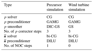
Table 1 shows the linear solvers used for the precursor and the wind turbine–wake simulations. The precursor problem has slightly less regular grids because of the need to mesh the large turbulence generators (termed spires) placed at the tunnel inlet, which requires a slightly different setup of the linear solvers. The PISO time-marching algorithm recursively solves (or corrects) the pressure flux equation to account for non-orthogonal grid elements (Greenshields, 2015). The number of iterations is fixed a priori and set equal to 1 and 0 for the precursor and successor simulations, respectively. Indeed, given the good quality of the grid in the latter case, non-orthogonal corrections are not indispensable, and their elimination lowers the computational cost by about 10 %.

Table 1 Linear algebraic solvers used for the precursor and the wind turbine–wake simulations (CG: conjugate gradient; GAMG: geometric–algebraic multigrid; DIC: diagonal incomplete Cholesky; GS: Gauss–Seidel; DILU: diagonal incomplete LU factorization; NOC: non-orthogonal corrector).

Multi-airfoil table identification

Clearly, the accuracy of the sectional aerodynamic coefficients is a crucial ingredient of the ALM formulation. A method to tune the aerodynamic polars of lifting lines was described in Bottasso et al. (2014). In a nutshell, the method works by first measuring thrust and torque on a rotor at a number of different operating conditions that cover the angles of attack and Reynolds numbers of interest. Next, these values are used to update some given baseline polars by using a maximum-likelihood criterion.

Nominal values of both the lift and drag coefficients C_k (where k=L or k=D for lift and drag, respectively) are corrected as

$$\begin{array}{}\text{(1)}& C_k(\mathit{\eta },\mathit{\alpha },\mathit{\text{Re}})=C_k^{\mathrm{0}}(\mathit{\eta },\mathit{\alpha },\mathit{\text{Re}})+{\mathrm{\Delta }}_k(\mathit{\eta },\mathit{\alpha },\mathit{\text{Re}}),\end{array}$$

where $\mathit{\eta }\in [\mathrm{0},\mathrm{1}]$ is a span-wise location, α the angle of attack, Re the Reynolds number, $C_k^{\mathrm{0}}$ the nominal coefficient value and Δ_k the unknown correction. This latter term is expressed by a linear interpolation as

$$\begin{array}{}\text{(2)}& {\mathrm{\Delta }}_k(\mathit{\eta },\mathit{\alpha },\mathit{\text{Re}})={\mathit{n}}^T(\mathit{\eta },\mathit{\alpha },\mathit{\text{Re}}){\mathit{p}}_k,\end{array}$$

where p_k is the vector of unknown nodal values and $\mathit{n}(\mathit{\eta },\mathit{\alpha },\mathit{\text{Re}})$ is the vector of assumed multi-linear shape functions. To improve the well-posedness of the problem, the polar correction terms are transformed using a singular-value decomposition, which ensures the actual observability of the tuned parameters. Through this method, the corrections to the baseline lift and drag characteristics of the airfoils are recast in terms of a new set of statistically independent parameters. By analyzing their associated singular values, one can retain in the identification only those parameters that are observable with a desired level of confidence (Bottasso et al., 2014).

The unknown correction terms are computed by maximizing the likelihood function of a sample of N available experimental observations. This amounts to first minimizing the following cost function:

$$\begin{array}{}\text{(3)}& J={\displaystyle \frac{\mathrm{1}}{\mathrm{2}}}\sum _i^N{\mathit{r}}_i^T{\mathbf{R}}^{-\mathrm{1}}{\mathit{r}}_i,\end{array}$$

where r is the discrepancy between power and thrust coefficients computed by a blade element momentum model as implemented in the WT-Perf code (Platt and Buhl, 2012) and the corresponding experimentally measured quantities. The optimization is performed for a fixed covariance R by using the gradient-based sequential quadratic programming approach. Next, the covariance is updated as $\mathbf{R}=\mathrm{1}/N{\sum }_i^N{\mathit{r}}_i{\mathit{r}}_i^T$, and the optimization is repeated. Iterations between the minimization and covariance update are continued until convergence (Bottasso et al., 2014).

More than 100 operating points were measured experimentally. The operating conditions were determined in order to cover a desired range of angles of attack and Reynolds numbers, and they were obtained by operating the scaled wind turbine model at different tip speed ratios (TSRs) and blade pitch angles. Experiments were then grouped in terms of average blade Reynolds number, and for each group a separate identification was performed, yielding a calibrated version of the polars at that specific Reynolds.

3 Computational setup

3.1 Precursor simulation

The LES-ALM numerical model was used to create a complete digital copy of the experiments, which were conducted in the 36 m × 13.84 m × 3.84 m boundary layer test section of the wind tunnel at Politecnico di Milano (Zasso et al., 2005; Bottasso et al., 2014).

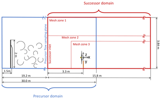
A first simulation is used to generate the turbulent inflow (precursor) used as an inlet for successive wind turbine–wake (successor) simulations. The layout of the partially overlapped precursor and successor domains is represented in Fig. 1. The precursor domain has a size of 30 m × 6.92 m × 3.84 m. The reduced width of the domain with respect to the actual tunnel size is chosen to limit the computational cost. The turbulent inflow for the successor simulation is sampled 19.2 m downstream of the precursor inlet, as shown in the figure. The simulation mimics the passive turbulence-generating system adopted in this wind tunnel (Zasso et al., 2005). A structured body-conforming mesh discretizes the volume around the turbulence-generating spires at the wind tunnel inlet using a purely hexahedral O grid. The average stretching ratio for the volume mesh is 1.25, while the maximum skewness is equal to 2.7, which does not compromise the simulation stability. Mesh quality is limited by the sharp edges and abrupt surface changes in the spire geometry.

Figure 1 Layout of the partially overlapped precursor and successor computational domains.

Dirichlet-type nonslip conditions are used for the resolved velocity vector $\stackrel{\mathrm{̃}}{\mathit{u}}$ on the tunnel side walls and the spire surfaces. Neumann-type conditions are imposed for pressure on the same boundary surfaces, while Dirichlet-type wall conditions are employed for temperature, which is assumed to be the same on all surfaces. Regarding the sub-grid-scale model, Dirichlet-type surface conditions are used for the eddy viscosity μ_t on the ceiling, with a fixed value equal to $\mathrm{1}\times {\mathrm{10}}^{-\mathrm{5}}$ m² s⁻¹ on account of the negligible turbulence; a small positive nonzero value is used because μ_t is evaluated at cell centroids and not on the wall surface. A wall model is imposed on the other surfaces, including spires, left–right walls and floor, to adjust wall shear stresses.

The inflow speed at the inlet equals 4.7 m s⁻¹, as measured in the wind tunnel, and the maximum Courant number is limited to 1. The constant Smagorinsky sub-grid-scale model is used with its constant parameter C_s set to 0.13. In order to reach steady-state conditions, the simulation requires about 15 s of physical time. After achieving a steady mean speed, the precursor flow is collected at a sampling plane about 3 D in front of the turbines and stored to be used as input for subsequent successor simulations.

Figure 2 shows the normalized time-averaged streamwise velocity 〈u_x〉 and turbulence intensity σ∕〈u_x〉 profiles measured 20.85 m downstream of the tunnel inlet, which corresponds to 1.5 D upstream of the wind turbine rotor. A reference frame is located at the hub, as shown in Fig. 1 on the right. The two horizontal and vertical velocity profiles are in good agreement with the experimental data. The average velocity error 〈Δu_x〉 is around 1 %–2 % for both profiles. The horizontal velocity appears to be not exactly symmetric with respect to y=0. This is due to the 16 fans of the tunnel (in two rows of eight side-by-side fans), stiffening transects upstream of the chamber inlet and the turbulence-generating spires. This slight horizontal shear was obtained in the numerical simulation by adjusting the prescribed inflow at the precursor domain inlet. Turbulence intensity also shows a reasonable agreement, with an average error of 7 % and 5 % for the horizontal and vertical profiles, respectively. The experimental results for σ∕〈u_x〉 along the horizontal profile show an unexpected discontinuity not observed in the simulations, which might be due to the effect of the traversing system used for holding and positioning the hot-wire probes.

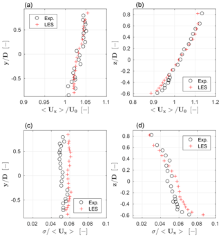
Figure 2 Normalized time-averaged streamwise velocity 〈u_x〉 (a, b) and turbulence intensity σ∕〈u_x〉 (c, d) 1.5 D downstream of the rotor. Left column: hub-height horizontal profile; right column: hub-centered vertical profile. Red + symbols: numerical results; black ∘ symbols: experimental measurements.

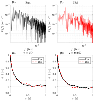
Figure 3 shows the experimental and simulated turbulent kinetic energy spectrum E(f) and autocorrelation r(τ) at hub height 1.5 D upstream of the rotor. The LES-computed spectrum appears to be in good agreement with the experimental one. The autocorrelation is computed as

$$\begin{array}{}\text{(4)}& r^j\left(\mathit{\tau }\right)=〈\left(u_x^j\left(t\right)-〈u_x^j〉\right)\left(u_x^j(t+\mathit{\tau })-〈u_x^j〉\right)〉,\end{array}$$

where $u_x^j$ is the streamwise component of the velocity at spatial point j. The integral timescale (O'Neill et al., 2004), defined as

$$\begin{array}{}\text{(5)}& T_{\mathit{\tau }}^j=\underset{\mathrm{0}}{\overset{\mathrm{\infty }}{\int }}{\displaystyle \frac{r^j\left(\mathit{\tau }\right)}{〈u_x^{j,\mathrm{2}}〉}}\mathrm{d}\mathit{\tau },\end{array}$$

is found to be 0.139 and 0.143 s for the experiment and simulation, respectively. These results indicate a good overall agreement between the simulation and experiment even at small scales, with a consequent correct estimation of flow mixture, wake recovery and other relevant features of the flow.

Figure 3 Turbulent kinetic energy spectrum E(f) at hub height 1.5 D upstream of the rotor for the experiment (a, black line) and simulation (b, red line). Autocorrelation r(τ) at hub height 1.5 D upstream of the rotor (c) and 0.25 D to its left, looking downstream (d).

3.2 Successor simulation

The computational setup for the wind turbine–wake simulation follows Wang et al. (2017a). The domain layout is shown in Fig. 1. The domain width is reduced to 3.9 D, which is 3.4 times less than the actual test section width to minimize the computational cost without affecting the results due to wall blockage. Note that the precursor width is about twice the width of the successor domain, simply because the same precursor is also used for nonaligned multi-turbine configurations (not discussed here) that, having a larger frontal area, require a larger inflow. The mesh uses three zones of increasing density. Zone 1 is the base mesh, with cubic cells 0.08 m in size, while zones 2 and 3 have cubic cells of 0.04 m and 0.01 m, respectively. Less than 1 % of the total mesh is composed of polyhedral cells, while all others are cubic.

Two different flow conditions are considered in the present study. In the first case, the flow velocity is obtained from a lidar-scanned low-turbulence (<2 %) inflow condition (van Dooren et al., 2017). Measurements also accounts for a slight nonuniformity of the flow within the wind tunnel (Wang et al., 2017a). In the second case, as previously explained, the output of the passively generated turbulent precursor simulation was instead used as an inlet for the successor simulation.

The treatment of the domain walls is as follows. Dirichlet-type nonslip wall conditions for $\stackrel{\mathrm{̃}}{\mathit{u}}$ are used for the tunnel ceiling and floor. Neumann-type conditions for pressure and temperature and mixed-type conditions for $\stackrel{\mathrm{̃}}{\mathit{u}}$ are used for the side walls, enforcing a null component of the velocity normal to the side surfaces to ensure mass conservation. The eddy viscosity μ_t is set with Neumann conditions on the left–right tunnel walls. For the ceiling and floor, μ_t is set with Dirichlet conditions to the fixed value $\mathrm{1}\times {\mathrm{10}}^{-\mathrm{5}}$ m² s⁻¹ in the low-turbulence case, while a wall model is used for the moderate-turbulence condition.

Dirichlet-type nonslip wall conditions are used for the IB-modeled nacelle and tower in the low-turbulence case, for which a laminar boundary layer (or, at least, a not fully developed turbulent boundary layer) is expected to extend over the entire IB surface due to the steadiness of the incoming flow. Despite the maximum y⁺ being equal to 50 on the IB surfaces, a wall function cannot be used here, as it could properly model only a fully developed turbulent boundary layer. Due to the coarse grid, an overestimation of the boundary layer thickness on the IB-modeled bodies is expected, which in turn will lead to an overestimation of the blockage induced by the turbine nacelle and tower.

Slip wall IB surface conditions are used for the moderate-turbulence case in order to mitigate numerical stability issues. Although this neglects the boundary-layer-induced blockage and turbulence, results indicate a negligible impact on the downstream wake profile. This is probably explained by the background turbulence that, by enhancing mixing, diffuses the signature of the tower and nacelle on the downstream flow.

4 Experimental setup

Tests were performed with the G1 scaled wind turbine model, whose rotor diameter and optimal TSR are equal to 1.1 m and 8.25, respectively. The model, already used within other research projects (Campagnolo et al., 2016a, b, c), is designed to have realistic wake characteristics, with shape, deficit and recovery that are in good accordance with those of full-scale machines. The model features active individual pitch, torque and yaw control that, together with a comprehensive onboard sensorization (including measures of shaft and tower loads), enables the testing of turbine and farm-level control strategies.

The flow within the wind tunnel was measured with hot-wire probes or stereo PIV. The latter technique was used to measure the flow characteristics in the near-wake (0.56 D) and far-wake (6 D) regions. The measurement planes cover a significant fraction of the wind turbine wake. In order to achieve a higher spatial resolution of the velocity field, the measurement area was divided into several windows with small overlaps between them. A rapid scanning of the entire measurement area was achieved by the use of an automated traversing system moving both the laser and the cameras. The measuring windows were divided into 32×32 pixel interpolation areas, which resulted in an approximate spatial resolution of 15 mm. For each measuring window, 200 pairs of images were acquired (per camera) without phase lock, resulting in time-averaged flow field measurements. Additional details concerning the PIV instrumentation are given in Campanardi et al. (2017).

5 Result and analysis

5.1 Baseline simulation and parameter tuning

The baseline simulation represents an isolated flow-aligned wind turbine. The machine is operated in a low-turbulence flow with a rotor-averaged inflow velocity equal to 5.9 m s⁻¹, which is slightly lower than the G1 rated speed (6.0 m s⁻¹).

This first case is used to determine the optimal values of the Smagorinsky constant C_s and the gamma scheme parameter β_m. The same tuned parameters are used for all other simulations in the rest of this work. This first test case is also used to verify the effects of the Gaussian width ϵ, which is used to project aerodynamic forces from the lifting lines onto the computational grid. In fact, it was observed that this projection may have a significant effect on the results, including rotor power and thrust. In principle, ϵ should be set to 2–3 times the cell size, i.e., $\mathrm{2}h\le \mathit{ϵ}\le \mathrm{3}h$ (Martinez et al., 2012). It was found that the dependency of the rotor aerodynamic power on ϵ is significantly reduced if the integral velocity sampling approach is used (Churchfield et al., 2017). For instance, if ϵ increases by 30 %, power will increase by 13 % if the traditional point-wise velocity sampling approach is used, but only by 5 % when using the integral velocity sampling method. In fact, in the point-wise approach a variation of ϵ reshapes the Gaussian curve, in turn changing the peak value and eventually affecting the calculated aerodynamic power, while the integral approach uses a weighted average that mitigates the reshaping effect (Churchfield et al., 2017).

Using a simple trial-and-error approach, the three parameters ϵ, C_s and β_m (in the near wake) were set to 0.025, 0.13 and 0.45, respectively. Given the low turbulence of the present case, the experimentally measured rotor speed was very nearly constant, and its average value was used in the simulation.

The rotor integral quantities of power and thrust are compared first by time averaging over 10 s. The wind turbine power was found to be equal to 45.79 W in the experiment and equal to 45.45 W for LES, showing a good agreement between these two values. A slightly larger discrepancy was obtained for the thrust, which was found to be 15.18 and 16.05 N for the experiment and simulation, respectively. This may be explained by the fact that thrust is directly measured at the shaft in the numerical simulation, while it is reconstructed from the fore–aft bending moment at the tower base in the experiment. This requires estimating the contribution of the nacelle and tower, which is done by a dedicated experiment performed on the wind turbine without the blades. As a result, this indirect calculation of the experimental thrust is affected by approximations, and it cannot be regarded to be as accurate as the measurement of rotor torque (and hence of power).

Next, the characteristics of the wake are compared between PIV measurements and the CS LES simulation. Figure 4 shows streamwise velocity contours on a plane 0.56 D downstream of the rotor. Measurements are missing from two areas left and right of the rotor disk; due to the close proximity of the measuring plane with the wind turbine, part of the nacelle (which is white) was in the background, leading to a wrong correlation between the PIV images. Apart from the two missing spots, the LES contours are similar to the PIV ones both in terms of wake width and deficit. The wake deficit for LES is on average 1.3 % higher than the experiment.

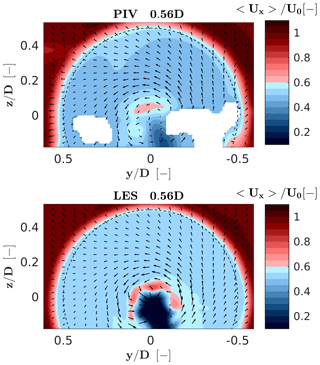
Figure 4 Streamwise velocity contours for the CS LES model and PIV experimental measurements, on a plane 0.56 D downstream of the rotor. Black arrows indicate the crosswind velocity component at a number of sampling points.

The figure also shows that the simulation overestimates the local wake deficit behind the nacelle and tower as a result of the enhanced blockage effect mentioned in Sect. 3.2. Indeed, the current mesh resolution (high y⁺) implies a thicker boundary layer, which in turn produces a higher blockage with a consequent larger flow separation, tower shedding and induced turbulence. This problem could be mitigated by a suitable refinement of the mesh near the IB, which would come at the price of a significant increase in the computational cost.

Next, hot-wire probe measurements are used to compare wake profiles at 3, 4, 7 and 8 D downstream positions. Figure 5 shows horizontal (top row) and vertical (central row) profiles of the normalized time-averaged velocity, as well as horizontal profiles of turbulence intensity (bottom row). The plots report results for the CS model, the LDS model and experimental measurements. The CS case includes two sets of results, one obtained including the effects of the nacelle and tower in the model and one obtained neglecting these two components. Comparing these two curves with the experimental results clearly indicates that the near-wake profile is more accurately represented when the nacelle and tower are included in the model, as already noted by other authors (Santoni et al., 2017). This may be particularly true for the present scaled wind turbine, for which these two components are relatively bigger than in full-scale machines. Indeed, the sum of the frontal area of the nacelle and the portion of the tower located within the rotor swept area A is 0.037 A, while it is 0.023 A for the NREL 5 MW wind turbine (Jonkman et al., 2009). Although this parameter is larger for the G1, it is expected that the effects of the nacelle and tower on wake evolution might not be negligible even for typical multi-MW wind turbines (Wang et al., 2017b). All other simulations reported in this work were performed including the nacelle and tower in the model.

Both CS and LDS show a good agreement with the experimental curves. Indeed, the temporally and spatially averaged streamwise velocity difference $〈\mathrm{\Delta }{u}_x〉=\left(〈u_{x,\text{LDS}}〉-〈u_{x,\text{CS}}〉\right)/〈u_{x,\text{CS}}〉$ between the CS and LDS models is consistently less than 1 % at all downstream distances. Results indicate that the LDS model does not provide significantly more accurate results than CS, while at the same time it requires a 20 % larger computational effort caused by the solution of its two extra transport equations. Moreover, turbulence intensity plots seem to indicate a slightly better match of CS to the experiments than LDS. Based on these results, all other simulations in the present paper were based on the CS model.

The rotor-averaged streamwise velocity difference between the simulation (with nacelle and tower) and experiment $〈\mathrm{\Delta }{u}_x〉=\left(〈u_{x,\text{sim}}〉-〈u_{x,\text{exp}}〉\right)/〈u_{x,\text{exp}}〉$ is equal to −2.7 %, −1.6 % and −1.3 % at 3, 4 and 8 D, respectively. The root mean square (RMS) error can be used to quantify the spatial fit between simulations and experiments, and it is defined as

$$\begin{array}{}\text{(6)}& \text{RMS}(\cdot )=\sqrt{{\displaystyle \frac{\mathrm{1}}{N}}\sum _{j=\mathrm{1}}^N{\left(〈(\cdot {)}_{\text{sim}}^j〉-〈(\cdot {)}_{\text{exp}}^j〉\right)}^{\mathrm{2}}},\end{array}$$

where 〈(⋅)^j〉 is a generic time-averaged quantity at a given spatial point j. At the various downstream distances, RMS(u_x) equals 0.34, 0.33 and 0.15 m s⁻¹, respectively. As expected, the matching of simulations with experimental measurements improves when moving downstream. Indeed, if rotor thrust is well predicted, flow mixture is properly resolved and numerical diffusion is suitably controlled, then the simulation results in a fully developed wake that correlates well with the experiment. The far-wake profile can be approximated by the single Gaussian distribution used in some engineering wake models (Larsen et al., 2007; Renkema, 2007).

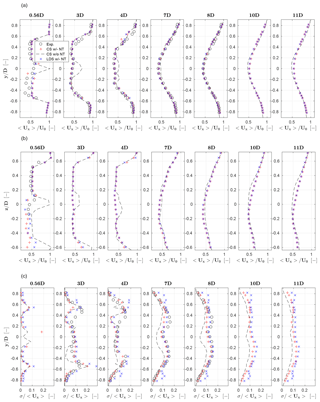
Figure 5 Profiles of normalized time-averaged streamwise velocity 〈u_x〉∕U₀ along hub-height horizontal lines (a) and along vertical lines through the hub (b). Turbulence intensity σ∕〈u_x〉 along hub-height horizontal lines (c). Red + symbols: CS model with nacelle and tower; black dashed line: CS model without nacelle and tower; blue × symbols: LDS model with nacelle and tower; black ∘ symbols: experimental results.

LES underestimates the rotor-averaged turbulence intensity σ∕〈u_x〉 by 23 %, 12 % and 12 % at 3, 4 and 8 D, respectively, while the rotor-averaged root mean square error RMS(σ∕〈u_x〉) is 0.04, 0.02 and 0.02 at these same positions. The turbulence intensity profiles in Fig. 5 clearly show that matching is not as good as in the case of the streamwise velocity, especially in the near-wake region where tip vortices are not resolved enough and tower shedding is overpredicted. Here again, the problem could be mitigated with a finer grid, which would lead to increased computational costs.

Comparing the turbulence intensity results with and without the nacelle and tower shows that there is an increased turbulence in the wake of the former case, which causes an earlier vortex breakdown and produces a higher turbulence intensity at the far wake. In turn, this generates a faster wake recovery, as shown in the speed deficit plots. Here again, this confirms the need for including the nacelle and tower in the simulation.

5.2 Low-turbulence inflow simulation

In this section, the characteristics of the LES framework are assessed with reference to three wake control strategies, namely power derating (or axial induction control), wake steering by yaw misalignment and wake-enhanced recovery by cyclic pitch control (CyPC). The flow conditions and setup of the simulations are the same as described earlier in the baseline case.

5.2.1 Power derating

Power derating was accomplished in the experiment by providing the turbine power controller with modified values of the rotor speed and torque. Specifically, for a power partialization factor p_f, the reference rotor speed is modified as $\sqrt[\mathrm{3}]{p_{\mathrm{f}}}\mathrm{\Omega }$, while the torque is modified as $\sqrt[\mathrm{3}]{p_{\mathrm{f}}^{\mathrm{2}}}Q$. This corresponds to having set the rated wind speed to the value $\sqrt[\mathrm{3}]{p_{\mathrm{f}}}{U}_{\mathrm{\infty }}$; since this is lower than the current wind speed U_∞, the machine is now effectively operating in the full power region. Therefore, the collective blade pitch controller automatically adjusts the pitch setting to track the new reference rotor speed.

The resulting pitch and rotor speed changes modify the angle of attack and Reynolds number at the blade sections. Therefore, tests that include power derating are useful for evaluating the quality of the identified multi-airfoil tables. Indeed, to accurately estimate rotor power and thrust, the lifting line airfoil polars need to match the aerodynamic characteristics of the corresponding blade sections in order to generate and project the proper body forces onto the fluid domain.

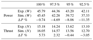
Simulations are conducted by prescribing the rotor speed and blade pitch measured in the experiment. Four power settings are considered, namely 100 %, 97.5 %, 95 % and 92.5 % of rated power. Figure 6 shows wake velocity profiles measured at hub height at a 4 D downstream position. For all cases, rotor-averaged speed error 〈Δu_x〉 and RMS(u_x) are about 1 % and 0.25 m s⁻¹, respectively. A quite satisfactory agreement between the simulation and experimental results can be noticed, although partialization seems to have only a modest effect on wake profile. Turbulence intensity profiles are not presented here, since the quality of the comparison is very similar to the one of the baseline case.

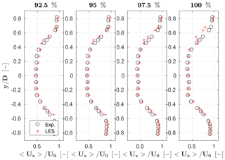
Figure 6 Normalized time-averaged streamwise velocity 〈u_x〉∕U₀ profiles at 100 % and 92.5 % power settings, measured at hub height and 4 D downstream of the rotor. Red + symbols: LES; black ∘ symbols: experimental results.

However, the situation is less satisfactory for rotor power and thrust, as shown in Table 2. Results indicate that power is particularly off, while thrust is affected by somewhat smaller errors. This might indicate a possible discrepancy in the behavior of the aerodynamic coefficients – especially of drag – with respect to the angle of attack. To verify that polars are indeed the culprit, several tests were conducted to check the effect of the Gaussian width ϵ. Indeed, one can tune ϵ to nearly exactly match the experimental results for each value of the curtailment factor. There is, however, not a single ϵ that is able to accommodate the investigated range of curtailments. On the other hand, keeping ϵ fixed, one can observe that the errors in power and thrust grow as the extent of power curtailment increases (and therefore as the angle of attack at the blade sections changes). These results seem to support the hypothesis that the slopes of the lift and drag coefficients with respect to the angle of attack are not calibrated well. To improve this aspect of the model, the polar calibration is being improved by a more sophisticated statistical weighting of the various experiments and by considering a span-wise variability of the Reynolds number.

Table 2 Power and thrust at 100 %, 97.5 %, 95 % and 92.5 % power settings.

5.2.2 Wake steering by yaw misalignment

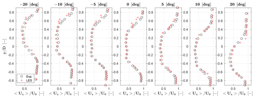
Next, the LES model is verified in yaw misalignment conditions, which are relevant to wake deflection control. Hub-height wake profiles measured in low-turbulence conditions are used for the comparison for yaw misalignment angles of ±5, ±10 and ±20^∘.

Simulated and measured longitudinal speed profiles are presented at a downstream distance of 4 D in Fig. 7. Similar results were obtained at other distances, but are not reported for space limitations. The maximum rotor-averaged difference 〈Δu_x〉 between the simulation and experiment is 4.1 % and corresponds to the 20^∘ case, while the maximum RMS(u_x) is 0.35 m s⁻¹ at −10^∘. The average 〈Δu_x〉 and RMS(u_x) over the six yaw cases are equal to 1.6 % and 0.29 m s⁻¹, respectively. The results indicate a good agreement between the simulation and measurement, both in terms of wake deficit and pattern. Note, however, that the 1.6 % average speed error would correspond to a 4.8 % power error for a second wind turbine operating in full-wake shading at this downstream difference, a value that is small but not completely negligible.

Figure 7 Normalized time-averaged streamwise velocity profiles at hub height for different yaw misalignments 4 D downstream of the rotor. Red + symbols: LES; black ∘ symbols: experimental results.

5.2.3 Enhanced wake recovery by cyclic pitch control

A third wake control strategy in the same low-turbulence conditions is considered, in which the rotor blades are cyclicly pitched. The effect of cyclic pitching is changing the angle of attack of the blade sections cyclically over one rotor revolution. In turn, this results in an azimuthal change in the out-of-plane forces generated by the section, which then has the effect of correspondingly modifying the local induced velocity. A simple analytical model of the effects of cyclic pitching was developed in Wang et al. (2016). The analysis showed that, as already noticed by other authors (Fleming et al., 2014), CyPC has some effect on the speed of recovery of the wake, but results only in a very modest deflection of its path. In fact, wake deflection by yawing is driven by the tilting of the rotor thrust, which results in a significant lateral force being applied onto the flow. On the other hand, CyPC does modify the induced velocity, but only generates negligible lateral forces. In addition, it was observed that CyPC also results in large moments being generated in the rotor fixed frame, which further questions the practical applicability of this wake manipulation strategy. Nonetheless, CyPC is considered here to further verify the characteristics of the LES framework in operating conditions that differ significantly from the ones in the previous test cases.

Each blade is pitched according to ${\mathit{\theta }}_i={\mathit{\theta }}_{\mathrm{0}}+{\mathit{\theta }}_{\mathrm{c}}\cos ({\mathit{\psi }}_i+\mathit{\gamma })$, where θ₀ is the collective pitch constant, θ_c the 1 P pitch amplitude, ψ_i the blade azimuth angle (clockwise looking downstream and null when the blade is pointing vertically up) and γ the phase angle (with the same origin and positive sense as ψ). The CyPC parameters were set as θ₀=0^∘, θ_c=5.3^∘ and γ=270^∘.

Given the effects of CyPC on the induced velocity and on the near-wake behavior, a more complete analysis can be performed by using the PIV measurements than considering the simple hub-height line scans obtained by hot-wire probes. Figure 8 reports, at left, the streamwise velocity just behind the rotor ($x/D=\mathrm{0.56}$), which is a distance for which few results have been previously reported. The images show that the use of CyPC has a strong effect on the wake structure, leading to a marked unsymmetrical shape. Indeed, the phase angle γ=270^∘ implies that blades have maximum pitch and hence produce the minimal rotor-plane-normal force in the left part of the rotor, as shown in the figure, which in turn exhibits the lowest induction and highest resulting longitudinal flow speed. A comparison between experimental and numerical results shows that there is, in general, a good qualitative agreement and that the main distortion effects caused by CyPC are reasonably captured. The rotor-averaged error 〈Δu_x〉 between the simulation and measurement is 2.69 %, while RMS(u_x) is 0.79 m s⁻¹.

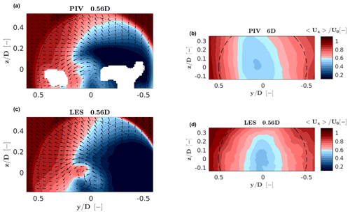
Figure 8 Streamwise velocity contour plots for the PIV measurements (a, b) and LES model (c, d) measured 0.56 D (a, c) and 6 D (b, d) downstream of the rotor. Black arrows indicate the crosswind velocity component at a number of sampling points.

The discrepancy between the simulation and experiment is 2 times larger than in the baseline case. One possible reason for this is that unsteady aerodynamic effects of the airfoils are neglected. This could be improved by using unsteady aerodynamic models in the lifting line, including, for example, a Theodorsen correction and a dynamic stall model. Although the Beddoes–Leishman approach (Moriarty and Hansen, 2005) is implemented in FAST and therefore could be readily used in the present LES framework, the model requires the definition of several airfoil-dependent parameters, which would need to be specifically calibrated for the low-Reynolds airfoils used on the G1 scaled wind turbine.

The comparison of LES and the experiment in the far wake (6 D) is slightly better, as can be observed in the right part of Fig. 8. The wake recovery is reasonably good in terms of flow speed, although the slight tilting towards the right shown by the PIV measurements is not apparent in the LES results. Lastly, it should be remarked that CyPC leads to a faster recovery of the wake than in the baseline case, as already noted by Wang et al. (2016). In principle, this could be of interest for wind farm control, although, as previously mentioned, the large resulting loads exerted on the rotor probably limit the practical applicability of this control concept.

5.3 Moderate-turbulence inflow simulation

Next, a turbulent case is considered in which a flow characterized by a 6 % hub-height turbulence intensity is generated by the precursor simulation described in Sect. 3.1. The wind turbine model is aligned with the streamwise flow direction and the hub-height wind speed is equal to 4.76 m s⁻¹ (partial load region). The simulated wind turbine operates in two different modes, namely with a fixed rotating speed of 720 RPM and blade pitch angle of 1.4^∘ (which are the values measured on the scaled model in the experiment) or with a controller in the loop (Bottasso et al., 2014).

The aerodynamic power output, averaged over a 60 s time window, is equal to 31.0 W for the experiment and to 30.5 and 31.2 W for the prescribed speed and closed-loop torque simulations, respectively. In this latter case, the average rotor speed was only 2.2 % higher than the one measured on the wind turbine, which clearly indicates a good overall match of the numerical model with the experiment. On the other hand, the power standard deviation was 0.2, 0.6 and 0.3 W, respectively, for the experiment, prescribed speed and closed-loop simulations. Clearly, prescribing a constant speed to the rotor in the numerical simulation induces significant torque oscillations because the rotor cannot adjust to the turbulent flow fluctuations. When loads are of interest, it is therefore essential to also use a closed-loop controller in the simulation. However, in this case the simulation might drift away from the operating condition realized in the experiment if the numerical model has a significant mismatch with respect to reality. Apparently, this is not the case here, and the numerical model seems to be well in line with the experimental one.

Figure 9 shows the normalized time-averaged velocity and turbulence intensity profiles for the LES model and experiment at distances of −1.5, 1.4, 1.7, 2, 3, 4, 6 and 9 D from the rotor. The position at −1.5 D is outside of the induction zone, and the flow can be regarded as the undisturbed free stream. The LES curves show, in general, a good agreement with the experimental ones. Only the case of the closed-loop regulation is reported here, as results are nearly identical to the prescribed speed case. The rotor-averaged simulation error 〈Δu_x〉 is less than 1 % on average across all distances. From the near-wake (1.4 D) to the far-wake (9D) regions, the root mean square error RMS(u_x) is gradually reduced from 0.2 to 0.1 m s⁻¹. The comparisons all indicate that the LES results are in good agreement with the experimental ones.

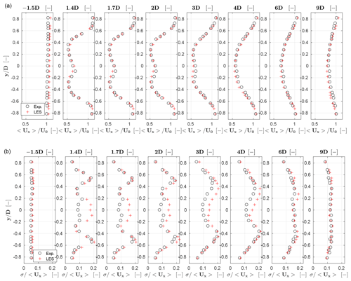
Figure 9 Normalized time-averaged streamwise velocity 〈u_x〉∕U₀ (a) and turbulence intensity σ∕〈u_x〉 (b) profiles at hub height. Red + symbols: LES; black ∘ symbols: experimental results.

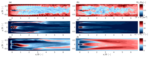
Contrary to the baseline low-turbulence simulation, the two turbulence intensity peaks induced by the blade tip vortices are well predicted in this case. To explain this phenomenon, we report in Fig. 10 for the low-turbulence (left) and moderate-turbulence (right) cases the instantaneous streamwise speed component u_x∕U₀, the vorticity 〈∇×u〉 and the turbulence intensity σ∕〈u_x〉 on a horizontal plane at hub height. As previously observed, the turbulent structures induced by the nacelle and tower are different for the two cases on account of the different boundary conditions on their surfaces.

Vorticity shed by the tips in the near wake is quite similar for the low- and moderate-turbulence cases. Turbulence intensity is, on the other hand, very different in the blade tip region for these two different ambient turbulence cases. In fact, the higher background turbulence of the turbulent inflow case triggers the instability of the tip vortical structures (Sørensen, 2011), which rapidly break down. The contour plots of the turbulent simulation clearly show that, starting from 0.1 D downstream, the tip vortices generate significant turbulence intensity, while vorticity quickly diminishes from 2 D downstream, signalling that the coherent tip vortices have broken down into smaller and less coherent structures. Quite differently, the low-turbulence case shows a persistent modest turbulence intensity and high vorticity up to about 4 D downstream of the rotor. In this case, capturing the right amount of speed fluctuations – which are mostly caused here by the tip vortices in contrast to the other case that is predominantly dominated by turbulent fluctuations – probably requires a denser grid than the one used here, and this explains the poor match with the experiments in this case in the near-wake tip region. Apparently, the same grid is, however, capable of representing the simpler turbulent case well. An analysis of tip vortex breakdown is reported in Troldborg et al. (2015) using a blade-conforming approach, which therefore uses significantly denser grids than in the present case.

Figure 10 Instantaneous streamwise speed component u_x∕U₀ (a, b), vorticity 〈∇×u〉 (c, d) and turbulence intensity σ∕〈u_x〉 (e, f). At left, low-turbulence case; at right: moderate-turbulence case.

6 Conclusions

This paper has employed an LES approach for the simulation of wind turbine wakes, obtaining a complete digital copy of scaled experiments performed in a boundary layer wind tunnel. The main goal of the paper was to try to quantify the ability of LES to represent operating conditions relevant to wind farm control. To this end, numerical results were compared to wind tunnel measurements of one single wind turbine, while multiple machines and wake interactions are studied in Wang et al. (2017b, 2018) and in other forthcoming papers. While this work does not have the ambition to develop a comprehensive validation activity, it represents a step in the direction of a better understanding of the capabilities and limits of the current high-fidelity simulation technology for wakes.

A low-turbulence normal-operation problem is considered first, showing that simulations are in good agreement with experiments both in terms of rotor quantities (thrust and power) and wake behavior. Next, the three wake control strategies of power derating, wake steering by yaw misalignment and wake-enhanced recovery by cyclic pitch control are studied. Results show a good agreement of simulations with experiments for yaw misalignment, but are less satisfactory for derating, probably on account of inaccuracies in the airfoil drag. The wake turbulence intensity shows some discrepancies, which were here attributed to a lack of refinement of the grid that in turn affects the breakdown of the near-wake vortical structures. Slightly less accurate results are obtained for cyclic pitching, possibly due to un-modeled unsteady airfoil aerodynamics.

The paper continues by considering a moderately turbulent wind. The characteristics of the simulated turbulent flow are in good agreement with measurements. The average streamwise velocity is within 1 % of the experiments, and the average turbulence intensity within 5 %–7 %, while the turbulent kinetic energy spectrum and integral timescale also exhibit a good matching. The wake characteristics are in very good agreement with the experiments, since tip vortices break down earlier than in the low-turbulence condition, relaxing the need for very dense grids in the near-wake region. The use of a controller in the loop leads to a more realistic response of the model turbine to the turbulent flow, which is important if the load response of the machine is of interest. Remarkably, the model in the loop also operates at essentially the same rotor speed as the experiment, which demonstrates the overall fidelity of the digital model to the experimental one.

Results shown in this work indicate that the present LES-ALM approach is a viable way of simulating scaled wind tunnel experiments. Results are, however, not perfect, and areas of improvement include a more sophisticated and accurate calibration of the airfoil polars, the inclusion of airfoil unsteady aerodynamic effects (which also call for the calibration of these models with dedicated data sets), and a more efficient refinement of the grid where necessary by the use of unstructured meshing and adaption techniques.

These encouraging results motivate and justify the application of the present simulation framework to the analysis of clusters of wake-interacting wind turbines, for which we have gathered an ample collection of data sets in multiple operating conditions. Hopefully, this will lead to a better understanding of wake behavior, which is of crucial importance for the design and operation of wind turbines and wind power plants. The final validation of the present and similar simulation approaches can undoubtedly benefit from the use of scaled wind tunnel experiments, as attempted in this work, as an intermediate step towards their application to the full-scale case.

Appendix A: Nomenclature

A	Rotor swept area
D	Rotor diameter
CD	Drag coefficient
CL	Lift coefficient
$C_k^{\mathrm{0}}$	Nominal coefficient
Cs	Smagorinsky constant
E(f)	Turbulent kinetic energy spectrum
J	Cost function
N	Number of available experimental observations
Q	Rotor torque
R	Covariance matrix
Tτ	Integral timescale
U∞	Free-stream wind speed
h	Grid size
pf	Power partialization factor
r(τ)	Autocorrelation
ui	Velocity component
y+	Dimensionless wall distance
α	Angle of attack
βm	Tunable constant for gamma scheme
γ	Phase angle
ϵ	Gaussian width
η	Span-wise location
θ	Blade pitch angle
ψ	Blade azimuthal angle
ρ	Density
σ∕〈ux〉	Turbulence intensity
τ	Time shift for autocorrelation analysis
Ω	Rotor speed
Δ⋅	Correction or difference
〈⋅〉	Averaged quantity
$\stackrel{\mathrm{̃}}{(\cdot )}$	Resolved quantity
ALM	Actuator line method
bi-CG	Biconjugate gradient
CFD	Computational fluid dynamics
CG	Conjugate gradient
CS	Constant Smagorinsky
CyPC	Cyclic pitch control
DIC-GS	Gauss–Seidel smoothing with diagonal incomplete Cholesky factorization
DILU	Diagonal incomplete LU factorization
GAMG	Geometric–algebraic multigrid
IB	Immersed boundary
LES	Large-eddy simulation
LDS	Lagrangian averaging dynamic Smagorinsky
Lidar	Light detection and ranging
NOC	Non-orthogonal corrector
PISO	Pressure-implicit with splitting of operators
PIV	Particle image velocimetry
RANS	Reynolds-averaged Navier–Stokes
Re	Reynolds number
RMS	Root mean square
TSR	Tip speed ratio