the Creative Commons Attribution 4.0 License.
the Creative Commons Attribution 4.0 License.
 | 31 May 2024
Dynamic analysis of the tensegrity structure of a rotary airborne wind energy machine
Gonzalo Sánchez-Arriaga
Álvaro Cerrillo-Vacas
Daniel Unterweger
Christof Beaupoil
The dynamic behavior of the tensegrity structure (helix) of a rotary airborne wind energy (RAWE) machine was investigated by combining experimental and numerical techniques. Taking advantage of the slenderness of the helix, a dynamic model for the evolution of its center line and the torsional deformation was developed by using Cosserat theory. The constitutive relations for the axial, bending, and torsional stiffness, which are a fundamental component of the model, were obtained experimentally by carrying out laboratory tests. Three scenarios of increasing complexity were then studied with the numerical tool. Firstly, a stationary solution of the model, i.e., with fixed ends and no rotation, was found numerically and used to verify the correct implementation of a numerical code based on finite elements. The stability analysis of this solution, which corresponds to the state of the structure just after deployment but before operation, showed that the natural periods of longitudinal, lateral, and torsional modes of the RAWE structure under consideration are around 0.03, 0.2, and 0.4 s, respectively. Secondly, the dynamics in nominal operation was investigated by keeping both end tips fixed and implementing a controller that adjusts the torque at the ground to reach a target angular velocity of 120 rpm. Key characteristic variables like the tension and the response times of the helix were obtained. Thirdly, the dynamics of the helix when the lower end is fixed and the upper end is driven in a circular motion of frequency f1 was studied experimentally and numerically. The tension of the helix in the experiment increased for f1 above a certain threshold, and the structure collapsed at f1≈5 Hz. Simulation analysis revealed a resonance of the structure at a higher frequency (around 13 Hz).
- Article
(2294 KB) - Full-text XML
- BibTeX
- EndNote


The increase in wind power density with altitude (Archer and Caldeira, 2009) constitutes an important driver for wind technologies. Conventional wind turbines have notably increased their size during the last few decades to reach higher winds. However, although control strategies have been developed to meet efficiency and reliability requirements (Njiri and Soffker, 2016), structural considerations may set an upper limit. Airborne wind energy systems (AWESs), mainly based on soft kites, rigid wings, or rotors linked to the ground by tethers, can harvest energy at high altitudes by using the tether tension or onboard wind turbines (Schmehl, 2018; Malz et al., 2022). In ground-gen AWE concepts the conversion from mechanical to electrical energy happens on the ground, whereas in fly-gen systems such conversion is done on the aircraft (Cherubini et al., 2015). Some of these technologies are in a precommercial state (European Commission, 2018; Blanch et al., 2022). Although it is still unclear which of them will dominate the market among the plethora of existing architectures (van de Kaa and Kamp, 2021), system reliability, operational robustness, and safety are crucially important aspects of system development (Salma et al., 2020) together with their performances in realistic vertical wind velocity profiles (Sommerfeld et al., 2019; Schelbergen et al., 2020; Sommerfeld et al., 2023).
An interesting subfamily of AWE systems involves concepts based on rotating kites or rotors that use the well-known phenomenon of auto-rotation for harvesting wind energy (Rimkus and Das, 2013). An example is a tethered autogyro system with four rotors in a quadrotor configuration that harvests energy and transmits it to the ground via the tether (Mackertich and Das, 2016). Rotating reel parotors, which combine rotary ring kites with ground-based rotating reel conversion systems (Benhaiem and Schmehl, 2018) and gyrocopter-type airborne wind turbines (Rancourt et al., 2016; Roberts et al., 2007), have been proposed. Prototypes of AWE systems aimed at the direct transmission of the mechanical torque produced by a set of kites or a flying rotor to a generator on the ground have also been manufactured and tested. The Daisy stack by Windswept and Interesting Ltd (Read, 2018) and the rotary AWE (RAWE) machine of SomeAwe (Beaupoil, 2017) belong to this category. These two concepts have in common the use of a light tensegrity structure (Motro, 2003) to transmit the torque to the generator and an auxiliary kite to provide extra lift and fix the elevation angle of the machine.
Flight testing activities with the RAWE machine showed that the tensegrity structure exhibits a rich dynamics that involves longitudinal, lateral, and torsional waves. The tensegrity structure has a helix-like shape that acquires a high torsional and bending stiffness when a traction load is applied. Finding the operational limits of the helix is crucial for the reliability of the RAWE machine. According to experimental tests, the structure can collapse if the torque is above a certain threshold (Beaupoil, 2022). For this reason, characterizing the axial, bending, and torsional stiffness of the helix, as well as having access to numerical tools capturing longitudinal, lateral, and torsional dynamics, is important. Numerical simulations can help to predict the operational boundaries and avoid hardware failure. Nevertheless, the modeling of the structure represents an important challenge that should balance fidelity and computational cost. Two dynamic models of different complexity have been developed in a previous study for the tensegrity structure of the Daisy stack (Tulloch et al., 2020, 2023): a simple spring-disk model and a multi-spring/multi-punctual mass model. The latter involves a higher number of degrees of freedom and can capture the variation in axial tension along the length of the structure. Interestingly, two stable-equilibrium states were predicted by the numerical simulations when the rotor dynamics was coupled with the spring-disk model (Tulloch et al., 2020). A steady-state model that uses aerodynamics and structural modules to analyze the performance of RAWE machines has been proposed (Wacker et al., 2023). The control problem was also studied by using a model with a small number of degrees of freedom (De Schutter et al., 2018), and the aerodynamics of the rotor was studied with blade-element theory and vortex computations (Pfister and Blondel, 2020). To the best of our knowledge there is a lack of knowledge about the axial, bending, and torsional stiffness of existing RAWE machines.
An important property of the tensegrity structures of RAWE machines is that they are slender; i.e., their unstretched length (L0) and characteristic radius (Rs) satisfy L0≫Rs. This work exploits this key feature to model the structure by using Cosserat theory that, due to its versatility, has been used in a very broad range of applications (Ramézani et al., 2011; Riahi and Curran, 2009). In this case, we use Cosserat rod theory to find a set of partial differential equations that govern the dynamics of the central line and its torsional deformation (see Sect. 2). This set of equations is appropriate for investigating in detail the rich dynamics observed in RAWE experiments because it captures the stretching, bending, and twisting of the structure. A finite-element method is proposed in Sect. 3 to approximate the partial differential equations by a set of ordinary differential equations. The axial, bending, and torsional stiffness, which naturally appear in the dynamic equations, have been determined experimentally in Sect. 4 for the RAWE machine of SomeAwe. Three scenarios of increasing complexity are studied numerically and experimentally in Sect. 5. Section 6 summarizes the conclusions. The code presented in this work is part of the open-source software LAKSA (Sánchez-Arriaga et al., 2017, 2019).
2.1 Kinematics considerations
Figure 1 shows a RAWE machine made of a tensegrity structure (helix) of unstretched length L0 that transmits the torque generated by a set of blades to a generator on the ground. The slenderness of the tensegrity structure, i.e., with its length being much larger than the characteristic length of its cross section, suggests using some approximations that help to simplify the mathematical analysis. In particular, we use Cosserat theory and only compute the evolution of the position vector of the central line of the helix and an additional angle that orients the cross section, which is assumed to be unshearable. These two variables are called r(s,t) and α(s,t), where and t are the unstretched arc length and time, respectively. Taking the helix as a one-dimensional Cosserat rod with an unshearable cross section has the advantage of extraordinarily simplifying the model while allowing us to capture the axial deformation, the bending of the helix, and the twisting of the helix. An inertial frame of reference 𝒮E with its origin at the generator, plane xE−yE spanning the ground, and the zE axis pointing downwards are introduced. We call iE, jE, and kE to the unit vectors along the three axes of frame 𝒮E. Therefore, is the origin of 𝒮E, and is the position vector of the hub of the blades (point T in Fig. 1). In this work, we use bold-italic characters to denote vectors, and bold-roman characters to denote matrices.
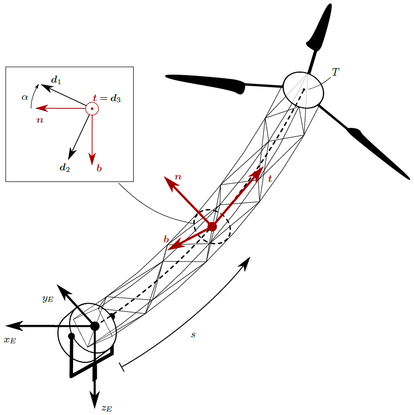
Following Buckham (2003), we define at every point of the center line a Frenet frame (𝒮F) with axes spanned by the unit vectors (). For small axial deformations of the helix
the vectors of the Frenet basis read
Although the same character is used in this work, the tangent vector t should not be confused with time t, which is a scalar and always written with a plain letter. The curvature and torsion of the center line are given by
where we denoted by the superscript ′ the derivative with respect to the unstretched arc length s. The derivatives of this basis with respect to the arc length are
where is the Darboux vector.
At every point of the center line we also define a local frame 𝒮D with director vectors and origin at the particular point of the center line. The director vector d3 points along the tangent vector t. Vectors d1 and d2 span the cross section of the helix and are directed along its principal axes of inertia. The director basis is related to the Frenet frame by a rotation of an angle α about the tangent vector t
The derivative of the director basis along the center line is
where
is the twist vector, and it involves the curvature κ and torsion γ of the center line. The scalar
is the total twist of the principal axes of inertia of the helix about the tangent vector t. The time evolution of the director vectors is given by an equation analogous to Eq. (6):
where the dot denotes the time derivative, and ωDEis the angular velocity of the local frame (𝒮D) with respect to the inertial frame (𝒮E). Vectors ωDE and K are linked by the constraint
which is found by differentiating Eq. (6) with respect to time and Eq. (9) with respect to the arc length. The angular velocities of frames 𝒮D and 𝒮F with respect to 𝒮E are related by .
2.2 Dynamic model
Momentum and angular momentum equations of the structure with total mass M read (see for instance Villaggio, 2005)
where FA is the aerodynamic force per unit length, and f and m are the internal force and torque, respectively. We also introduced the density and the two principal moments of the cross section of area A:
Regarding FA, we only consider the aerodynamic drag and write
where CD and ρ0 are the drag coefficient and the air density. We also defined the aerodynamic velocity (); ; the wind velocity (vw); and the characteristic transversal length (la), which can be approximated by the sum of the diameters of the bars of the helix. In our analysis we consider a constant wind velocity vector .
The model is completed by the constituent relations that depend on the elastic properties of the material and on the shape and the dimension of the cross section of the structure. Writing the twist vector as , the internal moment is (Love, 1944)
where E is Young's modulus, G is the rigidity modulus, and J is the torsion constant. Hereafter, we model the structure as a hollow cylinder of radius Rs and thickness hs. Therefore, we have from Eq. (13)
and, using Eq. (7), Eq. (15) becomes
The set of equations is simplified if some considerations based on the geometry of the structure and the forces and torques that are expected to act on it are taken into account. We start by assuming that and writing . The left-hand side of Eq. (12) then becomes
where we used Eq. (9). Regarding the right-hand side, we use Eq. (4) and write with to find
Equation (12) then becomes
The components normal to t of Eq. (20) give f⟂, and the total internal force then becomes
where we used Eq. (2). For the tension we assume Hooke's law:
This law is consistent with our assumption , which was also used in Eq. (2). For large deformations, the model should be revisited.
After substituting these results in Eqs. (11) and (20), one finds
The above set of equations describes the dynamics of the center line of the helix and its torsional deformation. Given appropriate initial and boundary conditions, they can be integrated numerically to find their evolution.
For convenience, we introduce the normalized variables
parameters
and normalized forces
We also changed the notation, and the primes now denote the derivative with respect to the normalized arc length . The equations of motion become.
with
and
Regarding the boundary conditions, we do not impose the exact conditions of a real rotary machine, i.e., coupling the dynamics of the structure and the rotor. Such a complete analysis is beyond the scope of this work that is focused on the helix. We assume that the position vector of the central line at coincides with the origin of the inertial system 𝒮E. At , we also impose a prescribed position. We then have
Additionally, we impose zero curvature at both tips,
and known torsional torques at and :
where M0(t) and MN(t) are the external torques imposed at the ends of the structure. Equations (38)–(39) involve the use of Eq. (3) and Eq. (37) in Eq. (8). As explained below, the initial conditions depend on the type of analysis.
Since our work does not couple the helix with a rotor, the torque at is a given function . Regarding the torque at , we implement the controller
where k1 and k2 are constant, and is given by the first equation in Eq. (56). Such a proportional-derivative controller adjusts the torque exerted at the ground to reach a (constant) target angular velocity at the first node.
Equations (30)–(31) were solved numerically by using a finite-element method. We introduce N elements and N+1 nodes, and with , and . For each element between nodes and , the variables and are written as (Buckham, 2003)
with . The shape functions are the twisted-spline polynomials:
where
is the local coordinate. One readily verifies that the coefficients and in Eqs. (41) and (42) coincide with the displacements and the rotation angles at the nodes and and with their second derivatives. This choice for the shape function thus gives continuity for , , , and . As explained in Appendix A, by assuming that the first derivative is continuous across the elements, we find relations between and and between and . Equations (41)–(42) for all the elements, together with relation Eqs. (A1)–(A4) and the boundary condition Eqs. (35)–(36), allow us to write the variables as
where ϕi and φi are 𝒞2 continuous functions, and the function just involves the boundary conditions (m0 and mN) and the shape functions. One readily checks that ϕi(0)=0 for i=1…N, ϕN(1)=1, and ϕi(1)=0 for .
Following a Galerkin method, we write Eqs. (30)–(31) in the weak form. We multiply Eq. (30) by ϕi with and Eq. (31) by φi with i=0…N and integrate between and to find
where we introduce the matrices and the vectors
Integrations by parts of Eqs. (48) and (49) yield
where we use for , Eq. (37), and define
Since i runs from 1 to N−1 in Eq. (55) and from 0 to N in Eq. (56), there are a total of equations for the 4N−2 unknowns, which are with and with j=0…N.
After constructing the vector
and the state vector
we find the following set of first-order ordinary differential equations:
The explicit form of matrix and the vector field g can be found from Eqs. (55), (56), and (40).
Several tests were carried out to verify the correct implementation of Eq. (61). For instance, to test the correct implementation of functions ϕj and φj and matrices Br, Cr, etc., some analytical functions satisfying the boundary conditions were proposed for and . The derivatives , , , , and were computed analytically and also by using the finite-element approach. It was verified that both results converge as the number of elements increases. The analysis of Sect. 5.1, where a stationary solution is found with an alternative numerical method, constitutes another test of the correct implementation of the finite-element method.
Three laboratory tests were carried out to find the values of EA, EI, and GJ for the tensegrity structure of SomeAWE Labs. Detailed information, drawings, and videos are in Beaupoil (2024). As shown in the three panels of Fig. 2, a segment of the helix with length equal to L0=6.76 m was clamped on a wall. As explained below, different types of loads were applied to determine the axial, bending, and torsional stiffness. For all the tests, a tension force Te was applied to the structure, and its values were taken of the order of around 200 N, which is the nominal tension during the regular operation of the RAWE machine. In cases (a) and (c) in Fig. 2, i.e., the axial and torsion tests, such axial force was applied by using a tension belt. In the bending experiment (case b), where there is a lateral displacement, a pulley and a ballast mass were used, and the position of the pulley was adjusted to apply the force normal to the displacement. Figure 2d displays the helix configuration during the axial test and the tension belt.
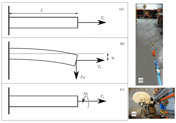
Figure 2Panels (a–c) show the sketches of the axial, bending, and torsion tests. Panels (d) and (e) display the helix in the axial test and the motorized eccentric arm explained in Sect. 5.3.
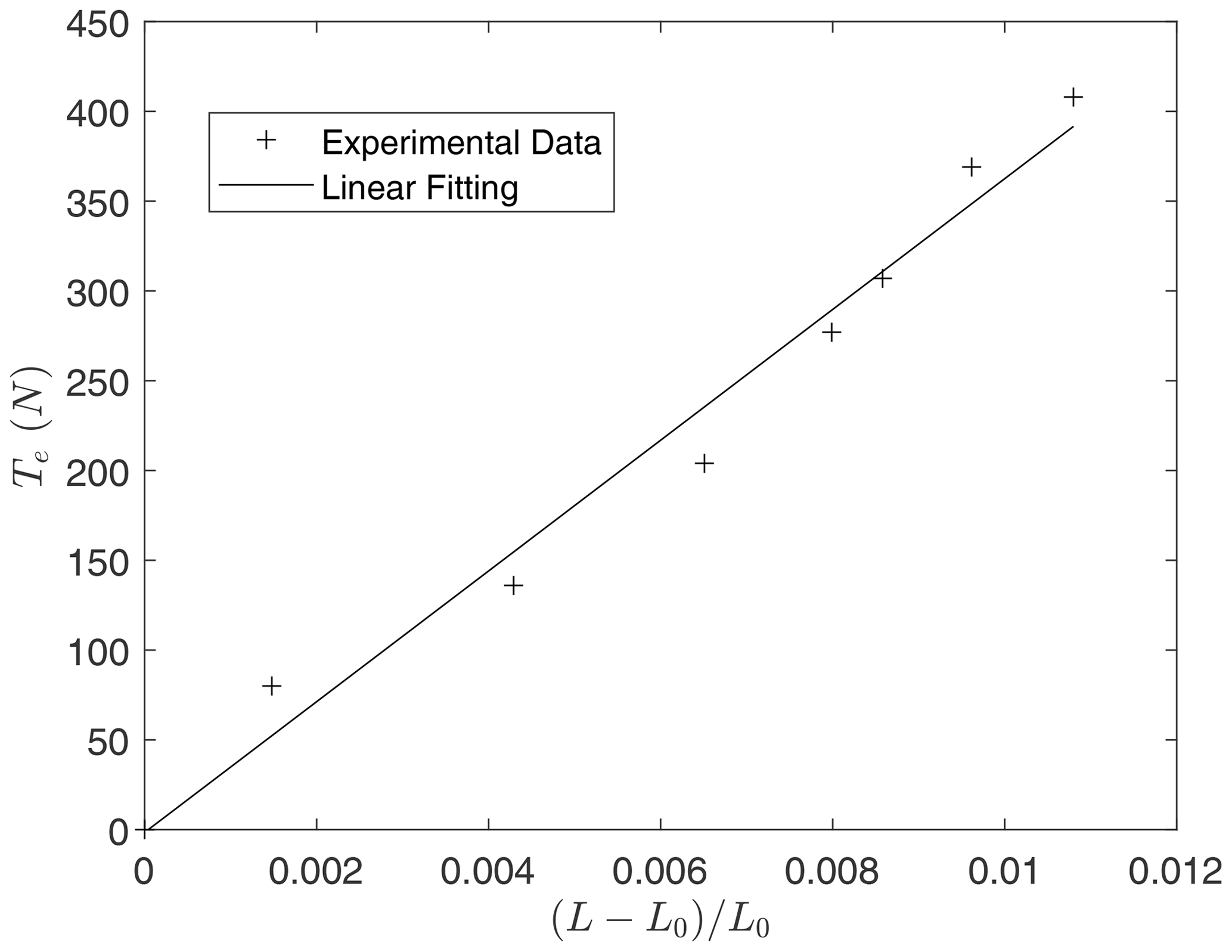
As shown in the top panel of Fig. 2, the EA product was found by applying an axial force Te and measuring the resulting length of the structure L. The axial force was varied by just increasing the mass of the ballast. For a linear material, the relation between the axial force and the length of the structure is
As expected, the experimental values of the strain are proportional to the applied force (see Fig. 3). The slope obtained with a linear regression is .
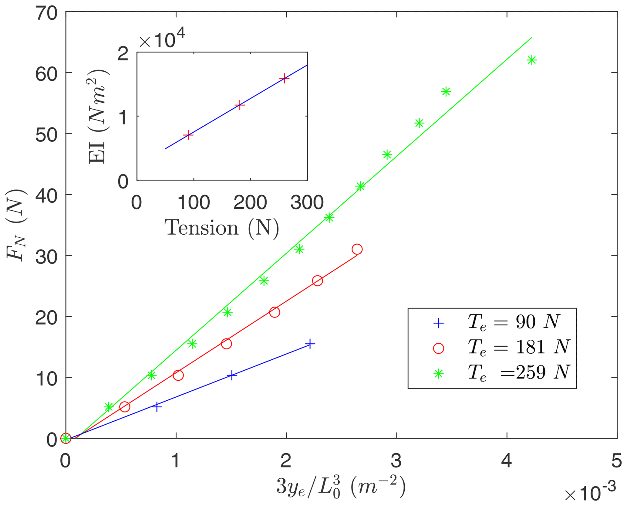
A classical bending test was carried out to determine the EI product of the helix. As shown in the middle panel of Fig. 2, a normal force of value FN was applied at the free end of the structure, and the vertical displacement ye was measured. Since the theoretical relation between both magnitudes is
measuring the pairs (FN,ye) and making a linear regression to the experimental data give the EI product. However, the bending stiffness of the tensegrity structure depends on the internal tension force. For this reason, the experiment was carried out for three different ballast masses, which yielded the tension forces Te= 90, 181, and 259 N. As shown in Fig. 4, for each value of the tension, the helix has a different bending stiffness (slope of the linear regression in the FN versus plane). The inset in Fig. 4 shows that the relation between the EI product and the tension is also linear and follows the law
As expected, the higher the tension, the higher the bending stiffness of the tensegrity structure.
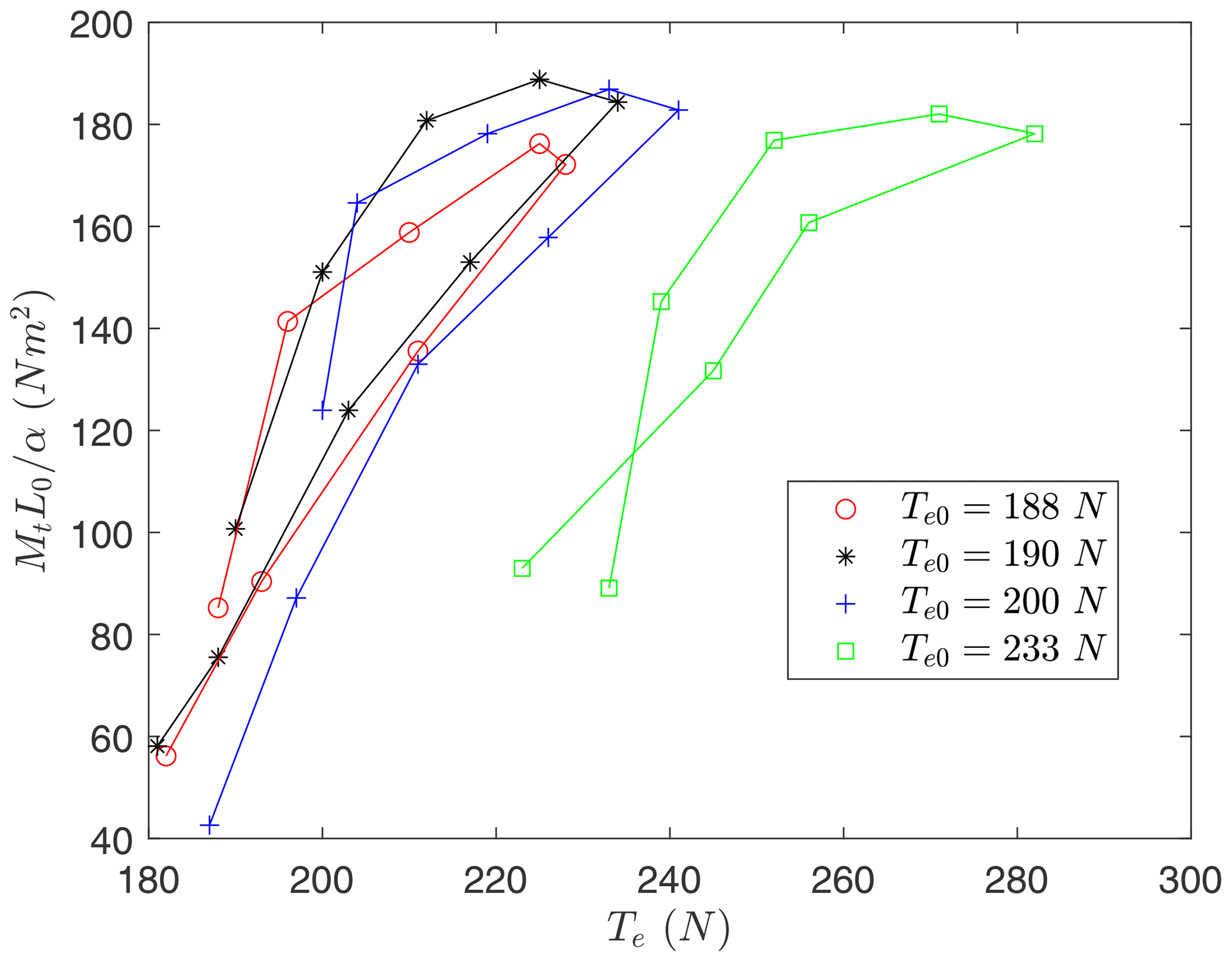
Difficulties were found for the experimental determination of the torsional stiffness. As shown in the bottom panel of Fig. 2, the helical structure was tightened with the ballast mass to induce a tension force Te0 for zero torsion angle (α=0). A torsion torque Mt was then applied at the free end of the structure until the torsion angle took a certain value α. The tension force Te was then measured with the hanging scale, and it was found that it was higher, Te>Te0. Measurements of Mt, α, and Te were taken by first increasing Mt sequentially and with an increment of the torsion angle of around Δα=10°. After reaching a maximum torsion angle of about 50°, Mt was lowered to produce decrements in the torsion angle of until α=0 was reached. Four complete cycles raising and lowering the torsional torque were completed, and measurements for the three variables (Mt, α, and Te) were taken. The maximum value of Mt in the experiment was around 25 N m, which is consistent with the torque measured during the real operation of the RAWE machine.
In principle, a simple model for the relation between the torsion torque and angle is
However, the experiment revealed that the behavior of the helix is not so simple. As seen in Fig. 5, the ratio , which may coincide with GJ according to Eq. (65), versus the tension force Te present hysteresis. For the three tests covering a tension range between 180 and 240 N, the repeatability of the measurements is satisfactory, but it is clear that the ratio cannot be parametrized by the tension force Te alone. In a fourth test, the torsional behavior of the structure was explored at an even larger tension value, and the amplitude of the hysteresis cycle was similar. These results indicate that the value of the torsional rigidity depends not only on the instantaneous value of the torsion angle and internal tension but also on the history of the helix. Such a feature may be due to the peculiar construction of the tensegrity helix, which involves bars under compression, tethers, and knots. The unavoidable friction in the experimental setup may also play a role. For this reason, we decided in later analysis to set a nominal value for GJ of 140 N m2, which is consistent with the experimental results of Fig. 5 for Te=200 N.
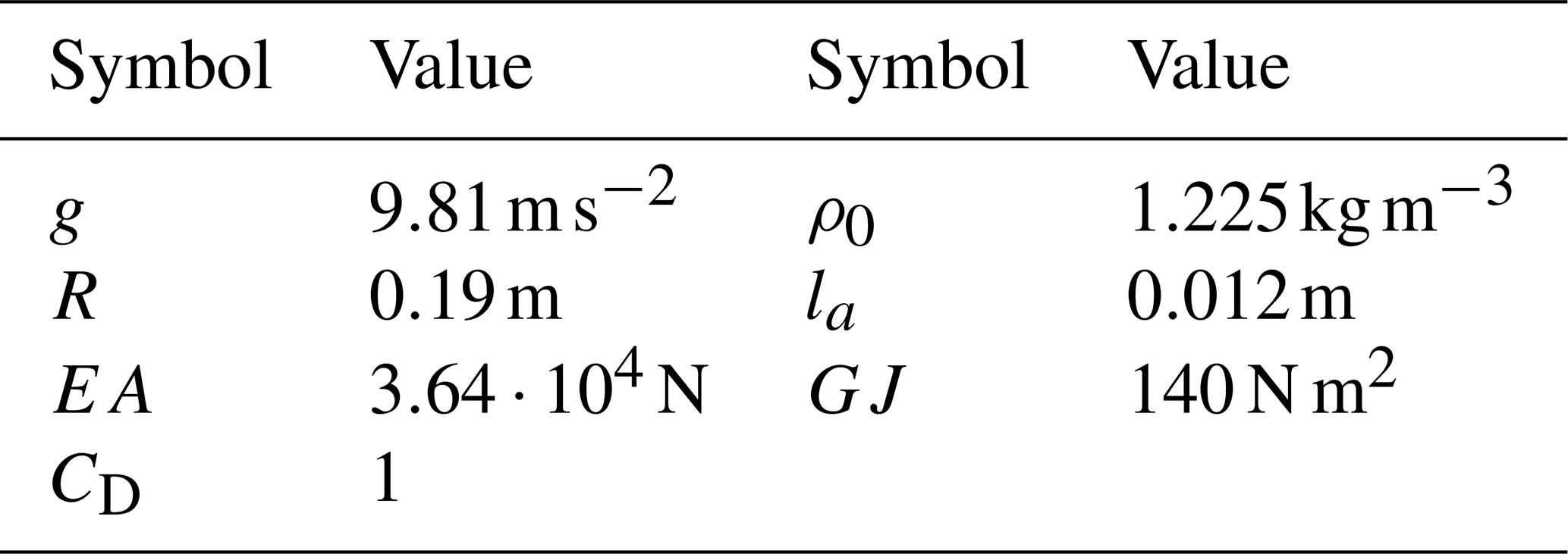
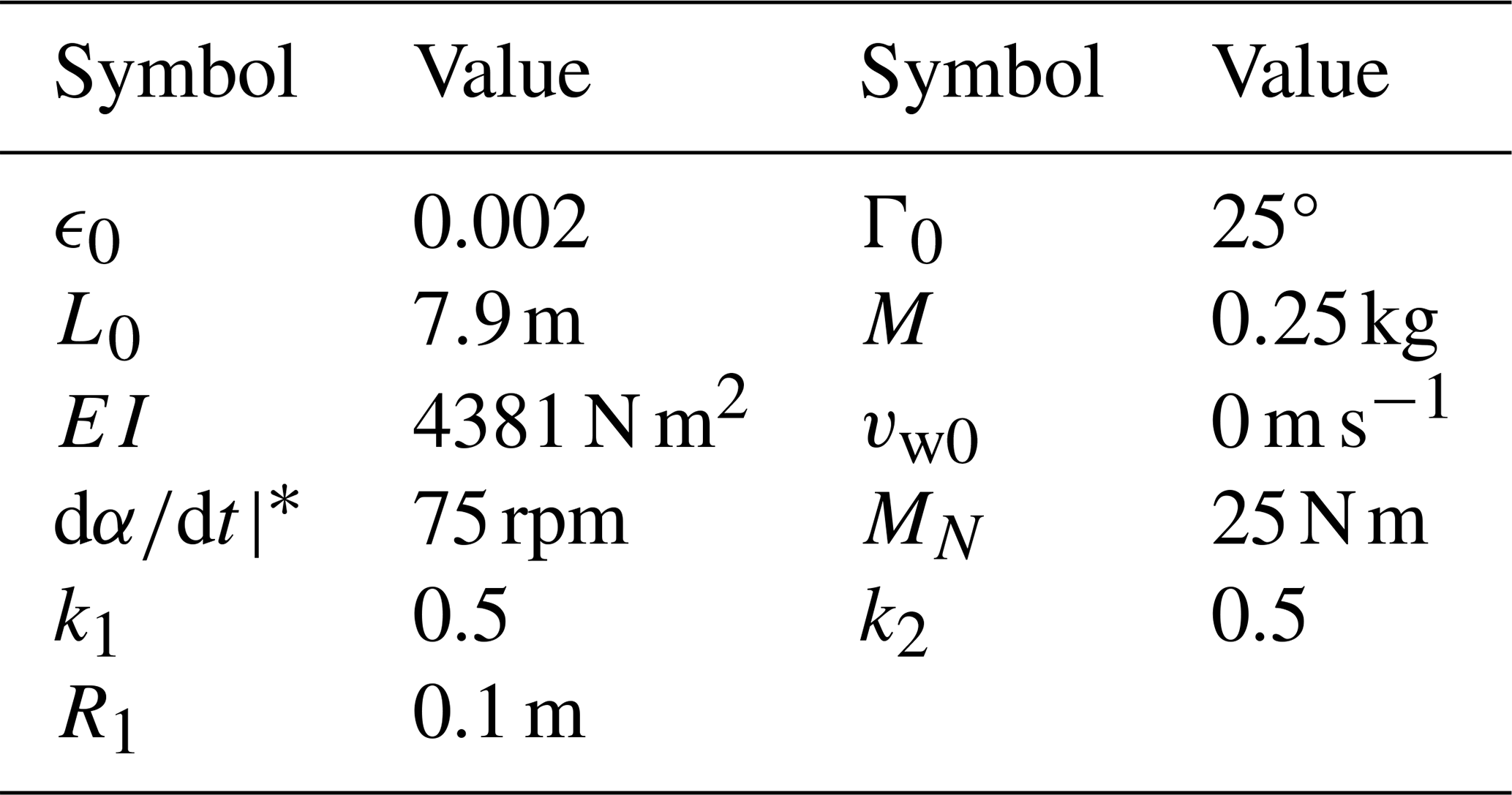
This section studies three different dynamic scenarios of the helix. For all of them we used the parameters shown in Table 1.
5.1 Stationary solutions with fixed ends
We consider a helix with the properties of Tables 1 and 2, which correspond to the characteristics of the structure of the RAWE machine of SomeAwe. Since its nominal tension during regular operation is around 200 N, we set the elongation of the initial condition as and compute EI by using Eq. (64) with Te=200 N.
Table 2Parameters used in the analysis of solutions with fixed ends.
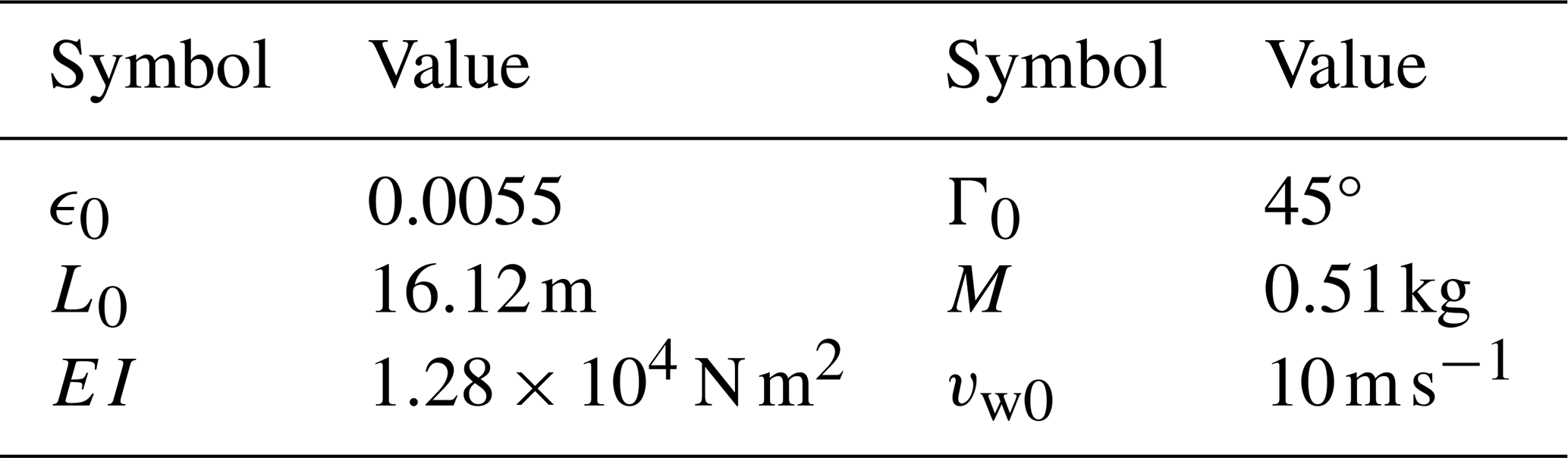
The analysis focuses on stationary solutions of Eq. (61); i.e., all the variables are time independent, and the time derivatives of and vanish. The boundary conditions are given by Eqs. (35)–(36), and
where Γ0 is the elevation angle of the helix, ϵ0 is a parameter that determines its elongation, and iE and kE are unit vectors of frame 𝒮E. We restrict the analysis to solutions of the type and with . Since the proposed solution is contained in the xE−zE plane and no torque is applied at the ends of the helix, the torsion vanishes (), and Eq. (31) is automatically fulfilled. Regarding Eq. (30), and after using (), it becomes the following set of ordinary differential equations:
with , , and
The solution of System (67) compatible with the boundary conditions (35)–(36) was found by using a shooting method. The equations were integrated numerically with a Runge–Kutta method, and the state at s=0 was given by . Constants and zsss0 were varied with a shooting method until the conditions , , and were satisfied. Once the solution was found, we constructed from it the state vector xs of Eq. (60). Its substitution on the right-hand side of Eq. (61) revealed that it is indeed a stationary solution because we found . The larger the number of finite elements, the lower the value of . This result constitutes an important test about the correct implementation of the finite-element method because xs was found with an alternative numerical algorithm (an integration of the equations with a Runge–Kutta method).
The linear stability of the stationary solution was then investigated in the framework of Eq. (61) and setting N=2. Using the vector xs obtained with the shooting algorithm as an initial guess, we found the state vector satisfying the condition in Eq. (61) with a Newton–Raphson method. Afterwards, the Jacobian matrix of flow f at and its eigenvalues were computed. As shown in Table 3, the stationary solution is stable because the eigenvalues are pure imaginary numbers or complex numbers with a negative real part. There are two longitudinal modes where the dominant components of the eigenvectors are and . The first of them has a short period (fast mode), which can be approximated by that is valid for thin and elastic rods of Young's modulus E and density ρ. In our case it reads s and matches with the first mode in Table 3. There is also a lateral mode dominated by displacements contained in the xE−zE plane. The period of this mode is well described by the one of a string of linear density ρL, length L0, tension T, and fixed tips. The nth harmonic vibration has wavelength and velocity . The period for n=2 in our case reads s, where the tension is of the order of EAϵ0. Regarding the torsional wave, its velocity is and the wavelength ∼2L0. The period then reads s. The last two modes in Table 3 have 0 eigenvalues and correspond to free rotations as a rigid body of the full structure around its mean line.
Table 3Stability results of the stationary solution. N=2.
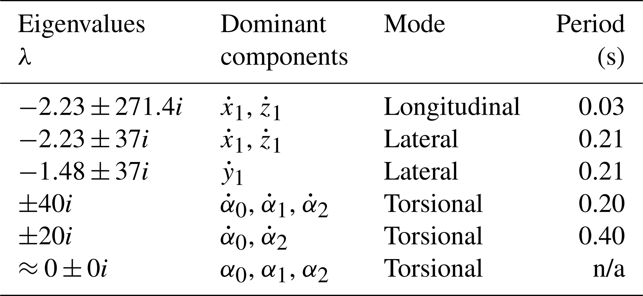
n/a: not applicable
5.2 Nominal operation of a RAWE machine with fixed ends
We now investigate the dynamic response of the helix when the torque at the upper end varies as
with mN0=2.88 and , which correspond to 25 N m and 2.6 s. For the controller in Eq. (40), we used and a target angular velocity of 120 rpm, which is the nominal value for the operation of the RAWE machine. Both ends of the structure are fixed according to the boundary conditions (35)–(36) and Eq. (66). The initial condition of the simulation is the stationary solution explained in Sect. 5.1. System (61) was integrated numerically with a Runge–Kutta algorithm and for N=2. Since the torques at the ends of the helix depend on time, the term in Eq. (56) involves the third derivative of α at s=0. For its evaluation at every time step during the numerical integration, we used backwards finite-difference approximations.
Figure 6a shows the evolution of for the three nodes of the structure (dotted, dashed, and solid lines) in the simulation. The controller successfully adjusted the torque on the ground (panel c) to make the structure rotate at the target angular velocity, which is 120 rpm. As shown in panel (b), the tension is almost constant throughout the helix and equal to around 200 N. The velocity of the nodes (not shown) tends to 0, and there is no lateral displacement. Therefore, the long-term state of the helix has its central line inside the xE−zE plane in a stationary condition, and the angles α for all the nodes rotate at a constant rate. The conclusions of this paragraph have been corroborated by running simulations with a higher number of elements (N=3 and N=5) and faster raising time of the torque at the upper end ( and ).
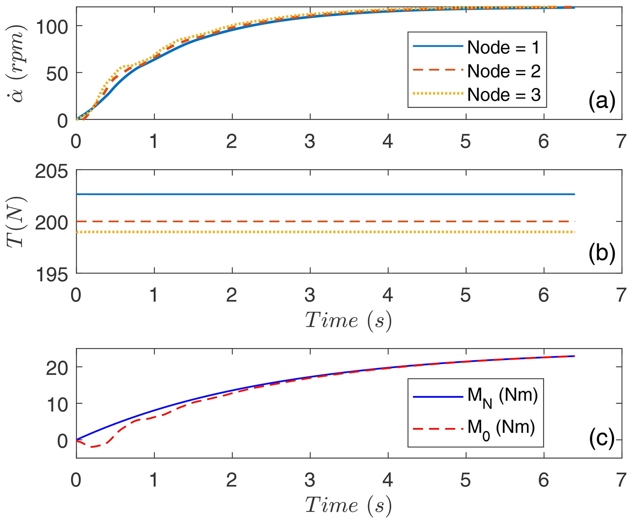
Figure 6Panels (a), (b), and (c) show the evolution of at the nodes and the target angular velocity (thick solid line), the torque at the ground, and the tensions at the nodes, respectively. The ends of the structure are fixed.
5.3 Dynamics of the RAWE machine with a mobile end
The real operation of a RAWE machine is more complex than the scenario described in Sect. 5.2 because the upper-end point is mobile. Although an auxiliary kite provides additional lift and helps to anchor it, the motion of the rotor and wind fluctuations naturally drive a motion for the upper end of the structure. This mechanism injects energy into the helix, and, as shown below, its dynamics depend heavily on the characteristic frequency of the forcing. Insight into the behavior of the RAWE machine can be obtained by using the model of this work and still avoiding the coupling with a rotor by considering the following boundary condition for the upper end:
It corresponds to a circular motion of the upper point of the structure with a radius and a frequency of R1=r1L0 and , respectively. Its effect on the dynamics of the structure has been studied experimentally and numerically.
The experiment, which was carried out inside the laboratory, used a structure with the characteristics in Tables 1 and 4. Although similar to the one considered in Sect. 5.2, we used a structure with a shorter length and lower mass due to space constraints in the laboratory. The nominal tension was also lowered to 80 N, and, according to Fig. 4 and Eq. (64), the bending stiffness is also lower (EI=6483 N m2). The nominal tension was adjusted by imposing an adequate distance between the tips of the structure. For this test, the torque was applied into the helix at the ground by a motor that was operated at a steady angular velocity. To impose the circular periodic motion given by Eq. (70), the helix’s upper-end point was attached to an eccentric arm that was powered with a second motor (see Fig. 2e). A radius of R1=0.1 m was used, and the frequency f1 was varied. An electromagnetic brake countered the torque on the eccentric arm. This is opposite to how the system operates in the generation mode of a RAWE machine, where the torque is generated by the rotor and countered by the generator on the ground. Nonetheless, the resulting torque in the helix during the experiment was the same as in a normal operation, and this experimental configuration avoided the need for having another motor with its power supply on the arm. Regarding diagnostics, the axial tension on the helix was measured with load cells on the attachment points at the ground.
Table 4Parameters used in the analysis of solutions with a mobile end.
As shown in Fig. 7, the frequency f1 of the eccentric arm was increased in multiple steps, and the total tension on the structure was measured with load cells. The lateral displacement of the helix was also monitored by using multiple cameras. The experimental data revealed that the tension oscillated at a frequency close to the driving frequency. The oscillations are regular for low frequencies and irregular for a driving frequency close to 5 Hz. It was also observed in the experiment that the amplitude of the oscillations, i.e., the lateral displacement of the central point of the structure, increased with the driving frequency. When the driving frequency reached 5 Hz, the structure collapsed because multiple tethers ripped, and the experiment was stopped. Interestingly, and as shown in Fig. 7, changing the forcing frequency from 0.7 to 2.1 Hz did not result in an enhancement of the tension. Only when the frequency was increased with up to 3.5 Hz and beyond were higher values measured by the load cells. According to these experimental results and the simulation results presented below, we conclude that the periodic forcing of the upper end induced a resonance in the structure. The irregular oscillations observed at high frequencies are a signature of the nonlinearities excited by the high values of the tension. They reached values equal to 3 times the nominal tension before the helix collapsed. We also mention that the frequency that produced the collapse (5 Hz) is of the order of the natural lateral and torsional frequencies of the helix. For the helix in Table 3, which has slightly different physical properties (compare Tables 2 and 4), the natural frequencies of the lateral and torsional modes are 1/0.2 s = 5 Hz and 1/0.4 s = 2.5 Hz. This result highlights the importance of having access to numerical tools for predicting the natural frequencies of the helix.
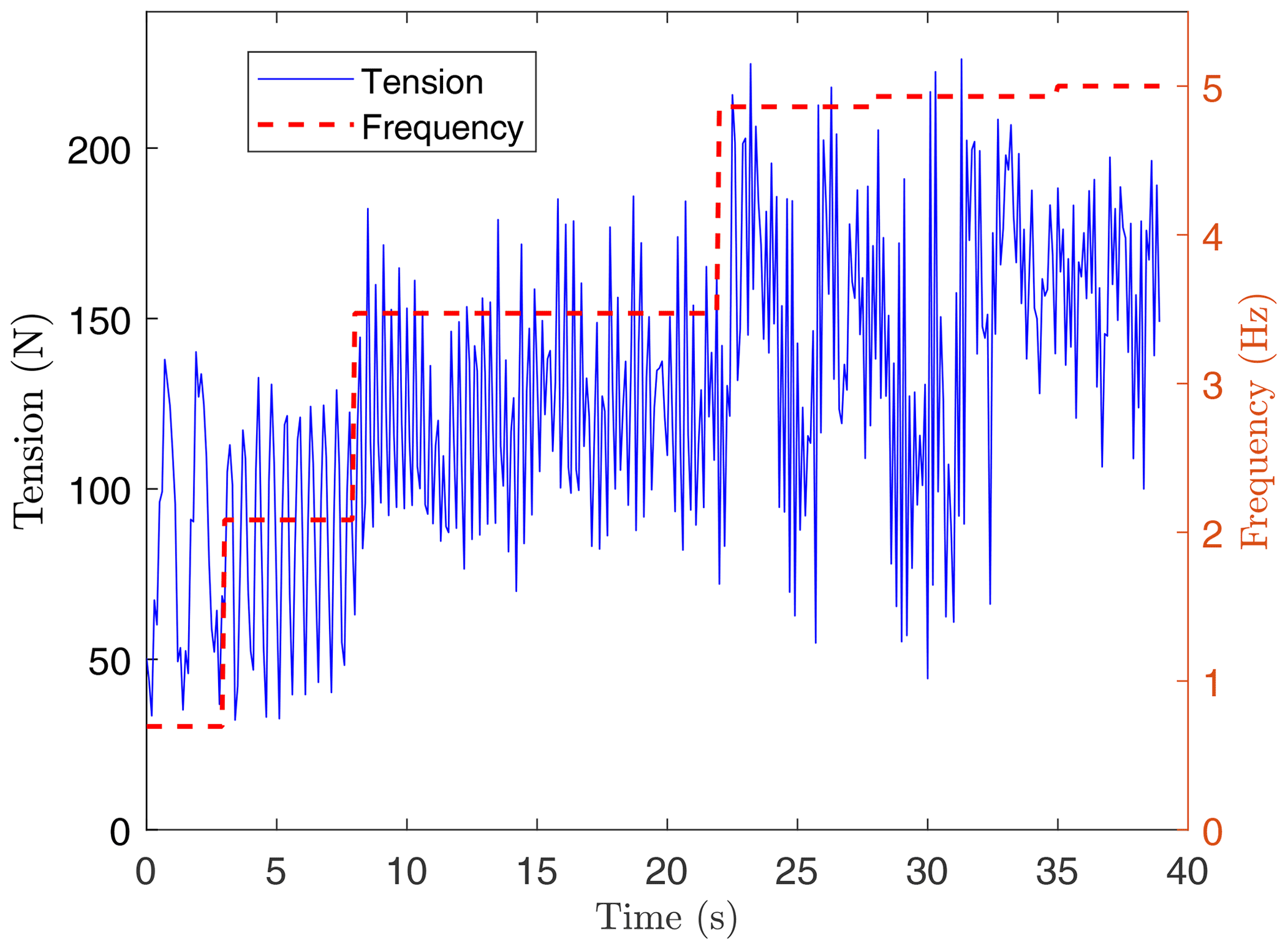
Figure 7Evolution of the tension (left) and the forcing frequency f1 (right) in the experiment with a mobile upper end.
The same scenario was also studied by using the simulator. Besides the parameters in Tables 1 and 4, we imposed the boundary condition given in Eq. (70) and set N=2. We started the analysis at a very low forcing frequency, and, for the initial condition, we used the procedure explained in Sect. 5.1. System (61) was then integrated numerically until the helix exhibited regular oscillations. The output tension at s=0 was then post-processed to identify its maxima (Tmax) in the long term (once the transient phase died out). Afterwards, the value of f1 was increased, and the full process was repeated but now using as initial condition the state of the helix at the end of the previous simulation.
The result of the analysis is the bifurcation diagram with Tmax versus f1 shown in Fig. 8. Interestingly, it brings out the strengths and weakness of the numerical tool. Regarding the former, the simulator predicts a resonance of the structure similar to the one observed in the experimental data. However, the maximum tension in the simulator rises for driving frequencies above around 9 Hz, whereas in the experiment an enhancement of the tension was detected for lower frequencies (above 3.5 Hz). The inset of Fig. 8 shows the evolution of the tension at s=0 for f1=10 Hz in the long term (after the transient has died out). Similarly to the experimental results obtained for low frequencies, the tension oscillates regularly and at a frequency close to f1. However, unlike the experimental data, the amplitude of the oscillations in the tension are small (a few newtons), whereas in the experiment they were of the order of tens of newtons. We also mention that the actual version of the simulator assumes that every cross section of the helix is unshearable. Therefore, the simulator cannot be used to predict the collapse of the helix. In fact, taking into account that the maximum tension in the experiment was about 200 N, it is likely that in the experiment we only observed the initial rise of the resonance curve shown in Fig. 8. For a tension of about 200 N, the driving frequency is about 11 Hz in Fig. 8.
Therefore, we conclude that the numerical tool is able to capture some interesting phenomena correctly, and it can be used to predict them qualitatively. However, if the interest is in getting quantitative values, then it should be used carefully. This conclusion is reasonable because the simulator relies on a set of simplifying hypotheses and also needs to be fed with inputs that have a certain level of uncertainty. As shown by the results of the experimental characterization of the structure in Sect. 4, the bending and torsional stiffness of the tensegrity structure is difficult to model. The stiffness depends on the tension and, in the case of torsional stiffness, it presents hysteresis. Since such hysteresis was found in the experiments, the results of this work open the question on how to incorporate such a phenomenon into the structural model. Theoretical models based on additional ordinary differential equations and artificial neural networks to fit complex hysteretic behaviors are two potential approaches. Interestingly, the former has recently been used in AWE to model the dynamic stall (Castro-Fernandez et al., 2024), which is another hysteretic phenomenon but in this case on unsteady aerodynamics. Another important topic is the modeling of the damping in the system, which could be improved in future work. The aerodynamic drag, already considered in the model, dissipates energy, but there are other mechanisms that may also be included. An example is the friction between elements of the tensegrity structure, which can affect the response of the system shown in Fig. 8. Consequently, the predictive capability of simulations is limited. Nonetheless, each simulation for a given f1 has a relatively low computational cost (around 1 min). This opens the possibility to perform analysis varying the physical parameters that are difficult to estimate and tune them in the simulator to reproduce the experimental results quantitatively.
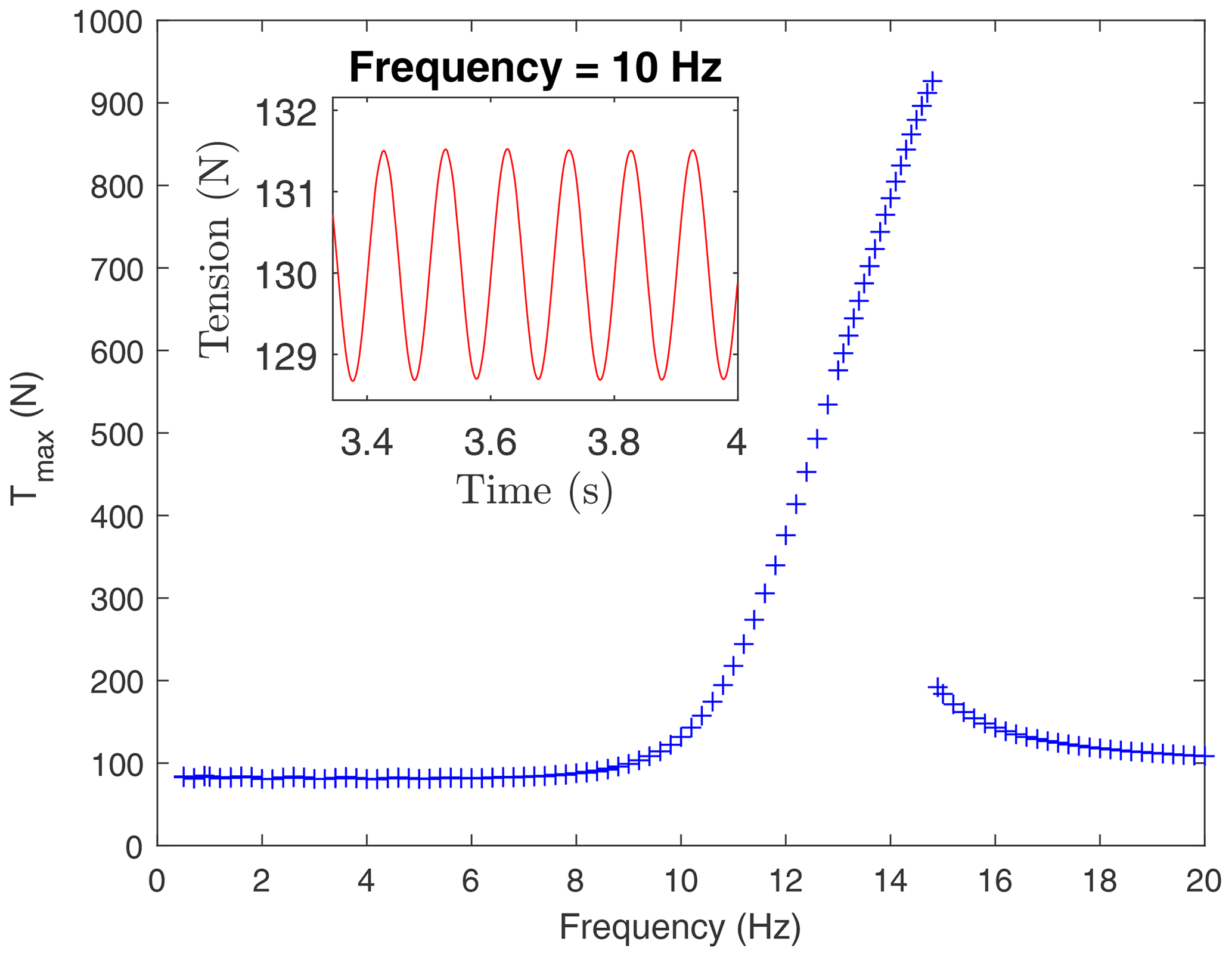
Figure 8Maximum values of the tension at s=0 versus the forcing frequency in the simulations. The inset shows the evolution of the tension at s=0 for the forcing frequency f1= 10 Hz.
The results of this work show that the proposed model based on Cosserat theory is appropriate for getting insight into the dynamics of the helical structure of a RAWE machine. It offers some advantages as compared to previous models based on springs and disks or a large set of masses linked with springs and dampers. For instance, unlike previous models, our model captures the three interesting motions of the helix, thus improving the fidelity. It provides a couple of nonlinear partial differential equations that can be solved with well-known numerical methods like the finite-element method used in this work. Such a compact formulation, which includes stretching, bending, and torsional effects, highlights the role of the different terms in the dynamics of the structure and their coupling. It has also been used here to estimate the characteristic times for the propagation of longitudinal, lateral, and torsional waves in the helix. Moreover, the airborne rotor and the ground generator enter the model as boundary conditions that include the position and velocity of the end sections of the structures and the external torque applied to them. The model was completed with the axial, bending, and torsional stiffness of a real AWE machine obtained by conducting three dedicated experiments in the laboratory. Since axial, bending, and torsional stiffness is essential information for RAWE machine simulators, such experimental work fills an important gap in the field. The relation between the bending and the torsional stiffness and the tension was measured for the tensegrity structure. It was also shown that the torsional stiffness depends on both the tension without torsion and the history of the structure as the tension is increased. A hysteric behavior was measured, which poses a challenge for the modeling of the helix.
The analysis of the stationary solution with no torsion and fixed ends, which was found independently by using a shooting algorithm, allowed us to verify the correct implementation of the finite-element code. A linear stability analysis was performed to identify longitudinal, lateral, and torsional modes and their natural periods. The quickest mode of the RAWE machine of SomeAwe corresponds to a longitudinal mode with a period of 0.03 s, whereas lateral and torsional modes exhibit natural oscillations with 0.2 and 0.4 s. Therefore, the natural frequencies of the helix predicted by the simulator are 33.3, 5, and 2.5 Hz. Simple estimations based on classical results for beams are in agreement with these results and constitute a second test for the correct implementation of the code.
The simulation tool provided interesting information about the nominal operation of the RAWE machine like the transient of the angular velocities of the cross sections of the helix, the tension, and the torques. A numerical analysis was carried out by keeping the two end points of the structure fixed. It assumed that the rotor imposes a time-dependent external torque that approaches 25 N m, which is a typical value for the RAWE machine under consideration. It was shown that a simple proportional-derivative controller for the torque at the ground generator can stabilize the angular spinning velocity of the structure at the target value (120 rpm). For this configuration, the tension is almost constant in time and throughout the structure. The evolution of the variables and their values are well aligned with the data collected in field testing by SomeAWE Labs.
In a second numerical analysis, the lower end of the helix was kept fixed, and the upper end was mobile. Although an auxiliary kite is used to anchor the rotor, in a real RAWE machine the upper-end point is not fixed due to wind velocity fluctuations and the dynamic coupling of the structure and the rotor. This scenario was mimicked by imposing a circular periodic motion to the upper end of the structure with a forcing frequency f1 and small amplitude. The experimental and simulation work revealed that there is a resonance that, in the case of the experiment, resulted in the collapse of the structure for a frequency of 5 Hz and for a tension level of about 200 N. The simulator captured essential features of the experiment, like the resonance and the order of magnitude of the critical frequency. The simulator cannot reproduce the collapse of the structure because the model was constructed by assuming that the cross sections of the helix are unshearable. For this reason, it was able to explore higher frequencies and tension values with the simulator, reaching a maximum above 900 N.
By assuming that the first derivative is continuous across the elements, we find the following relation between and (Press et al., 1992):
with
and we used the boundary conditions . For α, the continuity condition for α′ across the elements gives
with
where we used the boundary conditions and .
The code presented in this work was added as an independent module to the open-source software LAKSA (https://doi.org/10.5281/zenodo.11390955, Sánchez-Arriaga and Pastor-Rodriguez, 2017).
The data that support the findings of this study are available on request from author Christof Beaupoil (christof.beaupoil@gmail.com).
The model of the RAWE machine was developed by GSA and ACV. The implementation of the code, the numerical analysis, and the preparation of the manuscript were performed by GSA. DU and CB performed the experiments to characterize the RAWE machine in static and dynamic conditions. All the authors contributed to the discussion of the results and the final version of the paper.
Gonzalo Sánchez-Arriaga, Álvaro Cerrillo-Vacas, and Daniel Unterweger declare that they have no conflict of interest. Christof Beaupoil is the founder and owner of SomeAWE Labs.
Publisher’s note: Copernicus Publications remains neutral with regard to jurisdictional claims made in the text, published maps, institutional affiliations, or any other geographical representation in this paper. While Copernicus Publications makes every effort to include appropriate place names, the final responsibility lies with the authors.
This work was carried out under the framework of the GreenKite-2 project (grant no. PID2019-110146RB-I00) funded by MCIN/AEI/10.13039/501100011033.
This paper was edited by Alessandro Croce and reviewed by three anonymous referees.
Archer, C. L. and Caldeira, K.: Global Assessment of High-Altitude Wind Power, Energies, 2, 307–319, https://doi.org/10.3390/en20200307, 2009. a
Beaupoil, C.: Rotary Airborne Wind Energy Systems with Ground Based Power Generation: Overview and Practical Experiences, in: Airborne Wind Energy Conference 2017, Freiburg, 5–6 October 2017, edited by: Diehl, M., Leuthold, R., and Schmehl, R., 188 pp., https://doi.org/10.6094/UNIFR/12994, 2017. a
Beaupoil, C.: Airborne Wind Energy System with Tensile Rotary Power Transmission test run, https://www.youtube.com/watch?v=54zM3RC1Xoo&t=96s (last access: 29 October 2022), 2022. a
Beaupoil, C.: AWEC2019: Practical Experiences With a Torsion Based Rigid Blade Rotary Airborne Wind Energy System With Ground Based Power Generation, https://someawe.org/?p=343 (last access: 1 April 2024), 2024. a
Benhaiem, P. and Schmehl, R.: Airborne Wind Energy Conversion Using a Rotating Reel System, Green Energy Technol., 539–577, https://doi.org/10.1007/978-981-10-1947-0_22, 2018. a
Blanch, M., Makris, A., and Valpy, B.: Getting airborne – the need to realise the benefits of airborne wind energy for net zero, White Paper for Airborne Wind Europe, 44 pp., https://www.google.com/search?client=firefox-b-d&q=Getting+airborne+%E2%80%93+the+need+to+realise+the+benefits+of+airborne+wind+energy+for+net+zero (last access: 23 May 2024), 2022. a
Buckham, B. J.: Dynamics Modelling of Low-Tension Tethers for Submerged Remotely Operated Vehicles, PhD thesis, B. Eng. University of Victoria, 2003. a, b
Castro-Fernandez, I., Cavallaro, R., Schmehl, R., and Sánchez-Arriaga, G.: Unsteady aerodynamics of delta kites for airborne wind energy under dynamic stall conditions, Wind Energy, accepted, 2024. a
Cherubini, A., Papini, A., Vertechy, R., and Fontana, M.: Airborne Wind Energy Systems: A review of the technologies, Renew. Sust. Energ. Rev., 51, 1461–1476, https://doi.org/10.1016/j.rser.2015.07.053, 2015. a
De Schutter, J., Leuthold, R., and Diehl, M.: Optimal Control of a Rigid-Wing Rotary Kite System for Airborne Wind Energy, in: 2018 European Control Conference, European Control Conference (ECC), Limassol, Cyprus, 12–15 June 2018, 1734–1739, ISBN 978-3-9524-2698-2, 2018. a
European Commission: Study on challenges in the commercialisation of airborne wind energy systems, European Commission, https://op.europa.eu/en/publication-detail/-/publication/a874f843-c137-11e8-9893-01aa75ed71a1/language-en (last access: 29 May 2024), 2018. a
Love, A.: A Treatise on the Mathematical Theory of Elasticity, in: A Treatise on the Mathematical Theory of Elasticity, University Press, ISBN 9780486601748, 1944. a
Mackertich, S. and Das, T.: A quantitative energy and systems analysis framework for airborne wind energy conversion using autorotation, in: 2016 American Control Conference (ACC), Boston, 6–8 July, 4996–5001, https://doi.org/10.1109/ACC.2016.7526145, 2016. a
Malz, E. C., Walter, V., Goransson, L., and Gros, S.: The value of airborne wind energy to the electricity system, Wind Energy, 25, 281–299, https://doi.org/10.1002/we.2671, 2022. a
Motro, R.: Tensegrity: Structural Systems for the Future, Butterworth-Heinemann, ISBN 9781903996379, 2003. a
Njiri, J. G. and Soffker, D.: State-of-the-art in wind turbine control: Trends and challenges, Renew. Sust. Energ. Rev., 60, 377–393, https://doi.org/10.1016/j.rser.2016.01.110, 2016. a
Pfister, J.-L. and Blondel, F.: Comparing blade-element theory and vortex computations intended for modelling of yaw aerodynamics of a tethered rotorcraft, in: Science of Making Torque from Wind (TORQUE 2020), PTS 1–5, Journal of Physics Conference Series, Vol. 1618, ISSN 1742-6588, https://doi.org/10.1088/1742-6596/1618/3/032012, 2020. a
Press, W. H., Teukolsky, S. A., Vetterling, W. T., and Flannery, B. P.: Numerical Recipes, in: FORTRAN: The Art of Scientific Computing, 2nd edn., Cambridge University Press, USA, ISBN 052143064X, 1992. a
Ramézani, H., Jeong, J., and Feng, Z.-Q.: On parallel simulation of a new linear Cosserat elasticity model with grid framework model assumptions, Appl. Math. Model., 35, 4738–4758, https://doi.org/10.1016/j.apm.2011.03.054, 2011. a
Rancourt, D., Bolduc-Teasdale, F., Bouchard, E. D., Anderson, M. J., and Mavris, D. N.: Design space exploration of gyrocopter-type airborne wind turbines, Wind Energy, 19, 895–909, https://doi.org/10.1002/we.1873, 2016. a
Read, R.: Kite Networks for Harvesting Wind Energy, Springer Singapore, Singapore, 515–537, ISBN 978-981-10-1947-0, https://doi.org/10.1007/978-981-10-1947-0_21, 2018. a
Riahi, A. and Curran, J. H.: Full 3D finite element Cosserat formulation with application in layered structures, Appl. Math. Model., 33, 3450–3464, https://doi.org/10.1016/j.apm.2008.11.022, 2009. a
Rimkus, S. and Das, T.: An Application of the Autogyro Theory to Airborne Wind Energy Extraction, ASME 2013 Dynamic Systems and Control Conference, DSCC 2013, Vol. 3, https://doi.org/10.1115/DSCC2013-3840, 2013. a
Roberts, B. W., Shepard, D. H., Caldeira, K., Cannon, M. E., Eccles, D. G., Grenier, A. J., and Freidin, J. F.: Harnessing High-Altitude Wind Power, IEEE T. Energy Conver., 22, 136–144, https://doi.org/10.1109/TEC.2006.889603, 2007. a
Salma, V., Friedl, F., and Schmehl, R.: Improving reliability and safety of airborne wind energy systems, Wind Energy, 23, 340–356, https://doi.org/10.1002/we.2433, 2020. a
Sánchez-Arriaga, G. and Pastor-Rodriguez, A.: LAgrangian Kite SimulAtors (LAKSA), GitHub [code], https://doi.org/10.5281/zenodo.11390955, 2017.
Schelbergen, M., Kalverla, P. C., Schmehl, R., and Watson, S. J.: Clustering wind profile shapes to estimate airborne wind energy production, Wind Energ. Sci., 5, 1097–1120, https://doi.org/10.5194/wes-5-1097-2020, 2020. a
Schmehl, R.: Springer, Singapore, ISBN 978-981-10-1947-0, https://doi.org/10.1007/978-981-10-1947-0, 2018. a
Sommerfeld, M., Dörenkämper, M., Steinfeld, G., and Crawford, C.: Improving mesoscale wind speed forecasts using lidar-based observation nudging for airborne wind energy systems, Wind Energ. Sci., 4, 563–580, https://doi.org/10.5194/wes-4-563-2019, 2019. a
Sommerfeld, M., Dörenkämper, M., De Schutter, J., and Crawford, C.: Impact of wind profiles on ground-generation airborne wind energy system performance, Wind Energ. Sci., 8, 1153–1178, https://doi.org/10.5194/wes-8-1153-2023, 2023. a
Sánchez-Arriaga, G., García-Villalba, M., and Schmehl, R.: Modeling and dynamics of a two-line kite, Appl. Math. Model., 47, 473–486, https://doi.org/10.1016/j.apm.2017.03.030, 2017. a
Sánchez-Arriaga, G., Pastor-Rodríguez, A., Sanjurjo-Rivo, M., and Schmehl, R.: A lagrangian flight simulator for airborne wind energy systems, Appl. Math. Model., 69, 665–684, https://doi.org/10.1016/j.apm.2018.12.016, 2019. a
Tulloch, O., Kazemi Amiri, A. M., Yue, H., Feuchtwang, J., and Read, R.: Tensile rotary power transmission model development for airborne wind energy systems, J. Phys. Conf. Ser., 1618, 032001, https://doi.org/10.1088/1742-6596/1618/3/032001, 2020. a, b
Tulloch, O., Yue, H., Kazemi Amiri, A. M., and Read, R.: A Tensile Rotary Airborne Wind Energy System-Modelling, Analysis and Improved Design, Energies, 16, 1–42, https://doi.org/10.3390/en16062610, 2023. a
van de Kaa, G. and Kamp, L.: Exploring design dominance in early stages of the dominance process: The case of airborne wind energy, J. Clean. Prod., 321, 128918, https://doi.org/10.1016/j.jclepro.2021.128918, 2021. a
Villaggio, P.: Mathematical Models for Elastic Structures, Cambridge University Press, 162–302, ISBN 9780521017985, 2005. a
Wacker, J., McWilliam, M., Muskulus, M., and Gaunaa, M.: New model for structural optimisation of airborne wind energy systems with rotary transmission, J. Phys. Conf. Ser., 2626, 012011, https://doi.org/10.1088/1742-6596/2626/1/012011, 2023. a
- Abstract
- Introduction
- A model for rotary AWE machines
- A finite-element method
- Experimental characterization of the structure
- Dynamics of the helix: numerical and experimental results
- Conclusions
- Appendix A: Auxiliary calculations
- Code availability
- Data availability
- Author contributions
- Competing interests
- Disclaimer
- Financial support
- Review statement
- References