A new gridded offshore wind profile product for US coasts using machine learning and satellite observations

Offshore wind speed data around wind turbine hub heights are fairly limited, available through in situ observations from wind masts, sonic detection and ranging (sodar) instruments, or floating light detection and ranging (lidar) buoys at selected locations or as forecasting-model-based output from reanalysis products. In situ wind profiles have sparse geospatial coverage and are costly to obtain en masse, whereas satellite-derived 10 m wind speeds have vast coverage at high resolution. In this study, we show the benefit of deploying machine learning techniques, in particular random forest regression (RFR), over conventional methods for accurately estimating offshore wind speed profiles on a high-resolution (0.25°) grid at 6-hourly resolution from 1987 to the present using satellite-derived surface wind speeds from the National Oceanic and Atmospheric Administration (NOAA) National Centers for Environmental Information (NCEI) Blended Seawinds version 2.0 (NBSv2.0) product. We use wind profiles from five publicly available lidar datasets over the northeastern US and Californian coasts to train and validate an RFR model to extrapolate wind speed profiles up to 200 m. A single extrapolation model applicable to the coastal regions of the contiguous US and Hawai`i is developed instead of site-specific models attempted in previous studies. The model outperforms conventional extrapolation methods at the training locations as well as at two additional lidar and six National Offshore Wind (NOW)-23 stations that are independent of the training locations, especially under conditions of high vertical wind shear and at wind turbine hub heights (∼ 100 m). The final model is applied to the NBSv2.0 data from 1987 to the present to create 6-hourly wind speed profiles over the coastal regions of the contiguous US and Hawai`i on a 0.25° grid, which are shown to outperform NOW-23 and European Centre for Medium-Range Weather Forecasts (ECMWF) Reanalysis v5 (ERA5) at 100 m using a correlated triple-collocation method over 5 years of matchup data (2015–2019). Gridded maps of wind profiles in the marine boundary layer over US coastal waters will enable the development of a suite of wind energy resources and will help stakeholders in their decision-making related to wind-based renewable energy development.

1 Introduction

In 2023, the US offshore wind energy potential capacity grew to ∼ 53 GW (Musial et al., 2023). This includes operational projects, wind farms under construction, and those which are in various other stages of development. Planning an offshore wind farm requires finding an optimal location that fulfills different requirements, including pricing, optimized siting, regulation, and grid integration, among others. For these efforts, stakeholders in the wind energy industry need a suite of wind resources, including a wind atlas that will examine the wind at various heights from the ocean surface up to wind turbine hub heights. A long-term, stable database of wind speeds is a particularly pressing need for the wind energy sector, not only at commonly used hub heights of ∼ 100 m (with a rotor diameter of ∼ 90 m), but also at higher hub heights of ∼ 140 to 160 m, as continued technological improvements allow for larger wind turbines and for the full rotor layer of the turbines to enable accurate calculations of rotor-equivalent wind speed.

The biggest hindrance to developing such a long-term database is the scarcity of accurate wind speed observations within the rotor layer of wind turbines. Wind speeds at these heights are often measured by meteorological towers in coastal areas. This becomes less cost-effective as newer, larger turbines are developed since the price of measurements increases with height. Sonic detection and ranging (sodar) instruments can measure wind speed by taking advantage of the Doppler shift phenomenon. Sodars, though portable, provide wind speeds and directions from 30 m to up to 200 m at a 5 m resolution; however, these measurements are very site-specific (Hanson 2006; He et al., 2022), can potentially have lower accuracies, and are prone to high background noise and solid reflection (Peña et al., 2013). Buoy-mounted floating light detection and ranging (lidar) instruments provide an alternative way to measure winds at those heights but are equally expensive and available for particular sites only. In addition, lidar measurements can be limited by challenging environments or inclement conditions and have difficulty accounting for the effects on wind speed observations due to the movement of waves in the ocean (Clifton et al., 2018). However, due to their lower maintenance cost, they are commonly used by wind farm developers. As most of these lidar data are not publicly available due to proprietary reasons, there remains a scarcity of wind speed observations within the rotor layer of turbines. The only data that are publicly available are from a few lidar stations and the 2023 National Renewable Energy Laboratory (NREL) National Offshore Wind (NOW)-23 dataset that is based on the Weather Research and Forecasting (WRF) model in and around the coastal US (Bodini et al., 2023), as described in Sect. 2. Since the few publicly available lidar stations have limited spatio-temporal coverage and NOW-23 only spans ∼ 20 years, there is a gap in real-time wind speed profile knowledge along the US coasts. Satellite-based products can be utilized to develop wind speed profile gridded datasets with vast coverage and high resolution that can help address this critical database gap. Using the National Oceanic and Atmospheric Administration (NOAA) National Centers for Environmental Information (NCEI) Blended Seawinds version 2 (NBSv2.0) product, we derive vertical wind speed profiles around US coasts from July 1987 to the present, providing ∼ 38 years of historical data with near-real-time data (1 d latency) and science-quality data updated monthly.

This issue of extrapolating existing wind speed observations from a small number of heights to full wind speed profiles has received significant attention by many previous studies. The buoy-based wind speed (hereafter, “surface” wind speed) measurements from the National Data Buoy Center, maintained by NOAA (NOAA National Data Buoy Center, 1971), have been used previously, along with satellite-based surface wind data, to estimate winds at the turbine rotor-swept heights (Doubrawa et al., 2015; Optis et al., 2020a, 2020b). However, these studies used either conventional extrapolation techniques or industry-accepted wind models like the Wind Atlas Analysis and Application Program (WAsP) and are very region-specific.

Several studies have estimated wind profiles from the surface up to turbine rotor-swept heights using various machine learning techniques, but most of these are site-specific case studies, where lidar measurements were used to train and develop the respective models (e.g., Mohandes and Rehman, 2018; Bodini and Optis, 2020a; Optis et al., 2021). A study using 2 years of wind mast and modeled mesoscale data below 80 m from the New European Wind Atlas (NEWA) to extrapolate 102 m wind speeds showed that multiple machine learning methods, including linear, ridge, lasso, elastic net, support vector, decision tree, and random forest regression (RFR), outperformed the power law, with RFR performing the best, with an increase in the coefficient of determination (R²) of 42 % compared to the power law (Baquero et al., 2022). Over a land-based site in China, the RFR outperformed the power law in extrapolating wind speeds at 120, 160, and 200 m (Liu et al., 2023). At four land-based stations in Oklahoma, the RFR outperformed both the logarithmic and the power-law-based extrapolation, improving accuracy by 25 % when trained and validated at the same site and by 17 % when using a round-robin approach where cross validation was performed by leaving out one station from training at a time for validation (Bodini and Optis, 2020a). In addition, the RFR was able to extrapolate wind profiles during low-level jet (LLJ) occurrences at the four land-based stations, showing improved performance over the logarithmic method, which is unable to replicate such events where surface winds decouple from winds aloft (Optis et al., 2021). LLJs are defined by their wind speed gradient inversion within the stable boundary layer and are important resources for offshore wind energy production along with other high-vertical-wind-shear events (Borvarán et al., 2021; Gadde and Stevens, 2021; Doosttalab et al., 2020). In many previous studies, machine learning methods have shown potential to more accurately estimate wind profiles compared to conventional methods, allowing for more informed decision-making for wind farm siting.

RFR in particular has shown promise in extrapolating wind profiles, specifically within the offshore environment. At the E05 Hudson North and E06 Hudson South stations, equipped with floating lidar buoys, the RFR outperformed the logarithmic formula, a single-column model, and the WRF model, with no evidence of decreased model performance under the same round-robin approach between the two buoys 83 km apart (Optis et al., 2021). As such, Optis et al. (2021) suggested that machine learning methods are promising for extrapolating 10 m satellite-resolved wind speeds in the relatively homogeneous offshore environment. In addition, they showed that including the difference between air temperature and sea surface temperature as input to the RFR greatly improved the model by quantifying atmospheric stability. Other work at the three German Forschung in Nord- und Ostsee (FINO1, FINO2, and FINO3) mast stations located in the North Sea and the Baltic Sea around Denmark also found the air–sea temperature difference to be an important input to the RFR (Hatfield et al., 2023). While machine learning has been used to improve wind extrapolation in a site-specific manner, we are unaware of any past studies that have used it over a large spatial scale covering multiple coasts, as done in our work.

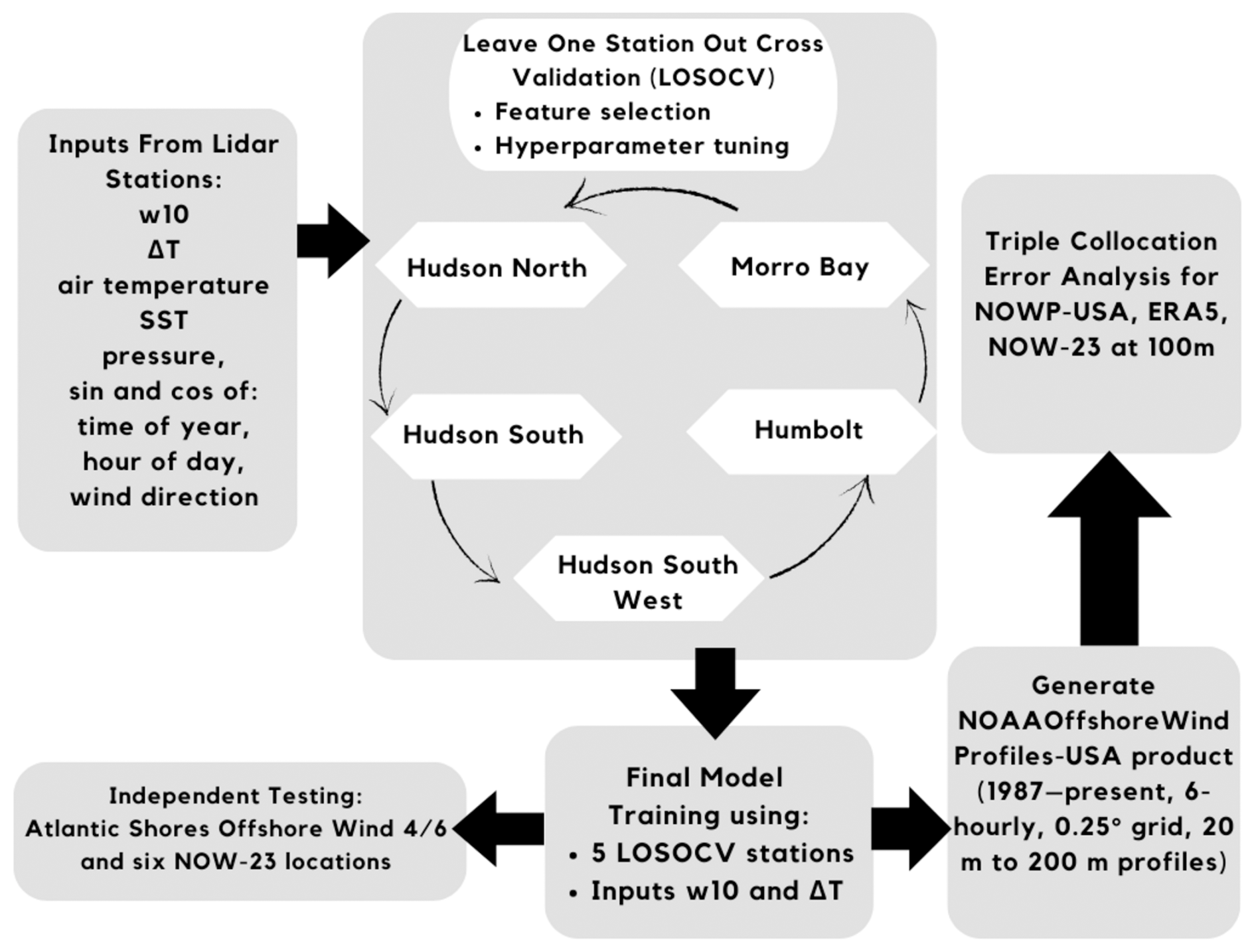
In this study, we apply an RFR developed using offshore lidar data to NBSv2.0 satellite-derived blended gap-free sea surface winds to generate a long-term (1987–present) product of wind speed profiles up to 200 m on a 0.25° grid around the coastal regions of the contiguous US and Hawai`i. Section 2 introduces the data used for training, validation, and testing of the extrapolation methods; Sect. 3 describes the conventional vertical wind extrapolation methods; Sect. 4 describes the RFR extrapolation model development; Sect. 5 compares the performance of the RFR and conventional methods on the training/validation data, both overall and specifically for LLJs and high-vertical-wind-shear events; Sect. 6 describes the independent testing of the extrapolation models; Sect. 7 introduces the new wind profile product, NOAAOffshoreWindProfiles-USA, and its error estimation at hub heights; and Sect. 8 summarizes our analysis and gives conclusions. A schematic overview of the methodology for generating the NOAAOffshoreWindProfiles-USA product is provided (Fig. 1).

Figure 1 A schematic overview of the methodology used in this analysis.

2 Data

2.1 Lidar stations

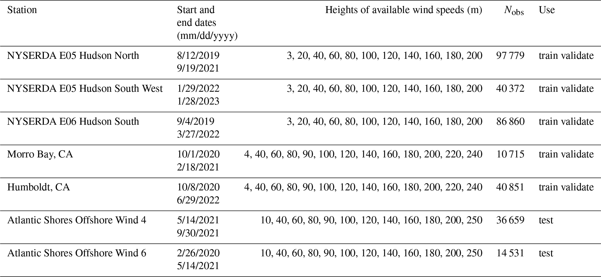
Data from five offshore lidar stations were used to train and validate the models in this analysis (locations shown in Fig. 2). Three stations (E05 Hudson North, E05 Hudson South West, and E06 Hudson South) are freely available from Ocean Tech Services/Det Norske Veritas (DNV) under contract to the New York State Energy Research and Development Authority (NYSERDA) and are located in the New York Bight call areas. The other two stations are on the Californian coast at Humboldt (Wind Data Hub, 2022a, 2022b) and Morro Bay (Wind Data Hub, 2020, 2021), and those data are freely available from the Wind Data Hub, funded by the Department of Energy. All lidar stations provide 10 min data, including surface wind speed, surface wind direction, wind profiles ranging between 40 and 200 m at intervals of 20 m, surface air temperature, sea surface temperature, and surface pressure, all of which are considered in this analysis. In total, there are 276 577 profiles spanning 10 min that are used to train and validate the model, with 35 % of the data coming from Hudson North, 31 % from Hudson South, 15 % from Hudson South West, 4 % from Morro Bay, and 15 % from Humboldt. Additional lidar buoy data from the Atlantic Shores Offshore Wind (ASOW) 4 and 6 stations were used as an independent test set that was not used in the model training or validation (Atlantic Shores Offshore Wind, 2023a, b, c, d). These included 14 531 and 36 659 profiles from ASOW-4 and ASOW-6, respectively, provided at 10 min intervals. Each of the seven stations provided data over a different time period within the range of August 2019 to January 2023 (Table 1).

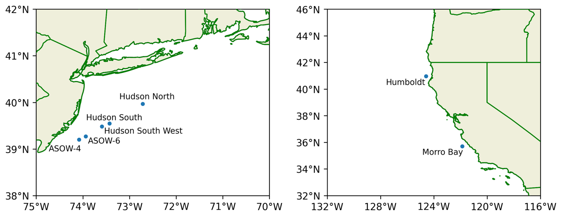
Figure 2 Locations of floating lidar buoy stations used for training, validating, and testing the random forest regression.

Table 1 Data availability of each lidar station used in this analysis.

2.2 NOAA/NCEI Blended Seawinds

The NOAA/NCEI Blended Seawinds v2.0 (NBSv2.0) product contains 10 m neutral winds and wind stresses globally gridded at a 0.25° spatial resolution dating back to July 1987 at 6-hourly, daily, and monthly resolution. Data from 17 satellites are blended to create the product, using up to 7 satellites at a given time, enabling the product to delineate extreme wind speeds with higher accuracy than other wind-based products (Saha and Zhang, 2022). The product is currently archived at NCEI (Saha and Zhang, 2023) and is available both in near-real time and in a science-quality (post-processed) format through NOAA CoastWatch. NBSv2.0 is a well-calibrated, uninterrupted, long-term, gap-free, and stable dataset. The 6-hourly data are used here as the input to generate the final gridded wind profile product.

2.3 Model and reanalysis data

The offshore wind industry widely uses wind profiles from the NREL Wind Integration National Dataset (WIND) Toolkit (Draxl et al., 2015a), which are available around the coastal US at high spatial and temporal resolution. The latest version of this dataset is the NREL NOW-23 reanalysis data (Bodini et al., 2023, 2024). This product is generated using the WRF numerical weather prediction (NWP) model with the European Centre for Medium-Range Weather Forecasts (ECMWF) Reanalysis v5 (ERA5) product as input to estimate wind profiles up to 500 m for US coastal regions beginning on 1 January 2000. NOW-23 data currently extend through 31 December 2019 for Hawai`i and the North Pacific regions, through 21 December 2022 for the South Pacific region (e.g., offshore California), and through 31 December 2020 in all other regions. The 2 km horizontal spatial resolution NOW-23 files are available at both 5 min and 1 h time resolution through the Open Energy Data Initiative program of the US Department of Energy via their Amazon Web Service (AWS) public data registry page. Another source of long-term wind speeds, at 10 and 100 m only, is the ERA5 product, which uses the Integrated Forecasting System (IFS) to produce hourly estimates on a 0.25° global grid dating back to 1940 (Hersbach et al., 2023). ERA5 2 m air temperature and sea surface temperature are also used to generate air–sea temperature differences (ΔT) as input to the RFR when implemented on NBSv2.0. These fields are downloaded using the Climate Data Store (CDS) Application Program Interface.

3 Conventional methods for wind extrapolation

3.1 Logarithmic law

Conventional physics-based models are typically implemented to vertically extrapolate surface winds, namely a logarithmic law and a power law. The logarithmic law is based on Monin–Obukhov similarity theory (Monin and Obukhov, 1954) and relates wind speed v to height z as follows:

$$\begin{array}{}\text{(1)}& v\left(z\right)={\displaystyle \frac{u_{\ast }}{K}}\left[\ln \left({\displaystyle \frac{z}{z_{\mathrm{0}}}}\right)-\mathit{\psi }\left({\displaystyle \frac{z}{L}}\right)+\mathit{\psi }\left({\displaystyle \frac{z_{\mathrm{0}}}{L}}\right)\right],\end{array}$$

where u_∗ is the friction velocity of the surface, K is the von Karman constant (usually 0.4), z₀ is the surface roughness, and ψ is a correction function for atmospheric stability that relies on the Obukhov length (L) (Holtslag et al., 2014). $\mathit{\psi }\left(\frac{z_{\mathrm{0}}}{L}\right)$ can usually be ignored as it tends to be minimal compared to $\mathit{\psi }\left(\frac{z}{L}\right)$ in an offshore environment. There are many different formulations for ψ, many of which only have applicability within a certain range of L. Much research has been done to compare the various different formulations and create new ones that have their own ranges of applicability (Essa, 2000; Holtslag et al., 2014; Jiménez et al., 2012; Optis et al., 2016; Schlögl et al., 2017). In addition to needing different formulations under certain conditions, the logarithmic law fails to accurately estimate wind profiles in conditions where surface winds decouple from winds aloft, namely in the presence of LLJs (Optis et al., 2021). As such, a more simplistic and accurate model is desired. The neutral logarithmic law removes the stability functions (assumes neutral stability) to give a simpler model but tends to have lower accuracy than other variations of the logarithmic law. The neutral logarithmic law finds wind speed v₂ at height z₂ by relating to a reference wind speed v₁ at height z₁ (Monin and Obukhov, 1954):

$$\begin{array}{}\text{(2)}& v_{\mathrm{2}}=v_{\mathrm{1}}{\displaystyle \frac{\ln \left(\frac{z_{\mathrm{2}}}{z_{\mathrm{0}}}\right)}{\ln \left(\frac{z_{\mathrm{1}}}{z_{\mathrm{0}}}\right)}}.\end{array}$$

Hereafter, we compare wind profiles extrapolated using the neutral logarithmic law to those from the RFR. Due to a lack of variables necessary for estimating the stability functions at the lidar stations, namely u_∗ and z₀, we were restricted to using the neutral logarithmic law. An estimate of z₀= 0.0001 was used in the absence of available data at the buoys (following Optis et al., 2021).

3.2 Power law

The power law for wind profile extrapolation relates wind speeds v₂ and v₁ at two heights z₂ and z₁, respectively, as

$$\begin{array}{}\text{(3)}& v_{\mathrm{2}}=v_{\mathrm{1}}{\left({\displaystyle \frac{z_{\mathrm{2}}}{z_{\mathrm{1}}}}\right)}^{\mathit{\alpha }},\end{array}$$

where α is the wind shear coefficient. When the wind speeds at two heights (z₁, z₂) are known, α can be computed directly from the two wind speeds:

$$\begin{array}{}\text{(4)}& \mathit{\alpha }={\displaystyle \frac{\ln \left(\frac{v_{\mathrm{2}}}{v_{\mathrm{1}}}\right)}{\ln \left(\frac{z_{\mathrm{2}}}{z_{\mathrm{1}}}\right)}},\end{array}$$

which in turn can be used to extrapolate the wind speeds at a third height in the given profile by substituting Eq. (4) (re-written for height 3 and either height 1 or height 2) for α in Eq. (3).

When wind speed is provided at only one height in a profile, α must be estimated to extrapolate wind speeds at subsequent heights. Over oceans, α can be estimated as a constant of 0.10 (Bañuelos-Ruedas et al., 2011). However, α is highly variable depending on the time of day, season, location, wind speed, and height; therefore, α should not be used as a constant and should instead be modeled as a parameter (Spera and Richards, 1979). Some studies focus on finding the best average estimate of α for a specific wind resource site (Gualtieri and Secci, 2011; Werapun et al., 2017). Others define formulations for α that account for the effects of wind speed and surface roughness (Spera and Richards, 1979) or for the effects of atmospheric stability by using correction functions based on Monin–Obukhov similarity theory (Panofsky and Dutton, 1984). While the addition of stability corrections into the formulation of α greatly increases the accuracy of a site-specific long-term average α, site-specific information on stability is necessary for this method, and it is rather sensitive to the surface roughness z₀ (Gualtieri, 2016). A time-varying model for α showed large increases in accuracy compared to previous models that used a site-specific α (Crippa et al., 2021). However, the model still relies on how α varies around a known specific α₀ for a given location or a predetermined constant value. Overall, there is no rule-of-thumb formulation for α that always best accounts for all of the factors that contribute to variability in α. In our power law estimates below (Sect. 5), we use an α value of 0.10, as suggested for the offshore environment (Bañuelos-Ruedas et al., 2011).

In addition, the power law has shown inconsistency when used for estimates of wind energy potential. Power law extrapolation using $\mathit{\alpha }=\mathrm{1}/\mathrm{7}$ underestimated wind power potential by approximately 40 % (Sisterson et al., 1983). In general, differences in wind energy production estimates when using a power law versus measured energy production may be up to 35 % (Werapun et al., 2017). Global median absolute percentage errors in onshore wind turbine capacity factor estimations are as large as 36.9 % when using α= 0.14 % and 5.5 % when using mean power law exponents (Jung and Schindler, 2021). As such, more accurate methods of vertically extrapolating wind speeds are critical for accurate representation of wind energy production.

4 Random forest regression (RFR) model training

Random forest regression (RFR) is a machine learning algorithm that takes an ensemble average of the predictions from its members, decision trees, to make one final prediction for each set of input data (Breiman, 2001). Each decision tree is trained on a bootstrapped subset (sampling with replacement) of the full training set, and each decision within the tree is made only considering a random subset of the input parameters (i.e., “features”) at each split to add variability to the structures of the trees. Both of these model architecture choices add “randomness” to the model. Each split is made by choosing the optimal value of one of the features available at that “branch” such that the data in that branch are split into two new branches, each with the smallest possible within-group variance. This process is continued until the branch contains a number of observations less than or equal to the hyperparameter (set by the user) for the minimum number of samples required to be at a branch node. Once this minimum sample size is reached, the branch is termed a “leaf” and is no longer split. We use the RandomForestRegressor function from the scikit-learn Python library for this analysis. By training each decision tree in the RFR on diverse subsets of the data and then averaging their predictions, it both increases accuracy and reduces overfitting.

The RFR model is trained to estimate wind speed profiles from 40 to 200 m at 20 m intervals. We chose to develop a single model to predict the entire profile to reduce the computation time needed, as compared to training different models for every height, but found identical performance in both cases. Inputs considered in the model for prediction are “surface” (10 m) wind speed (w₁₀), surface wind direction (θ), surface air temperature (T), sea surface temperature (SST), surface pressure, hour of day, time of year, and the difference between T and SST (ΔT) from the five lidar stations described above. The time of year was calculated as an index for the number of 10 min intervals (the training data resolution) in a year starting on 1 January at 00:00:00 UTC and ending on 31 December at 23:50:00 UTC. No information about latitude and longitude is included as input to the model, as we want our model to generalize well to many locations without knowing which location the input is coming from. As such, the model only learns the relationships between surface variables and wind profiles without linking specific relationships to given regions. Since the stations do not directly have 10 m wind speed available, w₁₀ was interpolated using the power law, with α calculated using the wind shear between the surface and the next lowest height available (20 m for Hudson stations, 40 m for Morro Bay and Humboldt). The cyclical features (wind direction, hour of day, and time of year) were decomposed into sine and cosine components to preserve their cyclical nature (i.e., to ensure 23:00 UTC is equally close to 22:00 UTC as it is to midnight), consistent with the treatment of such variables in previous RFR studies (e.g., Sharp et al., 2022). Only time and surface variables are included as inputs in our model, but other studies (Liu et al., 2023; Bodini and Optis, 2020a; Baquero et al., 2022) included variables at several heights as inputs in their models. While inputs at other heights could further improve our model, these inputs would be unrealistic for implementation on a gridded wind profile product as no gridded products that contain observed wind speeds or other variables at those heights exist. Additionally, the training data do not contain any profile data other than the wind speeds (and wind direction at the Hudson stations only). Other surface variables, such as friction velocity, the Charnock coefficient, and sensible heat flux, have proved to be important features (Liu et al., 2023) and could potentially improve the model further, but these data are not available at the training stations used in this analysis.

A cross-validation method, in which each station was held out as a validation set for a model trained using the other stations, hereafter referred to as the leave-one-station-out cross validation (LOSOCV), was implemented during the model training to avoid overfitting to the training stations and to ensure the model's ability to generalize to unseen data, consistent with previous studies (Bodini and Optis, 2020a, b). In this LOSOCV approach, five different RFR models were constructed, and each time a different one of the five training/validation lidar sites was not included in the training dataset. After training an RFR on the other four sites' data, the input data from the validation site for that model were run through the RFR to assess its performance relative to the observed wind profiles at that location. The goal of this approach is to evaluate whether each model retains high performance at a location where the model has no prior knowledge of wind profiles. While the three Hudson stations may be close enough to one another that some prior knowledge of wind profiles in the area may be known in validating at those stations, the Californian stations are 631 km apart, so it is unlikely that there is prior knowledge of the wind profiles at either station within the model when validating at those stations.

Initially, five LOSOCV RFR models (each with all 11 features) were trained to validate performance at their respective hold-out station and to assess overall feature importance. It is important to optimize the input variables selected for the model by removing features that have a negative or negligible effect on the model's accuracy upon inclusion. This will maximize the model's accuracy while minimizing the computation time needed for training and parameter tuning as well as the number of inputs needed to generate our final product. To decide which features are important to keep, only features that clearly decrease the validation errors in the LOSOCV models at all locations are included. The average feature importance across all five models for each feature was evaluated during feature selection (Fig. 3). Both w₁₀ and ΔT had substantially higher feature importance than the other variables, so they were immediately selected for inclusion in the final model. While the other features had much smaller feature importance, a forward sequential feature selection process, where the improvement of the model from including each feature is assessed one feature at time, was used to determine if any of the remaining variables further minimized model errors. This process is important as significant cross correlations between the variables may not be reflected in the feature importance. Additional LOSOCV models were created using w₁₀, ΔT, and one of the remaining features, considered individually, with the sine and cosine components of each cyclical feature regarded as one feature in this process. At each hold-out station, the performance of these models was then compared to that of the LOSOCV models that only used w₁₀ and ΔT as inputs. If a model with three features showed smaller errors compared to the errors in the model with two features, that would indicate the additional feature was beneficial to include in the final model. This process was done recursively to identify all the features that improved the model. As none of the other features further reduced the errors over all hold-out stations (not shown here), the final model only uses w₁₀ and ΔT as inputs.

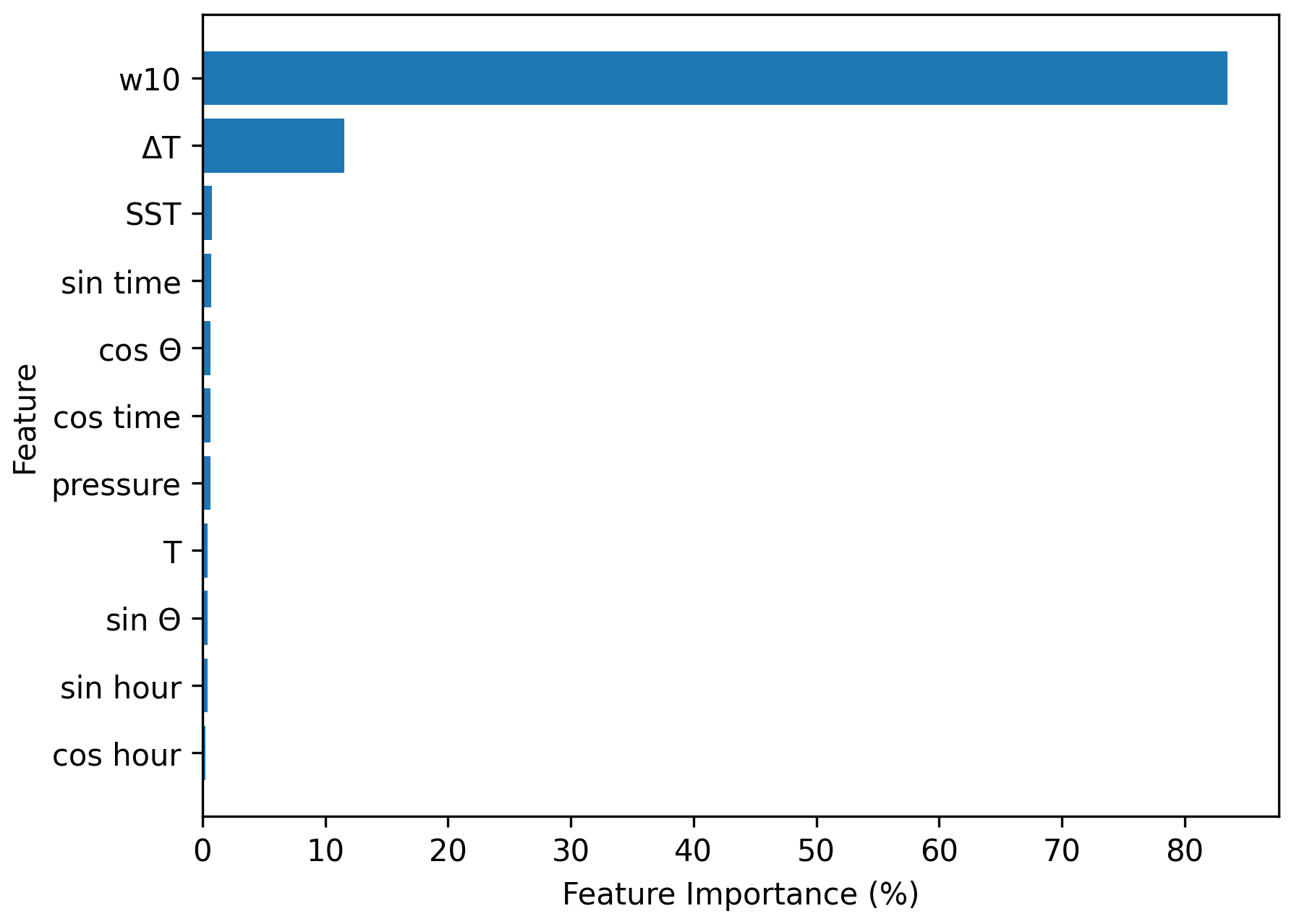
Figure 3 Average feature importance (over the five leave-one-station-out models) of the 11 input variables considered for the random forest regression model. Note that “time” refers to “time of year” as defined in the text.

Once w₁₀ and ΔT were chosen as features for the RFR model, the hyperparameters for the model were tuned. The process included tuning three hyperparameters: the number of features considered at each split, the minimum number of observations on each leaf, and the number of trees in the model (nTrees). The number of features to consider at each split could only be one or two as there are only two features in the final model. An essential part of the RFR is that not all features should be considered at each split to prevent the individual underlying decision trees from becoming too similar, which would remove randomness from the RFR (Breiman, 2001). Therefore, only one feature was considered for each split in our model. The minimum number of allowed observations on a given leaf is critical to tune because if it is too small, it will increase the depth of the trees, increasing the computation time and storage size of the model while potentially also overfitting the training data. If this hyperparameter is too large, it can result in an overly smoothed model that does not represent all the complexities of the training data. The number of trees in the model was tuned to minimize error in the model and avoid underfitting by averaging over too few trees. The optimal values for these two hyperparameters were determined by analyzing the out-of-bag (OOB) error, which corresponds to the average error when all the training observations not included in the bootstrapped subsample used to train a given tree are run through that tree for a pseudo-validation. Minimum leaf size values of 10, 15, 20, 30, 40, and 50 were evaluated for values of nTrees ranging from 20 to 2000 trees incrementing by 20 trees up to 100, followed by increments of 100 trees thereafter. A minimum leaf size of 30 minimized the error and is therefore chosen as the final hyperparameter value. We chose to use nTrees = 1000 trees as this is just above the nTrees value where the OOB error stabilizes, and any additional trees would not yield a further decrease in error but would simply increase computation time. These values were optimal for all five LOSOCV RFR models, which shows that these hyperparameters are not dependent on the locations of the training data.

After selecting the best features and tuning the hyperparameters for our model using our cross-validation process, we trained a final “optimal” RFR model on all five training/validation stations. This allowed us to use as much data as possible in the model in order to improve its accuracy and generalizability. This approach is consistent with other RFR-generated products (e.g., Sharp et al., 2022).

5 Extrapolation model performance on training/validation data

5.1 All wind conditions

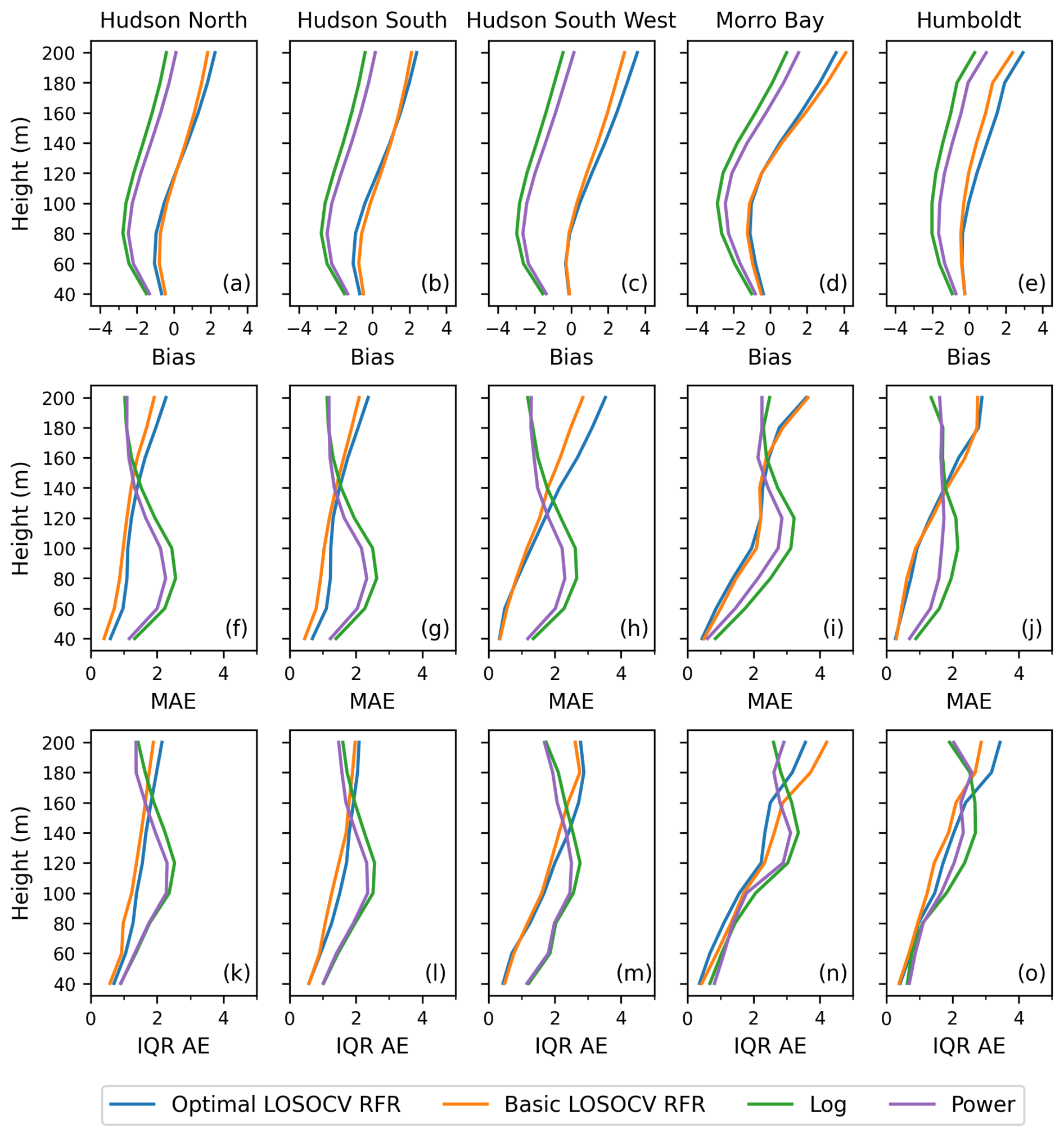
Three metrics were employed to assess the skill of our RFR model relative to the conventional physics-based models for wind profile extrapolation in all wind conditions: bias, median absolute error (MAE), and interquartile range of the absolute error (IQR AE). These metrics are obtained by comparing the observed lidar wind speeds and a given model's wind speed predictions (predicted minus observed) at every height for each station. Bias is used to determine whether or not the RFR overpredicts or underpredicts on average, MAE is used to give estimates of the typical magnitude of the error, and IQR AE determines a spread in the errors around the MAE. For each station and height, these metrics were computed on the validation data from each LOSOCV split for the “optimal” RFR (with w₁₀ and ΔT as features and the tuned hyperparameter values) and the “basic” RFR (with all 11 original features and no hyperparameter tuning), as well as for the neutral logarithmic law and the power law using α= 0.1 (Fig. 4). For the RFR models, the errors are calculated using the LOSOCV approach discussed previously, ensuring the errors at a given validation site are calculated from the LOSOCV RFR model with no prior knowledge of the wind conditions at that site so as to best represent the model's generalization error.

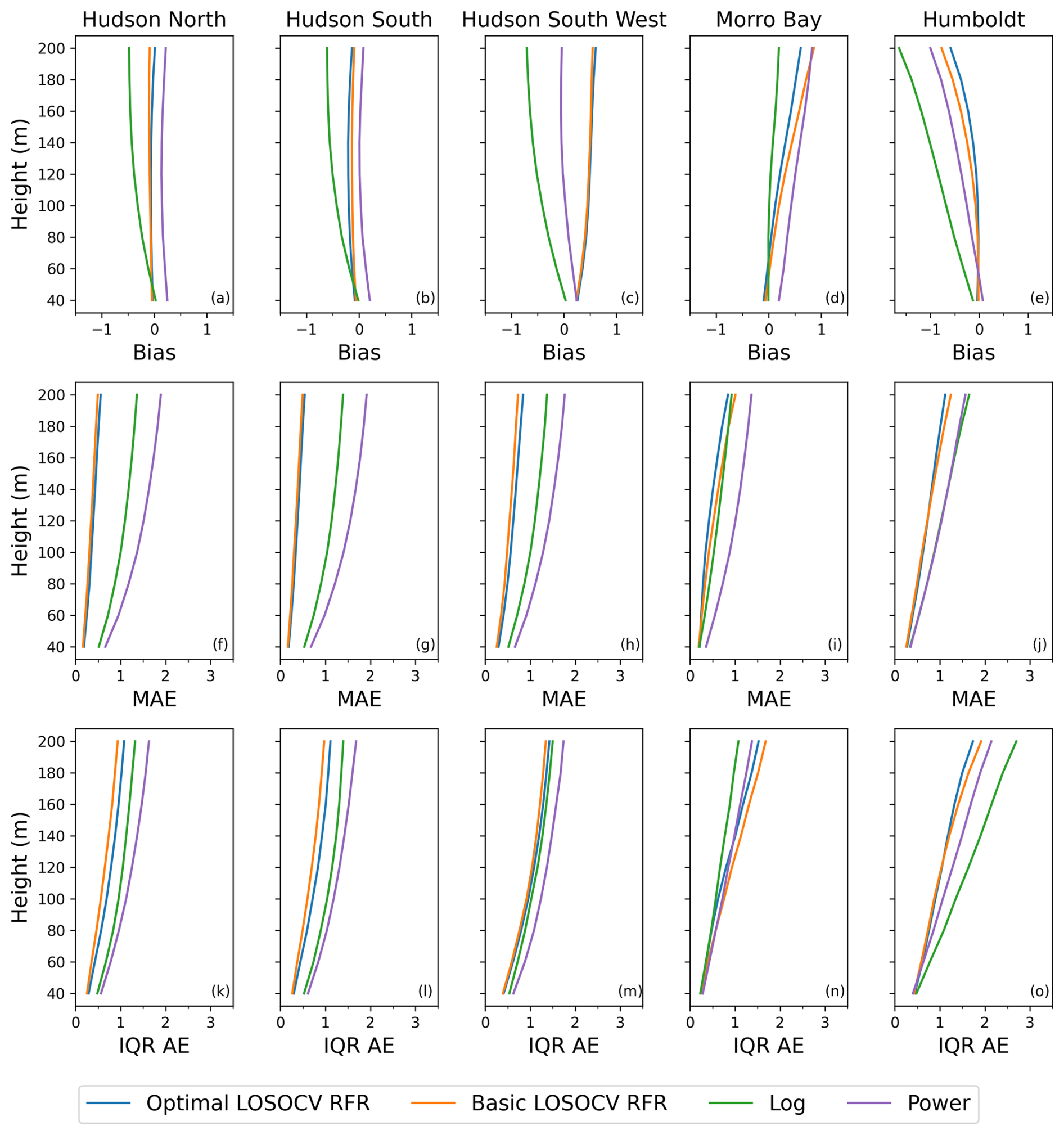
Figure 4 Bias (a–e), median absolute error (MAE; f–j), and interquartile range of the absolute error (IQR AE; k–o) profiles at each station for the optimal LOSOCV RFR, basic LOSOCV RFR, neutral log law, and power law. All plots have units of m s⁻¹.

For the majority of the lidar sites, the optimal LOSOCV RFR shows the smallest bias for all heights (Fig. 4a–e), especially at Hudson North and Hudson South, where there is negligible bias throughout all profiles, and at Humboldt, where all models increasingly underestimate the wind speeds with height. While the logarithmic law is the least biased at Morro Bay, the optimal LOSOCV RFR clearly outperforms the basic LOSOCV RFR and power law. The only station where the optimal LOSOCV RFR does not have an advantage in bias is Hudson South West, where it is comparable to the basic LOSOCV RFR with a positive bias and the log law with a negative bias of a similar magnitude and worse compared to the power law, which is mostly unbiased. Overall, the optimal LOSOCV shows lower biases on average more consistently than the other models, even if the log and power laws are both the least biased at one station each.

With respect to MAE, both RFRs consistently outperform both the log and the power laws, showing an overall increase in accuracy of the RFR compared to the conventional methods (Fig. 4f–j). The only exception is the log law at Morro Bay, which slightly outperforms the basic LOSOCV RFR at the top of the profile but falls short compared to both RFRs throughout the rest of the profiles. Comparing the two RFR models, the optimal LOSOCV RFR outperforms the basic LOSOCV RFR at both Morro Bay and Humboldt, and the basic LOSOCV performs marginally better at the three Hudson stations. Since the Hudson stations are in the same region, it is possible that other inputs in the basic LOSOCV RFR that are not present in the optimal LOSOCV RFR could potentially help capture some regional information, which could possibly explain the better performance at these stations compared to Humboldt and Morro Bay, where no regional information is included from other nearby stations in the LOSOCV model. Similar results are shown for the IQR AE (Fig. 4k–o) at all stations, with the exception of both conventional methods outperforming the RFRs at Morro Bay, showing that they have a lower spread in their differences than the RFRs at this station but a higher spread in differences at the other four stations. Overall, the RFR models show lower errors more consistently compared to the other methods. While the basic LOSOCV RFR may have marginally lower errors at the three Hudson stations, having lower errors at the Humboldt and Morro Bay stations, in addition to the lower number of inputs for our model, is worth the marginal decrease in accuracy at the Hudson stations.

5.2 High-shear events and low-level jets

As high-vertical-wind-shear events and LLJs both play important roles in wind energy production and load on wind farms (Borvarán, et al., 2020; Gadde and Stevens, 2021; Doosttalab et al., 2020), it is important to accurately model these phenomena. In this section, we evaluate the performance of the RFR in both LLJs and high-shear events and compare it with the performance of the conventional models. It is important to note that while LLJs can have a maximum anywhere within the first 1000 m, our training data only reach up to 200 m. Thus, only LLJs with a maximum below 200 m are identified in this analysis.

While the structures of these phenomena are known and can often be distinguished visually (Fig. 5), an exact rigorous physical criterion to identify these profiles is somewhat elusive. For the purpose of this study, they are defined in part following the definition used by Debnath et al. (2021), where the 90th percentile in vertical wind speed gradient ($\frac{\mathrm{d}u}{\mathrm{d}z}=$ 0.035 m s⁻¹ m⁻¹) was used as a threshold for high shear at the Hudson North and Hudson South buoys. While Debnath et al. (2021) considered the gradient only between heights within the rotor layer of a turbine (40–160 m), we consider all heights in our analysis as we are interested in model performance at all heights. For this analysis, LLJs are defined as profiles with a nose (height of wind gradient inversion) below 200 m, $\frac{\mathrm{d}u}{\mathrm{d}z}$ > 0.035 m s⁻¹ m⁻¹, where $\frac{\mathrm{d}u}{\mathrm{d}z}$ is the vertical wind speed gradient between 10 m and the nose, and a decrease in wind speed from the nose to the top of the profile that is greater than both 1.5 m s⁻¹ and 10 % of the maximum wind speed (Fig. 5f–j). A high-shear event is defined as a profile not already classified as an LLJ and where $\frac{\mathrm{d}u}{\mathrm{dz}}$ > 0.035 m s⁻¹ m⁻¹, with $\frac{\mathrm{d}u}{\mathrm{d}z}$ calculated as the gradient between 10 and 200 m (Fig. 5k–o). Any profiles that do not fit these criteria are grouped together as “normal” profiles for this analysis (Fig. 5a–e).

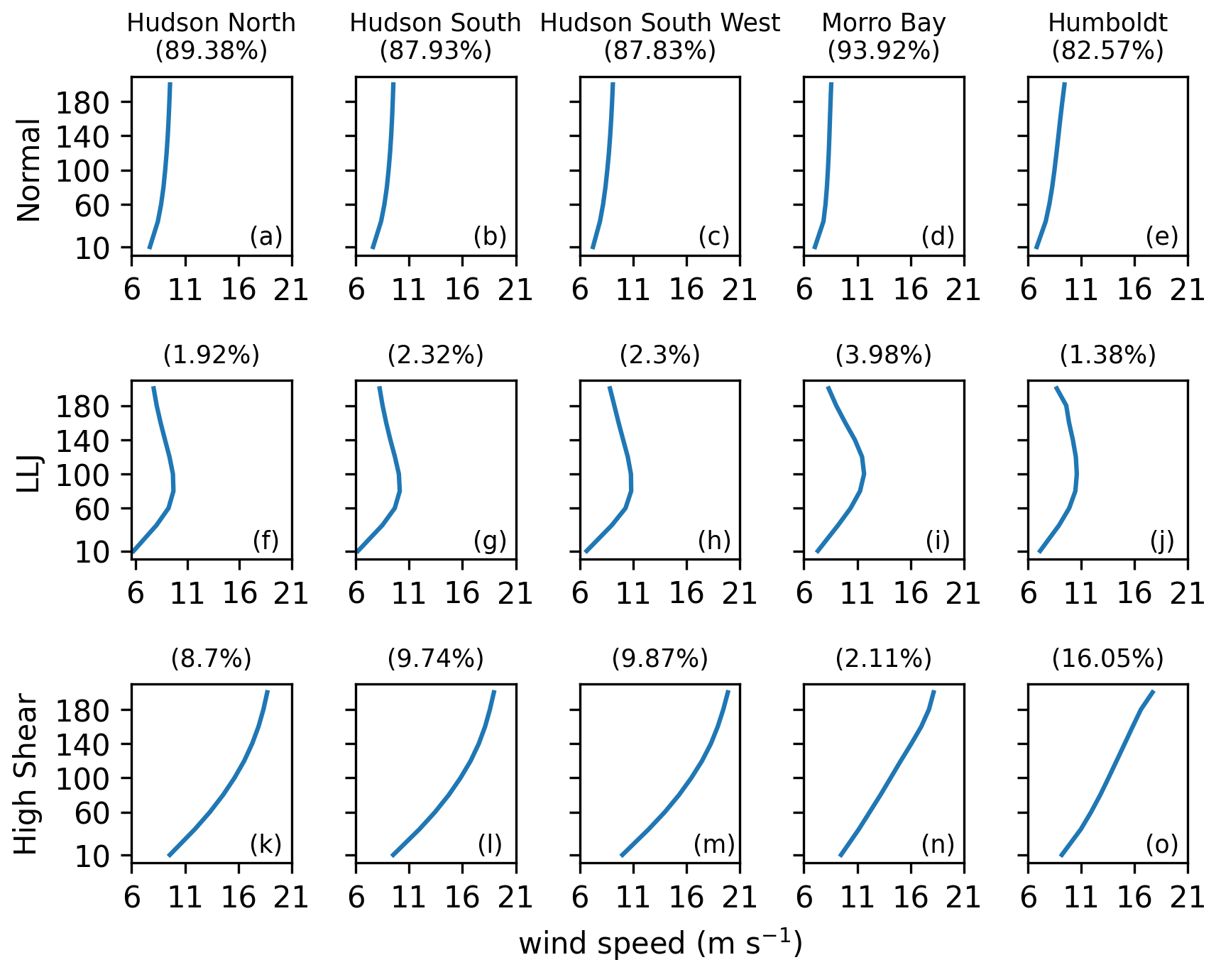
Figure 5 Mean wind speed profiles (m s⁻¹) for normal profiles (a–e), low-level jets (f–j), and high-shear events (k–o) at each station. Percentages correspond to the percent of total observations at each station in each group.

Though these LLJ and high-shear-event definitions may not capture every single profile of these phenomena, they capture the majority, and the model errors for each profile type will be representative. Normal profiles account for 82 %–94 % of the data at all training/validation stations; LLJs account for 1 %–4 % of the data at all training/validation stations; and high-wind-shear profiles account for 8 %–10 % of the data at the Hudson stations, 2 % of the data at Morro Bay, and 16 % of the data at Humboldt (Fig. 5). The previous error analysis was then repeated separately for each of the three profile types (Figs. 6–8).

Figure 6 Same as Fig. 4, except metrics are only for normal profiles.

Figure 7 Same as Fig. 4, except metrics are only for profiles with high-shear events.

Figure 8 Same as Fig. 4, except metrics are only for profiles with low-level jets.

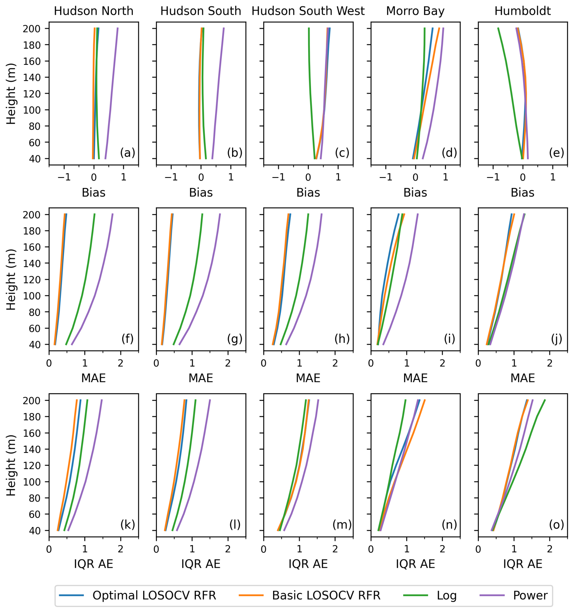
All models' performance on the normal profiles is relatively similar to the performance of the models on the full dataset, which is not surprising since the normal profiles comprise > 82 % of the data at each site (Fig. 6). For normal profiles, both RFRs still generally outperform the other methods at all stations and heights. Only at Humboldt is the optimal RFR bias less for the normal profiles than for all the profiles combined.

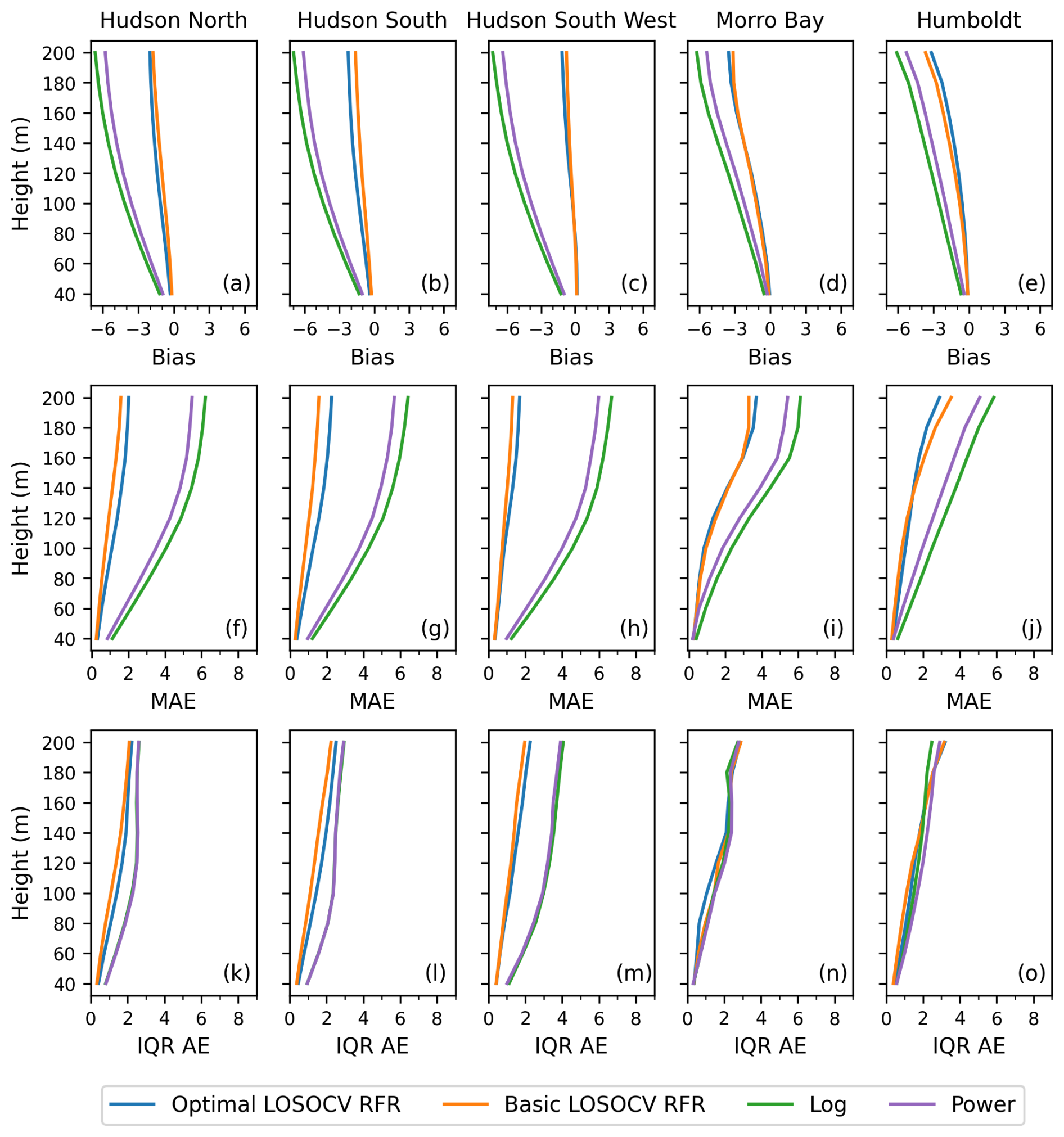
For high-shear events, both RFRs vastly outperform the neutral log and power laws (Fig. 7). While all models show increasingly negative biases through the profile and underestimate the high-shear events, the log and power laws do not capture the high-shear events at all, whereas the RFRs can capture them but underestimate them on average. Similar to bias, the RFRs have much lower MAEs than the conventional methods, showing their strength in predicting high-shear events. The same holds true for the IQR AEs at the Hudson stations. However, the RFRs show a similar spread in absolute errors at Morro Bay and Humboldt compared with the conventional methods. The basic LOSOCV RFR shows slightly better performance in high-shear events at every station other than Humboldt, which shows that the features excluded from the optimal RFR may help with capturing high-shear events. Since we are interested in the highest performance overall and the optimal LOSOCV RFR shows the best performance overall, we still prefer it over the basic LOSOCV RFR. However, if a model needed for the purposes of high-shear events specifically was created, it would warrant considering additional features.

For profiles with LLJs, the RFRs generally outperform the other methods below and up to wind turbine hub heights but perform worse above (Fig. 8). The RFRs appear to capture the initial high shear in the profile; however they fail to predict the decrease in wind speeds above the inversion. This can be seen in the biases of the RFRs at each station, which are relatively small at lower heights but greatly increase at the tops of the profiles, and in their MAEs, where the errors are low up to turbine hub heights and increase above. Neither the log law nor the power law captures the initial high shear of LLJs, but they both predict more accurately at the top of the profiles than the RFRs. As such, the RFR models are preferred for computing wind speeds at hub heights but may still fall short in energy assessment for LLJs with an inversion layer below 200 m, since determining rotor-equivalent wind speeds requires accurate measurements at all heights within the rotor layer of a turbine. Similar to high-shear events, the basic RFR seems to outperform the optimal RFR slightly on profiles with LLJs, which suggests that training a separate RFR with additional features could improve the model's accuracy at capturing the full structure of the LLJ profiles.

Investigating the distribution of w₁₀ and ΔT values for each group of profiles (normal, LLJ, high shear) shows the model's capability to accurately reproduce normal and high-wind-shear profiles but only the lower part of the LLJ profiles. After running the w₁₀ and ΔT values from the training data back through the final optimal RF, we can use the definitions above to classify the predicted profiles and compare those group assignments to those of the observed full profiles across the feature space (Fig. 9). Many high-shear events have a combination of high w₁₀ and strongly positive ΔT that is never observed in normal and LLJ profiles. As such, it is encouraging that the RFR model always produces a high-shear profile when fed a sufficiently large w₁₀ (> ∼ 7 m s⁻¹) and positive ΔT (> ∼ 1 °C). Observed LLJ and high-shear profiles rarely have ΔT < −1 °C, so it is also encouraging that all profiles produced by the RFR using ΔT values in this range were normal profiles. However, there is no clear region in the feature space for the model to always predict an LLJ, as the LLJ region of the feature space always coincides with that of the normal and/or high-shear groups. This, combined with the relatively low number of LLJ observations compared to normal and high-shear profiles, may explain why the RFR does not correctly predict LLJs, as the model cannot differentiate them from other profiles with only the given features. For the inversion in an LLJ to be captured, a more complex model and/or other inputs are needed.

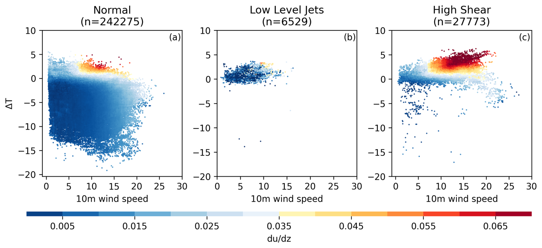
Figure 9 Air–sea temperature difference (ΔT, °C) and 10 m wind speed (w₁₀, m s⁻¹) for (a) normal, (b) low-level jet, and (c) high-shear profiles, grouped based on the observed profiles. Wind speed gradients ($\frac{\mathrm{d}u}{\mathrm{d}z})$ based on the RFR estimate of each profile are shown. The gradient for normal and high-shear profiles is calculated between the surface and the top of the profiles, while the gradient for LLJs is calculated between the surface and the height of the maximum wind speed.

6 Extrapolation model performance on test data

6.1 Comparison with independent lidar station data

The ASOW-4 and ASOW-6 lidar stations were not used during the training and validation of the optimal RFR model and can therefore be used as a completely independent test dataset to assess the ability of the model (specifically the final version trained on all five training/validation sites) to perform on unseen data (i.e., to “generalize”) and to generate initial uncertainties on the RFR-based estimates. The ASOW stations are of particular interest as they contain higher percentages of LLJs and high-shear events than any of the training/validation stations (except Humboldt): 5.70 % (LLJ) and 14.54 % (high shear) at ASOW-4 and 4.43 % (LLJ) and 15.58 % (high shear) at ASOW-6. A total of 16.05 % of profiles at Humboldt were classified as high shear. Together, the LLJ and high-shear profiles account for ∼ 20 % of the data at the ASOW stations, showing that accurately predicting these profiles is important for robust resource assessment at certain locations. The w₁₀ and ΔT values from all profiles at both stations are separately extrapolated to full wind profiles from 40–200 m by the power law, neutral log law, and optimal RFR models and then compared to the observed profiles. The performance of the RFR at stations ASOW-4 and ASOW-6 is comparable to the performance at the five training/validation stations, suggesting the model can perform similarly well at locations it was not trained on (Figs. 10 and 11).

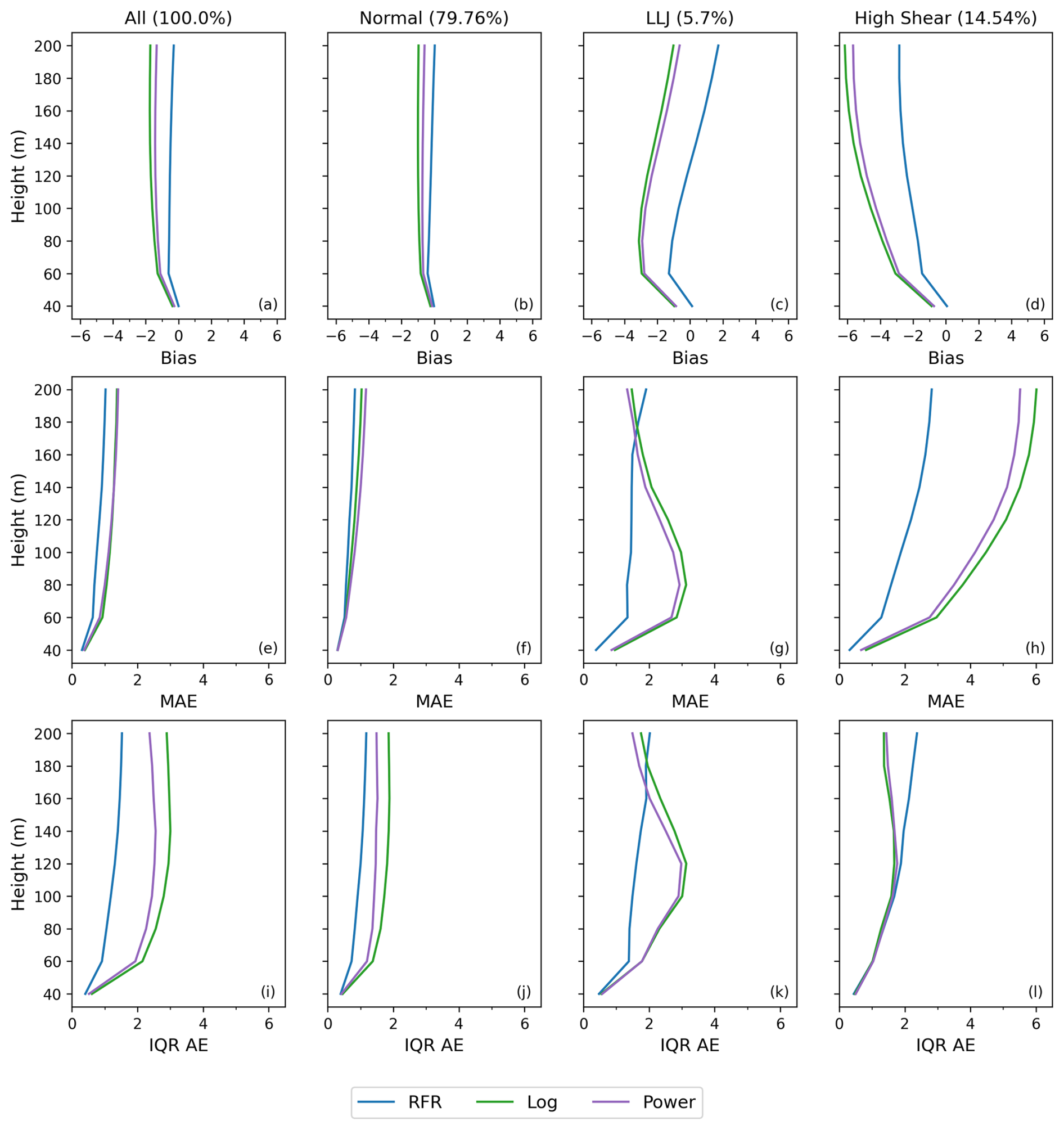
Figure 10 Bias (a–d), median absolute error (MAE; e–h), and interquartile range of the absolute error (IQR AE; i–l) profiles at the ASOW-4 station for the optimal RFR, neutral log law, and power law models. All plots have units of m s⁻¹.

Figure 11 Same as Fig. 10 but for the ASOW-6 station.

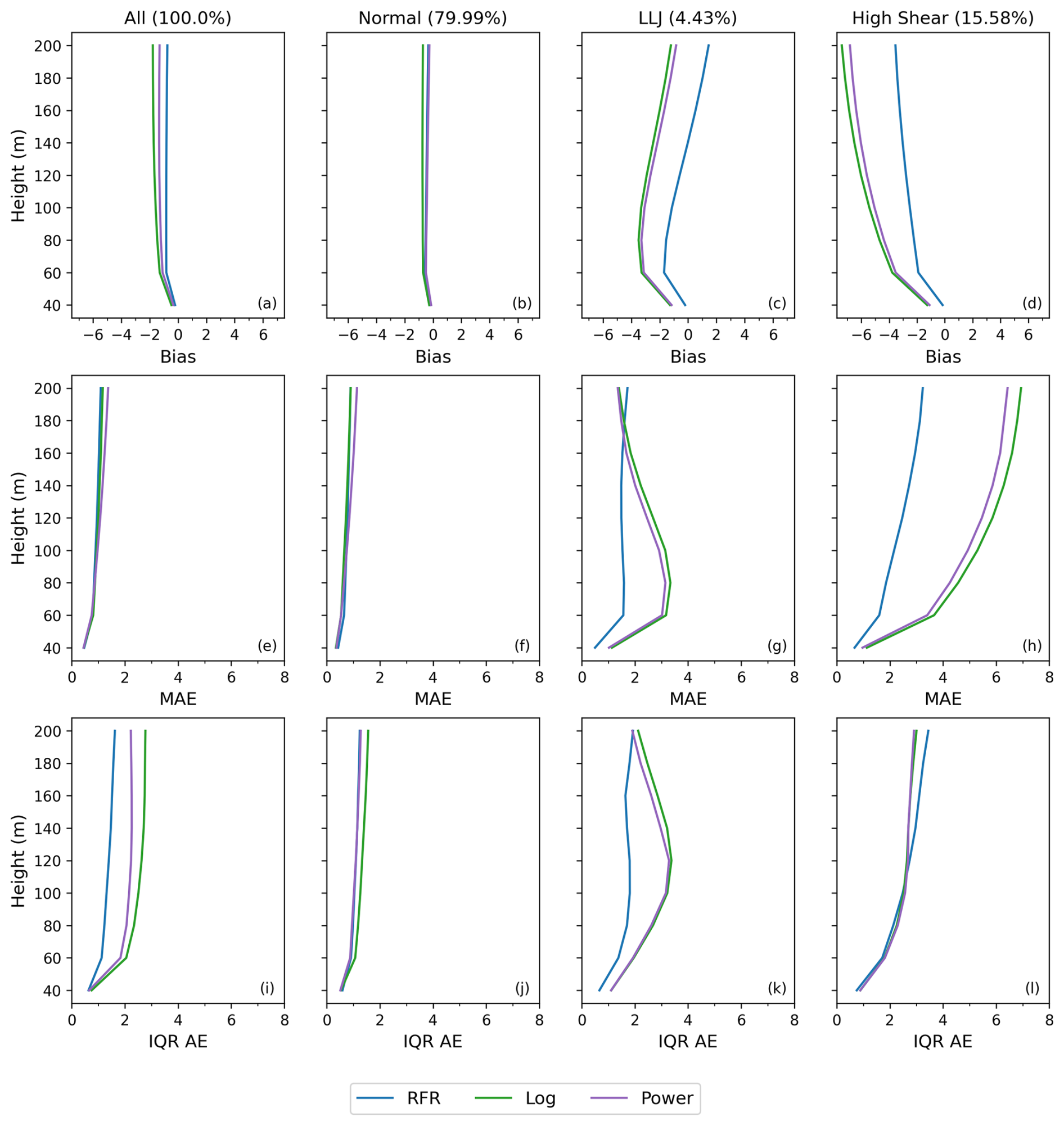
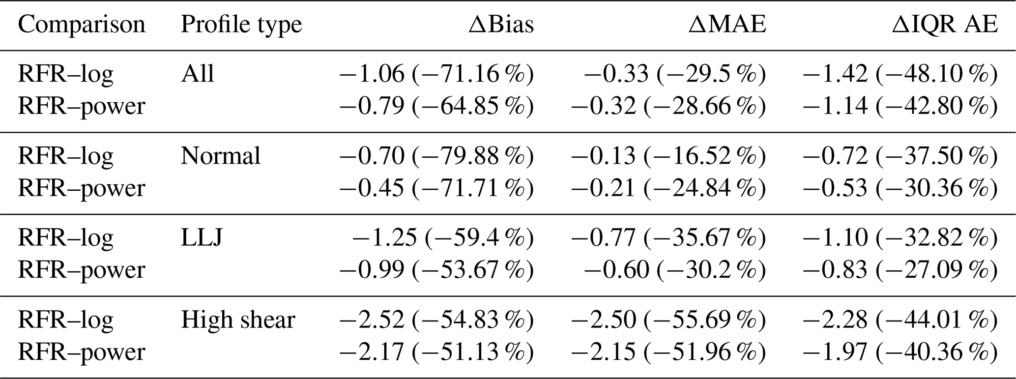
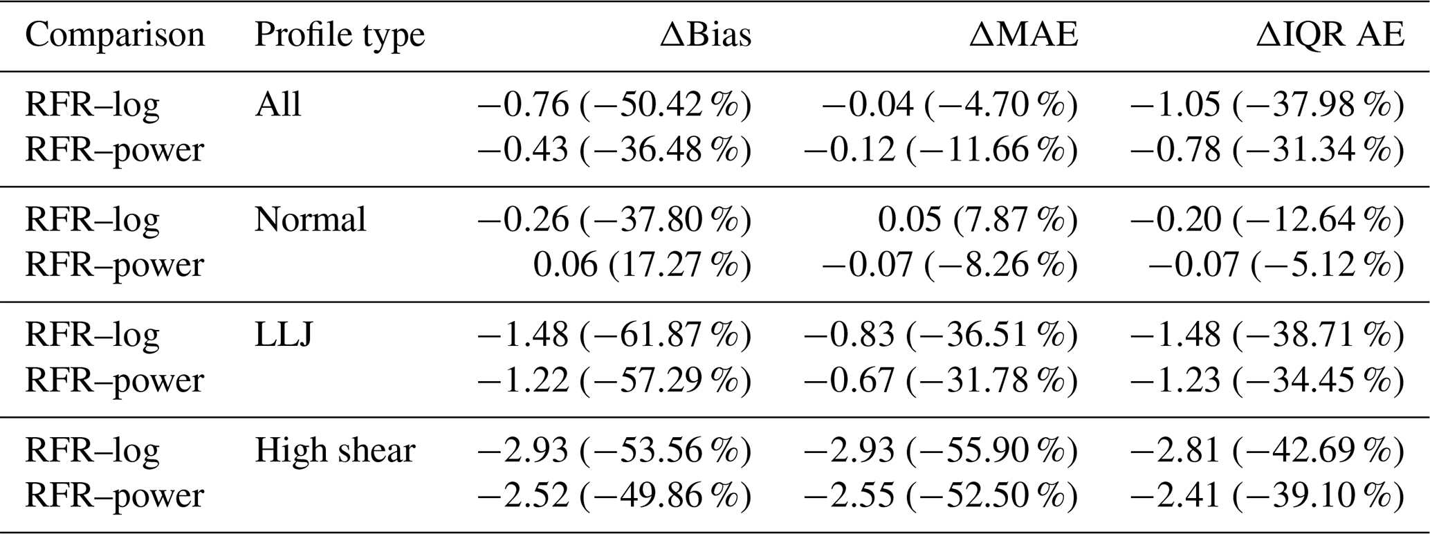
At both ASOW-4 and ASOW-6, the RFR shows considerable improvement over both the neutral log and the power laws. For ASOW-4, the RFR outperforms the other models at all heights for every profile type, except for having larger errors at 180 and 200 m for LLJs where the RFR failed to capture the wind speed gradient inversion (Table 2, Fig. 10), consistent with the above analysis on the training/validation stations. At ASOW-6, the RFR still outperforms the conventional methods overall but is shown to have a bias comparable to the power law and an MAE comparable to the neutral log law for normal profiles, in addition to the higher errors at 180 and 200 m for LLJ profiles (Table 3, Fig. 11). However, this is not due to a decline in the RFR's performance. Instead, the bias and MAE of the RFR for normal profiles at ASOW-6 are comparable to those of the conventional methods as the other methods have increased accuracy at this station compared to at ASOW-4. As such, even when the neutral log and power laws skillfully predict at the given stations, they are still only comparable to the RFR and do not ever substantially outperform the RFR, except for at the highest heights of the LLJ profiles. In addition, the conventional methods never once achieve performance comparable to that of the RFR on high-shear profiles or up to the turbine hub heights of LLJ profiles. This shows that the RFR still has increased performance overall compared to conventional methods at locations independent of training and validation. The error metrics at these two independent test stations also provide initial estimates of the uncertainty on the RFR-based estimates at other locations independent of training and validation.

Table 2 Average change in bias, MAE, and IQR AE for the optimal RFR compared to conventional methods for different profile types at ASOW-4. Units are in m s⁻¹.

Table 3 Same as Table 2 but for ASOW-6.

6.2 Comparison with NREL profiles

NREL NOW-23 wind speed profiles from 2019 at six offshore locations around US coasts are used to further assess how well the RFR model can perform at stations that it was not trained on (locations provided in Fig. 12). These stations are representative of a number of different important oceanic regions around the coastal US. For this comparison, the RFR-estimated profiles are generated using w₁₀ and ΔT from the NOW-23 dataset. This will allow us to directly compare our RFR-estimated wind profiles with NOW-23's WRF-based output to evaluate differences between the extrapolation methods.

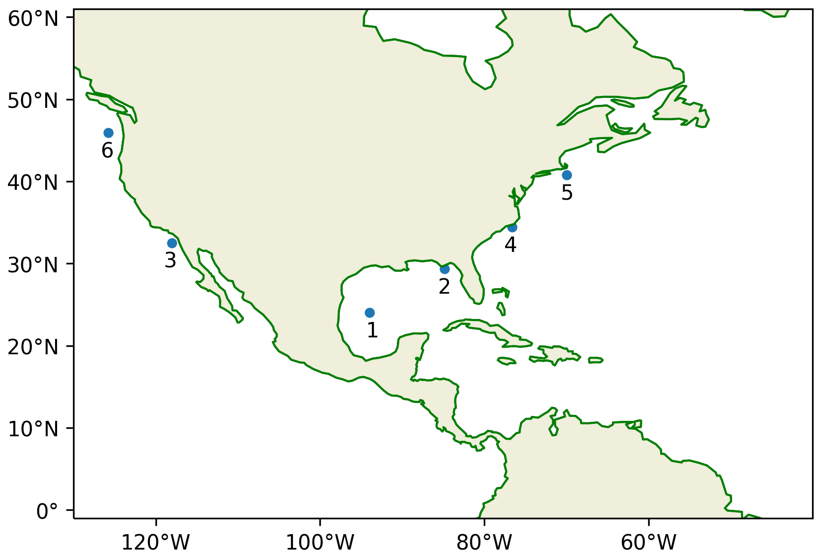
Figure 12 Locations of the six NREL stations used for independent testing of the RFR model.

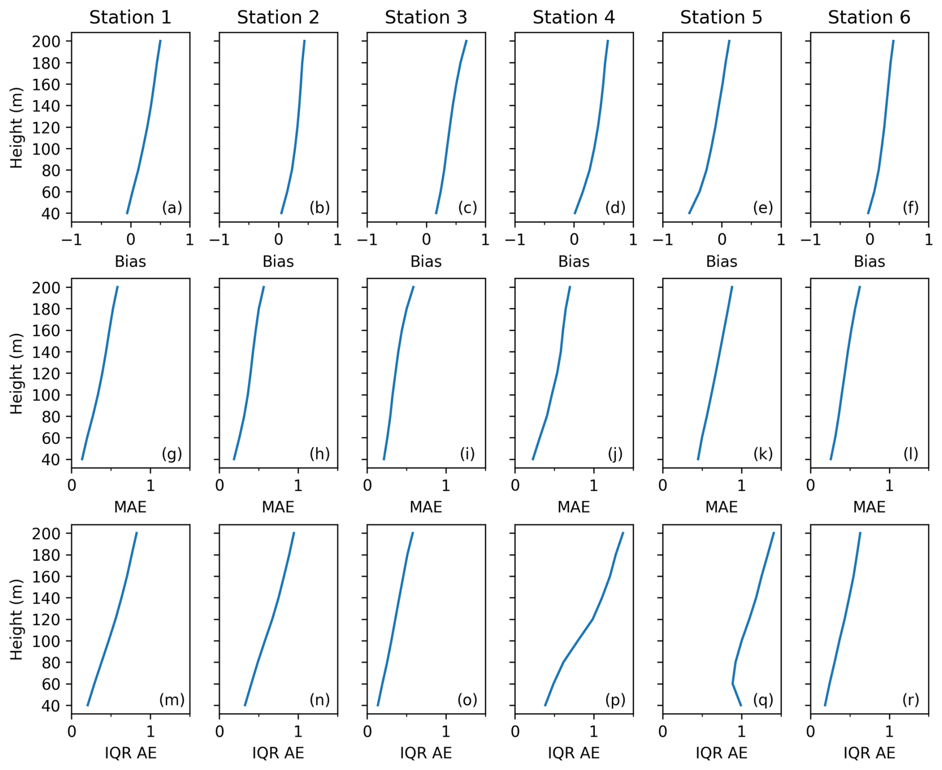
Figure 13 Bias (a–f), median absolute error (MAE; g–l), and interquartile range of the absolute error (IQR AE; m–r) profiles at each of the six NOW-23 stations for the profiles extrapolated by the RFR vs. the observed profiles from NOW-23. All plots have units of m s⁻¹.

To assess the performance of the RFR at these stations, the full profiles from the NOW-23 dataset are used as the “observed” profiles for the error analysis. For most of the stations, the consistent positive bias demonstrates that the RFR consistently overestimates wind speed at all heights, relative to the NOW-23 profiles (Fig. 13a–f). At station 5 the RFR underestimates wind speeds from the ground to 140 m and then increasingly overestimates wind speeds from 140 to 200 m. This bias throughout the profile remains within ±1 m s⁻¹. The MAEs never exceed 1 m s⁻¹ (Fig. 13g–l) and IQR AEs never exceed 1.5 m s⁻¹ (Fig. 13 m–r) at any station. Overall, when the RFR model uses w₁₀ and ΔT values from NOW-23 to predict wind speed profiles at six different offshore locations than where the model training data were collected, it does not greatly affect the model's accuracy, and the statistics are similar to those previously seen with lidar station comparisons (Figs. 4, 10, and 11). This shows that our model can perform skillfully around the coasts of the contiguous US, including regions not included in the training data, such as the Gulf of Mexico, Pacific Northwest, and central East Coast. To our knowledge, no previous studies have shown that an RFR model can successfully extrapolate wind speeds at locations this far from the training data.

7 Application of RFR to NBSv2.0 and uncertainty quantification

Once the final optimal RFR has been trained, validated, and tested, we apply this model to the NBSv2.0 w₁₀ data and ERA5 ΔT values at 6-hourly resolution from 1987 to the present with near-real-time updates (1 d latency) to generate a long-term wind speed profile product from 20 to 200 m (as well as the surface value at 10 m) on a 0.25° grid named NOAAOffshoreWindProfiles-USA. As the RFR only provides estimates between 40 and 200 m, these profiles are extended down to 20 m using the power law to interpolate between the 10 m (from NBSv2.0) and 40 m (from NOAAOffshoreWindProfiles-USA) wind speeds. NOAAOffshoreWindProfiles-USA will be archived with NCEI for public access. Seasonal climatological wind speeds are calculated from the NOAAOffshoreWindProfiles-USA 6-hourly data at three heights (20, 100, and 200 m) to highlight some of the variability that can be resolved with this product (Fig. 14). Long-term mean wind speeds are the highest over the subpolar North Atlantic and North Pacific oceans in all seasons and at all heights, with wind speeds increasing with height over these regions. While the wind speeds over most of the domain show a decrease in the boreal summer, winds over the California Current System (CCS) are stronger in these months (consistent with Huyer, 1983), especially at 100 and 200 m. Other than in the CCS region, wind speeds at turbine hub heights over our domain of interest reach a maximum in boreal winter.

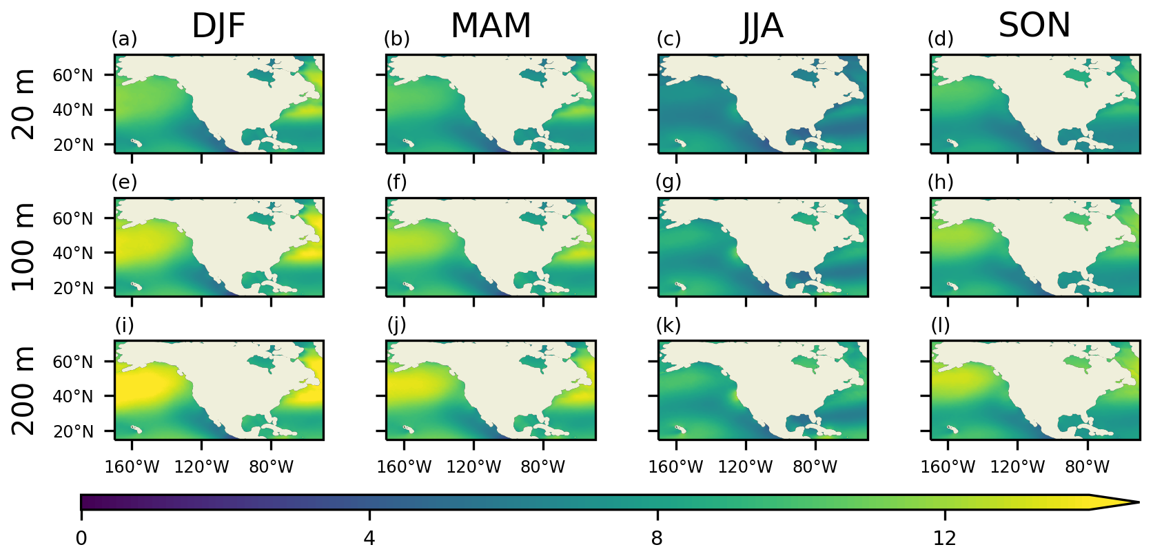
Figure 14 The 1987–2022 seasonal climatologies for wind profiles extrapolated from NOAAOffshoreWindProfiles-USA (m s⁻¹) at 20 (a–d), 100 (e–h), and 200 m (i–l). DJF – December, January, February. MAM – March, April, May. JJA – June, July, August. SON – September, October, November.

The inherent problem in trying to estimate the uncertainties in the NOAAOffshoreWindProfiles-USA wind profiles by using the NOW-23 profiles is that although the NOW-23 profiles can be regarded as “reference” or “true” values for the comparison, they still have errors as well. Therefore, any statistics for the NOAAOffshoreWindProfiles-USA profiles will need to be relative to how many errors are in the reference profiles. The error in the NOW-23 profiles can originate from many sources, including the NWP model (WRF) uncertainties/errors related to the boundary conditions, parametric uncertainty in the model, and errors in input parameters that are included in the WRF model. Bodini et al. (2024) quantify this uncertainty in the NWP model in terms of bias, centered RMSE, standard deviation, and correlation coefficient with respect to both independent lidar and National Data Buoy Center buoy data.

To estimate the error in our product despite these issues, the triple-collocation (TC) method is employed. In the TC error analysis, three or more mutually independent datasets can be used to estimate the RMSEs (relative to the unknown “ground truth”) of each dataset with good accuracy (McColl et al., 2014; Saha et al., 2020). The basic assumption in this three-way analysis is that it considers a linear error mode given by Eq. (5), where X_i values (with i= 1, 2, 3) are collocated measurement systems linearly related to the true value of t, with ε_i as additive random errors and α_i and β_i as the ordinary least-squares intercept and slope, respectively. We estimate the RMSE of ε_i denoted by ${\mathit{\sigma }}_{{\mathit{\epsilon }}_i}$.

$$\begin{array}{}\text{(5)}& X_i={\mathit{\alpha }}_{i}t+{\mathit{\beta }}_i+{\mathit{\epsilon }}_i\end{array}$$

Another assumption is that all three datasets are mutually uncorrelated ($<{\mathit{\epsilon }}_i{\mathit{\epsilon }}_j>=\mathrm{0})$ and that they are also uncorrelated with the true value, t ($<t{\mathit{\epsilon }}_i>=\mathrm{0})$. McColl et al. (2014) provide an extended triple-collocation (ETC) method to estimate the RMSEs for all data along with their sensitivities to the true wind speeds. In the case of three datasets with independent errors, the RMSEs can be derived using Eq. (6) (Saha et al., 2020), where σ_ε is the RMSE, and each Q represents the variance between the two datasets indicated in the subscript:

$$\begin{array}{}\text{(6)}& {\mathit{\sigma }}_{\mathit{\epsilon }}=\left[\begin{array}{l}\sqrt{Q_{\mathrm{11}}-\frac{Q_{\mathrm{12}}{Q}_{\mathrm{13}}}{Q_{\mathrm{23}}}}\\ \sqrt{Q_{\mathrm{22}}-\frac{Q_{\mathrm{12}}{Q}_{\mathrm{23}}}{Q_{\mathrm{13}}}}\\ \sqrt{Q_{\mathrm{33}}-\frac{Q_{\mathrm{13}}{Q}_{\mathrm{23}}}{Q_{\mathrm{12}}}}\end{array}\right].\end{array}$$

Given the interest in the wind energy sector and the limited availability of independent wind profile datasets, we do this ETC analysis at 100 m only. The three datasets used for this analysis are NOAAOffshoreWindProfiles-USA, NOW-23, and ERA5 from 2015 to 2019 at 6-hourly resolution, with NOW-23 averaged into 6-hourly observations from its original 5 min data. As NOW-23 uses ERA5 as input, the assumption of independence breaks down between these two datasets, resulting in unrealistic, negative variances in Eq. (5) (see Appendix A for more details). Therefore, we employ the modified version of ETC provided in González-Gambau et al. (2020), the correlated triple collocation (CTC), which allows for two out of the three datasets to be error correlated. CTC assumes that the errors between datasets 1 and 2 are correlated, with covariance $<{\mathit{\epsilon }}_{\mathrm{1}}{\mathit{\epsilon }}_{\mathrm{2}}>\ne \mathrm{0}$; however they are completely uncorrelated with the error in the third dataset, i.e., $<{\mathit{\epsilon }}_{\mathrm{1}}{\mathit{\epsilon }}_{\mathrm{3}}>=\mathrm{0}$ and $<{\mathit{\epsilon }}_{\mathrm{2}}{\mathit{\epsilon }}_{\mathrm{3}}>=\mathrm{0}$. For such cases using CTC, RMSEs are given by

$$\begin{array}{}\text{(7)}& {\mathit{\sigma }}_{\mathit{\epsilon }}=\left[\begin{array}{l}\sqrt{v^{\mathrm{2}}{Q}_{\mathrm{11}}^{\prime }+Q_{\mathrm{22}}^{\prime }-Q_{\mathrm{23}}^{\prime }}\\ \sqrt{u^{\mathrm{2}}{Q}_{\mathrm{11}}^{\prime }+Q_{\mathrm{22}}^{\prime }-Q_{\mathrm{23}}^{\prime }}\\ \sqrt{Q_{\mathrm{33}}-Q_{\mathrm{23}}^{\prime }}\end{array}\right],\end{array}$$

where u and v can be expressed in terms of the variances as $u=\frac{Q_{\mathrm{22}}-Q_{\mathrm{12}}}{Q_{\mathrm{11}}+Q_{\mathrm{22}}-\mathrm{2}{Q}_{\mathrm{12}}}$ and $v=\frac{Q_{\mathrm{11}}-Q_{\mathrm{12}}}{Q_{\mathrm{11}}+Q_{\mathrm{22}}-\mathrm{2}{Q}_{\mathrm{12}}}$, with $Q_{\mathrm{11}}^{\prime }=Q_{\mathrm{11}}+Q_{\mathrm{22}}-\mathrm{2}{Q}_{\mathrm{12}}$, $Q_{\mathrm{22}}^{\prime }=u^{\mathrm{2}}{Q}_{\mathrm{11}}+v^{\mathrm{2}}{Q}_{\mathrm{22}}+\mathrm{2}uv{Q}_{\mathrm{12}}$, and $Q_{\mathrm{23}}^{\prime }=u{Q}_{\mathrm{12}}+v{Q}_{\mathrm{23}}$. For a detailed derivation, refer to Appendix A3 of González-Gambau et al. (2020).

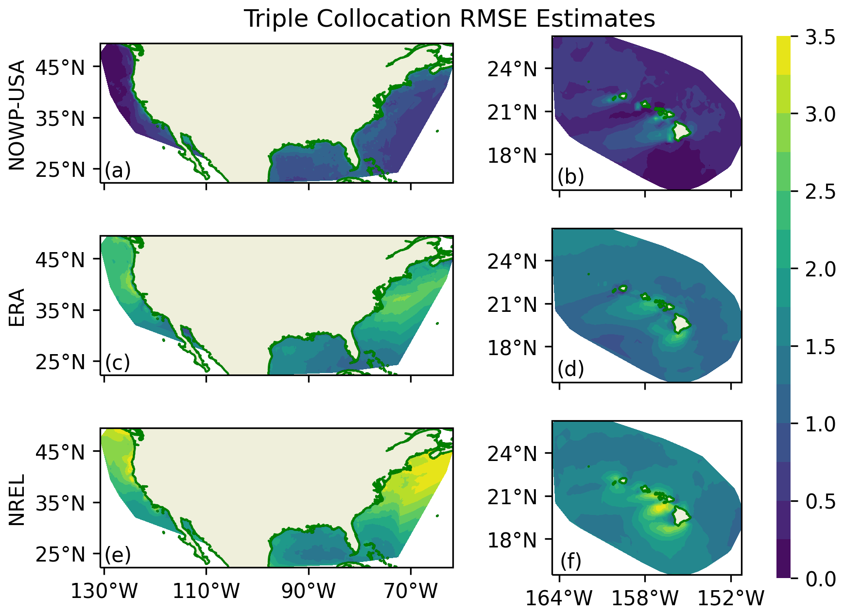
Figure 15 Correlated triple-collocation RMSE estimates (m s⁻¹) around the coastal regions of the contiguous US and Hawai`i for the NOAAOffshoreWindProfiles-USA (NOWP-USA) (a–b), ERA5 (c–d), and NOW-23 datasets (e–f).

Using the CTC formulation, the RMSEs are estimated at each grid point where all three datasets were collocated around the contiguous US and Hawai`i (Fig. 15). The number of triple collocations (matchups) that are used to estimate these RMSEs is ∼ 56 million, which corresponds to 5 years of collocated data between the three products. RMSEs are the lowest for NOAAOffshoreWindProfiles-USA (∼ 0.01–2 m s<sup>−1</sup>), followed by ERA5 (∼ 0.17–3.5 m s<sup>−1</sup>) and then NOW-23 (∼ 0.65–4.2 m s<sup>−1</sup>). These RMSEs for NOAAOffshoreWindProfiles-USA are comparable to the RMSEs calculated above at the two test lidar stations (1.4–1.8 m s<sup>−1</sup>), indicating that the error metrics at those stations were a reasonable estimation of the RFR's ability to generalize to unseen data. All three products have particularly high RMSEs southwest of Hawai`i, coinciding with the unique wind wake found in this region (Xie et al., 2001).

We divided the analysis region further into seven coastal regions of interest for the offshore wind energy sector and calculated regional-scale RMSEs using the matchups in each region. These seven regions are the North Atlantic coast (NAC), mid-Atlantic coast (MAC), South Atlantic coast (SAC), Pacific Northwest (PNW), Gulf of Mexico (GoM), offshore California (OC), and Hawaiian coast (HC) (see Fig. 1 in Bodini et al., 2024). The number of matchups between the three datasets at 100 m varies substantially around the coasts of the contiguous US and Hawai`i (from ∼ 4 to ∼ 13 million; Table 4) due to the varying size of each region. In all seven regions, NOAAOffshoreWindProfiles-USA has lower RMSEs (∼ 0.2–1.1 m s⁻¹) than the other products (∼ 1.5–3.5 m s⁻¹ for both the ERA5 and the NOW-23 data) (Table 4).

Table 4 RMSEs for all three products (NOAAOffshoreWindProfiles-USA, ERA5, and NOW-23) and number of triple matchups at 100 m for the seven different regions (North Atlantic coast (NAC), mid-Atlantic coast (MAC), South Atlantic coast (SAC), Pacific Northwest (PNW), Gulf of Mexico (GoM), Californian coast (OC), and Hawaiian coast (HC)) in the coastal US. All RMSEs are in m s⁻¹.

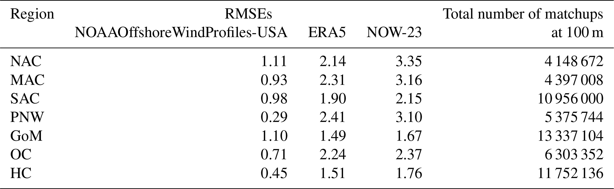
Bodini et al. (2024) use a comprehensive approach of comparing the 20 years of NOW-23 wind speed data at 140 m with winds extrapolated using a machine-learning-based model output and report an uncertainty of below 3 m s⁻¹ across the considered regions. However, the current analysis shows that in regions like the NAC, MAC, and PNW at 100 m, the uncertainties in NOW-23 wind speeds exceed 3 m s⁻¹, and it is plausible that the RMSEs could be even higher for higher hub heights.

8 Conclusions

Conventional methods for wind speed profile extrapolation, such as the logarithmic and power laws, have limitations and greatly underestimate wind power production in many applications. As such, there is a need for new methods of wind speed extrapolation, which has led to the use of machine learning for this problem in the past decade. This study focused on building a machine learning model (RFR) to predict wind speed profiles (from 40 to 200 m above the ocean's surface) around the coastal regions of the contiguous US and Hawai`i using a gridded satellite-based surface wind speed product (NBSv2.0) as input. This study shows that the RFR algorithm outperforms and is more consistent than the logarithmic and power laws at five lidar stations off the coasts of New York and California when validating using LOSOCV. In addition, the final RFR model requires fewer input variables (w₁₀ and ΔT) than the other methods to predict vertical wind profiles. The RFR model outperforms traditional methods in particular when extrapolating the wind speeds at wind turbine hub heights under conditions of high vertical shear and LLJs. The only condition where the RFR model did not perform well was above the peak of LLJs, as it fails to predict the wind speed gradient inversions that take place there.

Independent testing of the RFR model using two additional lidar buoys confirms the RFR model's high performance at locations independent of the model's training and its ability to accurately predict profiles with high wind shear. While conventional methods can sometimes approach the accuracy of the RFR for normal profiles, their performance is much less consistent and never significantly better than the RFR across all of the error metrics. In addition, the ability of the RFR to accurately predict high wind shear makes the model much more useful for wind energy applications than the conventional methods that fail to replicate the high shear. Further independent comparison against profiles from NOW-23 demonstrated the robustness of the RFR as the accuracy of the model does not deteriorate when it is used to extrapolate wind speeds at locations far from the training sites in New York and California, with errors at the various testing locations (off the Gulf of Mexico, East Coast, Washington State coast, and southern Californian coast) resembling those of the training sites.

Since the training, validation, and testing demonstrated that the RFR model can robustly predict wind speeds for the offshore regions of the contiguous US and Hawai`i, it could then be confidently applied to NBSv2.0 6-hourly 0.25° gridded data to produce 40 to 200 m wind profiles at this resolution (known as NOAAOffshoreWindProfiles-USA). These profile estimates were then extended down to 20 m by applying the power law model between the 10 m (from NBSv2.0) and 40 m (from NOAAOffshoreWindProfiles-USA) wind speeds. To assess the uncertainties in this product, a correlated triple-collocation analysis was performed using the NOAAOffshoreWindProfiles-USA, ERA5, and NOW-23 outputs at 100 m to estimate errors associated with each dataset relative to an unknown ground truth. Across the entire region tested, NOAAOffshoreWindProfiles-USA consistently had the smallest estimated errors. These results show the advantages of both using satellite-based data over reanalysis and implementing machine learning versus NWP models for this application.

We have demonstrated that the RFR model can robustly predict wind speeds during most conditions found over the coastal regions of the contiguous US and Hawai`i, and future work will continue to improve this model. This includes investigating the use of machine learning for wind extrapolation over larger regions and potentially exploring the use of more complex models. In addition, our RFR model currently lacks the capacity to predict the wind speed gradient inversion of an LLJ, so further research could include identifying other input variables that would be better able to predict these features in an LLJ wind speed profile. Despite these limitations, the RFR model introduced here greatly improves upon the conventional methods for extrapolating wind profiles, particularly over large regions simultaneously, and allows us to robustly produce a wind speed profile product over the coastlines of the contiguous US and Hawai`i.

Appendix A: Correlation between the three products

To estimate the error in our product, the triple-collocation (TC) method is employed. Initial implementation of Eq. (5) resulted in negative variances, which suggested at least two of the datasets were actually correlated, thereby disregarding one of the key assumptions of the ETC method. To identify which datasets were correlated, three bivariate density (i.e., joint probability) plots in their residual space are generated, where two products are compared each time, while the third dataset acts as an anchor (common difference) at all of the matchup locations (Fig. A1). With NOW-23 data as the anchor, the R² between ERA5 and NOAAOffshoreWindProfiles-USA is ∼ 0.006, while with ERA5 as the anchor, the R² between NOAAOffshoreWindProfiles-USA and NOW-23 is ∼ 0.113. When NOAAOffshoreWindProfiles-USA is the anchor, ERA5 and NOW-23 show a very high correlation (R²≈ 0.62, Pearson correlation coefficient value of ∼ 0.8, and p value of 0.0). Therefore, it is evident that NOAAOffshoreWindProfiles-USA is independent of the other two datasets, despite using T from ERA5 as one of the inputs. On the other hand, ERA5 and NOW-23 are highly correlated. This is likely because the WRF model used to develop the NOW-23 product is initialized and forced at the boundaries with ERA5 data (Rybchuk et al., 2021; Draxl et al., 2015a, b).

Figure A1 Comparisons in the residual space between (a) ERA5 and NOAAOffshoreWindProfiles-USA, (b) NOAAOffshoreWindProfiles-USA and NOW-23, and (c) ERA5 and NOW-23, where the third dataset in each case is used as an anchor (i.e., common difference) for the two datasets being compared (all in m s⁻¹). Each 0.5×0.5 m s⁻¹ bin is colored by the number of matchups in that bin. The solid line represents the linear regression fit, and the dashed line is the 1:1 line.