Integer programming for optimal yaw control of wind farms

It is well-known that wakes caused by wind turbines within a wind farm negatively impact the power generation and mechanical load of downstream turbines. This is already partially considered in the farm layout. Nevertheless, the strong interactions between individual turbines provide further opportunities to mitigate adverse effects during operation, e.g., by repeatedly adjusting axial induction or yaw offsets to wind conditions. We propose a mathematical approach that covers the farm by patterns based on a smaller, precomputable so-called upstream section, in the form of integer programming for faster globally optimal farm-level yaw control (under some mild assumptions, such as discretized yaw offsets, chosen size of the upstream section, and homogeneous layout structure). While we prove the wind farm yaw problem to be strongly 𝒩𝒫 hard in general, we demonstrate through numerical experiments that our method enables optimal farm-level yaw control under real-world control update periods. In particular, the approach remains efficient if turbines are deactivated, and it scales well with farm width.

1 Introduction

Wind turbines are considered one of the most important electric power plants of the future energy grid, since they can generate electricity cheaply and with low greenhouse gas emissions; see, e.g., Kost et al. (2018). Naturally, they are placed in wind farms at locations with desirable year-round wind conditions (on- or offshore) to ensure a high energy yield in general. To increase efficiency during operation, turbines are controlled; i.e., parts of them are periodically adjusted (e.g., nacelle direction relative to the wind, i.e., the so-called yaw-based control, generator torque, or blade pitch angles) to the most beneficial positions with respect to the wind speed and direction. The conventional control consists of a greedy strategy in which a turbine maximizes its own power output under certain durability considerations; see, e.g., Hau (2013). In a farm, such greedy control can lead to suboptimal total power output (as well as to increased maintenance effort for the turbines) as the turbines influence one another due to their spatial proximity: each turbine causes a wake, which is characterized by decreased wind speed and increased turbulence and impacts downstream turbines regarding both power output and mechanical load (wear and tear). The control of a turbine affects the length and the spatial distribution of its wake. This opens the possibility for a global control that incorporates turbine interactions within the entire farm. In general, such a farm flow control is state of the art; see, e.g., Meyers et al. (2022). We focus on the optimization of the yaw offsets, which deflect and deform wakes (see, e.g., Annoni et al., 2018), as shown in Fig. 1, to maximize the farm's total power, which is a primary objective (see, e.g., van Wingerden et al., 2020).

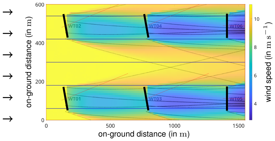
Figure 1 Simulation of the local wind speed (in m s⁻¹) with six turbines (of type NREL 5 MW) arranged in a 2×3 grid layout; axes give on-ground distances (in m). The wind blows from west to east with a speed of 11 m s⁻¹ and a turbulence intensity of 6 %. It is decreased by the turbines, and, additionally, the wakes are deflected by the turbines in the first and second columns because of their yaw offset of 15°. (The downstream-most turbines have a yaw offset of 0°.) This figure was produced using the software WinFaST; see Sect. 3.1 for a description.

In the following, we discuss the wake models, farm layouts, and farm operations to motivate the wind farm yaw problem and discuss our approach along with contributions and limitations; an outline of the remainder of the paper concludes this introduction.

The remainder of the paper is structured as follows. In Sect. 2, we formulate the wind farm yaw problem (WFYP) mathematically, and we motivate and develop our covering approach (CA) and the corresponding integer program (IP). The details on precomputations, i.e., on the simulation and the resulting performance indicators, are described in Sect. 3. We explain and discuss the results of our computational experiments in Sect. 4 and, finally, conclude in Sect. 5. The theoretical complexity of the WFYP is examined in Appendix A. We use the abbreviations farm for wind farm, turbine or WT for wind turbine, and TI for turbulence intensity.

1.1 Related work

Wake models in the literature are often parameterized to NREL 5 MW turbines, see Jonkman et al. (2009) for details, in usual atmospheric conditions for onshore wind farms; see Sect. 3.1 for details. The following brief survey refers to this turbine type; for a detailed overview of the complex topic of wind farm flow control, we refer to, e.g., Meyers et al. (2022). High-fidelity simulations of wind farms in 3D, such as the Simulator fOr Wind Farm Application (SOWFA), see Churchfield et al. (2012a, b) and Fleming et al. (2013), are time-consuming and, hence, impractical for use in control. An overview of the most important control-oriented models in 2D is given in Annoni et al. (2018) (their Sect. 2.1): first, the Jensen model (see Jensen, 1983, and Katic et al., 1987) (also for a further developed model); second, the multi-zone model FLORIS (see Gebraad et al., 2014), which has the dynamic extension FLORIDyn (see Gebraad and van Wingerden, 2014); and third, the Gaussian model (see, e.g., Bastankhah and Porté-Agel, 2016). These models are continuously being developed. In the present work, we use a simulation software which utilizes a wake model based on FLORIDyn; see Sect. 3. State-of-the-art static wake models are the Gauss–curl hybrid model, which incorporates secondary effects of wake steering, see King et al. (2021), and the cumulative-curl wake model, if there are more than a few wake interactions; see Bay et al. (2023). Both are implemented in the rapidly evolving software FLORIS (not to be confused with the original model), incorporating several steady-state control-oriented wake models; see NREL (2024). These control-oriented wake models have limitations: for a comparison between FLORIDyn and SOWFA, we refer to Gebraad and van Wingerden (2014). In any case, the mathematical approach we propose utilizes a superordinate model, in which the underlying wake model is interchangeable.

A profitable wind farm needs a suitable location and careful planning of turbine numbers and placement. Wind farm layout optimization relies on yearly wind frequency data (wind direction and speed). It has been known for decades that it is useful to avoid wake-induced yield reductions of downstream turbines by setting them far enough apart; see, e.g., Katic et al. (1987). While first attempts to account for such effects merely simulated the annual average output of a specific farm layout, see Katic et al. (1987), in recent years, the layout problem was optimized globally by mixed-integer and constraint programming; see, e.g., Zhang et al. (2014), Fischetti (2017), and Fischetti (2021). In addition to the annual energy output, noise propagation is a concern in the case of onshore farms and can also be considered; see Zhang et al. (2014). For offshore farms, aspects such as cable routing and jacket foundations are worth taking into account; see Fischetti (2017) and Fischetti and Pisinger (2019).

For a given wind farm (i.e., a fixed layout), it is conventional to run greedy control for each individual turbine; see, e.g., Hau (2013). As mentioned earlier, adopting a global control for the whole farm instead of local control of separate turbines can potentially improve the overall power output and relieve physical strain on the turbines. In general, there are two common global control concepts (cf. e.g., Gebraad et al., 2015; Annoni et al., 2016; Meyers et al., 2022): axial-induction-based control (of generator torque and/or the collective blade pitch angle) and yaw-based control (of the turbine yaw offsets), which is also known as wake steering control; see, e.g., Howland et al. (2019). Both control concepts effectively reduce power generation of upstream turbines by adjusting torque/pitch or yaw, respectively, which in turn leads to increased wind speeds (relative to those under greedy control) in their respective wakes and, consequently, a higher power yield of the affected downstream turbines. The main aim of these concepts is to achieve a net gain, and even small improvements are deemed promising; see, e.g., the wake steering study by Howland et al. (2022) with average power increases of 0.3 % to 2.7 % for a commercial wind farm.

In general, whether a control different from the greedy one can indeed yield the desired gains depends on the allocation of the turbines, their characteristics, and the wind conditions: e.g., it may happen that wind speeds are so high that all turbines operate at maximal capacity anyway; nevertheless, some control could still be meaningful to reduce mechanical loads. Further, there are cases in which axial induction control shows no positive effect on total power output, while farm-level yaw control yields significant improvements; see the high-fidelity computational fluid dynamics simulations in Gebraad et al. (2015). Thus, we focus on farm-level yaw control in this paper, where changing the yaw offset of a turbine deflects its wake.

There is already a lot of research on yaw-based control. We follow the literature distribution in Stanley et al. (2022), which divides yaw-based control into two parts to tackle the optimization problem, i.e., using continuous yaw offsets between lower and upper bounds (see Gebraad et al., 2014; Fleming et al., 2016; Gebraad et al., 2017) and using discretized yaw offsets (see Dar et al., 2017, and Dou et al., 2020). In Gebraad et al. (2014), a slow game-theoretic approach is used, which does not necessarily deliver a global optimum as desired. This is also not delivered in Fleming et al. (2016) and Gebraad et al. (2017) as their optimization method is based on sequential quadratic programming (SQP). However, a combination of farm-level yaw control and farm layout optimization has been considered in both studies, which is an interesting application but out of the scope of the present paper. In Dar et al. (2017), the authors modified the Jensen model (cf. Jensen, 1983) to include the effect of yaw offset adjustments and developed a dynamic programming formulation (DPF) to pass the wind speed downstream from turbine to turbine, which results in a very efficient method for turbines in a single row. However, the nonlinearity of the equation used to compute the wind speed for a turbine located in several turbine wakes prevents the transferral of this concept to a 2D farm layout. Nevertheless, Dar et al. (2017) showed that optimizing each row separately with DPF, i.e., ignoring effects in adjacent rows, reduces the gap between its so-called wind farm efficiency and its globally optimal quantity (obtained by full enumeration) to up to 1 %.

This idea to split the farm into disjoint subsets of turbines has already been presented in Spudić and Baotić (2013), which tackles distributed systems, and is also used in Siniscalchi-Minna et al. (2020), Bernardoni et al. (2021), and Dong and Zhao (2023). The latter paper even allows at least one turbine per subset to be in several subsets, which can lead to conflicting yaw offsets: while they describe a supporting logic to handle this, we inherently ensure yaw offset compatibility for any number of turbines. Our goal is to determine the global optimum – under some mild assumptions, see Sect. 1.2.1 for details – without resorting to full enumeration; for this, our superordinate model takes dependencies of adjacent subsets of turbines into account and can integrate any kind of wake effect simulation.

In fact, we regard the farm as a network. This general point of view has already been used in Annoni et al. (2019) for a different application, namely to share information among nearby turbines to improve wind direction estimation; the underlying method, which allows simultaneous clustering and optimization on graphs, was developed in Hallac et al. (2015). In Dou et al. (2020), the covariance matrix adaptation evolution strategy is employed, which is a heuristic algorithm for black-box functions. In contrast, our focus is to exploit the structure of the optimization problem. In Stanley et al. (2022), the structure of the problem is used in the new so-called Boolean approach. This considers which turbines have downstream turbines in their wake, starts at the upstream-most turbine, and fixes a yaw offset to either 0° or 20° if it increases the power of the farm; the simulations used the software FLORIS (cf. NREL, 2024) with the Gauss–curl hybrid wake model (cf. King et al., 2021). The so-called serial-refine method, see Fleming et al. (2022), is based on the Boolean approach, whereby each turbine is run through twice (in a serial and a refine pass), which allows several yaw offsets. This method is both fast and successful and is suitable for comparison, even if it generally does not guarantee a globally optimal solution. In contrast, our approach optimizes yaw offset settings simultaneously for the whole farm. (From the view of blade load, which we do not take into account, a slightly positive yaw offset is best, whereas the exact location depends on the level of wind shear; see the field study of Ennis et al., 2018.)

1.2 Contributions and limitations

We provide a method of globally optimal farm-level yaw control (under some mild assumptions) that also includes the possibility to deactivate wind turbines, e.g., for maintenance reasons. To that end, we propose a novel superordinate model which exploits the coupled nature of wind turbines in a wind farm and can be based on any wake model.

We refer to the determination of a globally optimal combination of yaw offsets for a given wind farm layout and given wind conditions (i.e., subject to arbitrary but fixed wind speed and direction) as a WFYP; see Sect. 2 for details and a mathematical problem definition. In this context, global optimality refers to an objective function, which takes the total power output of the farm into account – our main goal – and can include other quantities representing mechanical loads; in fact, we include the important tower load and the pitch angle changes (causing some wear) as so-called tower activity and pitch activity (see Sect. 3 for a definition), and we do not consider the blade load, as the simulation software used, described in Sect. 3.1, does not provide a suitable output quantity.

The complex nonlinearities of wake flow dynamics and turbulence are typically only available through simulation, which makes a direct integration into an optimization model almost impossible. A naive approach to solving the WFYP is to run simulations for every possible yaw offset combination, i.e., full enumeration, but this is already impractical for small farms. A crucial observation is that the wake interactions of turbines adhere to certain patterns with respect to the farm layout that occur repeatedly, and with overlaps, across the entire farm. We exploit these redundancies to greatly reduce the number of required combinations: our superordinate model constructs the farm on the basis of these patterns of dependent turbines and ensures consistency in selected yaw offsets in regions of overlapping patterns; we formulate a corresponding IP to yield the desired yaw offsets as a solution.

Our numerical experiments are intended as proof of concept as we use error-free simulation data. They show that state-of-the-art solver software for this problem class – e.g., Gurobi, see Gurobi Optimization (2022), or SCIP, see Bestuzheva et al. (2021) – can solve these WFYP problems within a reasonable time frame, demonstrating the practicality of our approach.

The use of our superordinate model enables the deactivation of any turbines and a large scaling of the wind farm size orthogonal to the wind direction, whereas a scaling in wind direction significantly increases the computational effort due to a stronger growth of relevant patterns – while it is beyond the scope of this paper, scaling in the wind direction is possible through the following: split the patterns into segments in the wind direction (rows of turbines, so to speak), compute the upstream-most segment with specific yaw offsets, run the simulation, save the resulting wind field, use it to simulate all yaw offset combinations in the next segment, and so on. Moreover, the weighting flexibility of the objective function terms (power output and mechanical loads) allows additional objectives to be considered, e.g., putting selected turbines in a low-load operating mode.

1.2.1 Assumptions

We consider the setting in which all turbines in the wind farm are of the same type and are arranged on an underlying irregular grid. These assumptions are not particularly restrictive in practice since, on the one hand, turbines within one farm are typically of the same type – although layout optimization can result in different turbine heights, see, e.g., Stanley et al. (2017) – and, on the other hand, we can, in principle, choose the grid resolution as fine as needed to allow for the representation of any layout (by leaving some grid points unused); e.g., the results of layout optimization in Thomas et al. (2015) and Gebraad et al. (2017) are not arranged on a simple grid. However, an irregular grid with, e.g., 3 and 5 rotor diameter distance between the turbines is quite common, see, e.g., Gebraad et al. (2014), Gebraad and van Wingerden (2014), Boersma et al. (2018), and Boersma et al. (2019b).

Moreover, our model of the WFYP problem relies on two operational assumptions, which can also be realized with arbitrarily fine resolution and should therefore not be restrictive in applications: the admissible yaw offsets are bounded – to prevent overly strong mechanical loads, cf. e.g., Boersma et al. (2019a) – and discretized, and we impose a threshold below which the influence of wakes on downstream turbines is deemed negligible.

In particular, Fleming et al. (2016) limit the yaw offset to $[-\mathrm{45}\mathit{°},+\mathrm{45}\mathit{°}]$ and $[-\mathrm{25}\mathit{°},+\mathrm{25}\mathit{°}]$, Boersma et al. (2019a) to $[-\mathrm{25}\mathit{°},+\mathrm{25}\mathit{°}]$, and Stanley et al. (2022) to [0°,30°], and our industry partner suggests $[-\mathrm{15}\mathit{°},+\mathrm{15}\mathit{°}]$ to protect the turbines. In our computational experiments, e.g., we choose yaw offsets from $[-\mathrm{15}\mathit{°},+\mathrm{15}\mathit{°}]$ at 5° increments and set the downstream-most turbines to 0° (to reduce the number of options, see Sect. 2.1) – we always state yaw offsets relative to the (fixed) wind direction, i.e., as yaw offsets with respect to the mathematically positive sense of rotation. Further, we accept small model inaccuracies by disregarding wake influence if the wake-induced wind speed reduction (relative to the free stream) at the downstream turbine is small; see Sect. 2.2.1 for details. We also refer to this exemplary setup for illustrative purposes when we formally define the WFYP and our solution approach in Sect. 2. Nevertheless, our method allows other arbitrary settings, e.g., discretized yaw offsets for the downstream-most turbines.

Our choice is not unrealistic: Quick et al. (2020) describe the problem of uncertainty in incident wind conditions for metrological reasons and for real-world causes; in fact, the inflow of a wind farm can consist of several wind directions, speeds, TIs, and shears (e.g., caused by a mountain). Stanley et al. (2022) deduce that it is unrealistic to solve the WFYP with continuous or finely discretized yaw offsets and choose their Boolean optimization approach based on the idea that they only have to decide whether a turbine is yawed or not, i.e., set 0° or 20° (which is a result of power simulations of turbines with a yaw offset discretization of 5°); they also compared their approach with a common continuous yaw optimization (based on gradients) and mostly achieve the same power improvement. Against this background, our choice of 5° increments is reasonable.

In general, wind turbulence depends on a number of meteorological and topographical factors, whereas power output essentially depends on long-term fluctuations, and loads are caused by short-term fluctuations; see Hau (2013). We fix the TI, see Sect. 3.1 for a definition, throughout this paper; for an illustration of the locally strong speed fluctuations in the wind field, see Fig. 1. For general effects we refer to Talavera and Shu (2017): first, there is a correlation between the increase in TI and faster wake recovery (as wind speed recovers faster for turbulent shear flow in comparison to laminar shear flow), and, second, turbulent inflow increases the power output of a wind turbine (because of suppressed flow separation).

The correlation between important weather characteristics, like temperature, relative humidity, wind speed, and wind gusts, are investigated in Vladislavleva et al. (2013) (their Fig. 2): as expected, wind speed and gusts have a strong positive correlation with power output, while pressure has a slightly negative one. Finally, the spectrum of possible influences is wide. We focus here on the most influential factors, i.e., wind speed and direction, and fix the others, like TI and air density, for simplicity.

1.2.2 Complexity theory point of view and computation time

In fact, while the described homogeneous turbine type and layout structure and the yaw offset discretization may seem to simplify the problem, this is not the case from the viewpoint of computational complexity theory: as we prove in Appendix A, the WFYP is generally 𝒩𝒫 hard, which means that an efficient solution algorithm – i.e., one with a run time polynomially bounded by the input size – is highly unlikely to exist; cf. Garey and Johnson (1979). This computational intractability result, along with discretization-related aspects, motivates and justifies tackling the WFYP using IP techniques; see, e.g., Schrijver (1986) for a thorough introduction to IPs.

Thus, the only remaining potentially limiting aspect is the computation time, which naturally increases with growing problem size and complexity. The assessment of Fleming et al. (2022) for a real-time control is at the timescale of seconds to minutes. Nevertheless, in general, we can exploit two mitigating facts: first, it is useful to avoid continuous, small yaw movements in order to not unduly increase mechanical loads, and, second, the yawing rate must be slow (approximately 0.5 ° s⁻¹) to avoid gyroscopic moments; see Hau (2013) (their Sects. 6.3.1 and 11.3). As a consequence, we assume that a computation time of less than 1 min is sufficient; in addition, a light detection and ranging (lidar) system could provide wind information at an early stage. As our IP approach is capable of determining globally optimal yaw offset combinations for entire farms of considerable size at most under 1 min (after required precomputations), e.g., 27 wind turbines in 11 s, it is suitable for real-world application. However, the practical realization of a short real-time control scale would require a time-delayed yaw offset adaption of each turbine (depending on the propagation time). In our computational experiments, we do not consider this transient phase but rather the effects over a longer period of time, namely 10 min; see Sect. 3.2 for details.

2 The wind farm yaw problem

Recall that our WFYP aims to find a set of yaw offsets that maximizes the total power output of the farm, optionally along with other quantities, under a given wind scenario, i.e., fixed wind direction and speed. We formalize this optimization task in Sect. 2.1, develop our CA in Sect. 2.2, and derive the corresponding IP in Sect. 2.3.

2.1 Notation, basic WFYP formulation as IP with black-box objective, and the curse of dimensionality

We consider a farm with n_WT turbines, each identified by an index from the set $T:=\mathit{\{}\mathrm{1},\mathrm{2},\mathrm{\dots },n_{\mathrm{WT}}\mathit{\}}$. Later, in Example in Sect. 2.1, we use our ultimate assumption that turbines are located on an irregular grid with certain spacing in both dimensions. We assign to each turbine i∈T a set Γ_i of admissible yaw offsets, see Sect. 1.2.1, with respective size $n_{\mathrm{\Gamma },i}:=\left|{\mathrm{\Gamma }}_i\right|<\mathrm{\infty }$. For every turbine i, we associate an index set $N_{\mathrm{\Gamma },i}:=\mathit{\{}\mathrm{1},\mathrm{\dots },n_{\mathrm{\Gamma },i}\mathit{\}}$ with its admissible yaw offsets. This general notation allows for turbines of different types, but even when working with identical turbines, for which the yaw offset sets usually coincide, differences may arise, e.g., if maintenance reasons limit the options for specific turbines.

Recalling that turbines can influence each other, the overall power output of the farm and other load-related quantities depend on the global yaw configuration, i.e., the collection of the set yaw offsets of all individual turbines and the considered wind conditions (in particular, direction and speed). Since the precise relation of these aspects has no known analytical form, the objective function of the WFYP must generally be considered a black box, whose values for a specific combination of input parameters can be determined, or estimated, by running a simulation of the corresponding farm scenario.

To specify a basic mathematical formulation of the WFYP, we introduce binary decision variables x_i,j for all i∈T, $j\in N_{\mathrm{\Gamma },i}$; if turbine i is set to the yaw offset (from Γ_i) indexed by j, then $x_{i,j}=\mathrm{1}$, and otherwise $x_{i,j}=\mathrm{0}$. As any turbine can only operate with one yaw offset at a time, these decision variables must adhere to ${\sum }_{j\in {\mathrm{\Gamma }}_i}{x}_{i,j}=\mathrm{1}$ for all i∈T. The black-box objective can then be described by a function $f_{\mathit{\omega }}:\mathit{\{}\mathrm{0},\mathrm{1}{\mathit{\}}}^{n_{\mathrm{\Gamma },\mathrm{1}}+\mathrm{\dots }+n_{\mathrm{\Gamma },n_{\mathrm{WT}}}}\to {\mathbb{R}}^{n_{\mathrm{WT}}}$, where we omit the dependency on the (here, fixed) wind direction and speed as well as farm layout for notational convenience and where the vector ω consists of two weighting factors, which we discuss later. This function is comprised of the objective contribution of every turbine, which is impacted by its own yaw offset and the yaw configuration of the remaining farm (in fact, not all other turbines influence any given turbine, but for now, we do not utilize this). In particular, the function $f_{\mathit{\omega }}\left(x\right)=\left(f_{\mathit{\omega },\mathrm{1},j_{\mathrm{1}}}\right(x),\mathrm{\dots },f_{\mathit{\omega },n_{\mathrm{WT}},j_{n_{\mathrm{WT}}}}(x){)}^{\top }$, where $f_{\mathit{\omega },i,j}\left(x\right)$ denotes the objective contribution of turbine i when set to yaw offset index j from its admissible set Γ_i (as per $x_{i,j}=\mathrm{1}$). Here, the yaw configuration of all turbines (in particular those that influence i) is fixed, as prescribed by the decision variables x. To find the optimal yaw configuration of all turbines, i.e., a solution $x\in \mathit{\{}\mathrm{0},\mathrm{1}{\mathit{\}}}^{n_{\mathrm{\Gamma },\mathrm{1}}+\mathrm{\dots }+n_{\mathrm{\Gamma },n_{\mathrm{WT}}}}$, our objective function sums up contributions of individual turbines:

$$\begin{array}{}\text{(1)}& f_{\mathit{\omega }}^{\mathrm{\Sigma }}\left(x\right):=\sum _{i=\mathrm{1}}^{n_{\mathrm{WT}}}\sum _{j=\mathrm{1}}^{n_{\mathrm{\Gamma },i}}{f}_{\mathit{\omega },i,j}\left(x\right)x_{i,j}\end{array}$$

with black-box simulation function

$$\begin{array}{}\text{(2)}& f_{\mathit{\omega },i,j}\left(x\right):=P_{i,j}\left(x\right)-{\mathit{\omega }}^{\left(\mathrm{T}\right)}{a}_{i,j}^{\left(\mathrm{T}\right)}\left(x\right)-{\mathit{\omega }}^{\left(\mathrm{P}\right)}{a}_{i,j}^{\left(\mathrm{P}\right)}\left(x\right),\end{array}$$

where P_i,j, $a_{i,j}^{\left(\mathrm{T}\right)}$, and $a_{i,j}^{\left(\mathrm{P}\right)}$ are the average power output, the tower activity, and the pitch activity – all over a certain (fixed) period of time – of turbine i∈T, with yaw offset index j∈Γ_i (and the remaining yaw offsets corresponding to the selections encoded in x). To evaluate the black box for a specific x, one needs to resort to simulation to obtain the power and mechanical load values for each turbine in the considered farm (under the given wind scenario) – the details, including definitions of the notions of tower and pitch activity, are described in Sect. 3. The (nonnegative) weighting factors ω^(T) and ω^(P) are set a priori and determine the relative importance of the respective quantities in the optimization objective; in particular, both weights can be set to zero to take only the power into account. In addition, we could choose individual weights for each turbine.

Thus, we formulate the WFYP as an IP with the following black-box objective:

$$\begin{array}{}\text{(3)}& {\displaystyle }\underset{x}{max}& {\displaystyle }\sum _{i=\mathrm{1}}^{n_{\mathrm{WT}}}\sum _{j=\mathrm{1}}^{n_{\mathrm{\Gamma },i}}{f}_{\mathit{\omega },i,j}\left(x\right)x_{i,j},\text{(4)}& {\displaystyle }\text{ s.t.}& {\displaystyle }\sum _{j=\mathrm{1}}^{n_{\mathrm{\Gamma },i}}{x}_{i,j}=\mathrm{1}\text{ for }i=\mathrm{1},\mathrm{\dots },n_{\mathrm{WT}},\text{(5)}& {\displaystyle }& {\displaystyle }{x}_{i,j}\in \mathit{\{}\mathrm{0},\mathrm{1}\mathit{\}}\text{ for }i=\mathrm{1},\mathrm{\dots },n_{\mathrm{WT}}\text{and}j=\mathrm{1},\mathrm{\dots },n_{\mathrm{\Gamma },i}.\end{array}$$

Due to the black-box nature of the objective function, the above formulation cannot simply be handled by off-the-shelf IP solvers. Indeed, we call it the “basic” formulation because it essentially requires computing all $f_{\mathit{\omega },i,j}\left(x\right)$ values to obtain a standard (non-black-box) IP and hence corresponds to the naive brute-force full enumeration. Clearly, this approach is only viable for very small WFYP instances – i.e., few turbines with a small set of admissible yaw offsets – due to the exponential growth of yaw offset combinations; see also Remark in Sect. 2.1. Moreover, each simulation run incurs a certain run time that itself increases with the farm size. Thus, the WFYP suffers from the typical “curse of dimensionality” often encountered in combinatorial problems. In fact, our following result establishes that an efficient (polynomial-time) solution method for the WFYP very likely does not exist; the proof is deferred to Appendix A.

Proposition

Theorem A4 and Corollary A6 from Appendix A. The WFYP is strongly 𝒩𝒫 hard and cannot be approximated within any factor α≤1 in polynomial time (unless 𝒫=𝒩𝒫).

Example

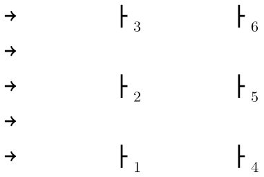
A 3×2 farm. We consider n_WT=6 turbines, arranged in a 3×2 farm (see Fig. 2); we assume the wind blows from west to east, and we identify the turbines with the index set $T=\mathit{\{}\mathrm{1},\mathrm{\dots },\mathrm{6}\mathit{\}}$. The turbines may be homogeneous, consisting of NREL 5 MW turbines with a rating value of 5 MW and a rotor diameter of D=126 m; cf. Jonkman et al. (2009) (their Table 1-1). We set the turbine spacing to 3D×5D; i.e., turbines are on an irregular grid with 3 and 5 rotor diameter distance between turbines in the width (“column”) and depth (“row”) directions, respectively. We choose the notation analogous to matrices; in the literature, our example would usually be referred to as 2×3 with 5D×3D. However, the spacing choice is common, see, e.g., farms in Gebraad et al. (2014), Gebraad and van Wingerden (2014), Boersma et al. (2018), and Boersma et al. (2019b) (also, Katic et al., 1987, mentions 5D as a row value but no column value). We restrict the permissible yaw offsets to ${\mathit{\gamma }}_i\in {\mathrm{\Gamma }}_i=\mathrm{\Gamma }:=\mathit{\{}-\mathrm{15}\mathit{°},-\mathrm{10}\mathit{°},\mathrm{\dots },+\mathrm{15}\mathit{°}\mathit{\}}$ and $n_{\mathrm{\Gamma },i}=n_{\mathrm{\Gamma }}:=\mathrm{7}$ for every i∈T (cf. Sect. 1.2.1).

Figure 2 Illustration of the 3×2 farm layout from Example in Sect. 2.1; the wind direction is indicated by the small arrows. The drawing is true to scale for NREL 5 MW turbines, which have a rotor diameter of D=126 m, and for a turbine spacing of 3D×5D.

Remark

Total number of possible yaw configurations of a 3×2 farm. Example in Sect. 2.1 yields a total number of $n_{\mathrm{\Gamma }}^{n_{\mathrm{WT}}}={\mathrm{7}}^{\mathrm{6}}=\mathrm{117}\mathrm{649}$ possible yaw configurations. Consequently, this number of farm simulations would be required to solve the WFYP with the basic approach for one wind scenario. Therefore, we need a different approach to reduce the number of simulations. A coarser yaw offset discretization is not an option as it would sacrifice the level of exercisable control. Indeed, our approach achieves this by reducing the number of yaw offset combinations to consider and by reusing simulation results where possible.

A turbine has the highest power output with a yaw offset of 0° (i.e., it runs greedily); see, e.g., Dar et al. (2017). Therefore, an initial approach that most likely preserves the most power output but reduces the number of options is to let the downstream-most turbines run greedily. (We verified this through an experiment in which the wake of a yawed turbine had no influence on this approach at a distance of 3D.) The number of possible yaw configurations in Example in Sect. 2.1 would then decrease to 7³=343; however, such an approach does not scale – a 3×3 farm again results in 7⁶ configurations. This emphasizes the need for an altogether different approach.

2.2 Covering approach for WFYP solution

The assumed homogeneous turbine type and layout structure give rise to recurring patterns that can be exploited to equivalently reformulate the WFYP in a way that reduces the number of black-box evaluations (i.e., simulation runs).

2.2.1 Upstream sections

To that end, we take a closer look at the turbines that influence a specific turbine, i.e., affect the latter by the downstream wind wake; we call the set of turbines that influence a specific turbine an upstream section (including the specific turbine). The size depends on the wind conditions (in particular, the wind direction) and the yaw offset(s) of the influencing turbine(s). It includes all turbines that could influence an upstream section, namely the specific turbine in focus; i.e., the upstream section is based on the admissible yaw offset ranges. Moreover, we remind the reader that one assumption is to accept small model inaccuracies by disregarding wake influence if the wake-induced wind speed reduction at the downstream turbine is small; see Sect. 1.2.1. The concrete chosen area is a trapezoid (for visualization we sometimes use triangles), see Fig. 3, with a minimum absolute slope value of 0.15, which corresponds to approximately 8.5°. (For a rough comparison, Dar et al., 2017, neglect the deficit in velocity for yaw offsets beyond 20° from the center of the turbine based on Jensen, 1983.) We increase the slope until all so-called observation points in the wake from simulations with WinFaST software (with 0° and extreme yaw offsets, e.g., ±15°), see Sect. 3.1, with a wind speed deficit larger than 5 % are in the trapezoid. The depth of this trapezoid is usually truncated (or, rarely, extended) to match the depth of the farm – in fact, we use the effective depth of the farm, which we define in Sect. 2.2.3; it coincides with the depth of the farm if the wind direction is 0° and can be smaller otherwise. Finally, this simply constructed trapezoid turned out to be a suitable upstream section: we successfully compare our CA with full enumeration in Sect. 4.

To illustrate upstream sections, reconsider Example in Sect. 2.1 and its farm in Fig. 2. Under these fixed wind conditions, WTs 1, 2, and 3 influence WT 5 depending on the yaw offsets in $[-\mathrm{15}\mathit{°},+\mathrm{15}\mathit{°}]$; i.e., the upstream section at WT 5 is given by $\mathit{\{}\mathrm{1},\mathrm{2},\mathrm{3},\mathrm{5}\mathit{\}}$. The chosen upstream section is useful for explaining the concept. In fact, with the selected experimental setup for our results in Sect. 4, the corresponding upstream section would only include WTs 2 and 5; see Fig. 3a for a corresponding farm with three turbines in depth and Fig. 3 for an overview with wind directions of 0, 5, 10, and 20°.

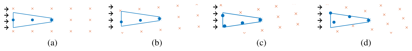
Figure 3 Upstream sections (blue trapezoids) with included turbines (marked as points; asterisks are the downstream-most turbine in the upstream section) in a grid of turbines (red crosses) for (a) 0, (b) 5, (c) 10, and (d) 20°. The grid represents a farm with infinite expansion.

2.2.2 Section configurations

Depending on the positions of subsets of turbines within the farm (keeping all other aspects fixed), upstream sections can take on different patterns, which can be identified based solely on the grid layout of the farm; see, e.g., Fig. 4. In particular, we can omit (or deactivate) turbines within any upstream section, thereby obtaining what we call section configurations as structural subsets of the complete section configuration, i.e., the upstream section itself. Crucially, if all turbines are of the same type, only a single upstream section is needed as a “template” from which to extract the appropriate “patterns” with which the farm can be represented – i.e., we can cover the entire farm using (overlapping) section configurations – and simulations can focus on the upstream section (reusing simulation results of the section configurations) rather than the whole farm directly. After the following example, we formalize and explain this covering approach.

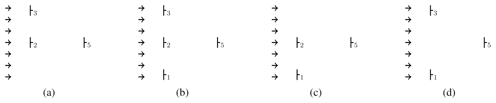
Figure 4 Example of some section configurations of the upstream section with $n_{\mathrm{WT},u}=\mathrm{4}$ turbines: (a) section configuration with inactive WT 1, (b) complete section configuration (i.e., upstream section), (c) section configuration with inactive WT 3, and (d) section configuration with inactive WT 2. We kept the numbering from Fig. 2, but the depicted patterns may and do occur in other parts of the farm as well.

We can cover the 3×2 farm from Example in Sect. 2.1 (cf. Fig. 2) by the section configurations shown in Fig. 4: we anchor the configuration from (b) at WT 5 and the configurations from (a) and (c) at WTs 4 and 6 (as the respective downstream-most turbine instead of 5), respectively, since the corresponding parts of the farm exhibit the same structural pattern; see also Fig. 5a. A change in the farm layout would require other section configurations; e.g., without WT 2, we would need the configuration depicted in Fig. 4d for WT 5 and the one with just two turbines directly behind each other (not depicted) for WTs 4 and 6. In total, for the upstream section, we have 16 possible section configurations, including the complete one and the empty one. In general, if an upstream section encompasses n_WT,u turbines, there is a total of ${\mathrm{2}}^{n_{\mathrm{WT},u}}$ possible section configurations.

As in the example, we only need a small number of the possible section configurations to cover the farm during normal operation. However, we take into account all possible section configurations: it increases the precomputation time but preserves flexibility; i.e., we are prepared for deactivated turbines and can enlarge the farm orthogonal to the wind direction.

2.2.3 Covering sections to reduce the computational burden

To formalize the notion of section configurations that are suitable for covering the farm, it suffices to focus on the downstream-most turbines, whose number we denote as n_s, and determine so-called covering sections anchored at them.

Definition

Covering sections. A covering section is a set S_k⊆T of turbines in a farm that influence each other with respect to (wake) disturbances. We denote the set of covering sections in a farm as $S:=\mathit{\{}{S}_{\mathrm{1}},\mathrm{\dots },S_{n_{\mathrm{s}}}\mathit{\}}$. Furthermore, we denote the set of covering sections that contain a specific turbine i as $S\left(i\right):=\mathit{\{}{S}_k\in S:i\in S_k\mathit{\}}$.

Remark

To cover the farm, we must assign one covering section to each downstream-most turbine, as illustrated in Fig. 5, but as different covering sections can have the same pattern, a section configuration can be used several times, e.g., in Fig. 5b. The core advantage of this CA is the significantly reduced number of simulations required to find the best WFYP solution (in comparison to full enumeration) as we only need to precompute the yaw configurations within every (distinct) section configuration and, accordingly, obtain the simulation results for all covering sections.

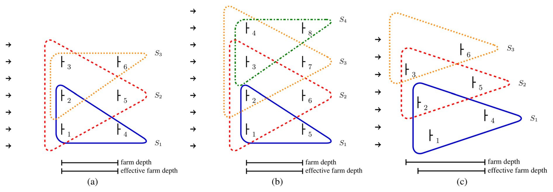
Figure 5 Covering sections $S_{\mathrm{1}},\mathrm{\dots },S_{\mathrm{3}}$ in a 3×2 farm and $S_{\mathrm{1}},\mathrm{\dots },S_{\mathrm{4}}$ in a 4×2 farm, where S₁ is outlined by the solid blue line, S₂ by the dashed red line, S₃ by the dotted orange line, and S₄ by the dash-dotted green line. (a) In a 3×2 farm, S₁ (anchored at WT 4) uses the section configuration (SC) from Fig. 4a to cover WTs $\mathit{\{}\mathrm{1},\mathrm{2},\mathrm{4}\mathit{\}}$, S₂ (at WT 5) employs the SC from Fig. 4b for $\mathit{\{}\mathrm{1},\mathrm{2},\mathrm{3},\mathrm{5}\mathit{\}}$, and S₃ (at WT 6) uses the SC in Fig. 4c for $\mathit{\{}\mathrm{2},\mathrm{3},\mathrm{6}\mathit{\}}$. (b) In a 4×2 farm, S₁ (anchored at WT 5) uses the SC from Fig. 4a to cover WTs $\mathit{\{}\mathrm{1},\mathrm{2},\mathrm{5}\mathit{\}}$; both S₂ and S₃ (at WTs 6 and 7, respectively) use the SC from Fig. 4b for $\mathit{\{}\mathrm{1},\mathrm{2},\mathrm{3},\mathrm{6}\mathit{\}}$ and $\mathit{\{}\mathrm{2},\mathrm{3},\mathrm{4},\mathrm{7}\mathit{\}}$, respectively; and S₄ (at WT 8) uses the SC from Fig. 4c for $\mathit{\{}\mathrm{3},\mathrm{4},\mathrm{8}\mathit{\}}$. (c) In a 3×2 farm with a wind direction of 20°, S₁ to S₃ are sufficient to cover the farm, although their depth coincides with that of the upstream section, which is smaller than that of the farm.

We have already mentioned that wind directions deviating from 0° require us to define the effective depth of the farm. For illustration, we use a 3×2 farm with a wind direction of 0 and 20°; see Figs. 5a, c. In the case of 0°, the farm and the corresponding upstream section both have a depth of 5D. For other directions, e.g., as in Fig. 5c, this depth changes. The depth of the farm is the distance in the x direction between the upstream- and downstream-most turbines inside the farm, i.e., in our example between WTs 3 and 4. The depth of the upstream section is analogously defined inside the upstream section – in our example, WTs 2 and 4. As this depth is sufficient to finally cover the farm, we also call it the effective depth of the farm. Usually, our use of the terms “upstream-” and “downstream-most” turbines refers to these covering sections; e.g., in our example, WTs 4 to 6 are the downstream-most ones and serve as anchors for the covering sections. If an anchor turbine is missing, say WT 4, we relocate the covering section; i.e., in our example, we attach S₁ at WT 1 (where S₁ uses the section configuration with only one active turbine). Then we can assume without loss of generality that the downstream-most turbine inside a non-empty section configuration is always active, thus circumventing half of all combinations in which the downstream-most turbine could be inactive. (Alternatively to this relocation, one could have anchored the covering section at a deactivated “virtual” WT 4.)

2.2.4 The required number of simulations

Before we turn to the WFYP model based on the CA, we take a closer look at the required number of simulations to solve it. For simplicity, we assume the same set of admissible yaw offsets, say, Γ with $n_{\mathrm{\Gamma }}:=\left|\mathrm{\Gamma }\right|$ for the (identical) turbines. In the basic approach for the whole farm with n_WT turbines, we see in Remark in Sect. 2.1 that the total number of distinct yaw configurations, which coincides with the required number of simulations, amounts to $n_{\mathrm{\Gamma }}^{n_{\mathrm{WT}}-n_{\mathrm{s}}}$ if the n_s downstream-most turbines run greedily. Analogously, again running the downstream-most turbine greedily, an upstream section with n_WT,u turbines allows $n_{\mathrm{\Gamma }}^{n_{\mathrm{WT},u}-\mathrm{1}}$ possible yaw configurations and a covering section S_k with n_WT,k turbines allows $n_{\mathrm{\Delta },k}:=n_{\mathrm{\Gamma }}^{n_{\mathrm{WT},k}-\mathrm{1}}$.

To solve a single WFYP instance, we perform precomputations, i.e., simulation runs for all yaw configurations on all possible section configurations; recall that we include all possible section configurations (not only those that occur as covering sections) to preserve flexibility (see Sect. 2.2.2), and thus, we derive the worst-case number of simulations. In addition to remembering that farm layout and wind conditions (in particular, direction and speed) are fixed for a single WFYP instance. Consequently, while the number of simulations for each scenario is much lower than in the basic approach, preparing our approach for application in a variety of wind scenarios for a given farm will still result in a large precomputation time to run all required simulations. However, we propose storing these precomputed simulation results in a database so that data corresponding to any currently encountered scenario can be retrieved efficiently to solve the corresponding WFYP instance in order to update the yaw control.

In the following, we derive the number of combinations (section configurations and corresponding yaw configurations) and the required number of simulation runs. As there are different ways to avoid further redundant computations in specific situations, these numbers are upper bounds and might be further reduced; we mention some examples of this aspect.

An upstream section (i.e., complete section configuration) with n_WT,u turbines has ${\mathrm{2}}^{n_{\mathrm{WT},u}}-\mathrm{1}$ non-empty section configurations. All other section configurations have fewer active turbines than n_WT,u and, consequently, allow fewer possible yaw configurations (than the complete one); i.e., the number of required simulation runs is smaller than $({\mathrm{2}}^{n_{\mathrm{WT},u}}-\mathrm{1})n_{\mathrm{\Gamma }}^{n_{\mathrm{WT},u}-\mathrm{1}}$. We derive the exact worst-case number of simulations needed, i.e., the total count of all yaw configurations for all possible section configurations (for n_WT,u turbines) that are non-empty and have an active downstream-most turbine running greedily (cf. Sect. 2.2.3). The remaining turbines can then be either inactive or active with one of n_Γ yaw offsets. Thus, to select $n\in \mathit{\{}\mathrm{0},\mathrm{1},\mathrm{\dots },n_{\mathrm{WT},u}-\mathrm{1}\mathit{\}}$ active turbines among these, there are $\left(\genfrac{}{}{0ex}{}{n_{\mathrm{WT},u}-\mathrm{1}}{n}\right)$ distinct possibilities and, for any selection of n active turbines, $n_{\mathrm{\Gamma }}^n$ possible yaw configurations. Thus, the total number of simulations amounts to

$$\begin{array}{}\text{(6)}& n_{\mathrm{sim}}:=\sum _{n=\mathrm{0}}^{n_{\mathrm{WT},u}-\mathrm{1}}{n}_{\mathrm{\Gamma }}^n\left(\genfrac{}{}{0ex}{}{n_{\mathrm{WT},u}-\mathrm{1}}{n}\right).\end{array}$$

In the case of our Example in Sect. 2.1 (3×2 farm), see Fig. 5a, with $n_{\mathrm{WT},u}=\mathrm{4}$ turbines in the upstream section, the formula yields ${\mathrm{7}}^{\mathrm{0}}\left(\genfrac{}{}{0ex}{}{\mathrm{3}}{\mathrm{0}}\right)+{\mathrm{7}}^{\mathrm{1}}\left(\genfrac{}{}{0ex}{}{\mathrm{3}}{\mathrm{1}}\right)+{\mathrm{7}}^{\mathrm{2}}\left(\genfrac{}{}{0ex}{}{\mathrm{3}}{\mathrm{2}}\right)+{\mathrm{7}}^{\mathrm{3}}\left(\genfrac{}{}{0ex}{}{\mathrm{3}}{\mathrm{3}}\right)=\mathrm{512}$ combinations (i.e., simulation runs); this also applies to the 4×2 farm, see Fig. 5b, and all enlargements orthogonal to the wind direction as they build on the same upstream section. In comparison, if all turbines are active (and the downstream-most ones still run greedily), the basic approach (full enumeration) leads to $n_{\mathrm{\Gamma }}^{\mathrm{3}}={\mathrm{7}}^{\mathrm{3}}=\mathrm{343}$ required simulations (for 3×2) and to 7⁴=2401 (for 4×2), which seems to be a better choice for the 3×2 farm. However, the CA already includes the possibility to deactivate any turbines; see Sect. 2.2.3. If this were included in the basic approach, we would end up with $(n_{\mathrm{\Gamma }}+\mathrm{1}{)}^{\mathrm{3}}\cdot {\mathrm{2}}^{\mathrm{3}}={\mathrm{8}}^{\mathrm{3}}\cdot {\mathrm{2}}^{\mathrm{3}}=\mathrm{4096}$ combinations (for 3×2, where three WTs have the choice between n_Γ yaw offsets and deactivation and the downstream-most WTs can be on or off) and ${\mathrm{8}}^{\mathrm{4}}\cdot {\mathrm{2}}^{\mathrm{4}}=\mathrm{65}\mathrm{536}$ (for 4×2). Thus, we expect that the CA provides a significantly higher efficiency than the basic approach for most real-world farm layouts and wind directions.

Recall that we need these precomputations for each wind condition; in particular, we focus on direction and speed (see Sect. 1.2.1). Usually, these are also discretized in a wind rose (see, e.g., the figures in Zhang et al., 2014, and Fleming et al., 2016), whereas extreme speeds are summarized separately (see Gebraad et al., 2017). Analogously to the yaw offset discretization, a finer discretization is possible but questionable due to the uncertainty in incident wind conditions, as discussed in Sect. 1.2.1.

2.3 Formulation of the covering approach as an IP

It remains to be seen how we can use the covering sections to solve the WFYP in a globally optimal manner. Thus, recall the idea to represent the farm as a set of overlapping covering sections (cf. Sect. 2.2.4) rather than a set of single turbines. Instead of deciding directly on the yaw offset of each turbine, decision variables assign a specific yaw configuration to each covering section. For consistency in the farm covering, we require that each turbine in intersecting parts of different covering sections consistently has the same yaw offset across those sections. This, together with the requirement that each covering section is assigned exactly one yaw configuration, mirrors the constraint of the basic approach that each turbine can only be set at one yaw offset; cf. Eqs. (3) to (5).

2.3.1 Contributions of wind turbines located at overlaps of covering sections

Recall that in the basic WFYP approach, the objective function has coefficients (from simulations) for each turbine and yaw offset configuration. Now, we have contributions related to assigning yaw configurations (with respect to the underlying section configuration) to covering sections. To avoid counting the individual contributions of the turbines located at the overlaps of covering sections multiple times, which are available from the simulation results (see vector-valued function f_ω in Sect. 2.1), we consider the covering sections in the order of their indices ($S_{\mathrm{1}},S_{\mathrm{2}},\mathrm{\dots },S_{n_{\mathrm{s}}}$) and construct the objective by only adding contributions of turbines in a current covering section S_k if they were not already contained in the previous covering sections $S_{\mathrm{1}},\mathrm{\dots },S_{k-\mathrm{1}}$. Let $T_k:=S_k\backslash \left({\cup }_{m=\mathrm{1}}^{k-\mathrm{1}}{S}_m\right)$ denote the set of new turbines in covering section S_k; e.g., in the example from Fig. 5a, it holds that $T_{\mathrm{1}}=\mathit{\{}\mathrm{1},\mathrm{2},\mathrm{4}\mathit{\}}$, $T_{\mathrm{2}}=\mathit{\{}\mathrm{3},\mathrm{5}\mathit{\}}$, and T₃={6}. Then, we can express the WFYP objective value of a given yaw configuration assignment (one ℓ_k for each respective covering section S_k) with our previously used black-box function as

$$\begin{array}{}\text{(7)}& \sum _{k=\mathrm{1}}^{n_{\mathrm{s}}}\sum _{i\in T_k}{f}_{\mathit{\omega },i,j\left({\mathrm{\ell }}_k\right)}\left(x\right({\mathrm{\ell }}_k\left)\right),\end{array}$$

where x(ℓ_k) stands for the individual-turbine yaw offset settings across covering section S_k, which now depend on the yaw configuration ℓ_k given for each section S_k, and j(ℓ_k) is the corresponding yaw offset index of turbine i.

2.3.2 Compatibility of yaw configurations in covering sections

We discuss the consistency in the farm covering, whereby we describe the details of the CA and lead up to IP (9) to (12). Again, for simplicity, we assume the same set of admissible yaw offsets, say, Γ with $n_{\mathrm{\Gamma }}:=\left|\mathrm{\Gamma }\right|$ for the WTs. The appropriate covering sections (and required underlying configuration sections) are defined before IP model building; recall Sect. 2.2.3.

To specify the IP model, we need additional notation. For a covering section S_k⊆T ($k=\mathrm{1},\mathrm{\dots },n_{\mathrm{s}}$) with n_WT,k turbines, we identify the yaw configurations inside S_k by indices ${\mathrm{\ell }}_k=\mathrm{1},\mathrm{2},\mathrm{\dots },n_{\mathrm{\Delta },k}$ with $n_{\mathrm{\Delta },k}:=n_{\mathrm{\Gamma }}^{n_{\mathrm{WT},k}-\mathrm{1}}$ (as defined in Sect. 2.2.4). Let γ_i(ℓ_k) denote the yaw offset assigned to turbine i∈S_k under yaw configuration ℓ_k. For consistency in the global yaw configuration as a composition of sectional yaw configurations, the yaw configurations of overlapping covering sections must match the yaw offsets of turbines located in the respective intersection. To that end, if the yaw configuration ℓ_k was selected for S_k, then, for any $S_{\widehat{k}}$ with $S_{\widehat{k}}\cap S_k\ne \mathrm{\varnothing }$ for $\widehat{k}\ne k$, only a subset of yaw configurations is compatible with this selection, namely ${\mathrm{\ell }}_{\widehat{k}}\in \mathit{\{}\mathrm{1},\mathrm{2},\mathrm{\dots },n_{\mathrm{\Delta },\widehat{k}}\mathit{\}}$, for which the yaw offsets ${\mathit{\gamma }}_i\left({\mathrm{\ell }}_{\widehat{k}}\right)={\mathit{\gamma }}_i\left({\mathrm{\ell }}_k\right)$ for all WTs $i\in S_{\widehat{k}}\cap S_k$. In fact, it suffices to enforce these conditions explicitly for directly adjacent pairs of covering sections (which explicitly excludes an arbitrary order), if they are numbered in ascending sequence in accordance with the downstream-most turbines (say, $\mathrm{1},\mathrm{\dots },n_{\mathrm{s}}$ from left to right from behind the farm looking against the wind direction). Then, establishing consistency in the respective overlaps of S_k and S_k+1 by resorting to valid yaw configurations for S_k+1 (defined relative to S_k and each ℓ_k), for $k=\mathrm{1},\mathrm{\dots },n_{\mathrm{s}}-\mathrm{1}$, is indeed enough to guarantee global consistency, which has to overcome the sequential order and is realized in Eq. (11), as by construction, for any WT $i\in S_{\widehat{k}}\cap S_k$ with $\widehat{k}\ge k+\mathrm{2}$, necessarily also WT $i\in S_{k+\mathrm{1}}$. In addition to $L_k:=\mathit{\{}\mathrm{1},\mathrm{2},\mathrm{\dots },n_{\mathrm{\Delta },k}\mathit{\}}$, the index set of all possible yaw configurations for S_k, we therefore also need the set of valid (or compatible) yaw configurations for S_k+1 relative to S_k with ℓ_k∈L_k, which we denote as ${\stackrel{\mathrm{̃}}{L}}_{k+\mathrm{1},{\mathrm{\ell }}_k}:=\left\{{\mathrm{\ell }}_{k+\mathrm{1}}\in L_{k+\mathrm{1}}:{\mathit{\gamma }}_i\left({\mathrm{\ell }}_{k+\mathrm{1}}\right)={\mathit{\gamma }}_i\left({\mathrm{\ell }}_k\right)\text{ for all }i\in S_{k+\mathrm{1}}\cap S_k\right\}$. For S₁, all possible yaw configurations in L₁ are already valid, i.e., ${\stackrel{\mathrm{̃}}{L}}_{\mathrm{1}}=L_{\mathrm{1}}$, as S₁ has no “preceding” covering section. Tables with these dependencies, i.e., the set of valid yaw configurations ${\stackrel{\mathrm{̃}}{L}}_{k+\mathrm{1},{\mathrm{\ell }}_k}$ for the current covering section (numbered k+1) that depends on the previous one (numbered k) and its chosen yaw configuration ℓ_k, can be computed straightforwardly.

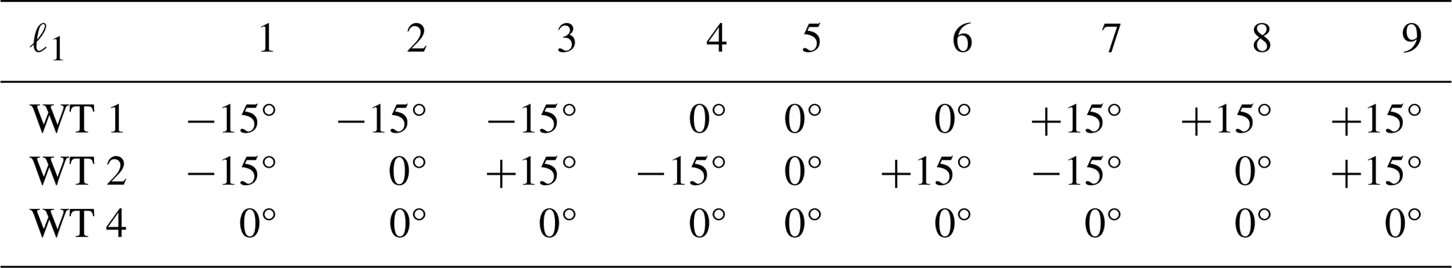
To illustrate the notions, we use Example in Sect. 2.1 (3×2 farm) again. For each covering section, marked in Fig. 5a, we need to uniquely identify every possible yaw configuration with an index, e.g., by sorting them lexicographically with respect to the yaw offsets (in increasing order of the turbine indices); Table 1 shows an example for covering section S₁, assuming for simplicity $\mathit{\{}-\mathrm{15}\mathit{°},\mathrm{0}\mathit{°},+\mathrm{15}\mathit{°}\mathit{\}}$ as admissible yaw offsets – the downstream-most turbines (4, 5, and 6) are fixed to 0°; cf. Sect. 1.2.1.

Table 1 Lexicographic indexing for $n_{\mathrm{\Delta },\mathrm{1}}={\mathrm{3}}^{\mathrm{2}}=\mathrm{9}$ yaw configurations for the underlying section configuration to covering section $S_{\mathrm{1}}=\mathit{\{}\mathrm{1},\mathrm{2},\mathrm{4}\mathit{\}}$ in the 3×2 farm Example in Sect. 2.1, cf. Fig. 5a, with simplified $\mathrm{\Gamma }=\mathit{\{}-\mathrm{15}\mathit{°},\mathrm{0}\mathit{°},+\mathrm{15}\mathit{°}\mathit{\}}$ (and WT 4 fixed to 0°).

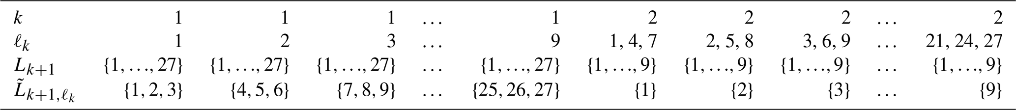
Assuming the same lexicographic indexing to the yaw configurations for each section configuration (and thus for the covering sections), we can determine the sets of valid yaw configurations; Table 2 shows the sets ${\stackrel{\mathrm{̃}}{L}}_{k+\mathrm{1},{\mathrm{\ell }}_k}$ for our simplified example. For instance, if yaw configuration ℓ₁=3 was used for S₁, then only the yaw configurations for S₂, in which turbines 1 and 2 also have yaw offsets −15° and +15°, respectively, are valid for S₂. With the indexing used, this amounts to ${\stackrel{\mathrm{̃}}{L}}_{\mathrm{2},\mathrm{3}}=\mathit{\{}\mathrm{7},\mathrm{8},\mathrm{9}\mathit{\}}$. For ℓ₂=7, only yaw configuration ℓ₃=1 is valid; indeed, ${\stackrel{\mathrm{̃}}{L}}_{\mathrm{3},\mathrm{7}}={\stackrel{\mathrm{̃}}{L}}_{\mathrm{3},\mathrm{1}}={\stackrel{\mathrm{̃}}{L}}_{\mathrm{3},\mathrm{4}}=\mathit{\left\{}\mathrm{1}\mathit{\right\}}$, as these yaw configurations for S₂ set both turbines 2 and 3 to −15°, for which the only compatible (and hence, valid) yaw configuration for S₃ is precisely ℓ₃=1.

Table 2 Valid yaw configurations ${\stackrel{\mathrm{̃}}{L}}_{k+\mathrm{1},{\mathrm{\ell }}_k}$ of covering section S_k+1 (depending on yaw configuration ℓ_k of the previous one S_k) compared to all possible yaw configurations L_k+1 of S_k+1 for the 3×2 farm from Example in Sect. 2.1, Fig. 5a, assuming admissible yaw offsets $\mathit{\{}-\mathrm{15}\mathit{°},\mathrm{0}\mathit{°},+\mathrm{15}\mathit{°}\mathit{\}}$ (simplified for the example) for every turbine, a fixed yaw offset of 0° for the downstream-most turbines, and yaw configurations that are indexed in lexicographical order. For S₁, all possible yaw configurations $L_{\mathrm{1}}=\mathit{\{}\mathrm{1},\mathrm{2},\mathrm{\dots },\mathrm{9}\mathit{\}}$ are also valid by design; i.e., ${\stackrel{\mathrm{̃}}{L}}_{\mathrm{1}}=L_{\mathrm{1}}$.

2.3.3 WFYP formulation as regular IP

Now, we introduce binary decision variables $y_{k,{\mathrm{\ell }}_k}$ that encode whether covering section S_k is assigned yaw configuration ℓ_k ($y_{k,{\mathrm{\ell }}_k}=\mathrm{1}$) or not ($y_{k,{\mathrm{\ell }}_k}=\mathrm{0}$). Using these variables, the black-box objective function, cf. Eq. (3), can be replaced by a fully linear one once we have precomputed the simulation results for the section configurations. Indeed, the simulation results allow us to specify cost coefficients $c_{k,{\mathrm{\ell }}_k}$ for every pair of a covering section S_k and any one of its associated yaw configurations ℓ_k; in order to avoid counting the objective contributions of turbines within intersecting parts of different covering sections multiple times, we again use a summation that only considers contributions of new turbines in a covering section (cf. Eq. 7):

$$\begin{array}{}\text{(8)}& c_{k,{\mathrm{\ell }}_k}:=\sum _{i\in T_k}{f}_{\mathit{\omega },i,j\left({\mathrm{\ell }}_k\right)}\left(x\right({\mathrm{\ell }}_k\left)\right).\end{array}$$

To achieve a globally optimal yaw configuration for the whole farm, we now have to optimize over all compatible combinations, see Sect. 2.3.2, of covering section and yaw configuration assignments (each of which has one associated coefficient $c_{k,{\mathrm{\ell }}_k}$ and one decision variable $y_{k,{\mathrm{\ell }}_k}$). This yields the following integer linear program to solve the WFYP:

$$\begin{array}{}\text{(9)}& \underset{y}{max}\sum _{k=\mathrm{1}}^{n_{\mathrm{s}}}\sum _{{\mathrm{\ell }}_k=\mathrm{1}}^{n_{\mathrm{\Delta },k}}{c}_{k,{\mathrm{\ell }}_k}{y}_{k,{\mathrm{\ell }}_k},\end{array}$$

$$\begin{array}{}\text{(10)}& \text{ s.t.}\sum _{{\mathrm{\ell }}_k=\mathrm{1}}^{n_{\mathrm{\Delta },k}}{y}_{k,{\mathrm{\ell }}_k}=\mathrm{1}\text{ for }k=\mathrm{1},\mathrm{\dots },n_{\mathrm{s}},\end{array}$$

$$\begin{array}{}\text{(11)}& \begin{array}{rl}& \mathrm{0}\le \sum _{{\mathrm{\ell }}_{k+\mathrm{1}}\in {\stackrel{\mathrm{̃}}{L}}_{k+\mathrm{1},{\mathrm{\ell }}_k}}{y}_{k+\mathrm{1},{\mathrm{\ell }}_{k+\mathrm{1}}}-y_{k,{\mathrm{\ell }}_k}\le \mathrm{1}\\ & \text{for}k=\mathrm{1},\mathrm{\dots },n_{\mathrm{s}}-\mathrm{1},{\mathrm{\ell }}_k=\mathrm{1},\mathrm{\dots },n_{\mathrm{\Delta },k},\end{array}\end{array}$$

$$\begin{array}{}\text{(12)}& \begin{array}{rl}{y}_{k,{\mathrm{\ell }}_k}\in & \mathit{\{}\mathrm{0},\mathrm{1}\mathit{\}}\\ & \text{ for }k=\mathrm{1},\mathrm{\dots },n_{\mathrm{s}},{\mathrm{\ell }}_k=\mathrm{1},\mathrm{\dots },n_{\mathrm{\Delta },k}.\end{array}\end{array}$$

Constraint (10) ensures that exactly one yaw configuration is selected for each covering section, analogously to Eq. (4). Constraint (11) ensures compatibility as it forces the selected yaw configuration for a covering section S_k+1 to be valid with respect to the yaw configuration chosen for its preceding covering section S_k, as described in Sect. 2.3.2: if $y_{k,{\mathrm{\ell }}_k}=\mathrm{1}$, i.e., S_k uses yaw configuration ℓ_k, then for S_k+1, a yaw configuration from ${\stackrel{\mathrm{̃}}{L}}_{k+\mathrm{1},{\mathrm{\ell }}_k}$ must be selected; i.e., one of the associated binary variables – and hence their sum – must be 1. If $y_{k,{\mathrm{\ell }}_k}=\mathrm{0}$, the constraint imposes no restriction¹ with respect to ${\stackrel{\mathrm{̃}}{L}}_{k+\mathrm{1},{\mathrm{\ell }}_k}$.

Finally, we emphasize that both black-box IP (3) to (5) and regular IP (9) to (12) are different formulations of the same problem, i.e., the WFYP; as such, they are equivalent – strictly speaking, this is only true if we take into account even the smallest wake-induced wind speed reduction to determine the upstream section instead of our practical assumption in Sect. 1.2.1. An example in Sect. 4 illustrates this small model inaccuracy. Nevertheless, the CA exploits the problem structure in a way that can significantly reduce the required number of simulations and enables the utilization of modern IP solvers to perform efficient implicit enumeration by branch and bound, thereby avoiding full enumeration.

3 Simulation

We obtain the simulation function output from simulation software that is interchangeable in our approach. Moreover, recall that our WFYP IPs (3) to (5) or (9) to (12) need simulation function values for different yaw offset configurations. As we control the yaw offsets, we only denote the corresponding decision variables x as simulation function arguments; the other inputs (farm layout, wind direction, and wind speed) are made clear in our experiments. In the following, we also introduce other conditions (and fixed values that we use) on which the simulation also depends.

3.1 Simulation software and parameter setup

For the farm simulations, we used the software package WinFaST.² This simulation framework requires a fixed farm layout. Axial induction and yaw offsets can be modified at any time during the simulation. As our focus lies on optimal yaw offsets, we leave the greedy control with respect to axial induction to the local controller. The dynamic wake model of WinFaST is based on FLORIDyn; see Gebraad and van Wingerden (2014). As FLORIDyn, it uses so-called observation points to compute local wake characteristics, and wake interaction is based on Katic et al. (1987). The turbine controller in WinFaST is inspired by Jonkman et al. (2009), which is widely used for NREL 5 MW turbines, and is extended by the options (not used by us) to reduce the power and/or damp tower oscillations, each with respect to its own respective turbine. Moreover, WinFaST uses a modified version (to include yaw control and effects) of the dynamic wind turbine model by Ritter et al. (2016, 2018). The wind field in WinFaST is simulated by the Veers method; see Veers (1988).

We denote the average wind speed value of the (horizontal) ambient wind field as U_ave. The TI is defined as $I=\mathit{\sigma }/U_{\mathrm{ave}}$, where σ is the associated standard deviation; it depends on the average wind speed, the roughness of the surface, the atmospheric stability, and the topography (see, e.g., Hau, 2013, their Sect. 13.4). WinFaST uses the same parametric model parameters for the turbine and wake as in Gebraad and van Wingerden (2014) (their Table 1), which are adjusted to 8 m s⁻¹ with a TI of 6 %, with the exception of the air density, which is set to 1.225 kg m⁻³, as in Jonkman et al. (2009) (their Appendix B.1). In our exemplary experiments, we fix the TI to 6 %.

3.2 Performance indicators and simulation function

It takes a while for the wake of the upstream-most turbine(s) to reach the downstream-most turbine within the upstream section. Thus, we need to choose a sufficiently long simulation time interval $[t_{{\mathrm{s}}_{\mathrm{1}}},t_{{\mathrm{s}}_{\mathrm{2}}}]$, depending on the wind speed, TI, and upstream section layout. Moreover, for data analysis and as yaw offsets are adjusted at a fairly low rate, we are only interested in the simulation part in which the wake already influences the downstream-most turbine. Moreover, the wind field is equipped with turbulence, and the turbines produce some turbulence as well, so we analyze data over an observation time interval $[t_{{\mathrm{o}}_{\mathrm{1}}},t_{{\mathrm{o}}_{\mathrm{2}}}]$; we use the data to compute the performance indicators and to define our simulation function. In practice, we round the minimal wind speed in the wind field down to 0.5 m s⁻¹ (namely, 4.5, 9, and 10 m s⁻¹ for speeds of 6, 11, and 12 with a TI of 6 %) and simulate with this speed and a TI of 0 % to round up the resulting propagation time in minutes to finally set a robust value for $t_{{\mathrm{o}}_{\mathrm{1}}}$; see Table 3 in Sect. 4 for examples. As we choose a duration of 10 min (to obtain roughly the specified wind speed on a mean at WT 3; cf. Table 3), we end up with $t_{{\mathrm{o}}_{\mathrm{2}}}=t_{{\mathrm{o}}_{\mathrm{1}}}+\mathrm{10}\min$ and $[t_{{\mathrm{s}}_{\mathrm{1}}},t_{{\mathrm{s}}_{\mathrm{2}}}]=[\mathrm{0},t_{{\mathrm{o}}_{\mathrm{2}}}]$.

The performance indicators (cf. Eq. 14 later) consist of the following three outputs of WinFaST: the power generated by each turbine is given in units of watts as function $p_x:[t_{{\mathrm{s}}_{\mathrm{1}}},t_{{\mathrm{s}}_{\mathrm{2}}}]\to {\mathbb{R}}_{\ge \mathrm{0}}^{n_{\mathrm{WT}}}$. To compute loads we use the velocity of the nacelle in meters per second in the wind direction, $v_x:[t_{{\mathrm{s}}_{\mathrm{1}}},t_{{\mathrm{s}}_{\mathrm{2}}}]\to {\mathbb{R}}^{n_{\mathrm{WT}}}$, and the blade pitch angle in the unit degree, ${\mathit{\beta }}_x:[t_{{\mathrm{s}}_{\mathrm{1}}},t_{{\mathrm{s}}_{\mathrm{2}}}]\to {\mathbb{R}}^{n_{\mathrm{WT}}}$.

Now, we define the three performance indicators for each turbine i as averages over the observation time interval $[t_{{\mathrm{o}}_{\mathrm{1}}},t_{{\mathrm{o}}_{\mathrm{2}}}]$, namely the power (output) P_i (in MW), the tower activity $a_i^{\left(\mathrm{T}\right)}$, and the pitch activity $a_i^{\left(\mathrm{P}\right)}$. The tower load is high when the nacelle oscillates; therefore, we use the absolute value of the nacelle velocity v to estimate the tower load through the so-called tower activity. The pitch rate should be kept within limits because of the load of the pitch actuators; therefore, similarly, we use the absolute value of the velocity of the blade pitch angle β to estimate the load of the pitch actuators using the so-called pitch activity. The performance indicators are defined as follows:

$$\begin{array}{}\text{(13)}& \begin{array}{rl}{P}_i\left(x\right)& :={\displaystyle \frac{\mathrm{1}}{t_{{\mathrm{o}}_{\mathrm{2}}}-t_{{\mathrm{o}}_{\mathrm{1}}}}}\underset{t_{{\mathrm{o}}_{\mathrm{1}}}}{\overset{t_{{\mathrm{o}}_{\mathrm{2}}}}{\int }}{\mathrm{10}}^{-\mathrm{6}}\left(p_x\right(t){)}_i\mathrm{d}t,\\ a_i^{\left(\mathrm{T}\right)}\left(x\right)& :={\displaystyle \frac{\mathrm{1}}{t_{{\mathrm{o}}_{\mathrm{2}}}-t_{{\mathrm{o}}_{\mathrm{1}}}}}\underset{t_{{\mathrm{o}}_{\mathrm{1}}}}{\overset{t_{{\mathrm{o}}_{\mathrm{2}}}}{\int }}\left|\left(v_x\right(t){)}_i\right|\mathrm{d}t,\\ a_i^{\left(\mathrm{P}\right)}\left(x\right)& :={\displaystyle \frac{\mathrm{1}}{t_{{\mathrm{o}}_{\mathrm{2}}}-t_{{\mathrm{o}}_{\mathrm{1}}}}}\underset{t_{{\mathrm{o}}_{\mathrm{1}}}}{\overset{t_{{\mathrm{o}}_{\mathrm{2}}}}{\int }}\left|{\displaystyle \frac{\mathrm{d}}{\mathrm{d}t}}\left({\mathit{\beta }}_x\right(t){)}_i\right|\mathrm{d}t.\end{array}\end{array}$$

The respective units of tower and pitch activity are m s⁻¹ and ° s⁻¹ but have no physical meaning.

Finally, we define the weighted sum of these three performance indicators as the simulation function depending on the control input, i.e., the decision variables x. Recall that the dependence on yaw configurations also includes the dependence of a turbine i∈T on its own yaw offset, which can be expressed using the yaw offset index $j\in n_{\mathrm{\Gamma },i}$. Therefore, following the notation introduced in Sect. 2.1, we write P_i,j(x), $a_{i,j}^{\left(\mathrm{T}\right)}\left(x\right)$, and $a_{i,j}^{\left(\mathrm{P}\right)}\left(x\right)$. With weights $\mathit{\omega }=({\mathit{\omega }}^{\left(\mathrm{T}\right)},{\mathit{\omega }}^{\left(\mathrm{P}\right)})\in {\mathbb{R}}_{\ge \mathrm{0}}^{\mathrm{2}}$ for the activity terms, the entries of the simulation function, which yields the black-box function to be maximized, are

$$\begin{array}{}\text{(14)}& f_{\mathit{\omega },i,j}\left(x\right):=P_{i,j}\left(x\right)-{\mathit{\omega }}^{\left(\mathrm{T}\right)}{a}_{i,j}^{\left(\mathrm{T}\right)}\left(x\right)-{\mathit{\omega }}^{\left(\mathrm{P}\right)}{a}_{i,j}^{\left(\mathrm{P}\right)}\left(x\right).\end{array}$$

It represents our two main objectives when controlling the farm: maximizing the total power output and minimizing the turbines' mechanical load; the weights balance these typically conflicting objectives. In fact, they could even do this individually for each turbine. Moreover, for simplicity, we focus on the power output; i.e., usually ${\mathit{\omega }}^{\left(\mathrm{T}\right)}={\mathit{\omega }}^{\left(\mathrm{P}\right)}=\mathrm{0}$ in Sect. 4. In practice, one simulation run consists of evaluating the (vector-valued) simulation function $f_{\mathit{\omega }}:\mathit{\{}\mathrm{0},\mathrm{1}{\mathit{\}}}^{n_{\mathrm{\Gamma },\mathrm{1}}+\mathrm{\dots }+n_{\mathrm{\Gamma },n_{\mathrm{WT}}}}\to {\mathbb{R}}^{n_{\mathrm{WT}}}$ (with entries of the form $f_{\mathit{\omega },i,j}\left(x\right)$) once for the associated section and assignment of decision variables x.

4 Computational results

In order to obtain computational results, we show the overall process in Fig. 6 as it is a combination of CA (see Sect. 2.2), its formulation as IP (see Sect. 2.3), and simulation (see Sect. 3).

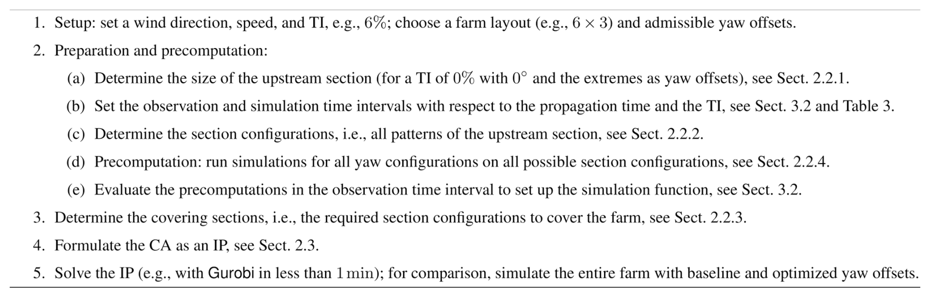
Figure 6 Overall process to obtain computational results (as a combination of CA, IP formulation, and simulation).

All computations were carried out on a Linux workstation with an Intel^® Core™ i7-6700 CPU with 3.40 GHz (four cores, eight threads) and 32 GB memory. The precomputations (simulation runs) were done using MATLAB R2024b, utilizing parallelization of four workers. The IPs resulting from our CA were solved with state-of-the-art IP solvers, namely the open-sourced academic solver SCIP 8.0.3, utilizing the LP solver SoPlex 6.0.3, which only supports single threads (see Bestuzheva et al., 2021), and the proprietary Gurobi 10.0.0, which can employ all threads (see Gurobi Optimization, 2022).

Before we discuss the results, we briefly summarize the most important parts of the overall experimental setup. As admissible yaw offsets we choose $\mathit{\gamma }\in \mathrm{\Gamma }=\mathit{\{}-\mathrm{15}\mathit{°},-\mathrm{10}\mathit{°},\mathrm{\dots },\mathrm{15}\mathit{°}\mathit{\}}$ for NREL 5 MW turbines with a rotor diameter of D=126 m, see Jonkman et al. (2009) (their Table 1-1), in different farm layouts from 6×3 to 9×3 with a turbine spacing of 3D×5D. As wind directions we use 0, 5, 10, or 20°, where 0° represents wind blowing from west to east. In all figures, we indicate the wind direction by a vector. As average wind speeds we consider 6, 11, and 12 m s⁻¹. Deviations from this setup are made clear where they occur. Finally, we frequently compare the optimized yaw offsets against the baseline, i.e., yaw offsets of 0°.

The main computational experiments in a farm with our CA are in Sect. 4.1 to 4.4: for different wind directions, reused precomputed simulations to demonstrate flexibility, different wind speeds, and different yaw offset discretizations. However, we begin with some experiments to compare the WinFaST simulation with the FLORIS software, see NREL (2024), and continue with a comparison of our CA on the basis of the simulation software FLORIS with the serial-refine (SR) method (available in FLORIS), see Fleming et al. (2022), and full enumeration (as assumptions and discretizations were employed to arrive at our IP model for the WFYP via the CA).

To that end, we consider a 3×3 farm with different TIs, wind speeds, and wind directions and compare the baseline simulations of WinFaST and FLORIS in Table 3; see Fig. 7a for a visualization of part (c). Specifically, we use the available file gch.yaml as input in FLORIS, i.e., the sophisticated static Gauss–curl hybrid wake model, but set the wind shear to 0. While the results are similar at WT 3, they differ significantly at WTs 5 and 7 as WinFaST generates a wind field and uses dynamic turbine and wake models. Simulation is a complex topic; e.g., WinFaST simulates a scenario in which WT 3 sometimes reaches 5 MW due to turbulence in parts (c) to (f). An extensive comparison of the simulations (and which one is preferable) is out of the scope of the present paper.

For the mentioned CA comparison on the basis of the FLORIS software simulation, we consider a 3×3 farm with a wind speed of 11 m s⁻¹ (TI of 6 %). As our CA is equivalent to full enumeration for sufficiently large upstream sections, see Sect. 2.3.3, it achieves the same or greater total power output compared to the fast SR method. To demonstrate this advantage, we have to extend the range of admissible yaw offsets and exceptionally use $[-\mathrm{20}\mathit{°},+\mathrm{20}\mathit{°}]$ in 10° steps; i.e., in the SR method, we use three yaw offsets in the first phase (i.e., 20° steps) and two in the second phase. For wind directions of $\mathrm{0},\mathrm{5},\mathrm{\dots },\mathrm{45}\mathit{°}$, our CA always results in the same total power outputs as the full enumeration, whereas in three cases, the SR method results in slightly lower ones (between 0.5 % and 0.8 %). The run times are between 3 s and 7 min with full enumeration, between 2 s and 11 s with CA, and always 1 s with SR method, which is not directly comparable as we designed the CA with flexibility in mind; see Sect. 2.2.2. The case with a wind direction of 20°, i.e., in which the controlled WTs are 2, 3, 5, and 6 (cf. the assumptions in Sect. 1.2.1), is in Table 4 from α to γ. For the same case but with our default yaw offset discretization, i.e., $[-\mathrm{15}\mathit{°},+\mathrm{15}\mathit{°}]$ in 5° steps, which we use from now on, we refer to Table 4a to c and Fig. 7. Specifically, full enumeration takes 82 s and results in four solutions with an optimized total power output of 38.66 MW. Our CA takes 18 s and predicts a power of 38.69 MW, but the full farm simulation with optimal yaw offsets also results in 38.66 MW. For the SR method, we allow seven yaw offsets in the first phase, i.e., our usual choice of 5° steps, and two in the second phase, which practically corresponds to finer steps of 2.5°, which is actually used for WTs 2 and 5 and results in an improved total power output of 38.68 MW after a run time of 1 s. Finally, we have to find out under which conditions our CA is worthwhile compared to the SR method, but this is out of the scope of the present paper.

The deviations in the predicted power by the CA and full farm simulation (in baseline and/or optimization) are limited and are due to the size of the upstream section, which influences the accuracy of the discretized, section-based WFYP model and therefore is a compromise in terms of accuracy and run time. For example, the covering section (based on upstream section Fig. 3d) anchored at WT 4 includes WT 2, but WT 1 is marginally outside. An increase in the size of the upstream section would ameliorate the small model inaccuracy but also significantly increase the precomputation time. Therefore, we accept small inaccuracies in the predicted power output by CA (and run a full simulation with optimized yaw offsets at the end). As the improvements over the baseline are significantly larger than the deviations from the full farm simulation, the optimal solutions of our CA will likely still be optimal for a model using increased upstream sections, though suboptimality is technically possible. The IP solver run times themselves will indicate that handling larger upstream sections should not pose an issue.

For the remainder of the paper, we show the results of our CA approach using the WinFaST simulation for computations and visualize the results with FLORIS software. For the example above, we receive other optimized yaw offsets, see Table 4d and Fig. 7b, where the precomputation takes 4.5 h and the IP solver SCIP 0.11 s. These yaw offsets as input in FLORIS result in 38.27 MW, which is below the baseline with FLORIS and demonstrates the dependency of the solution on the selected simulation. In addition, we use the introduced weights $\mathit{\omega }=({\mathit{\omega }}^{\left(\mathrm{T}\right)},{\mathit{\omega }}^{\left(\mathrm{P}\right)})=(\mathrm{100},\mathrm{10})$ once to take into account the tower activity and pitch activity in optimization (cf. Eq. 14 and see Table 4e). A detailed comparison to (d) using our default $\mathit{\omega }=(\mathrm{0},\mathrm{0})$ shows that both tower and pitch activities are reduced to 0.1105 (from 0.1108) and 0.3865 (0.4070) at the cost of a power reduction (to 33.03 from 33.05 MW). For reference, the baseline tower and pitch activity values are 0.1128 and 0.5347.

Table 3 Data and results for baseline simulations of a 3×3 farm to compare WinFaST and FLORIS (series 0, case 0). Both the observation time interval $[t_{{\mathrm{o}}_{\mathrm{1}}},t_{{\mathrm{o}}_{\mathrm{2}}}]$ and the mean wind speed at WT 3 are related to WinFaST; we set $t_{{\mathrm{o}}_{\mathrm{1}}}$ and $t_{{\mathrm{o}}_{\mathrm{2}}}=t_{{\mathrm{o}}_{\mathrm{1}}}+\mathrm{10}\min$, as discussed in Sect. 3.2.

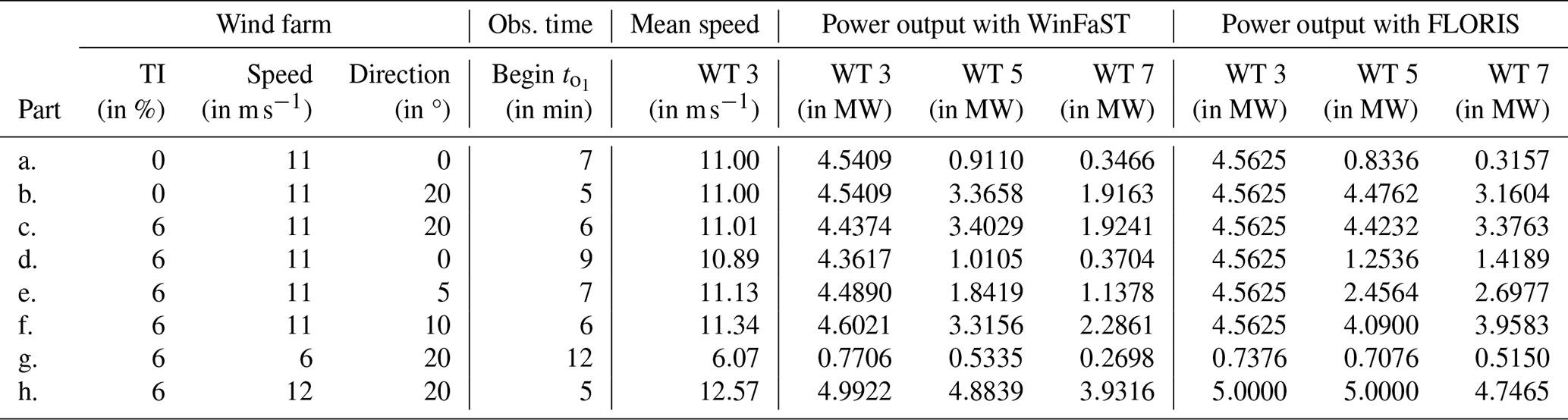
Table 4 Data and results for a 3×3 farm, a wind speed of 11 m s⁻¹ (TI of 6 %), and a direction of 20° (series 0, case 1) to compare optimization methods and simulations. In cases of CA we add the run times of precomputations and the IP solver SCIP. In parts (α) to (γ), the yaw offset discretization is exceptionally $[-\mathrm{20}\mathit{°},\mathrm{20}\mathit{°}]$ in 10° steps (instead of $[-\mathrm{15}\mathit{°},\mathrm{15}\mathit{°}]$ in 5° steps), and in (b) we practically allow 2.5° steps. In part (e) we take into account the tower activity (weighted by 100) and the pitch activity (weighted by 10); cf. Eq. 14 (marked with “(w)”).

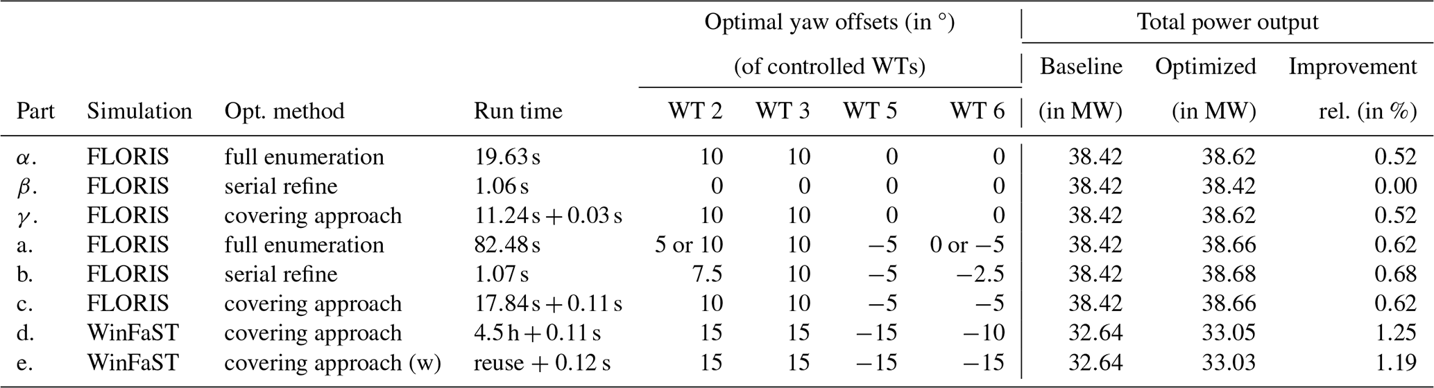
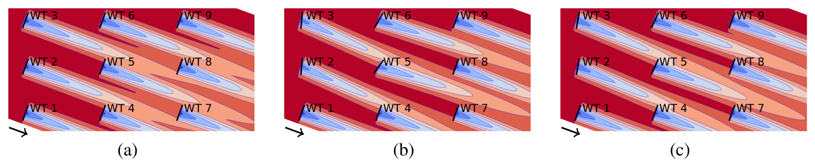
Figure 7 Baseline and optimization results for comparison (visualized with FLORIS). In the following, we compare the farm's power output. (a) Baseline: 32.64 MW with WinFaST, 38.42 MW with FLORIS. (b) Optimized with covering approach with WinFaST: 33.05 MW. (c) Optimized with covering approach with FLORIS: 38.66 MW.

4.1 Wind farm yaw offset optimization under different wind directions

In series 1, we consider a 6×3 farm with a wind speed of 11 m s⁻¹ and wind directions of 0, 5, 10, and 20°. The respective results are presented in Table 5; see also Fig. 9b for case 4. In all cases, the improvement in the total power output is between 2 % and 17 %. In most of these cases, the optimal yaw offsets exhaust the given limits of ±15°. In case 4 (i.e., wind direction of 20°), the distances between the turbines in the downstream direction are already comparatively high, and, consequently, the wake influence is comparatively low; therefore, the improvement is 2 % here but larger in the other cases.

Table 5 Data and results for a 6×3 farm; a wind speed of 11 m s⁻¹; and wind directions of 0, 5, 10, and 20° (series 1). In all cases, the IP optimality gap is 0.00 %; i.e., all instances were solved to global optimality. Detailed results of case 4 are in Fig. 9b.

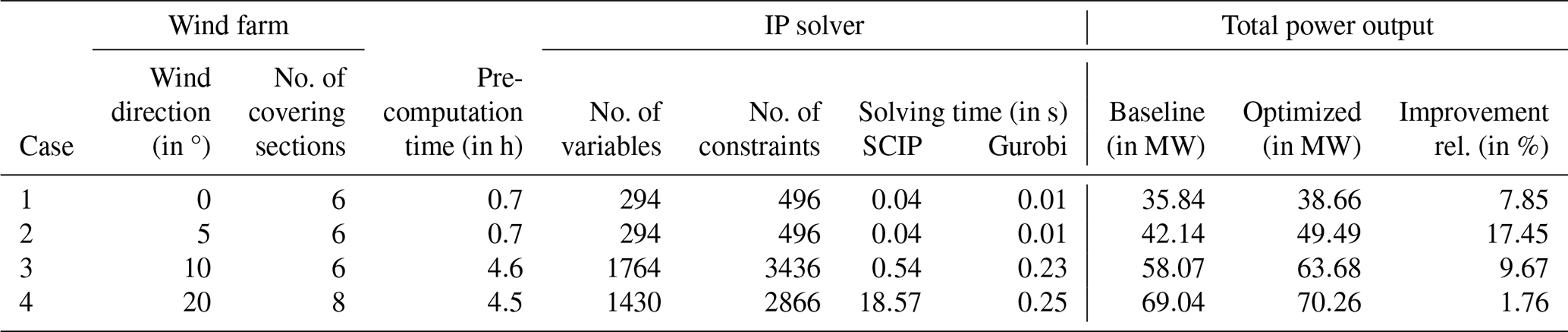
The main part of the overall run time is the precomputation time; e.g., in series 1 it is about 1 to 5 h. The IPs in our CA are then all solved in well below 1 s by Gurobi and still within at most 19 s by SCIP. We remind the reader that the precomputations were designed with flexibility in mind (see Sect. 2.2.2); i.e., they can be reused for many cases (see our series 2 for a demonstration). Hence, for the actual optimization process used for control updates, only the IP solving times are relevant, which turned out to be so small that we can regard the optimization as capable of real-time application (cf. Sect. 1.2.2). Finally, we see that the suggested database of precomputed simulation results, see Sect. 2.2.4, is time-consuming to build but enables significant gains through optimization.

The main influence on the precomputation time is the turbines' number in the upstream section; the impact of the allowed number of yaw offsets is smaller (cf. Sect. 4.4). The specific upstream sections in series 1 are depicted in Fig. 3; those of cases 1 and 2 (i.e., wind directions 0 and 5°) include three turbines and yield precomputation times of about an hour (cf. Table 5), whereas those of cases 3 and 4 (i.e., 10 and 20°) include four turbines and take about 5 h. Four turbines (with seven possible yaw offsets) result in 512 yaw configurations (i.e., simulations); see Example in Sect. 2.2 and Eq. (6).

4.2 Scalability and flexibility of the covering approach to solve the WFYP

In series 2, we demonstrate that reusing precomputed simulation results (for section configurations, see Sect. 2.2), namely series 1, case 4 (case 1.4), see Table 5, enables our CA to enlarge farms orthogonal to the wind direction (cases 2.1 to 2.4) and to handle cases with deactivated turbines (case 2.5). In particular, we use a wind direction of 20° and a speed of 11 m s⁻¹ to reuse case 1.4 precomputations (originally for a 6×3 farm) for 7×3 to 9×3 and monitor the IP solvers' workload; see Table 6. The optimization consistently improves the farm's total power output by roughly 2 %. The impact of the farm size on the IP solving time reflects the theoretical complexity of the WFYP (see Prop. in Sect. 2.1) in practice: the solver SCIP quickly takes a long time – it could be stopped earlier if a duality gap was accepted; Gurobi is faster by orders of magnitude, remaining well below 1 min in all cases considered here, despite an (apparently exponential) increase in run time with the farm size. This illustrates the practical scalability of our CA and, in light of the low yaw sampling rate, its suitability for real-time WFYP optimization – even for farms with more turbines than those explored here. Moreover, we demonstrate the curse of dimensionality of full enumeration via predicted run times, namely of the order of 10² to 10⁸ years, instead of the 4.5 h precomputation (cf. Table 5).

Furthermore, we handle case 2.5 with a mix of active and inactive (or non-existing) turbines to show our method's practical flexibility, e.g., in response to a shutdown for maintenance. Again, we reuse precomputations of case 1.4, cf. Table 5, but now in the setting depicted in Fig. 8; i.e., WTs $\mathit{\{}\mathrm{2},\mathrm{5},\mathrm{6},\mathrm{9},\mathrm{12}\mathit{\}}$ are inactive. The WFYP optimization still yields an improvement of about 2 % in generated power, namely 1.95 %, while the “thinning out” of the farm leads to notably shorter IP solving times: 0.02 s (instead of 18.57 s) with SCIP and below 0.01 s (0.25 s) using Gurobi.

Table 6 Data and results used to illustrate the scalability and complexity of the WFYP (series 2). All cases have a wind direction of 20° and a speed of 11 m s⁻¹. In all cases, the IP optimality gap is 0.00 %. (Case 2.1 repeats case 1.4.) We estimate the predicted run time of full enumeration through $n_{\mathrm{\Gamma }}^{n_{\mathrm{WT}}-n_{\mathrm{s}}}\cdot \mathit{\tau }\cdot \mathrm{1}/\mathrm{4}$, where τ is the run time of one simulation and $\mathrm{1}/\mathrm{4}$ is for the parallelization effect; see Sect. 2.2.4 for a number of combinations.

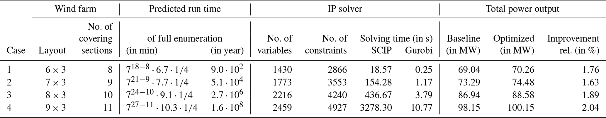
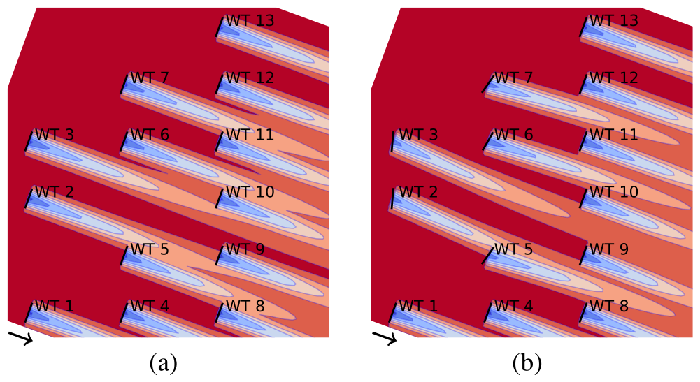
Figure 8 Detailed results for a 6×3 farm in which some turbines are inactive (case 2.5 with a wind speed of 11 m s⁻¹ and direction of 20°). The total power outputs of the farm are (a) 54.51 MW with baseline yaw offsets and (b) 55.57 MW with optimized ones.

4.3 Impact of different wind speeds

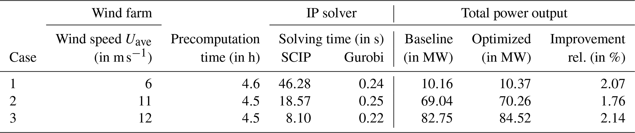
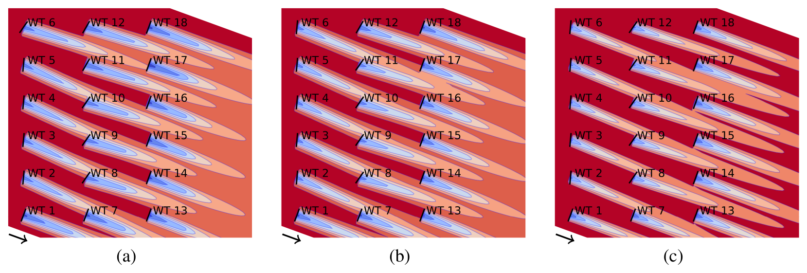
In series 3, we again consider a 6×3 farm and a wind direction of 20° and evaluate WFYP solutions for different wind speeds. The baseline and optimization results of 6, 11, and 12 m s⁻¹ are reported in Table 7 (11 m s⁻¹ repeats case 1.4) and Fig. 9: the optimization increases the farm's total power output by about 2 %; the maximum of the precomputation time is about 5 h and about 46 s (SCIP) or under 1 s (Gurobi) for the IP solving time. Finally, further experiments provide speeds of $\mathit{\{}\mathrm{6},\mathrm{7},\mathrm{\dots },\mathrm{15}\mathit{\}}\mathrm{m}{\mathrm{s}}^{-\mathrm{1}}$: the improvement in the total power is between 0.90 % and 2.54 % for 6 to 13 m s⁻¹, 0.06 % for 14 m s⁻¹, and 0.00 % for 15 m s⁻¹ (as the baseline already reaches the maximum of 90 MW). For 6 to 14 m s⁻¹ we obtain yaw offsets of the controlled WTs with a similar power output effect, namely ±15° for WTs 2 to 6 and −10° or −15° for WTs 8 to 12. This suggests several approaches: the avoidance of many precomputations by identifying the wind speeds' “tipping points” for each wind direction, i.e., speeds that change the optimal yaw offsets (significantly with regard to the total power), the restriction of admissible yaw offsets around the found values, or the refinement of yaw offsets around the found values (similar to the SR method; see Fleming et al., 2022). Further, we observe that turbines in a row (apart from those at the farm borders) appear to typically have identical optimal yaw offsets (in the same experiment). This is likely due to the grid layout, whereby, on the one hand, we also have to acknowledge that our number of admissible yaw offsets is not large, and, on the other hand, we refer to Sect. 4.4 for the effects and usefulness of a finer discretization. In addition, the optimal yaw offsets of all controlled WTs differ from 0°: on the one hand, this may provide opportunities to reduce the running times of both precomputations and IP solving, and, on the other hand, it might be different for other wind directions, although there are already relatively few wake interactions for the wind direction of 20° (which is reflected in the relatively small potential for total power improvement). Finally, the speed of 15 m s⁻¹ is the end of interest from a total power optimization perspective for the present example, as the improvement is 0.00 %. Nevertheless, optimization can still be meaningful if mechanical loads are included: in a further experiment, we weight the tower activity by ω^(T)=100 and the pitch activity by ω^(P); cf. Eq. (14). This results in optimal yaw offsets that are similar to those for 6 to 14 m s⁻¹, namely ±15° for WTs $\mathit{\{}\mathrm{2},\mathrm{\dots },\mathrm{5},\mathrm{8},\mathrm{\dots },\mathrm{12}\mathit{\}}$ and 10° for WT 6. The total power remains at 90 MW, whereas the tower activity decreases to 0.4017 (from 0.4096 in baseline), but the less heavily weighted pitch activity increases to 4.2175 (from 4.1707).

Table 7 Data and results used to illustrate the impact of wind speeds (series 3). All cases have a 6×3 farm layout and a wind direction of 20° in common. In all cases, the IP optimality gap is 0.00 %. Detailed results are in Fig. 9. (Case 3.2 repeats case 1.4.)

Figure 9 Optimization results for series 3, as shown in Table 7. The optimized farm's total power outputs are (a) 10.37 MW for a wind speed of 6 m s⁻¹, (b) 70.26 MW for 11 m s⁻¹, and (c) 84.52 MW for 12 m s⁻¹.

4.4 Modifying the yaw offset discretization in terms of range and fineness

In series 4, we deviate from the yaw offset discretization ($[-\mathrm{15}\mathit{°},\mathrm{15}\mathit{°}]$ in 5° steps, i.e., seven offsets) used so far; see Table 8 for the results. In case 4.1, we use $[-\mathrm{40}\mathit{°},\mathrm{40}\mathit{°}]$ in 5° steps, i.e., 17 offsets, for the setup as in case 1.2 (with which we compare; cf. Table 5). This increases the precomputation time to 2.6 h (compared to 0.7 h). As an optimal result, all controlled turbines are set to 30°, which enables a significantly increased power output of the downstream-most turbines (with 0°), i.e., 2.9 to 3.1 MW (from 1.7 to 1.9 MW). The total farm output is increased to 53.81 MW (from 49.49 MW). The non-use of the new limits of ± 40° shows that at the extreme yaw offset settings, the power loss at a turbine would exceed the gain at turbines downstream.

In case 4.2, we reconsider $[-\mathrm{15}\mathit{°},\mathrm{15}\mathit{°}]$ but with 2.5° steps, i.e., 13 offsets, for the setup as in case 1.4 (with which we compare; cf. Table 5), which is particularly interesting for finer discretization as not all turbines attain extreme yaw offsets of ±15°. Indeed, optimal yaw offsets of WTs 8 to 12 are set to −12.5° (from −15° or −10° for WT 12), whereas WTs 2 to 6 remain at 15° (and others at 0°). The longer precomputation time of 23.0 h (4.5 h) is theoretically worthwhile as the total power output is increased further to 70.29 MW (from 70.26 MW). In practice, it is unnecessary to use arbitrarily fine discretizations due to the uncertainty in incident wind conditions; see Stanley et al. (2022) (referenced in Sect. 1.2.1).

Table 8 Data and results if yaw offset range or discretization is changed (series 4). All cases consider a 6×3 farm with a wind speed of 11 m s⁻¹. In all cases, the IP optimality gap is 0.00 %.

5 Concluding remarks

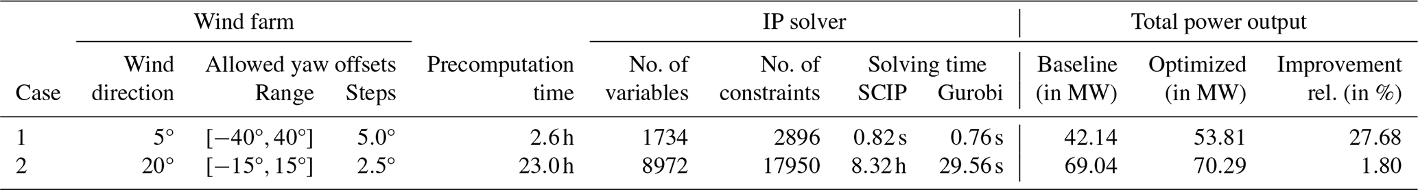
We formulated the wind farm yaw problem mathematically, established its computational complexity, and developed a covering approach that makes use of repeating patterns (based on the so-called upstream section) to cover the wind farm in the form of integer programming to solve it faster. Building on a number of simulation results that can be precomputed at any time before the need for farm-level yaw control arises, the method is efficient in practice in spite of the problem's strong 𝒩𝒫 hardness and inapproximability. In particular, we fully expect even very long precomputation times (e.g., months) to be acceptable as the simulations can easily be run for various wind scenarios while the farm is not yet operational. Given the envisioned database, our CA efficiently delivers optimal farm-level yaw control using a state-of-the-art IP solver like Gurobi. The solution is even globally optimal under some mild assumptions, as discussed in Sect. 1.2.1, including discretized yaw offsets, the chosen size of the so-called upstream section, and a homogeneous layout structure. We demonstrated this through a comparison with full enumeration, in which we interchanged the simulation on which our superordinate model is based with FLORIS software (which does not utilize dynamic models for wakes and turbines). In addition, our CA makes it possible to address wind farms with many turbines. We demonstrated the performance of our approach with several proof-of-concept examples that illustrate its effectiveness, flexibility, and scalability, particularly through the reuse of precomputations if we enlarge the farm orthogonally to the wind direction or deactivate turbines. On the other hand, the enlargement in the wind direction increases the upstream section and therefore the number of turbines inside, which mainly increases the precomputation time. Finally, solving the WFYP for several farms using our CA for a variety of wind directions and speeds should be helpful to recognize structures whose exploitation reduces the computational effort in precomputation or simplifies the WFYP itself.

Appendix A: Complexity of the wind farm yaw problem

This section addresses the computational complexity of the wind farm yaw problem from a theoretical viewpoint; we assume basic knowledge of mathematical complexity theory and refer to Garey and Johnson (1979) for a detailed introduction. Using the basic black-box IP formulation (3) to (5) of the WFYP (cf. Sect. 2.1), we show that the WFYP is strongly 𝒩𝒫 hard (Theorem A4) and even hard to approximate (Corollary A6). These two results together yield Proposition in Sect. 2.1. We use the well-known strongly 𝒩𝒫-complete Hamiltonian circuit (HC) problem; see, e.g., Garey and Johnson (1979) (problem GT37), for our proof.

A1 Definition

Hamiltonian circuit problem (HCP). Let an undirected graph $G=(V,E)$ on n vertices, $V:=\mathit{\{}{v}_{\mathrm{1}},\mathrm{\dots },v_n\mathit{\}}$, be given. Does G contain a Hamiltonian circuit, i.e., a subset of edges $\mathcal{H}=\left\{\mathit{\{}{v}_{\mathit{\pi }\left(\mathrm{1}\right)},v_{\mathit{\pi }\left(\mathrm{2}\right)}\mathit{\}},\mathit{\{}{v}_{\mathit{\pi }\left(\mathrm{2}\right)},v_{\mathit{\pi }\left(\mathrm{3}\right)}\mathit{\}},\mathrm{\dots },\mathit{\{}{v}_{\mathit{\pi }(n-\mathrm{1})},v_{\mathit{\pi }\left(n\right)}\mathit{\}},\right.$ $\left.\mathit{\{}{v}_{\mathit{\pi }\left(n\right)},v_{\mathit{\pi }\left(\mathrm{1}\right)}\mathit{\}}\right\}\subset E$ for a permutation $\langle v_{\mathit{\pi }\left(\mathrm{1}\right)},v_{\mathit{\pi }\left(\mathrm{2}\right)},\mathrm{\dots },v_{\mathit{\pi }\left(n\right)}\rangle$ of V?

For clarity, we also explicitly state the decision version of the WFYP problem.

A2 Definition

WFYP decision version (WFYP-DEC). Let the index set T of wind turbines in a farm, its layout ℒ, the index set ${\mathrm{\Gamma }}_i:=\mathit{\{}\mathrm{1},\mathrm{\dots },n_{\mathrm{\Gamma },i}\mathit{\}}$ of admissible yaw offsets for each turbine i∈T, the WFYP objective function $f_{\mathit{\omega }}^{\mathrm{\Sigma }}$ as defined for its (black-box) IP formulation, and a number F∈ℝ be given. Does a feasible yaw configuration for the given farm (i.e., exactly one yaw offset per turbine) exist such that, for the associated binary yaw offset assignment vector x, $f_{\mathit{\omega }}^{\mathrm{\Sigma }}\left(x\right)\ge F$?

A3 Remark

Recall that the assignment vector $x\in \mathit{\{}\mathrm{0},\mathrm{1}{\mathit{\}}}^{{n_{\mathrm{\Gamma }}}_{\mathrm{1}}+\mathrm{\dots }+{n_{\mathrm{\Gamma }}}_{n_{\mathrm{WT}}}}$, with the entry in position ${\sum }_{\mathrm{\ell }=\mathrm{1}}^{i-\mathrm{1}}{n_{\mathrm{\Gamma }}}_{\mathrm{\ell }}+j$ being denoted by x_i,j and having a value of 1 if and only if the ith turbine is set to the jth yaw offset from among the respective admissible set Γ_i. In the following, we also use additional notation: we denote the so-called triangular numbers as ${\mathrm{\Delta }}_n:=\left(\genfrac{}{}{0ex}{}{n+\mathrm{1}}{\mathrm{2}}\right)=\frac{n^{\mathrm{2}}+n}{\mathrm{2}}$, abbreviate the set of the first N triangular numbers as $\mathrm{\Delta }\left(N\right):=\mathit{\{}{\mathrm{\Delta }}_{\mathrm{1}},{\mathrm{\Delta }}_{\mathrm{2}},\mathrm{\dots },{\mathrm{\Delta }}_N\mathit{\}}$, and write $\left[n\right]:=\mathit{\{}\mathrm{1},\mathrm{2},\mathrm{\dots },n\mathit{\}}$ for n∈ℕ.

We are now prepared to prove the 𝒩𝒫 hardness and inapproximability of the WFYP(-DEC).

A4 Theorem

The WFYP is strongly 𝒩𝒫 hard.

Proof. We show hardness for the decision version WFYP-DEC, which directly implies hardness for the optimization version (WFYP, as defined in Sect. 2); cf. Garey and Johnson (1979). To that end, we reduce from the strongly 𝒩𝒫-complete HCP.

Let $G=(V,E)$ be an arbitrary HCP instance and denote $n=\left|V\right|$. We can assume without loss of generality that n≥2, every vertex has a degree of at least 2, and G consists of a single connected component (otherwise, the answer to the HCP is trivially “no”). We construct an instance $(T,\mathcal{L},\mathit{\{}{\mathrm{\Gamma }}_i{\mathit{\}}}_{i\in T},f_{\mathit{\omega }}^{\mathrm{\Sigma }},F)$ of the WFYP-DEC as follows.

We set the number of turbines to $n_{\mathrm{WT}}:={\mathrm{\Delta }}_n+\mathrm{1}$ and identify the turbines by their index; i.e., $T:=[{\mathrm{\Delta }}_n+\mathrm{1}]$. The turbines are arranged in a triangle-like layout ℒ (on a regular grid)³ defined by the following “row” sets:

$$\begin{array}{}\text{(A1)}& \begin{array}{rl}& R_{\mathrm{1}}:=\mathit{\left\{}{\mathrm{\Delta }}_{\mathrm{1}}\mathit{\right\}}=\mathit{\left\{}\mathrm{1}\mathit{\right\}},R_{\mathrm{2}}:=\mathit{\{}{\mathrm{\Delta }}_{\mathrm{2}},\mathrm{2}\mathit{\}},R_{\mathrm{3}}:=\mathit{\{}{\mathrm{\Delta }}_{\mathrm{3}},\mathrm{5},\mathrm{4}\mathit{\}},\\ & \mathrm{\dots },R_n:=\mathit{\{}{\mathrm{\Delta }}_n,{\mathrm{\Delta }}_n-\mathrm{1},\mathrm{\dots },{\mathrm{\Delta }}_{n-\mathrm{1}}+\mathrm{1}\mathit{\}},\\ & R_{n+\mathrm{1}}:=\mathit{\{}{\mathrm{\Delta }}_n+\mathrm{1}\mathit{\}}.\end{array}\end{array}$$

Furthermore, each turbine i∈T is given the same set of admissible yaw offsets ${\mathrm{\Gamma }}_i:=\mathrm{\Gamma }:=\left[n\right]$, so $n_{\mathrm{\Gamma },i}=\left|{\mathrm{\Gamma }}_i\right|=n$ for all i∈T. Finally, we set F:=n and define the terms $f_{\mathit{\omega },i,j}\left(x\right)$ of the simulation function $f_{\mathit{\omega }}^{\mathrm{\Sigma }}\left(x\right):={\sum }_{i=\mathrm{1}}^{n_{\mathrm{WT}}}{\sum }_{j=\mathrm{1}}^{n_{\mathrm{\Gamma },i}}{f}_{\mathit{\omega },i,j}\left(x\right)x_{i,j}={\sum }_{i=\mathrm{1}}^{{\mathrm{\Delta }}_n+\mathrm{1}}{\sum }_{j=\mathrm{1}}^n{f}_{\mathit{\omega },i,j}\left(x\right)x_{i,j}$ as

$$\begin{array}{}\text{(A2)}& f_{\mathit{\omega },i,j}\left(x\right):=\left\{\begin{array}{ll}\mathrm{0}& \text{ if }i=\mathrm{1}(={\mathrm{\Delta }}_{\mathrm{1}})\text{ and }j\in \left[n\right],\\ \mathrm{1}& \text{ if, for some }k\in \left[n\right],\\ & i={\mathrm{\Delta }}_k>\mathrm{1},x_{{\mathrm{\Delta }}_{k-\mathrm{1}},\mathrm{\ell }}=\mathrm{1}\\ & \text{ for some}\mathrm{\ell }\text{such that }\\ & \mathit{\{}{v}_{\mathrm{\ell }},v_j\mathit{\}}\in E,\text{ and }\\ & j\in \left[n\right]\backslash \mathit{\{}q\in [n]:\\ & \sum _{s\in R_{k-\mathrm{1}}}{x}_{s,q}>\mathrm{0}\mathit{\}}\\ \mathrm{0}& \text{ if, for some }k\in \left[n\right],\\ & i\in R_k\backslash \left(\mathrm{\Delta }\right(n)\cup \mathit{\{}{\mathrm{\Delta }}_n+\mathrm{1}\mathit{\left\}}\right)\\ & \text{ and }{x}_{i-k+\mathrm{1},j}=\mathrm{1},\\ \mathrm{1}& \text{ if }i={\mathrm{\Delta }}_n+\mathrm{1},x_{{\mathrm{\Delta }}_{n-\mathrm{1}}+\mathrm{1},j}=\mathrm{1},\\ & \text{ and }\mathit{\{}{v}_j,v_{\mathrm{\ell }}\mathit{\}}\in E\\ & \text{ for}j\text{such that }{x}_{{\mathrm{\Delta }}_n,\mathrm{\ell }}=\mathrm{1},\\ \mathrm{1}-n& \text{ otherwise}.\end{array}\right.\end{array}$$

For a (feasible) overall yaw configuration of the farm, as determined by x, the components $f_{\mathit{\omega },i,j}\left(x\right)$ of $f_{\mathit{\omega }}^{\mathrm{\Sigma }}\left(x\right)$ specify the objective contribution (or profit, for short) incurred by turbine i using the yaw offset (indexed by) j. Specifically, the first case in Eq. (A2) defines a zero profit for any arbitrary yaw offset assignment to the first turbine. The second case then yields a profit of 1 if a turbine that corresponds to a triangular number Δ_k>1 has been assigned (according to the input yaw configuration x) a yaw offset j that was not chosen for any turbine in the previous row (set R_k−1) and is such that for the yaw offset ℓ chosen for turbine Δ_k−1, the edge {v_ℓ,v_j} exists in G. (For example, supposing turbines Δ₁ and Δ₃ are assigned yaw offsets ℓ∈[n] and j, respectively, then the setting for turbine Δ₃ yields a profit of 1 only if $\mathit{\{}{v}_{\mathrm{\ell }},v_j\mathit{\}}\in E$ and the jth yaw offset was not selected for any turbine in the previous row, which in this case translates to j≠ℓ.) The third case means that using yaw offset j for any turbine $i\in R_k\backslash \left(\mathrm{\Delta }\right(n)\cup \mathit{\{}{\mathrm{\Delta }}_n+\mathrm{1}\mathit{\left\}}\right)=\mathit{\{}{\mathrm{\Delta }}_{k-\mathrm{1}}+\mathrm{1},\mathrm{\dots },{\mathrm{\Delta }}_k-\mathrm{1}\mathit{\}}$ (with respect to some k∈[n]) incurs zero profit if this yaw offset j was used at turbine $i-k+\mathrm{1}$ (which belongs to row set R_k−1, since ${\mathrm{\Delta }}_{k-\mathrm{2}}+\mathrm{1}\le i-k+\mathrm{1}\le {\mathrm{\Delta }}_{k-\mathrm{1}}$). The penultimate case yields a unit profit in the special case that the turbine is $i={\mathrm{\Delta }}_n+\mathrm{1}$ and the assigned yaw offset j is also used by turbine ${\mathrm{\Delta }}_{n-\mathrm{1}}+\mathrm{1}$, provided that the edge $\mathit{\{}{v}_j,v_{\mathrm{\ell }}\mathit{\}}\in E$ for ℓ is the yaw offset assigned to turbine Δ_n. Finally, the last case sets the function value to 1−n for all other configurations. Figure A1 illustrates the dependency structure of the function.

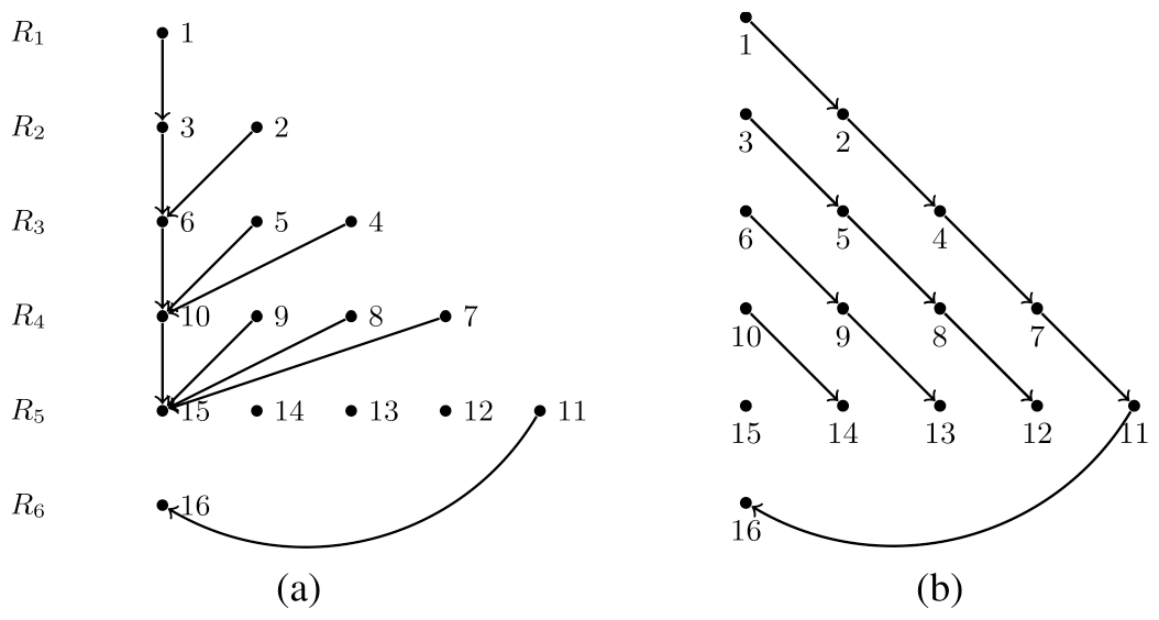
Figure A1 Visualization of black-box function dependencies in the reduction from HCP to WFYP-DEC, exemplified for the graph with n=5 nodes. Arcs in (a) represent the dependencies in the constructed farm (i.e., which turbines bear influence on which others) for the first two cases in Eq. (A2), while arcs in (b) represent those for the remaining cases in Eq. (A2). Note that actual function values depend on input x.

This completes the construction of a WFYP-DEC instance $(T,\mathcal{L},\mathit{\{}{\mathrm{\Gamma }}_i{\mathit{\}}}_{i\in T},f_{\mathit{\omega }}^{\mathrm{\Sigma }},F)$ from the input HCP instance G. Note that the reduction (dimensions, all arithmetic operations, and constructed numbers) clearly requires only polynomial time and space with respect to the size of the input; in particular, the objective function can be evaluated in 𝒪(n³), since $\left|T\right|=n_{\mathrm{WT}}={\mathrm{\Delta }}_n+\mathrm{1}\le n^{\mathrm{2}}$ and ${n_{\mathrm{\Gamma }}}_i=n$ for all i∈T. (In fact, it can easily be seen that our reduction allows the “strong” part of 𝒩𝒫 hardness to carry over from the HCP; cf. Garey and Johnson, 1979.)

It remains to be seen that the given graph contains a Hamiltonian circuit ℛ if and only if the constructed WFYP-DEC instance $(T,\mathcal{L},\mathit{\{}{\mathrm{\Gamma }}_i{\mathit{\}}}_{i\in T},f_{\mathit{\omega }}^{\mathrm{\Sigma }},F)$ allows a solution x with objective value $f_{\mathit{\omega }}^{\mathrm{\Sigma }}\left(x\right)\ge F=n$. To that end, we first assume that $\widehat{x}\in \mathit{\{}\mathrm{0},\mathrm{1}{\mathit{\}}}^{({\mathrm{\Delta }}_n+\mathrm{1})n}$ is a feasible solution for WFYP-DEC (so every turbine is assigned exactly one yaw offset) with objective value $f_{\mathit{\omega }}^{\mathrm{\Sigma }}\left(\widehat{x}\right)\ge F$. Since by construction only n turbine yaw settings can possibly incur a profit of 1 each (and all others at most zero), $f_{\mathit{\omega }}^{\mathrm{\Sigma }}\left(\widehat{x}\right)=F=n$ does in fact hold, which also implies that the last case in the function definition (A2) never occurs (since otherwise $f_{\mathit{\omega }}^{\mathrm{\Sigma }}\left(\widehat{x}\right)\le \mathrm{1}-n+n=\mathrm{1}<n$ would hold – a contradiction). In particular, tracing the functional dependencies with regard to which yaw offset assignments incur which costs for subsequent turbines (in the “cascading” row sets), we can conclude that no yaw offset is chosen twice among turbines $\mathrm{1},{\mathrm{\Delta }}_{\mathrm{2}},{\mathrm{\Delta }}_{\mathrm{3}},\mathrm{\dots },{\mathrm{\Delta }}_n$. Moreover, due to the first two cases in Eq. (A2) (and since $\widehat{x}$ represents a feasible yaw configuration) and because every turbine has the same set of n admissible yaw offsets, it holds that each yaw offset is chosen exactly once for this set $\mathit{\{}\mathrm{1},{\mathrm{\Delta }}_{\mathrm{2}},{\mathrm{\Delta }}_{\mathrm{3}},\mathrm{\dots },{\mathrm{\Delta }}_n\mathit{\}}$ of turbines. Furthermore, note that by definition, any yaw setting j for turbines $i={\mathrm{\Delta }}_{k-\mathrm{1}}+\mathrm{1}$, $k=\mathrm{2},\mathrm{\dots },n$ incurs a profit of either 1−n or 0 but that since $f_{\mathit{\omega }}^{\mathrm{\Sigma }}\left(\widehat{x}\right)=n$, the respective settings prescribed by $\widehat{x}$ in fact all yield zero profit. Thus, these costs necessarily arise from the third case in Eq. (A2), which means that turbines ${\mathrm{\Delta }}_{\mathrm{1}}+\mathrm{1},{\mathrm{\Delta }}_{\mathrm{2}}+\mathrm{1},\mathrm{\dots },{\mathrm{\Delta }}_{n-\mathrm{1}}+\mathrm{1}$ all have the same yaw offset as turbine 1. Consequently, by the fourth case in the definition, the yaw configurations chosen for turbines Δ₁=1 and Δ_n+1 are also identical.

We can now construct a Hamiltonian circuit in G from this WFYP solution $\widehat{x}$: starting at vertex $v_{p_{\mathrm{1}}}\in V$, where p₁∈[n] is the yaw offset chosen for turbine Δ₁=1, we visit the other n−1 nodes in the order prescribed by the yaw offsets selected for turbines ${\mathrm{\Delta }}_{\mathrm{1}},\mathrm{\dots },{\mathrm{\Delta }}_n$ and finally move from the last node back to $v_{p_{\mathrm{1}}}$. Indeed, this traversal produces the tour $\widehat{\mathcal{R}}=\mathit{\left\{}\mathit{\right\{}{v}_{p_{\mathrm{1}}},v_{p_{\mathrm{2}}}\mathit{\}},\mathit{\{}{v}_{p_{\mathrm{2}}},v_{p_{\mathrm{3}}}\mathit{\}},\mathrm{\dots },\mathit{\{}{v}_{p_{n-\mathrm{1}}},v_{p_n}\mathit{\}},\mathit{\{}{v}_{p_n},v_{p_{\mathrm{1}}}\mathit{\left\}}\mathit{\right\}}$, which shows that a “yes” answer for the constructed WFYP-DEC instance yields a “yes” answer for the original HCP instance.

For the converse direction, let a circuit $\widehat{\mathcal{R}}=\mathit{\left\{}\mathit{\right\{}{v}_{\mathit{\pi }\left(\mathrm{1}\right)},v_{\mathit{\pi }\left(\mathrm{2}\right)}\mathit{\}},\mathrm{\dots },\mathit{\{}{v}_{\mathit{\pi }(n-\mathrm{1})},v_{\mathit{\pi }\left(n\right)}\mathit{\}},\mathit{\{}{v}_{\mathit{\pi }\left(n\right)},v_{\mathit{\pi }\left(\mathrm{1}\right)}\mathit{\left\}}\mathit{\right\}}$ be a “yes” certificate for the given HCP instance G. Then, we can derive a solution $\widehat{x}$ with cost $f_{\mathit{\omega }}^{\mathrm{\Sigma }}\left(\widehat{x}\right)=n=F$ for the constructed WFYP-DEC instance from $\widehat{\mathcal{R}}$ as follows: for turbines 1, Δ₂, Δ₃, …, Δ_n, Δ_n+1, we respectively select the yaw offsets corresponding to the indices of the vertices in the order prescribed by the tour $\widehat{\mathcal{R}}$, starting (and ending) at $v_{p_{\mathrm{1}}}=v_{\mathit{\pi }\left(q\right)}$ for some q∈[n]; i.e., we set ${\widehat{x}}_{\mathrm{1},\mathit{\pi }(q+\mathrm{1})}={\widehat{x}}_{{\mathrm{\Delta }}_{\mathrm{2}},\mathit{\pi }(q+\mathrm{2})}=\mathrm{\dots }={\widehat{x}}_{{\mathrm{\Delta }}_n,\mathit{\pi }(q+n)}={\widehat{x}}_{{\mathrm{\Delta }}_n+\mathrm{1},\mathit{\pi }\left(q\right)}=\mathrm{1}$ (yielding total profit $\mathrm{0}+n\cdot \mathrm{1}=n$), while the entries corresponding to these turbines and the respective remaining yaw offsets are all set to zero. For the remaining turbines, we pick yaw offsets that incur no negative profits; i.e., for any $k=\mathrm{2},\mathrm{\dots },n$, turbine $i\in R_k\backslash \left(\mathrm{\Delta }\right(n)\cup \mathit{\{}{\mathrm{\Delta }}_n+\mathrm{1}\mathit{\left\}}\right)$ is assigned the same yaw offset as turbine $i-k+\mathrm{1}$, all with profit 0. Since this way every turbine is assigned exactly one yaw offset, $\widehat{x}$ indeed describes a feasible yaw configuration, and, by construction, its objective function value corresponds to $f_{\mathit{\omega }}^{\mathrm{\Sigma }}\left(\widehat{x}\right)=n=F$. This shows that the constructed WFYP-DEC instance also has a “yes” answer, which completes the proof. □

A5 Remark

We remark that the above construction could easily be adapted so that only non-negative terms can occur in the objective⁴, as would be the case in our application when focusing solely on power generation. Note also that, due to the generality of the black-box function $f_{\mathit{\omega }}^{\mathrm{\Sigma }}$ in WFYP-DEC, it is unclear whether one could always find a rational certificate of an arbitrary “yes” instance, so containment in the complexity class 𝒩𝒫 (and thus 𝒩𝒫 completeness) remains open. However, more importantly, we can slightly modify the proof of Theorem A4 to obtain the following inapproximability result.

A6 Corollary

There is no polynomial-time α-approximation algorithm for WFYP, for any α≤1, unless 𝒫=𝒩𝒫.

Proof. Revisiting the construction from the proof of Theorem A4, we modify the function values in Eq. (A2) to 0, δ, δ, δ, and −ε for the five cases, respectively, which then establishes the existence of a Hamiltonian circuit in G if and only if there is a feasible WFYP solution with value $\frac{\mathrm{1}}{\mathrm{2}}(n^{\mathrm{2}}+n-\mathrm{2})\mathit{\delta }$. Let $\mathit{\epsilon }:=\frac{\mathrm{1}}{\mathrm{2}}(n^{\mathrm{2}}+n-\mathrm{4})$ and $\mathit{\delta }:=\mathrm{4}({\mathrm{\Delta }}_n+\mathrm{1})\mathit{\epsilon }=n^{\mathrm{4}}-\mathrm{3}{n}^{\mathrm{2}}+\mathrm{6}n-\mathrm{8}$. Then, if the original HCP instance was a “yes” instance, any non-optimal solution of the constructed WFYP instance has a solution value of at most $\frac{\mathrm{1}}{\mathrm{2}}(n^{\mathrm{2}}+n-\mathrm{4})\mathit{\delta }-\mathit{\epsilon }$.⁵ Now suppose there exists a polynomial-time α-approximation algorithm for some arbitrary $\mathrm{1}/(n^{\mathrm{2}}+n-\mathrm{1})<\mathit{\alpha }\le \mathrm{1}$. Since any non-optimal solution (for a WFYP instance constructed from an HCP “yes” instance) has a value of at most $\frac{\mathrm{1}}{\mathrm{2}}(n^{\mathrm{2}}+n-\mathrm{4})\mathit{\delta }-\mathit{\epsilon }$ but the α-approximation algorithm outputs a solution with a value of at least $\mathit{\alpha }\cdot (n^{\mathrm{2}}+n-\mathrm{2})\mathit{\delta }/\mathrm{2}$, it can only be the case that the solution computed by the algorithm is non-optimal if

$$\begin{array}{lcll}& & \mathit{\alpha }& \left(\frac{n^{\mathrm{2}}+n-\mathrm{2}}{\mathrm{2}}\right)\mathit{\delta }\le \left(\frac{n^{\mathrm{2}}+n-\mathrm{4}}{\mathrm{2}}\right)\mathit{\delta }-\mathit{\epsilon }\\ \iff & & \mathit{\alpha }& \le \frac{n^{\mathrm{2}}+n-\mathrm{4}}{n^{\mathrm{2}}+n-\mathrm{2}}-\frac{\mathrm{2}\mathit{\epsilon }}{n^{\mathrm{2}}+n-\mathrm{2}}\\ & & & =\mathrm{1}-\frac{\mathrm{2}}{n^{\mathrm{2}}+n-\mathrm{2}}-\left(\mathrm{1}-\frac{\mathrm{2}}{n^{\mathrm{2}}+n-\mathrm{2}}\right)=\mathrm{0},\end{array}$$

which contradicts the prerequisite $\mathit{\alpha }>\mathrm{1}/(n^{\mathrm{2}}+n-\mathrm{2})>\mathrm{0}$. Thus, the α-approximation algorithm does, in fact, always yield an (optimal) solution of value $\mathit{\alpha }(n^{\mathrm{2}}+n-\mathrm{2})\mathit{\delta }/\mathrm{2}$ if and only if the input HCP instance was a “yes” instance. It could therefore be used to decide the existence of a Hamiltonian circuit in polynomial time, contradicting the 𝒩𝒫 hardness of the HCP. To see that this implies that no polynomial-time α approximation can exist (provided 𝒫≠𝒩𝒫) for any $\mathrm{0}<\mathit{\alpha }\le \mathrm{1}$, it suffices to observe that $\mathrm{1}/(n^{\mathrm{2}}+n-\mathrm{2})\to \mathrm{0}$ as n→∞. □