Wind resources of southeast Australia during peak electricity demand days

Peaks in electricity demand are critical times when it is important to understand the contribution of wind energy to the supply of electricity. In southeast Australia, peaks in electricity demand may be caused by unusually hot or cold periods that correspond to increased cooling and heating loads, respectively. These peaks in demand tend to be centred in the morning and early-evening hours as a result of consumption patterns and behind-the-meter solar generation during the middle of the day.

In this study, we examine the characteristics of the southeast Australian wind energy resource on days when the electricity demand is above the 80th percentile for heating and cooling days, respectively. We use a 29-year dataset of reanalysis over Australia. To correct for changes to the electricity system and consumption patterns in this period, a random forest model is fitted that relates the meteorological conditions to the electricity demand during a recent 4-year period.

We find positive wind generation capacity factors over many offshore parts of the region during both high-demand hot days and high-demand cold days. Over land, areas of complex topography show positive capacity factor anomalies on high-demand cold days, while other areas show negative capacity factor anomalies. Reverse patterns are found on high-demand hot days. It is shown that high-demand hot days are associated with a blocking high in the Tasman Sea, while high-demand cold days can be split into cold, wet, and windy outbreaks and high-pressure systems associated with light winds. On high-demand hot days, the peak in the diurnal cycle of wind in the offshore declared development area in southeast Australia is aligned with the peak in electricity demand, while high-demand cold days show little systematic diurnal variability.

1 Introduction

Spatial and temporal variability of wind power in the mid-latitudes is caused by both synoptic and local-scale atmospheric phenomena. On a synoptic-scale, the near surface wind variability follows the passage of cyclonic and anti-cyclonic pressure anomalies. In southeast Australia, which is a favourable area for offshore and onshore wind energy development, the near-surface wind field is strongly modulated by weather systems such as cold fronts, low-pressure systems or blocking highs to the east leading to strong northerly winds. For example, in southeast Australia, cold fronts can be defined as a shift in wind direction from the northwest to southwest quadrants (Simmonds et al., 2012), while heat waves are often associated with strong northerly winds (e.g. Pezza et al., 2012; Wei et al., 2023). Pichault et al. (2021) showed that around 46 % of ramp events at a SE Australia wind farm were due to frontal or post-frontal activity.

Local processes also influence variation in wind power on shorter timescales. These processes are important because electricity demand also has a significant diurnal cycle, with a consistent “duck-curve” shape (Simshauser and Wild, 2025; Restel and Say, 2025) arising from the combination of peak electricity usage in the morning and early evening, together with peak behind-the-meter solar production during the middle of the day. For example, Huang et al. (2023) used commercial aircraft measurements to examine the diurnal cycle of the boundary layer wind on heat-wave and non-heat-wave days in Melbourne, Australia. They found systematically higher wind speeds from the early hours of the morning until midday on heat-wave days relative to non-heat-wave days, which they attribute to momentum transfer to the surface associated with the nocturnal low-level jet. This emphasises that the variation in wind power is a combination of synoptic-scale processes and local-scale processes, some of which will exhibit a pronounced diurnal cycle. Numerous other studies have found a systematic diurnal variation in wind speed in coastal areas, including Xia et al. (2022), who found a maximum in wind speed during the afternoon and night at an offshore site on the east coast of the US, and Brown et al. (2017), who found a diurnal variation in wind speed and direction linked to the land–sea breeze circulation over coastal areas of the Northern Territory, Australia. The Australian Energy Council estimates that 40 % of Australia's residential energy usage is from air heating and cooling (AEC, 2022). While some of this heating comes from gas, passive solar or wood fires, the majority comes from electricity. This means that the same meteorological drivers that influence the near-surface wind speed and wind power availability can also influence the electricity demand. For example, Ashcroft et al. (2009) defined cold events in Melbourne in the lowest 0.4 % of maximum temperatures and showed that these events are associated with south to southwesterly geostrophic flow. These days had an average temperature of 7.8 °C in July and an average temperature of 16.8 °C in January, indicating that they all would have been high-heating-demand days. These events simultaneously influence both the electricity demand and the wind energy supply.

The coupling of both wind energy generation and electricity demand to the weather raises the possibility of systematic patterns of supply on the highest (or peak) demand days. High-demand summer days are strongly influenced by air-conditioning loads (AEMO, 2024), while high-demand winter days are strongly influenced by heating loads (AEMO, 2025). For example, Liu and Bai (2023) found that on heat-wave days in China, there was a greater diurnal cycle of wind power in many parts of China, with systematic below-average wind power during the morning hours and above-average wind power during the night. Similarly, they found above-average wind power during cold-wave conditions in all regions of China. The temperature is not the only meteorological parameter that may influence human decisions around air-conditioning and heating. For example, the ERA5 HEAT dataset uses air temperature, humidity and radiation to derive a thermal comfort index (Napoli et al., 2021). These studies demonstrate the complex interplay between energy consumption and diverse meteorological parameters.

Recently, several studies have addressed the variability of the wind energy generation in Australia, with particular reference to the multi-scale nature of the variability. Richardson et al. (2023) examined periods of solar and wind drought relative to the climate modes of the El Niño–Southern Oscillation (ENSO), the Indian Ocean Dipole (IOD) and the Southern Annular Mode (SAM). They also found that periods of solar drought coincide with positive or negative anomalies of temperature at 2 m above the ground, although they noted that cloudy solar-drought periods tended to be associated with cooler summertime temperatures and warmer wintertime temperatures, thus partly ameliorating the deficit in generation. Gunn et al. (2023) proposed an optimal layout of wind farms that could maximise the supply of wind energy but noted persistent variations due to ENSO. Vincent and Dowdy (2024) examined the wind energy resource over SE Australia according to its diurnal, seasonal and interannual variability. Notably, they found variations in the wind resource with ENSO, as well as distinct regional variation in the timing and amplitude of the diurnal cycle of wind speed.

The purpose of this study is to examine the wind resource across SE Australia on the highest-electricity-demand days in the region. Moreover, the synoptic patterns and diurnal variability on these days are examined in an attempt to understand the meteorological processes driving both wind generation and electricity demand. We use a moderately high resolution reanalysis over Australia with a horizontal grid spacing of 12 km, which will partially resolve local-scale variations in wind speed associated with topographic and coastal processes. We consider the ambient meteorology as the only predictor of high demand, rather than non-meteorological factors such as large public events or holiday periods. We account for technical changes to the electricity system by fitting a model that relates the demand profile of the 2015–2018 period to the meteorological conditions of the past 29 years (i.e. 1990–2018). In this way, we construct a consistent 29-year dataset of high-demand hot and cold days for which the average wind energy capacity factor (using a single representative wind turbine) and its synoptic patterns are examined. These high-demand hot and cold days are then categorised into high-wind-energy or low-wind-energy days in an Australian Government offshore declared area (which is likely to be the site of Australia's first offshore wind farms) for further analysis.

In this paper, we describe the datasets used and the estimation method to determine high-demand hot and cold days in Sect. 2. In Sect. 3 we present the average wind capacity factors and synoptic conditions on high-demand hot and cold days, followed by the synoptic patterns associated with high or low wind resources on these days. We then present the diurnal cycle of wind capacity factors specific to the offshore declared area and electricity demand on hot and cold high-demand days. Concluding remarks are given in Sect. 4.

2 Methods and data

2.1 Overview of methods

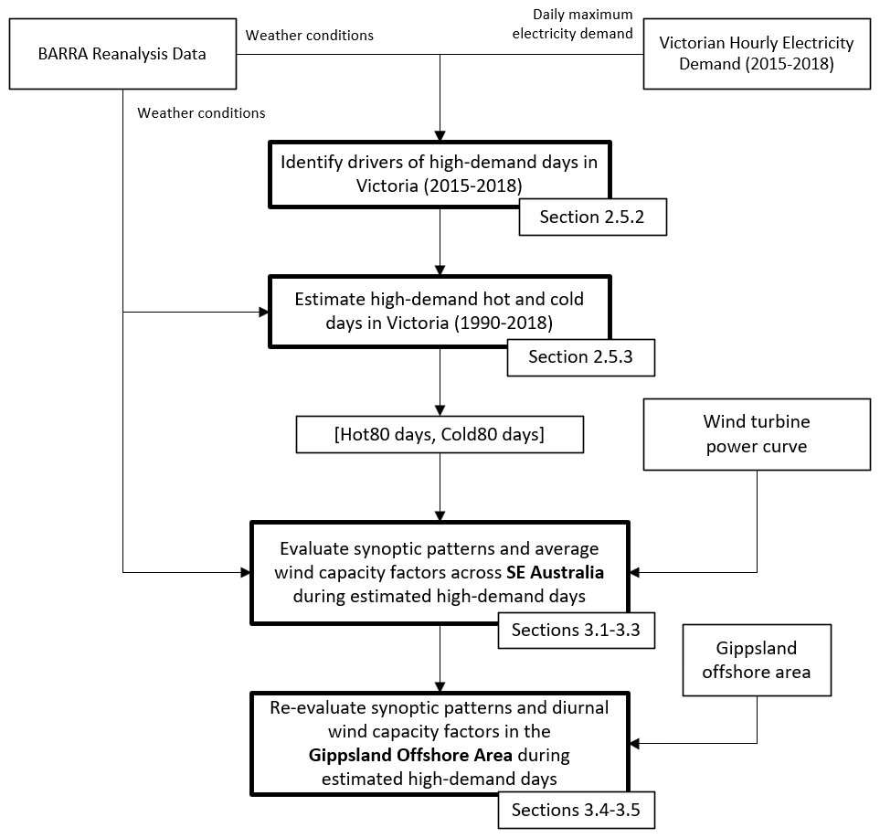
The structure of the data analysis is summarised in Fig. 1.

Figure 1 Research structure overview.

2.2 Reanalysis data

The wind speed data used in this study are from the Bureau's Atmospheric high-resolution Regional Reanalysis for Australia (BARRA) (Su et al., 2021), produced by the Australian Bureau of Meteorology. The data cover the time period 1990–2018 and are on a 12 km grid. The instantaneous wind components at the end of each time step from the reanalysis data were vertically interpolated to a height of 100 m above ground level using log-linear interpolation in height, using the model levels closest to 100 m, which had an average height of 76 and 109 m above ground level over the region of interest. This same dataset was used in Vincent and Dowdy (2024) to characterise the diurnal and interannual variability in wind speed over SE Australia. The same ACCESS model that drives the BARRA reanalysis, but with a horizontal grid spacing of 4 km, was used to examine the land–sea breeze circulation in northern Australia in Brown et al. (2017). They compared the land–sea breeze anomalies with those from scatterometer observations and found reasonable agreement, albeit with some errors in the direction of the perturbations around areas of complex coastline. Errors in the fine-scale structure of the sea breeze are likely present in the data that we use here too, although we note that the Gippsland offshore wind energy declared area is adjacent to a relatively straight coastline with the complex topography set back from the coast.

2.3 Electricity demand data

Hourly electricity demand data for the state of Victoria were sourced from OpenElectricity (2025). We note that rooftop solar generation is an implicit part of the electricity demand data as it is recorded as negative demand after being first consumed behind the meter. This results in an observable reduction in daytime electricity demand at the system level. This means that the high-demand days studied here are days where there was still a high demand after rooftop solar energy had been consumed, and therefore these are days when it would be critical for an energy source other than rooftop solar to make a large contribution to electricity generation. These days are arguably the days when wind energy has the biggest role to play in achieving net-zero emissions, because this demand is currently being met mostly by non-renewable energy generation.

2.4 Capacity factor estimations

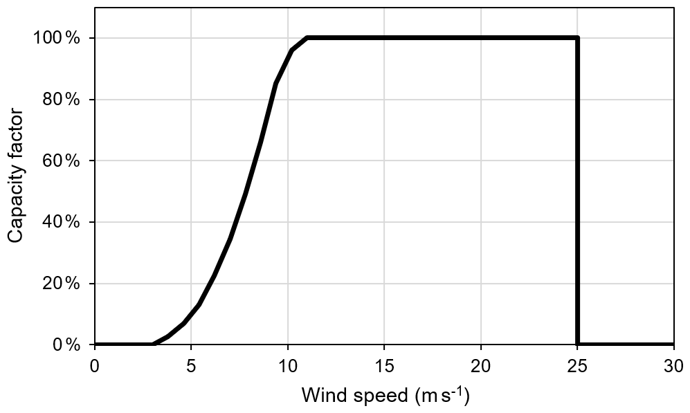
Wind turbine capacity factors were estimated from wind speed data at 100 m from the BARRA reanalysis using a typical power curve with a cut-in wind speed of 3.8 m s⁻¹, a rated capacity of 11 m s⁻¹ and a cut-out wind speed of 25 m s⁻¹ (Fig. 2) as a representative wind turbine. This is similar to the specifications of other offshore turbines, for example, Siemens Gamesa SG 14-222 DD and MHI Vestas Offshore V164-8.8 MW (Wind Turbine Models, 2025; Ohlendorf and Schill, 2020). The wind speed that is used to calculate the capacity factor is an instantaneous wind speed but pertains to a grid point of spatial area 12 × 12 km. It was shown in Brown et al. (2024) that convective gusts are severely underrepresented in a similar version of BARRA to that used here, and we acknowledge that future studies must focus on convection-permitting models and the sub-hourly timescales to properly resolve wind farm cut-out scenarios. Wake effects were not included in this calculation, due to the coarse-resolution data used and single turbine assumption, and for the purpose of this study, density effects were not included.

Figure 2 Wind turbine power curve.

2.5 Estimating high-demand hot days and high-demand cold days

As shown in Fig. 1, high-demand hot days and high-demand cold days are estimated based on actual electricity consumption during the years 2015–2018 in the Victorian electricity grid (which has its largest electricity demand in the Melbourne metropolitan area). This choice of years is motivated by this being a recent period but prior to the COVID19 pandemic (when consumption patterns changed in unexpected ways). The following steps are used to identify likely days from the period 1990–2018 that would likely have been high-demand days, given consumption patterns similar to those in the 2015–2018 period.

2.5.1 Classification of days as high-demand hot days or high-demand cold days

All days in the 2015–2018 period were classified as cooling degree days or heating degree days, following the definitions of the Australian Energy Market Operator (AEMO, 2023) for Victoria. The cooling degree index (CDI) and heating degree index (HDI) are calculated according to Eqs. (1) and (2), using average meteorological values from BARRA from a subset of the Melbourne metropolitan area (Fig. 5). Using this approach, days with an average temperature greater than 18 °C will have a positive CDI value, indicating increasing air-conditioning usage, and days with an average temperature less than 16.5 °C will have a positive HDI value, indicating increasing heating demand.

$$\begin{array}{}\text{(1)}& {\displaystyle }\text{CDI}=\max (\mathrm{0},\stackrel{\mathrm{‾}}{T}-\mathrm{18}),\text{(2)}& {\displaystyle }\text{HDI}=\max (\mathrm{16.5}-\stackrel{\mathrm{‾}}{T},\mathrm{0}),\end{array}$$

where $\stackrel{\mathrm{‾}}{T}$ is the daily average temperature from 09:00 p.m. local solar time (LST) the night before to 09:00 p.m. LST on the current day.

The set of days in the period 2015–2018 was subset into days with a positive CDI or positive HDI. Respectively, these are the days that are likely to be dominated by either air-conditioning or heating loads, and as such these two sets of days are treated separately in this study. For the purpose of this study, we consider days where the electricity demand was in the top 20 % of all electricity demand days as high-demand days. We therefore construct two sets of days: high-demand hot days indicating significant air-conditioning usage (hereafter Hot80 days) and high-demand cold days indicating significant heating usage (hereafter Cold80 days) (Vincent et al., 2025).

2.5.2 Linear regression and random forest models of high-demand days: model selection

We tested two classes of models for predicting whether a given day would be a high-demand day or would not be a high-demand day: a multiple linear regression (LR) model and a random forest (RF) model. In both cases, the inputs to the models were meteorological variables from the BARRA reanalysis averaged over the Melbourne basin area: heating degree index (HDI), cooling degree index (CDI), maximum temperature (Tmax), average temperature (Tav), wind speed (WS), wind chill factor (WC) calculated following Osczevski and Bluestein (2005), daily average relative humidity (RH), incoming shortwave radiation (SWD), and a binary variable indicating whether it was a weekday or weekend day (DOW). We also include the temperature on the previous day (Tmax_lag1) as a predictor. For each of the high-demand hot days and high-demand cold days, half the days were randomly chosen as a training dataset, and the other half were assigned to a testing dataset using a fixed random seed for reproducibility. For the multiple linear regression model, the output was a continuous variable, which was converted to a binary variable based on the criteria of whether it exceeded the 80th percentile of demand or not, while the random forest model directly predicted a binary outcome. In both cases, models were evaluated using the false-alarm rate (FAR) and probability of detection (POD) (Wilks, 2011).

For the linear regression model, every possible combination of predictors was tested, and the best performing models were selected. The predictors for the best performing model for high-demand hot days were CDI ($p=\mathrm{1.3}\times {\mathrm{10}}^{-\mathrm{6}}$), Tmax (p=0.48), Tav (p=0.041), RH (p=0.12), WS (p=0.093) and DOW ($p=\mathrm{4.6}\times {\mathrm{10}}^{-\mathrm{8}}$), where all predictors were significant at the 5 % level except for RH and Tmax, while the predictors for the best performing model for high-demand cold days were HDI ($p=\mathrm{3.3}\times {\mathrm{10}}^{-\mathrm{6}}$), Tmax (p=0.0022), RH (p=0.0042), Tmax_lag1 ($p=\mathrm{1.96}\times {\mathrm{10}}^{-\mathrm{9}}$) and DOW (p=0), where all predictors were significant at the 5 % level, noting that there are more HDI days (952) than CDI days (384), which contributes to the lower p values.

The random forest model was run 100 times using all predictors. For each model realisation, the predictors were arranged in order of importance, and only the variables comprising the cumulative top 80 % in importance were retained. Although there was some variation in the order of the most important predictors, the same set of most important predictors were selected in all 100 realisations in the case of the Hot80 models and in 68 % of the 100 realisations in the case of the Cold80 models. For the Hot80 days, the predictors selected and their average importance were Tav (29 %), CDI (26 %), Tmax (22 %) and RH (10 %), while for the Cold80 days, the predictors selected and their average importance were WC (20 %), Tav (19 %), Tmax (17 %), HDI (14 %), Tmax_lag1 (12 %) and DOW (11 %). The model was then re-trained using only these predictors.

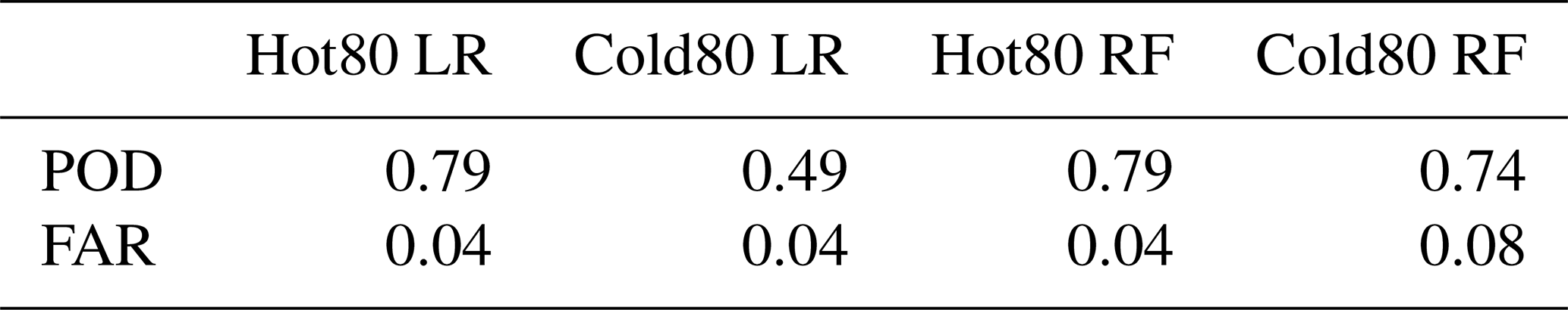
The POD and FAR of the selected multiple linear regression models and random forest models for the Hot80 and Cold80 days are shown in Table 1, indicating a better performance of the RF models relative to the LR models. This is particularly evident for the Cold80 models, where the distinct synoptic patterns leading to cold high-demand days, as discussed further in Sect. 3.4, mean that a linear model does not perform well.

Table 1 POD and FAR scores for the fitted LR and RF models for the Cold80 and Hot80 days.

2.5.3 Model prediction for the 29-year period

The chosen RF model was applied to the full dataset from 1990–2018 to identify Hot80 and Cold80 days. To ensure consistency of the RF model, the random forest was refitted 1000 times, with the same set of predictors but different random seeds. Only days that were identified as high-demand days in at least half of these 1000 runs were included in the set of high-demand days for the subsequent days. There were 51 (288) days that appeared in more than zero but less than 500 of the 1000 realisations for the Hot80 (Cold80) days. This left a total of 439 Hot80 days and 1363 Cold80 days in the 29-year period for further analysis.

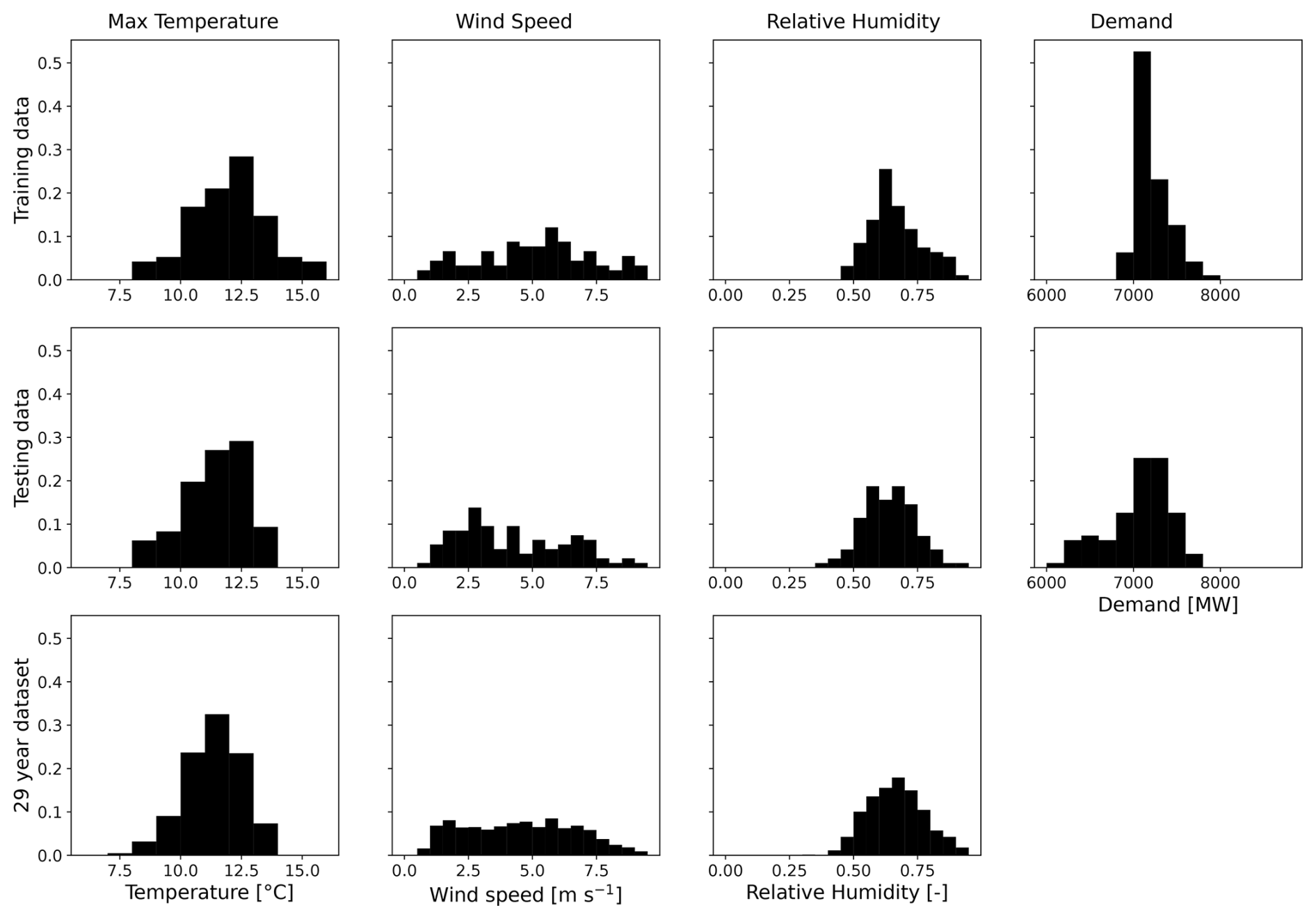
The distributions of maximum daily temperature, wind speed and relative humidity of the Hot80 and Cold80 days for the training dataset (based on actual demand), the testing dataset (based on predicted demand from the RF model) and the 1990–2018 period (based on predicted demand from the RF model) are shown in Figs. 3 and 4. The histograms indicate similar sets of meteorological conditions on both the actual and predicted sets of high-demand days for both hot and cold days. The Hot80 days tend to have low relative humidity and moderate wind speed, while the Cold80 days tend to have high relative humidity and little dependence on wind speed.

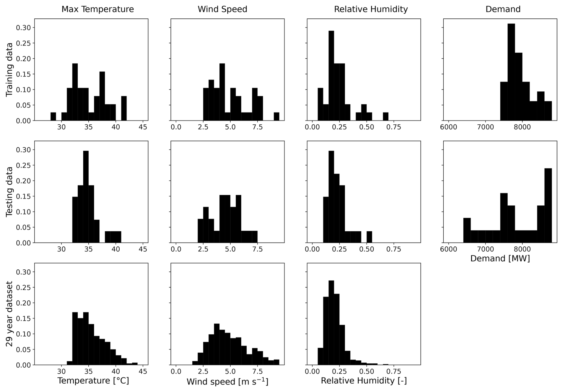
Figure 3 Histograms of maximum daily temperature, wind speed, relative humidity and demand for the training data (top row), testing data (middle row) and the full 29-year dataset for Hot80 days. The data in the top row are based on actual high-demand days, while the data in the second and third rows are based on the modelled high-demand days from the RF model.

Figure 4 As for Fig. 3 but for Cold80 days.

2.6 The Gippsland offshore area

Recently, the Australian Government announced priority areas for the development of offshore wind (Department of Climate Change, Energy, the Environment and Water, The Australian Government, 2024). One of these areas is located in the Gippsland region of southeast Australia, and significant progress has already been made in preparation for offshore wind energy in this region. We therefore chose to focus on the role that this region could play in meeting Victoria's energy needs on high-demand days. For the purpose of this study, the wind resource has been analysed in a simplified polygon corresponding to the intersection of the Gippsland priority area with the grid points of the BARRA reanalysis (Fig. 5).

3 Results

3.1 Average wind capacity factors over southeast Australia

The average wind capacity factors over southeast Australia are shown in Fig. 5, based on the BARRA reanalysis data interpolated to 100 m. The average capacity factors are calculated by applying the wind turbine power curve (Fig. 2) to all wind speed data and then averaging over the 29-year dataset. As expected, higher capacity factors are found over the ocean and over flat terrain inland. Lower capacity factors are found over areas of elevated topography to the southeast of the land region. As discussed in Vincent and Dowdy (2024), this is broadly consistent with higher-resolution analyses but lacks the enhanced wind speeds at the highest peaks of the topography, e.g. Davis et al. (2023).

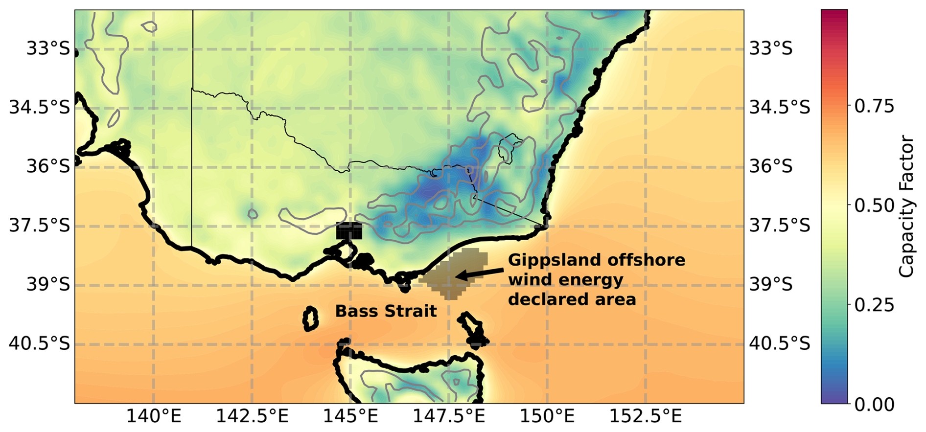
Figure 5 Average wind capacity factors across SE Australia. Coastlines and state boundaries are shown in thick and thin black lines, respectively. Topography contours are shown as thick grey lines at levels 400, 800, 1200 and 1600 m. Grid points in the BARRA dataset corresponding to the Gippsland offshore wind energy declared area are shaded in grey, and the grid points corresponding to metropolitan Melbourne that are used for prediction of high-demand days are shaded in black.

3.2 Capacity factor anomalies on Victorian high-demand hot and cold days

In Fig. 6, the average capacity factor anomalies are shown for Hot80 and Cold80 days. Statistically significant positive anomalies are found over most areas of the coastal ocean regions for both Hot80 and Cold80 days, indicating favourable conditions for offshore wind on these days. Over regions of elevated topography, negative capacity factor anomalies are found on Hot80 days, while positive capacity factor anomalies are found on Cold80 days. Inland, over flatter terrain, the opposite is found, although the anomalies are generally small in magnitude on the Cold80 days.

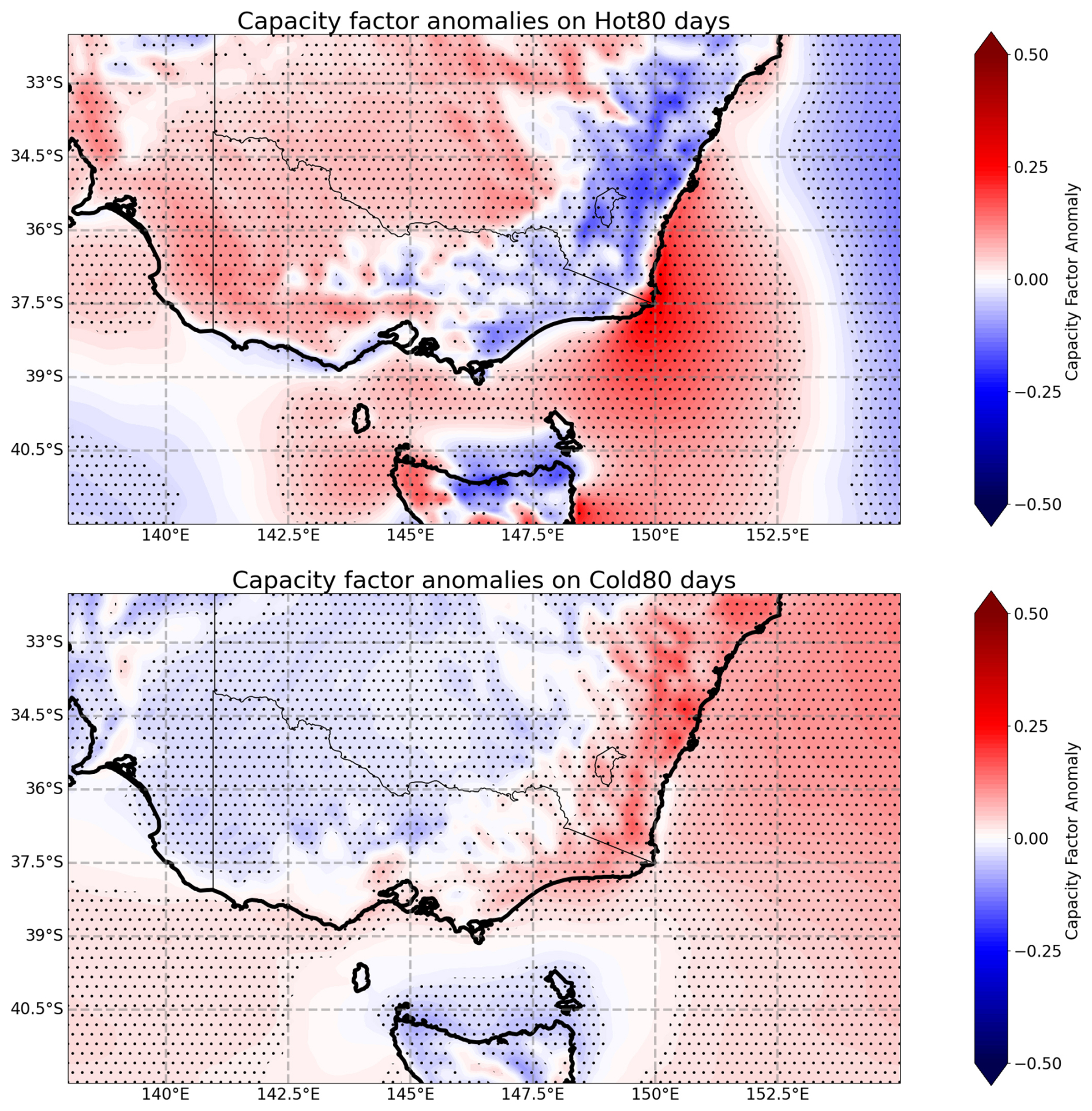
Figure 6 Composite capacity factor anomalies on Hot80 and Cold80 days. Areas of statistical significance tested using a two-sided bootstrapping test at the 5 % significance level are shown with stippling.

3.3 Synoptic patterns on high-demand heating and cooling days

In this section, we examine the synoptic patterns associated with the capacity factor anomalies on Hot80 and Cold80 days (Fig. 7). This result suggests that, on average, Hot80 days are associated with a blocking high in the Tasman Sea, with northerly flow impacting much of eastern Australia. In contrast, the Cold80 days, on average, have a high-pressure system located over central Australia, with southwesterly flow impacting much of southeastern Australia. These results are typical of summertime and wintertime synoptic patterns in southeast Australia, but we note that no constraints were placed on the time of year when the Hot80 and Cold80 days occurred.

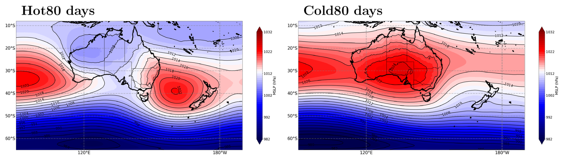
Figure 7 Composite mean sea level pressure at 00:00 UTC for Hot80 and Cold80 days.

3.4 Synoptic patterns associated with high-wind and low-wind conditions in the Gippsland offshore wind energy development region on high-demand days

We now examine whether there are Hot80 or Cold80 days for which offshore wind energy in the Gippsland region could play a particularly favourable or unfavourable role in contributing to the electricity system. This is achieved by dividing the Hot80 days into a subset of days with high average wind speed in the Gippsland offshore region (Fig. 5) (i.e. average capacity factor >0.9) and a subset of days with low average wind speed in the Gippsland offshore declared area (i.e. average capacity factor <0.3). The same process was followed for the Cold80 days, yielding four sets of days: Cold80 high-wind days, Cold80 low-wind days, Hot80 high-wind days and Hot80 low-wind days (Vincent et al., 2025). The average synoptic patterns for these four classes are shown in Figs. 8 and 9.

For the Hot80 days, Fig. 8 indicates that both the high- and low-wind cases have a similar synoptic pattern. In both cases, there is a high-pressure system in the Tasman Sea and northerly flow over southeastern Australia. This synoptic pattern is suggestive of both adiabatic warming associated with the high-pressure system and warm air advection associated with the northerly flow. The primary difference between the high-wind and low-wind cases is the strength of the trough approaching from the west, which in the high-wind case leads to a tightening of the isobars around the Gippsland region, while the low-wind case has a more zonal flow to the west and lighter winds throughout the Gippsland region.

For the Cold80 days, Fig. 9 indicates a completely different synoptic pattern for the high- and low-wind cases. The high-wind case (Fig. 9a) shows a cold front over southeast Australia, with strong southwesterly flow over all of southeast Australia. This indicates a likelihood of a favourable wind resource over a large portion of southeast Australia and not just over the Gippsland area. This synoptic type is likely to be associated with cold, wet and windy conditions. While not the focus of this study, it is noted that these conditions are probably associated with cloudy skies and a poor solar resource, indicating a positive role of onshore and offshore wind energy in the region.

The Cold80 low-wind case (Fig. 9b) indicates a high-pressure system over southeast Australia, suggestive of light winds throughout southeast Australia. Given that these days have already been identified as cold days, they are likely to be wintertime high-pressure systems when the subtropical ridge moves over the Australian continent and may be associated clear skies, strong radiative cooling, low temperatures and light wind at nighttime and in the early morning, as well as possibly sunny conditions later in the day. While these days are not suggestive of a good wind resource in the region, they may have a favourable contribution from solar energy in the wintertime sunny afternoons. The results in Fig. 9 suggest that there are at least two main profiles of cold days that impact the wind resource in Gippsland. These days will have a completely different profile of both demand and supply.

Figure 8 Composite mean sea level pressure for Hot80 (a) high-wind days and (b) low-wind days in the Gippsland offshore wind energy declared area (indicated by the yellow star).

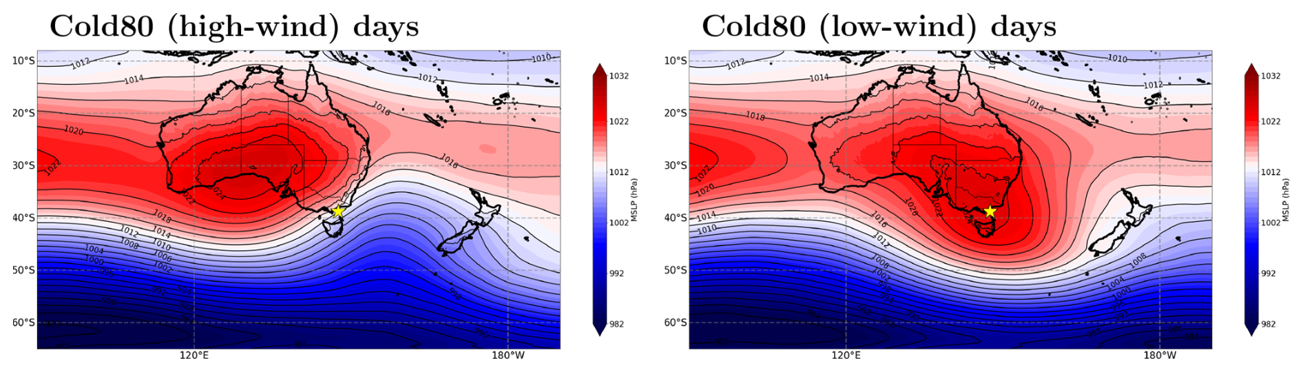
Figure 9 As for Fig. 8 but for Cold80 days.

3.5 The diurnal cycle of supply and demand on high-demand days in the Gippsland offshore region

Figures 8 and 9 indicate the possibility not only of different synoptic-scale processes but different mesoscale and diurnal processes influencing the wind resource. While these processes are not examined in detail here, we investigate the diurnal cycle of both capacity factor and electricity demand over the Gippsland offshore region for the four sets of days identified in Sect. 3.3.

Figure 10 shows the average diurnal cycle of capacity factor at the Gippsland offshore declared area on the high-wind, low-wind, Hot80 and Cold80 days. The most obvious result is that there is almost no diurnal cycle on the Cold80 days and a pronounced diurnal cycle on the Hot80 days with a peak at around 08:00 p.m. local time. It is also seen that the Hot80 diurnal cycle is curtailed on the high-wind days, which is likely partly due to the shape of the power curve and partly due to the fact that mesoscale processes such as sea breezes and low-level jets are sensitive to the background wind speed. We also note that the start and end points of these diurnal cycles do not precisely match up. This is because each composite diurnal cycle is constructed from a unique set of days that may climatologically be preceded or followed by a calmer or more windy day. We note that these diurnal cycles are based on the BARRA reanalysis with a horizontal grid spacing of 12 km. While this dataset has been shown to have a physically plausible representation of the diurnal cycle (Vincent and Dowdy, 2024), it will not capture all the mesoscale diurnal wind variations, particularly those associated with fine-scale variations in complex topography.

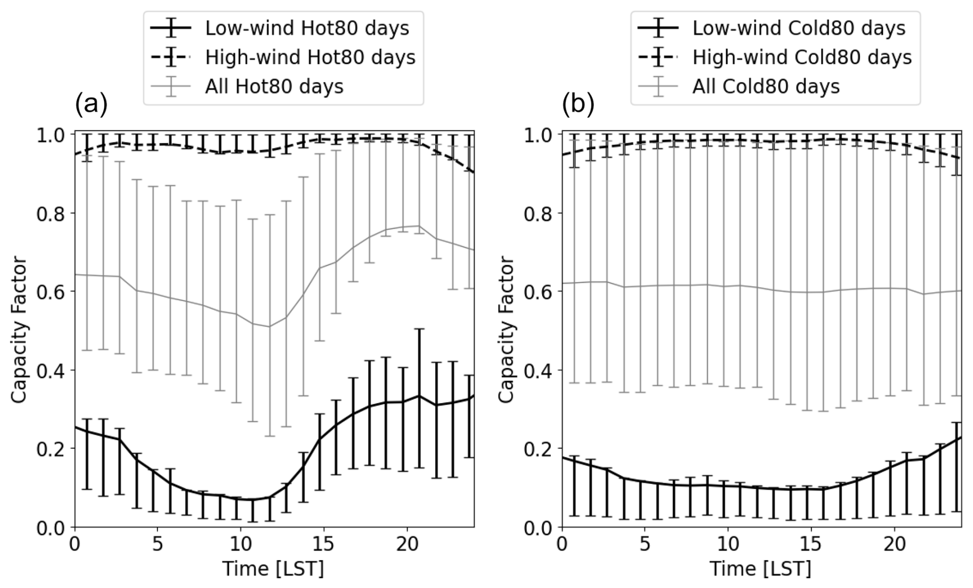
Figure 10 Average diurnal cycle of capacity factor over the Gippsland offshore area for (a) Hot80 days and (b) Cold80 days for all, high-wind and low-wind days. Error bars show the 33rd and 67th percentile capacity factor for each hour.

The diurnal cycle of electricity demand (Fig. 11) indicates a double demand peak on both Hot80 and Cold80 days, with a morning peak at around 07:00–08:00 a.m. LST and an early-evening peak at around 05:00–07:00 p.m. LST Note that these demand data are partly offset by rooftop solar before these data are collected and that hot days are generally likely to also be sunnier and have a larger solar resource than cold days (albeit with some penalty for heat-related impacts on solar panel performance that are considered a secondary effect here). There is a bigger dip in the middle of the day on the Cold80 days, likely because cold mornings tend to warm up during the middle of the day, while hot days get progressively hotter during the day. We also note that the early-evening demand peak is larger relative to the morning peak on Hot80 days than Cold80 days and that the early-evening peak on Hot80 days is partially aligned with the peak in capacity factor on these days. There is only a minor difference between the demand profile on high-wind and low-wind Hot80 and Cold80 days, and the differences are not statistically significant. We do note, however, less spread during the middle of the day on Hot80 low-wind days relative to Hot80 high-wind days, indicating more predictability at these times. Understanding the meteorological parameters associated with the spread in these demand profiles is a critical step for linking renewable electricity generation and demand on these days.

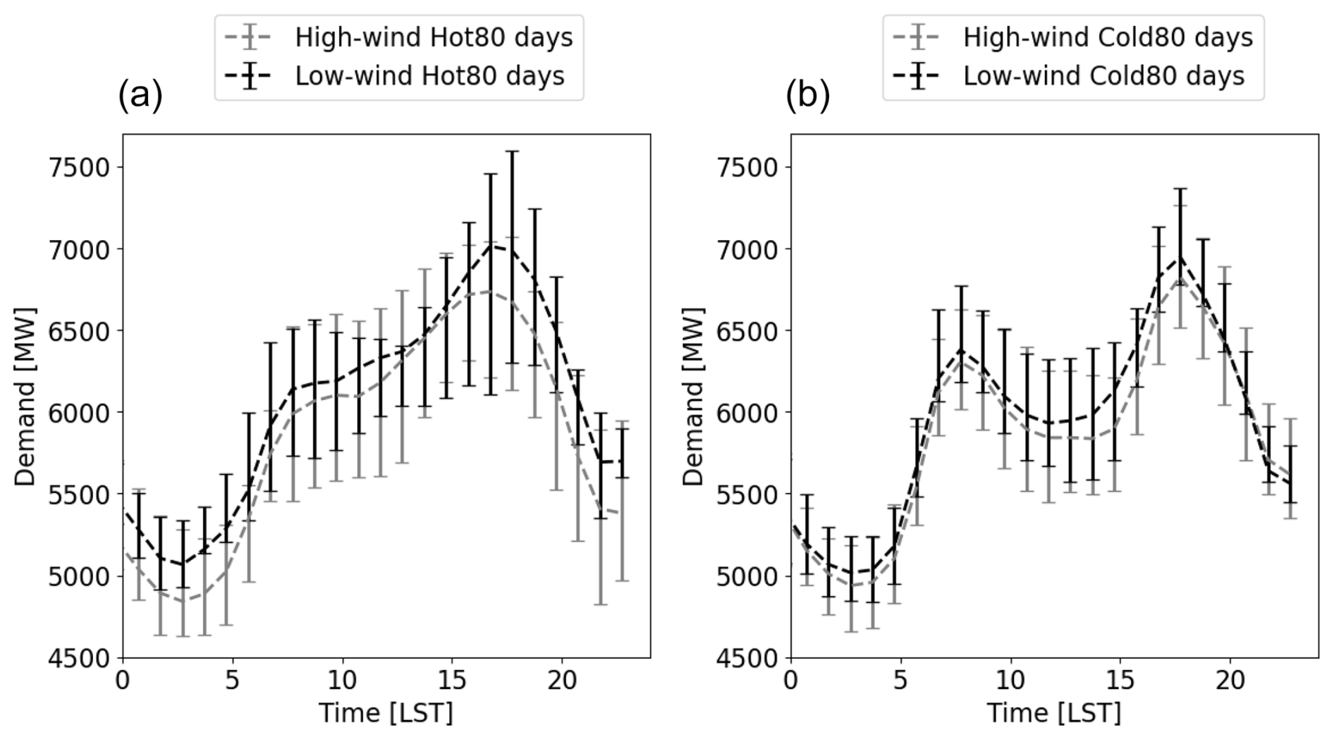
Figure 11 Average diurnal demand across Victoria for (a) Hot80 days and (b) Cold80 days for low-wind and high-wind days. Error bars show the 33rd and 67th percentile of demand for each hour.

4 Discussion and conclusions

The average wind resource in SE Australia is significantly different on high-demand hot days and high-demand cold days. The results presented here suggest decreased capacity factors over eastern Victoria and SE NSW on high-demand hot days, as well as increased capacity factors over western Victoria. An almost opposite pattern is found on high-demand cold days. This suggests the possibility of strategic placement of wind farms to target these highest-electricity-demand days in summer and winter.

The average synoptic pattern on high-demand hot days consists of a high-pressure system in the Tasman Sea, directing warm northerly flow over SE Australia. This pattern can lead to favourable wind conditions over SE Australia and the Gippsland offshore area. As well as the tightening of the isobars due to the approaching cold front on the high-wind, high-demand hot days, there is potential for some localised scale interactions that could influence the coastal wind resource in this region. For example, we note the more northerly location of the high-pressure system in the Tasman Sea under the low-wind cases, which directs northwesterly flow over the Bass Strait region, while the southerly displacement of the high-pressure system in the high-wind cases directs northerly flow over the Bass Strait region. Understanding the role of topography and possible channelling of the flow through the Bass Strait under different synoptic conditions might be important for understanding the wind variability in this region in the current and future climate. For example, a minor change in the climatological position of the Tasman Sea high could result in different local flows through the Bass Strait region. Moreover, localised wind phenomena such as sea breezes and low-level jets are likely to manifest as a scale interaction between the large-scale synoptic conditions and the locally experienced winds.

The average synoptic pattern on high-demand cold days can be split into two groups, depending on the strength of the wind in the Gippsland region. These two patterns relate to a cold air outbreak (Cold80 high-wind cases) and a high-pressure system over Victoria (Cold80 low-wind cases), respectively. The two scenarios lead to completely different wind patterns, with the former providing an excellent wind resource and the latter being associated with light winds.

The timing of the diurnal cycle of the wind capacity factor in the offshore Gippsland area is partly aligned with the diurnal cycle of electricity demand in high-demand hot days. This suggests that even if there is low-wind on high-demand hot days, the supply of wind energy in this offshore area still increases in line with the significant rise in early-evening electricity demand. As shown in Vincent and Dowdy (2024), the peak timing of the diurnal cycle of wind in SE Australia varies between offshore, coastal, mountainous and inland regions, which raises the importance of strategic placement of wind farms to help balance the daily cycle of electricity demand. Our results further suggest that on high-demand cold days there is very little systematic diurnal cycle of the wind capacity factor in the offshore Gippsland area. This means that the wind capacity factor in this area remains relatively stable across high-demand cold days and does not align with the diurnal variations of the electricity demand.

The results presented in this work show that there are meteorological drivers of both supply and demand on high-demand days and that these two factors must be examined together. While the variation manifests mostly in the wind resource, its co-variability with the variation in demand also needs to be understood. The most concerning days for the future electricity system are the days with high electricity demand and low electricity supply – for example, high-demand hot days with low wind speeds, noting that the synoptic pattern for this case is also suggestive of light winds in many other parts of the country. We also note that while certain scenarios may be associated with a favourable wind resource, this resource may be undermined by the co-occurrence of hazards – for example, the high-demand hot days are similar to the synoptic setup for heat-wave conditions (e.g. Henderson et al., 2024)) or when combined with an approaching cold front, fire weather risk (e.g. Reeder et al., 2015) in SE Australia. Similarly the high-demand cold days are likely to overlap with hazards associated with cold, wet and windy conditions (e.g. Ashcroft et al., 2009). Building a robust future renewable electricity system requires a granular examination of multiple scenarios that influence supply and demand as well as other energy-related risk factors. This includes those scenarios brought about by localised meteorological phenomena, particularly around complex terrain, which requires higher-resolution modelling than that used in this study. Furthermore, the single turbine assumption that underpins the capacity factor calculation could be improved by further incorporating common wind farm configurations and design typologies.