FastLE: a new load extrapolation method for site-specific wind turbines using the load distribution meta-model

To ensure the safety of wind turbines at specific sites, IEC 61400-1 mandates the extrapolation of loads as a key requirement. Given the variability in wind parameters across different turbine sites, particularly in complex terrains, this task demands significant computational resources for simulations. However, the method recommended in the standard falls short of providing comprehensive assessments and rapid iterations necessary for all turbine locations in wind farm optimization designs. This paper presents a rapid load extrapolation method, named FastLE, which is based on a load distribution meta-model and tailored for specific sites. Based on 20 test cases, the blade root out-of-plane bending moment for a 50-year return period was calculated using both the International Electrotechnical Commission method and the FastLE method introduced in this paper. Through comparative analysis, the mean absolute percentage error is only 3.165 %, and the computation time for a single calculation has been reduced from 20 h to less than 1 s. The results show that the FastLE method can complete load extrapolation calculations for wind turbines in seconds with high accuracy. This makes it suitable for ensuring structural integrity during iterations of wind farm layout optimization or turbine type optimization, thereby reducing the safety risks associated with wind turbines.

1 Introduction

With the rapid development of wind energy, a growing number of new wind farms are being designed and constructed worldwide (International Energy Agency, 2024). However, the frequency of safety incidents caused by load-related issues is also rising (International Electrotechnical Commission, 2019; Veers et al., 2019). As a result, the crucial role of load extrapolation in ensuring the structural integrity of wind turbines has garnered significant attention (Cao et al., 2018). For wind turbines, the loading conditions are contingent upon the turbulent inflow of wind across a spectrum of atmospheric conditions. Consequently, statistical extrapolation is essential for projecting long-term load profiles from limited simulation datasets. This predictive exercise is crucial for determining the load rates associated with key design scenarios outlined by the International Electrotechnical Commission (IEC) standards for wind turbine design (International Electrotechnical Commission, 2019). Similarly, it is common for different sites in the same wind farm to experience varying wind conditions. Therefore, it is essential to calculate the extrapolated loads for each individual site and compare them with the design loads to ensure the safety of the wind turbines (International Electrotechnical Commission, 2019). The IEC-recommended approach requires a minimum of 60 seeds to simulate 600 s load time series under normal operating conditions with high wind speeds. Moreover, it demands significant computational resources and considerable time for performing a 50-year extrapolation based on the distribution of load extremes (Fogle et al., 2008). This intensive requirement complicates the consideration of extrapolated loads during the iterative optimization of wind farm layouts and turbine types, leading to suboptimal solutions (Zhang et al., 2024; He et al., 2024) or protracted optimization periods (Sarcos et al., 2024). To address this challenge, there is a pressing need for a fast method to calculate extrapolated loads tailored to specific site wind conditions. This method would be essential for assessing safety risks associated with loads at various sites in a wind farm during the design phase. Furthermore, it would enable iterative optimizations in which extreme extrapolated loads serve as crucial constraints for enhancements in wind farm layout and turbine types.

Numerous studies have investigated methods for calculating extreme extrapolated loads. The latest version of the IEC 61400-1 standard mandates the calculation of these loads as a design requirement and presents two computational pathways: “fitting before aggregation” and “aggregation before fitting” (International Electrotechnical Commission, 2019). Both approaches require extensive load simulation data under normal operating conditions across various wind speeds, making them widely adopted in the industry. Toft et al. (2011b) have compared these two approaches and concluded that “fitting before aggregation” yields superior results, making it highly applicable for assessing load safety at specific sites. Saranyasoontorn and Manuel (2006) introduced the environmental contour (EC) method for coupling wind speed distributions with extreme load distributions, achieving promising results. Natarajan and Holley (2008) utilized quadratic distortions to reduce the uncertainty in extrapolated loads. The IEC 61400-1 standard recommends using the IFORM method (International Electrotechnical Commission, 2019). To validate the applicability of various methods, Moriarty (2008) from National Renewable Energy Laboratory (NREL) established two comprehensive load simulation databases that cover a wide range of wind parameters. These databases were used in the IEC Loads Extrapolation Evaluation Exercise. The studies in Toft et al. (2011a) and Schinas et al. (2021) further reduce the uncertainty in calculating extrapolated loads. However, there is limited research on improving computational speed. On the other hand, in the IEA Wind Task 37 (Dykes et al., 2017) on wind turbine and wind farm system engineering, load constraints are essential during the optimization process. Dimitrov et al. (2018) from DTU conducted an in-depth study on rapid assessment methods for wind turbine loads and proposed a surrogate model called Wind2Load, based on the Kriging regression model and polynomial chaos expansions (PCEs), for load assessment. This approach significantly improves computational speed compared to traditional aeroelastic simulation tools and can be used for load safety calculations at various locations in a wind farm. However, it does not address extrapolated loads. Duthé et al. (2024) employed graph neural networks (GNNs) and transfer learning to establish an effective fatigue load assessment model for wind farms. Similarly, Singh et al. (2024), Bossanyi (2022), Guilloré et al. (2024), and Pettas and Cheng (2024) have utilized machine learning techniques to accelerate load assessment processes. In summary, there is a notable gap in the rapid calculation methods for site-specific extreme extrapolated loads, and the application of machine learning presents an effective solution to this challenge.

Therefore, this paper proposes a method for calculating extrapolated loads of wind turbines at specific sites based on load distribution meta-models. This method can effectively fill the gap mentioned above and can be used for the rapid implementation of load safety constraints in wind farm layout, covering all turbine sites and during optimization iterations. The study aims at fulfilling six points, as follows: (1) the load distribution meta-model database created using load time series, obtained under normal operating conditions (the Monte Carlo sampling method is employed to ensure a broad representation of wind parameters while working with a limited number of samples); (2) the extraction and validation of the independent load sample; (3) the optimal selection of local load distribution; (4) the post-processing of extrapolated extreme loads, the mutual progression among local load distribution, extreme load distribution, and long-term load distribution; and (5) the training and optimization of the load distribution meta-model and test cases.

This study employs the out-of-plane bending moment (OOPBM) at the blade root under normal operating conditions for a 50-year extreme load extrapolation, which includes design load cases (DLCs) 1.1 as specified in IEC 61400-1:2019. The research focuses on the WTG156-4.55 wind turbine model, with loads generated through simulations using Bladed software.

2 Load database for extrapolation

The data utilized for extrapolation methods are derived from time series simulations of the turbine operating across a specified wind range. The areas of meteorological towers used in this paper are mainly in North China. Most of the meteorological towers are located in the terrain of plains and hills, which are judged as L, M, and H classes in accordance with the terrain in the IEC61400-1:2019 Chapter 11.2 with the approximate proportions of 50 %, 30 %, and 20 %. The lowest height of these meteorological towers installed with wind speed and direction sensors is 10 m and the highest height is between 70 and 140 m, using the wind shear exponent to uniformly extrapolate to a height of 100 m. The anemometers used in the meteorological towers are cup anemometers:

$$\begin{array}{}\text{(1)}& V\left(z\right)=V\left(z_{\mathrm{r}}\right){\left({\displaystyle \frac{z}{z_{\mathrm{r}}}}\right)}^{\mathit{\alpha }}\end{array}$$

where V(z) is the wind speed at height z, z is the height above ground, z_r is a reference height above ground used for fitting the profile, and α is the wind shear (or power law) exponent.

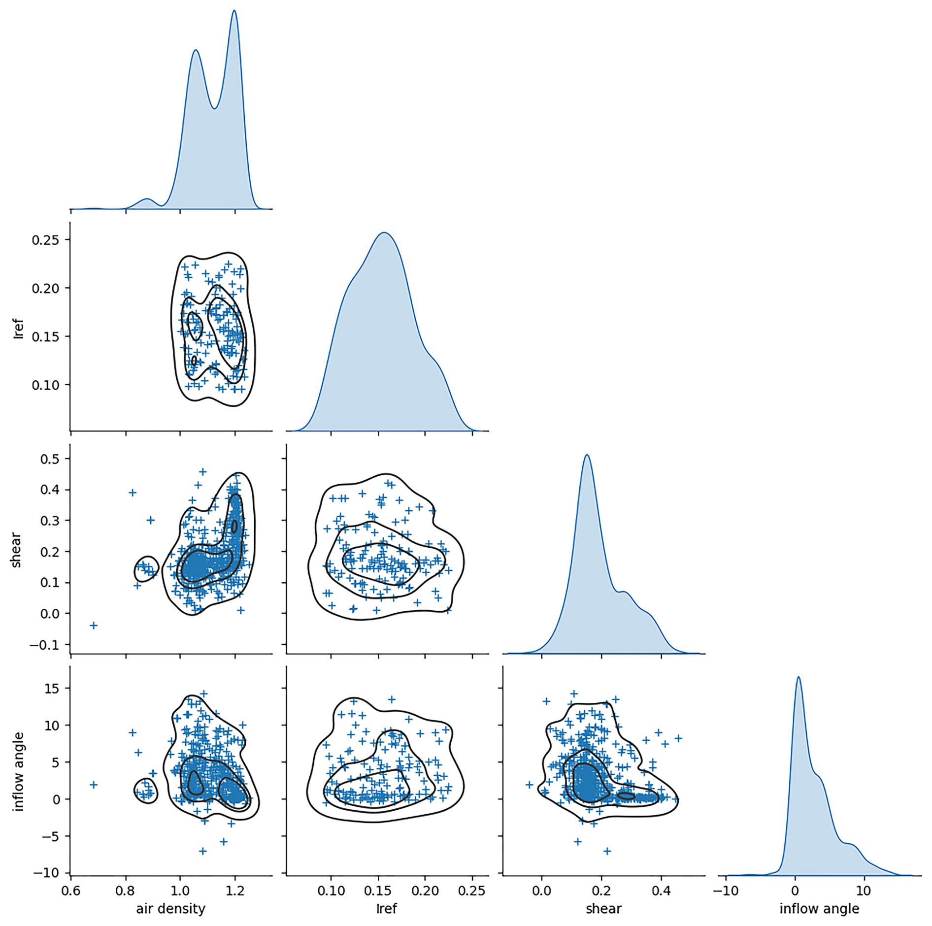
Figure 1 Scatter plots, density contour lines, and kernel density estimations for various wind condition parameters at a specific site. (+ indicates the measured values; the black lines represent contour lines, while those positioned along the diagonal indicate the kernel density of each wind parameter.)

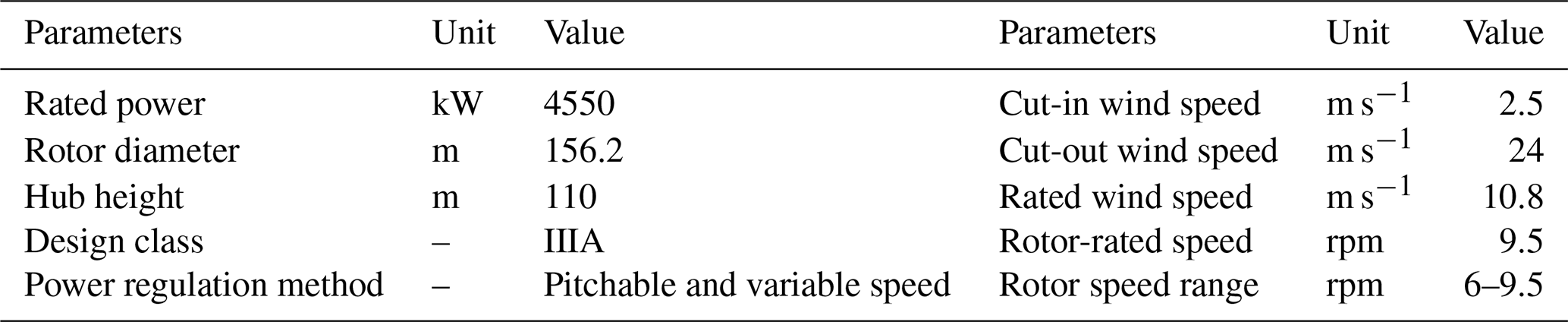
For specific wind parameters, simulations are conducted according to IEC standards for DLC 1.1 load cases, with a minimum duration of 10 min per time series. The resolution of wind speed is set at 2 m s⁻¹ intervals from cut-in to cut-out wind speed. A minimum of 15 simulations is required for each wind speed interval from (V_r–2 m s⁻¹) to cut-out (generally, 60 simulations are used), and six simulations are needed for each wind speed below (V_r–2 m s⁻¹). For WTG 156-4.55, with a cut-in wind speed of 2.5 m s⁻¹ and a cut-out wind speed of 24 m s⁻¹, at least 558 simulations are required.

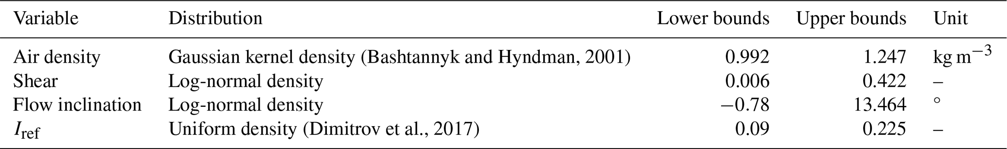
Aside from wind speed, the primary wind parameters affecting the loads on wind turbines include air density, turbulence intensity, wind shear, and flow inclination (Moriarty, 2008; Dimitrov et al., 2018; Kelly et al., 2014; Dimitrov et al., 2017). For the ranges and distributions of these variables, this study utilizes data from 541 meteorological towers in a specific region, with the lower boundary set at the first percentile and the upper boundary at the 99th percentile, as shown in Fig. 1.

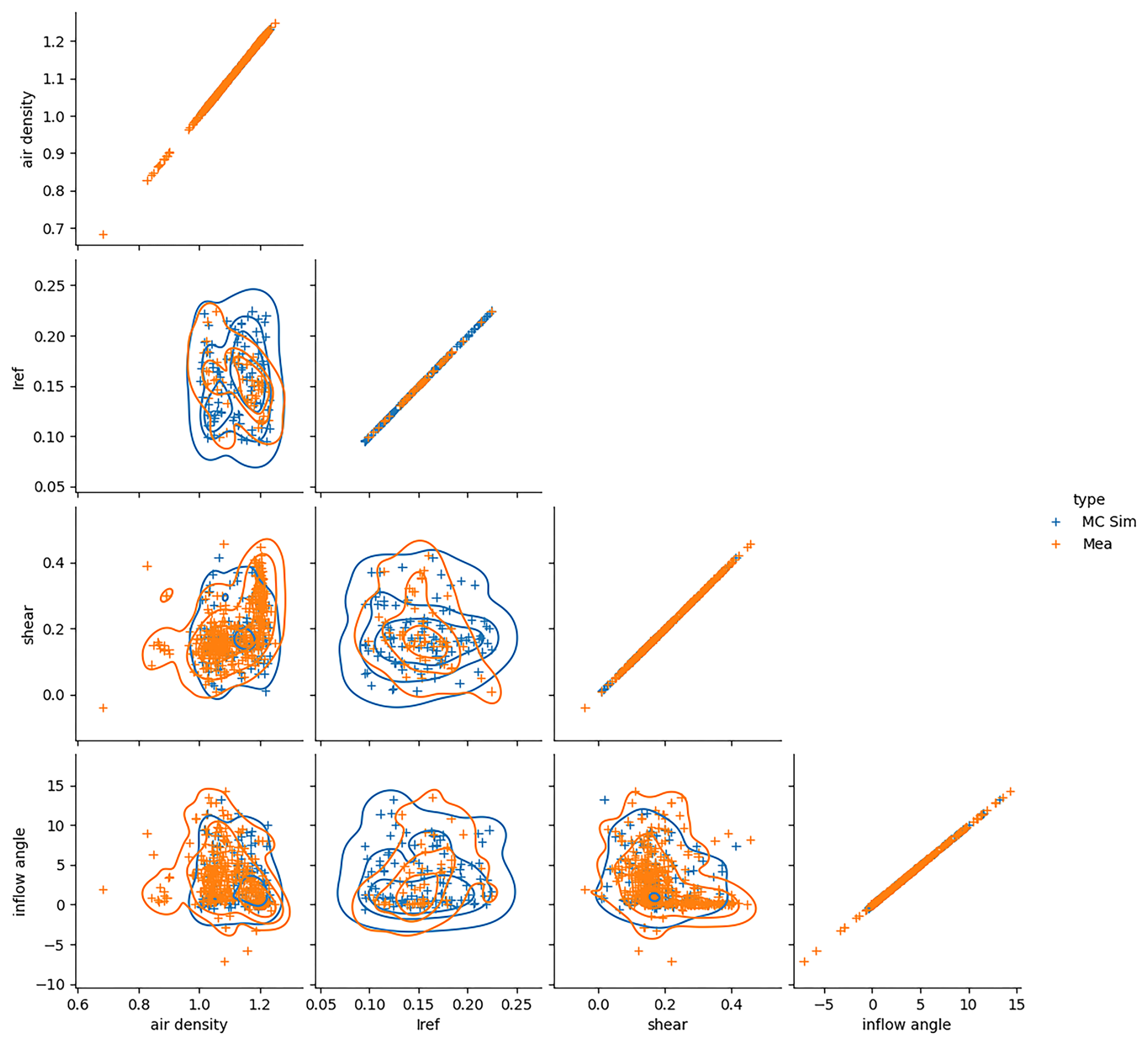
Figure 2 Scatter plots, density contour lines, and kernel density estimations for various wind condition parameters (blue dot indicates measured values, orange dot indicates MC sampled values; the solid lines represent contour lines, while the plots along the diagonal are scatter plots of the measured values versus the sampled values for each wind parameter).

Regarding turbulence intensity, this varies with different wind speeds. Equation (2) is used to calculate the turbulence intensity for each wind speed based on I_ref.

$$\begin{array}{}\text{(2)}& I_{V_i}={\displaystyle \frac{I_{\mathrm{ref}}\left(\mathrm{0.75}{V}_i+\mathrm{5.6}\right)}{V_i}}\end{array}$$

According to the distribution and range of various wind parameters in Table 1, the Monte Carlo sampling method was used for data collection, with a sample size of 100. As shown in Fig. 2, the statistical characteristics of the sampled data are basically consistent with those of the original data.

Table 1 Bounds of variation for the wind parameters considered. All values are defined as annual statistics.

The configuration of the wind turbine used in the simulation is shown in Table 2.

Table 2 The configuration of the wind turbine WTG156-4.55.

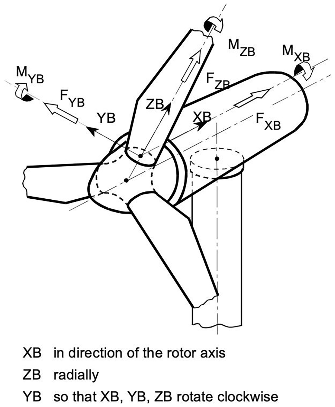
Using the Bladed software, a simulation was conducted for 558×100 normal operating conditions over a duration of 10 min each, generating a database for load extrapolation. In accordance with wind turbine design standards, the analysis of load extrapolation concerning the structural integrity must include at least the computation of extreme values for the blade root in-plane bending moment (IPBM), out-of-plane bending moment (OOPBM), and tip deflection, as shown in Fig. 3. The IPBM and OOPBM are described using the blade coordinate system from the Germanischer Lloyd Industrial Services GmbH (2012), as shown in Fig. 4. The M_YB is an out-of-plane bending moment and M_XB is an in-plane bending moment. This paper focuses on the methodological exposition, so the out-of-plane bending moment at the blade root will be analyzed as an example.

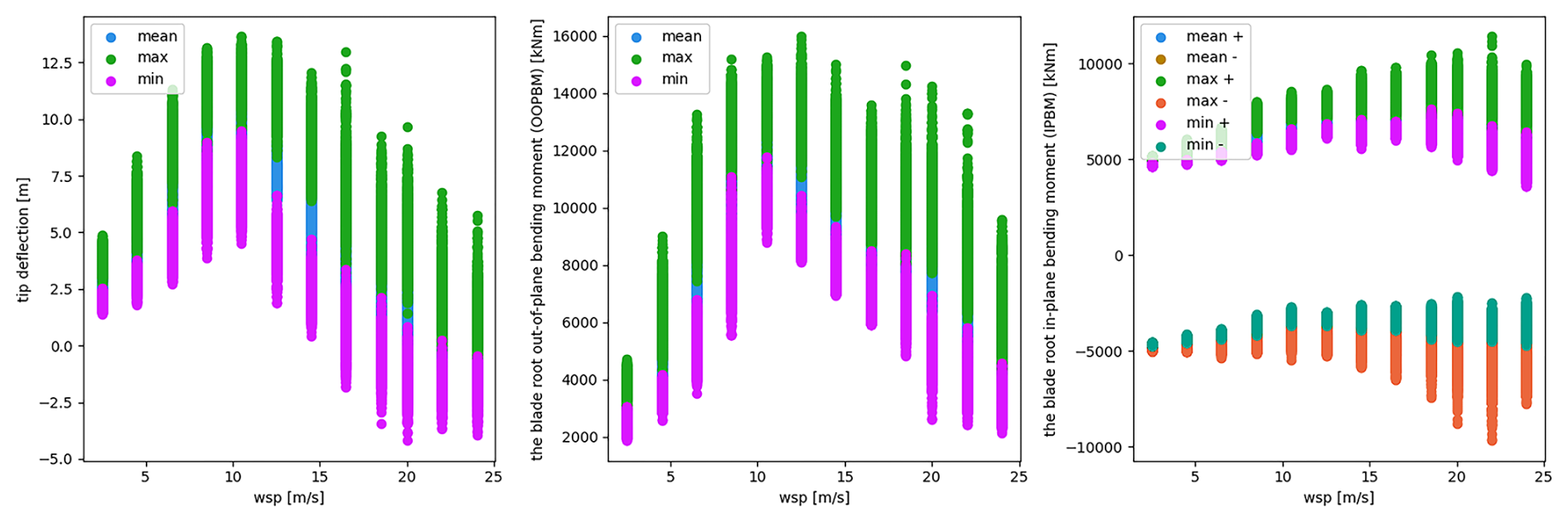
Figure 3 Basic statistical characteristic parameters under different wind speeds for sample: tip deflection (left), out-of-plane bending moment (OOPBM) (middle), and in-plane bending moment (IPBM) (right).

Figure 4 Coordinate system of wind turbine blade.

3 IEC standards recommend load extrapolation method

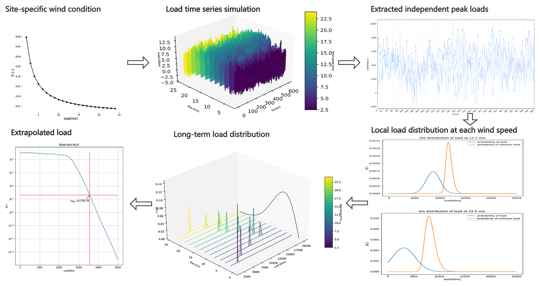
In accordance with IEC 61400-1:2019 and relevant literature, Fig. 5 illustrates the load extrapolation process adopted in this paper.

Figure 5 The benchmark method for the load extrapolation process.

The benchmark method utilized in this paper for load extrapolation at specific sites is outlined as follows:

1. The load time series simulation is run for different wind speeds, from cut-in to cut-out wind speeds, under normal power production conditions. This simulation is based on the site-specific wind parameters which include air density, turbulence intensity at different wind speeds, wind shear, and flow inclinations. A total of 558 simulated time series loads, each lasting 600 s, are produced when the wind speed interval is set at 2 m s⁻¹.

2. The “fitting before aggregation” method can be used to ascertain the long-term distribution of the extremes. The long-term distribution is derived by weighting these short-term distributions in accordance with the wind distribution, and the local peak distribution is fitted to the peaks at each wind speed.

3. Peaks are extracted from the load time series using the block maxima method. The 600 s time series is divided into 20 blocks, and each lasts 30 s. This block length is adequate to ensure the independence of the peaks, as detailed in Zhang et al. (2024).

4. The local peak distribution function of the extracted peak loads is fitted using the maximum likelihood method. The following is the probability density function (PDF) of the Weibull distribution:

   $$\begin{array}{}\text{(3)}& f\left(x;\mathit{\lambda },k,\mathit{\gamma }\right)={\displaystyle \frac{k}{\mathit{\lambda }}}{\left({\displaystyle \frac{x-\mathit{\gamma }}{\mathit{\lambda }}}\right)}^{k-\mathrm{1}}{e}^{-{\left(x-\mathit{\gamma }/\mathit{\lambda }\right)}^k},x\ge \mathit{\gamma },\end{array}$$

   where λ (scale parameter) controls the scale of the distribution, k (shape parameter) determines the shape of the distribution, and γ (location parameter) represents the threshold below which the probability density is zero.

   The extreme distribution for the maximum response L throughout the time interval [0,T] is obtained from the distribution of local peaks as follows:

   $$\begin{array}{}\text{(4)}& F_{\mathrm{extreme}}\left(L\mathrm{|}V\right)=F_{\mathrm{local}}{\left(L\mathrm{|}V\right)}^N,\end{array}$$

   where N is the expected number of independent peaks at the wind speed V during the time interval [0,T].

5. By integrating over the wind speeds, as described by the Rayleigh distribution, the extreme distribution can be used to derive the long-term distribution for the maximum response within the time interval [0,T].

   $$\begin{array}{}\text{(5)}& F_{\text{long-term}}\left(L\right)=\underset{v_{\text{cut-in}}}{\overset{v_{\text{cut-out}}}{\int }}{F}_{\mathrm{extreme}}\left(L\mathrm{|}V\right)f\left(V\right)\mathrm{d}V\end{array}$$

   and

   $$\begin{array}{}\text{(6)}& P\left(V\right)=\mathrm{1}-\exp \left[-\mathit{\pi }{\left({\displaystyle \frac{V}{\mathrm{2}{V}_{\mathrm{ave}}}}\right)}^{\mathrm{2}}\right],\end{array}$$

   where P(V) is the cumulative probability function, f(V) can be calculated, V is the wind speed, and V_ave is the average value of V.

6. The exceedance probability of the 50-year extreme load is estimated as follows:

   $$\begin{array}{}\text{(7)}& L_{\mathrm{50}\mathrm{year}}=F_{\text{long-term}}^{-\mathrm{1}}\left({\displaystyle \frac{\mathrm{1}}{\mathrm{50}\times \mathrm{365}\times \mathrm{24}\times \mathrm{6}}}\right).\end{array}$$

4 FastLE method

The standard extreme load extrapolation method was employed to simulate the load conditions for normal power production of the WTG156-4.55 turbine using Bladed 4.10.0.22. Each simulation took approximately 70 min. Utilizing a 32-core CPU as the computational resource, the total time required for the calculations would be around 20.344 h. In wind farms containing several, dozens, or even hundreds of turbines, the time-intensive nature and substantial computational resource demands of this approach are clearly impractical. Consequently, overly conservative designs are often employed, which reduce the economic viability of projects. To address these challenges, this paper introduces a rapid extrapolation method for extreme loads, utilizing a load distribution meta-model called FastLE.

4.1 Independence testing

As we all know, ensuring that block maxima chosen from each time series are independent of each other is crucial for the statistical extrapolation method. Blum et al.'s (1961) test has been applied to wind turbine load extrapolation by Fogle et al. (2008). It was discovered that block sizes of approximately 10–15 s for OOPBM produced independent block maxima when evaluated at the 1 % significance level using a statistical test.

To balance the large number of data needed to fit the local load distribution with the requirement to reduce sample numbers for maintaining independence, we introduce DcorrX (cross distance correlation) as an additional test for independence (Shen et al., 2024). DcorrX is an independence test between two time series, where the population parameter equals zero if and only if the time series are independent. This method is grounded in the concept of energy distance between distributions.

Let x and y be (n,p) and (n,q) series, respectively, which each contain y observations of the series X_t and Y_t. Similarly, let x[j:n] be the $\left(n-j,p\right)$ last n−j observations of x. Let $y\left[\mathrm{0}:\left(n-j\right)\right]$ be the $\left(n-j,p\right)$ first n−j observations of y. Let M be the maximum lag hyperparameter. The cross distance correlation is defined as follows:

$$\begin{array}{}\text{(8)}& {\displaystyle }{\mathrm{\text{DcorrX}}}_n\left(x,y\right)=\sum _{j=\mathrm{0}}^M{\displaystyle \frac{n-j}{n}}{\text{Dcorr}}_n\left(x\left[j:n\right],y\left[\mathrm{0}:\left(n-j\right)\right]\right),\text{(9)}& {\displaystyle }{\text{Dcorr}}_n\left(x,y\right)={\displaystyle \frac{{\text{Dcov}}_n\left(x,y\right)}{\sqrt{{\text{Dcov}}_n\left(x,x\right)\cdot {\text{Dcov}}_n\left(y,y\right)}}},\text{(10)}& {\displaystyle }{\text{Dcov}}_n\left(x,y\right)={\displaystyle \frac{\mathrm{1}}{n\left(n-\mathrm{3}\right)}}tr\left(C^x{C}^y\right),\text{(11)}& {\displaystyle }\begin{array}{rl}{C}_{ij}^x& =\left[D_{ij}^x-{\displaystyle \frac{\mathrm{1}}{n-\mathrm{2}}}\sum _{t=\mathrm{1}}^n{D}_{it}^x-{\displaystyle \frac{\mathrm{1}}{n-\mathrm{2}}}\sum _{s=\mathrm{1}}^n{D}_{sj}^x+\right.\\ & \left.{\displaystyle \frac{\mathrm{1}}{\left(n-\mathrm{1}\right)\left(n-\mathrm{2}\right)}}\sum _{s,t=\mathrm{1}}^n{D}_{st}^x\right]{\mathrm{1}}_{i\ne j},\end{array}\end{array}$$

where $D_{ij}^x$ and $D_{ij}^y$ represent the distance between the ith and jth observations in samples x and y.

Similar to other independence tests, p values are employed to represent the statistical probability under the premise that two variables are independent (the population parameter equals zero), serving as evidence for the mutual independence between the variables.

For a total of 55 800 samples collected under normal power production conditions, the data were categorized into three types based on wind speed: the full wind speed range, low wind speed (≤10 m s⁻¹), and high wind speed (> 10 m s⁻¹). The independence of these three sample groups was assessed using DcorrX. As illustrated in Fig. 6, with a block size of 30 s, 74.65 % of the overall samples was found to be independent, 61.1 % of the low wind speed samples was independent, and 84.33 % of the high wind speed samples was independent. It is widely recognized that lower wind speeds contribute minimally to the tails of long-term load distributions (Fogle et al., 2008). Consequently, increasing the block size to guarantee independence at these low wind speeds does not aid in achieving our ultimate objective of statistical load extrapolation. Based on the test results, the final block size was selected to be 30 s, which ensures that the majority of load peaks are independent.

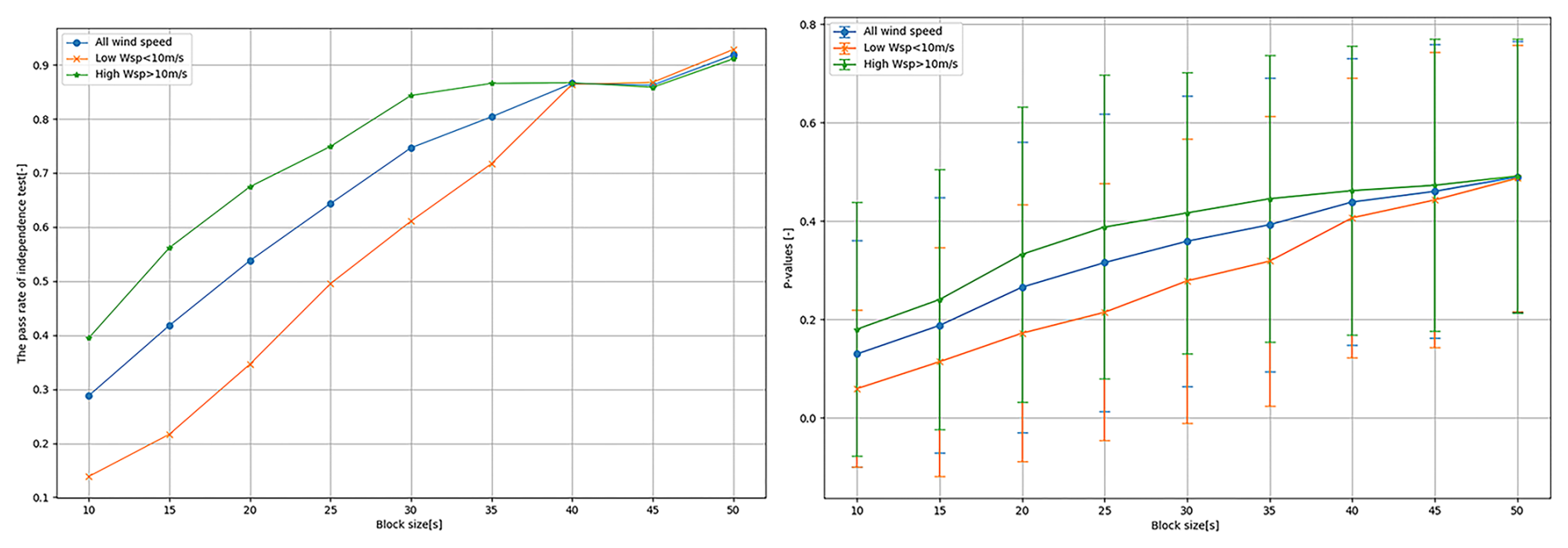
Figure 6 The pass rates (left) and p values (right) for the DcorrX test under different block sizes. The blue color represents the full wind speed range, while orange and green denote the low and high wind speed.

4.2 Local load distribution fitting model selection

The local peak distribution function of extracted peak loads is typically modeled using a Weibull distribution (Fogle et al., 2008; Yang et al., 2022). However, normal, log-normal, and Gumbel distributions are also employed in fitting load distributions. Due to the varying dynamic effects of wind turbines, the distribution of peak loads can vary at different wind speeds, as illustrated in Fig. 7.

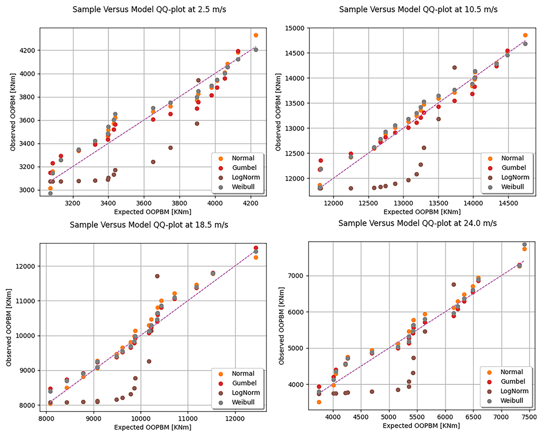
Figure 7 QQ-plots (quantile-quantile plots) of the peak loads under different wind speeds and different distributions. The orange points denote the normal distribution, the red points represent the Gumbel distribution, the brown points indicate the log-normal distribution, and the gray points correspond to the Weibull distribution. The dashed line represents y=x.

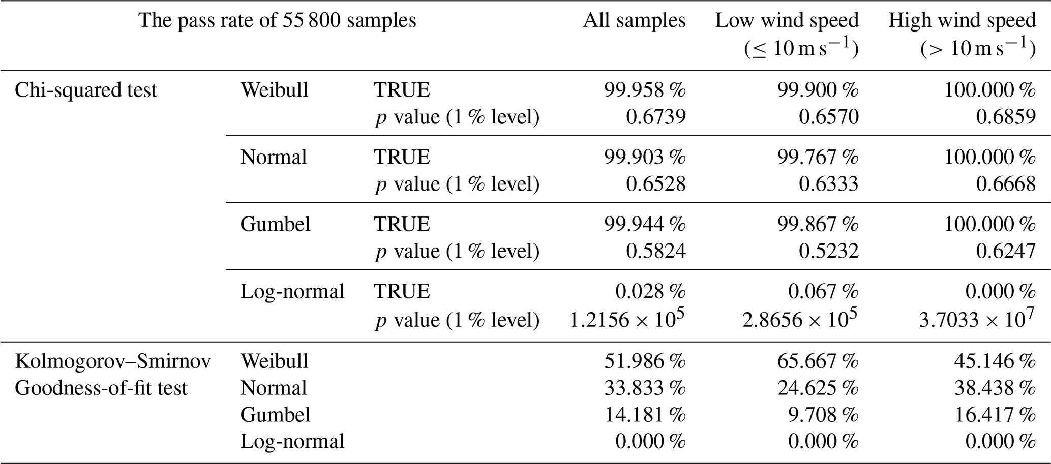
The quality of the load distribution fitting is critical for the extrapolation of extreme loads. In this study, the extracted peak loads from 55 800 normal power production conditions, with a block size of 30 s, are fitted using the maximum likelihood method to Weibull, normal, Gumbel, and log-normal distributions to determine their respective parameters. A chi-squared test (Burnham and Anderson, 2002) is then performed to validate these fits. The optimal model is selected based on the Kolmogorov–Smirnov (Dixon, and Massey Jr., 1983) goodness-of-fit test. The results are detailed in Table 3.

Table 3 The result of the chi-squared test and the Kolmogorov–Smirnov goodness-of-fit test for different distributions.

4.3 Local load distribution meta-model

4.3.1 Issue statement

In the process of extreme load extrapolation, simulating load time series for wind turbine normal operating conditions is the most computationally intensive and time-consuming step. To effectively speed up the load extrapolation, this study references certain literature to introduce wind parameters into the meta-model for load components (Dimitrov et al., 2018; Graf et al., 2016). The introduction of the meta-model for load extrapolation can be implemented in the following three ways, as illustrated in Fig. 8.

For option A, this paper limits the overall training samples to just 100 due to the significant computational resources required. The most critical drawback is that the turbulence intensity at various wind speeds for specific sites does not fully align with the model defined in the IEC standards (Eq. 2). This discrepancy necessitates including turbulence intensities at different wind speeds as inputs, which substantially increase the model's input dimensions. To adequately cover a sufficient range of wind parameters, the total number of samples would need to be expanded, thereby presenting a limitation to this option. For option B, the training dataset comprises a total of 55 800 sub-condition samples. While this is suitable for the meta-model overall, it leads to an increase in the output dimensions of the meta-model. With a block size of 30 s, the output variables for a single wind speed amount to 20 dimensions (for a 600 s load time series). Furthermore, the order of these dimensions does not affect the results, resulting in convergence issues during model training. Given the limitations in sample size and input/output dimensions, this paper chooses option C. The training samples employ wind parameters from sub-conditions, and the output comprises the parameters of the Weibull distribution corresponding to each wind speed.

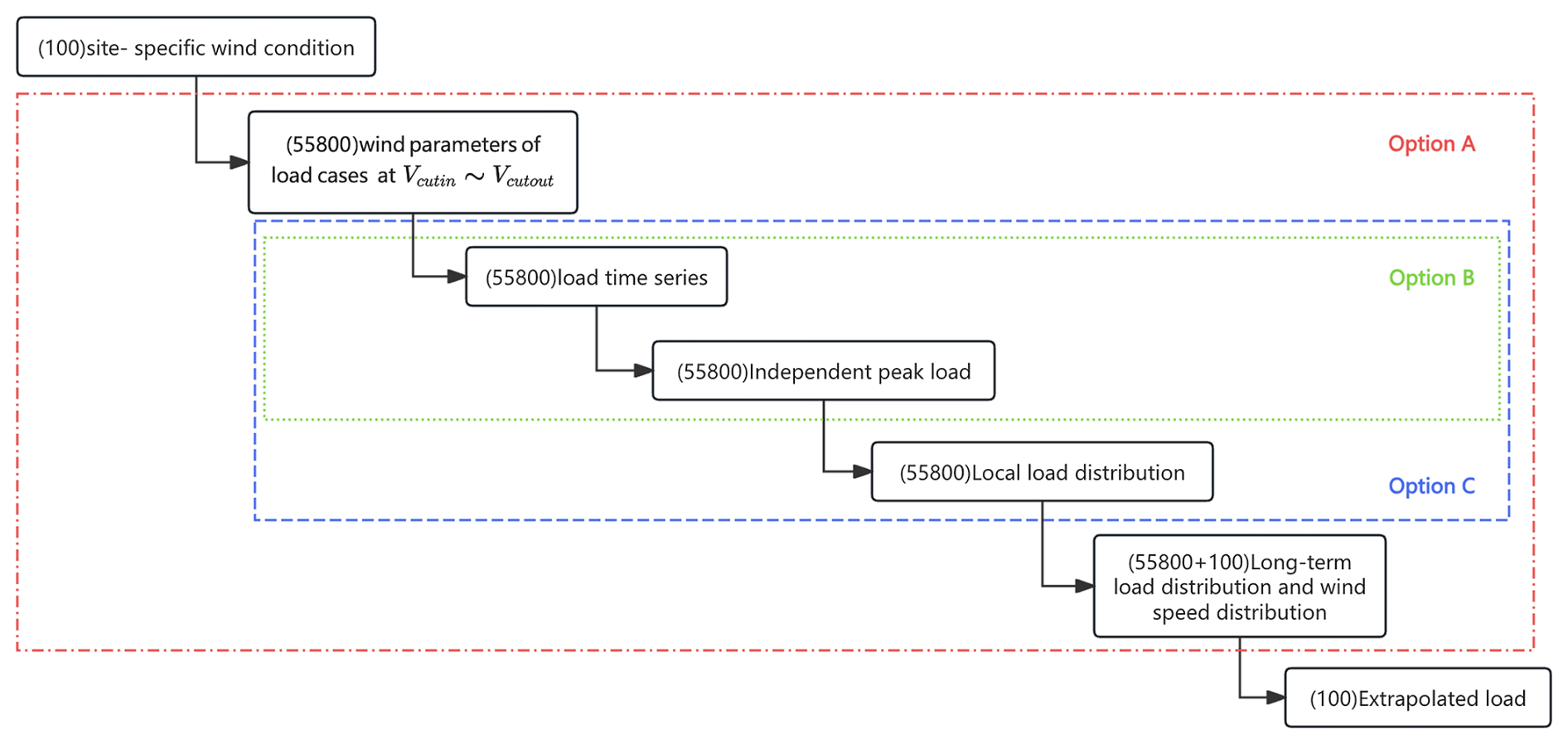
Figure 8 Schematic diagram of the three ways to implement a meta-model for load extrapolation. The dashed red, green, and blue boxes represent the scopes of option A, B, and C, respectively. The numbers in square brackets indicate the number of samples.

4.3.2 Multi-layer perceptron

In this paper, we employ a multi-layer perceptron (MLP) regression model to construct the meta-model. The MLP is a supervised learning algorithm designed to learn a mapping function $f:R^m\to R^o$ from a dataset, where m represents the number of input dimensions and o represents the number of output dimensions. Given a feature set X=x₁x₂x_m and a target variable y, the MLP can model complex non-linear relationships for tasks such as regression. However, the MLP has certain disadvantages, which include the fact that MLPs with hidden layers have a non-convex loss function, leading to multiple local minima. This means that different random weight initializations can result in varying validation accuracies. Additionally, MLPs require the tuning of several hyperparameters, such as the number of hidden neurons, the number of layers, and the number of iterations.

The input of the local peak distribution meta-model includes wind speed, its corresponding turbulence intensity, wind shear, air density, inflow angle, and yaw misalignment (configured according to the IEC standard with values of −8, 0, and 8°). The output comprises the shape parameter and scale parameter of the Weibull distribution (with the location parameter set to 0). Additionally, normalization is applied based on the training samples, using the method shown in the following equation:

$$\begin{array}{}\text{(12)}& z={\displaystyle \frac{x-\mathit{\mu }}{\mathit{\sigma }}},\end{array}$$

where μ is the mean of the training samples and σ is the standard deviation of the training samples.

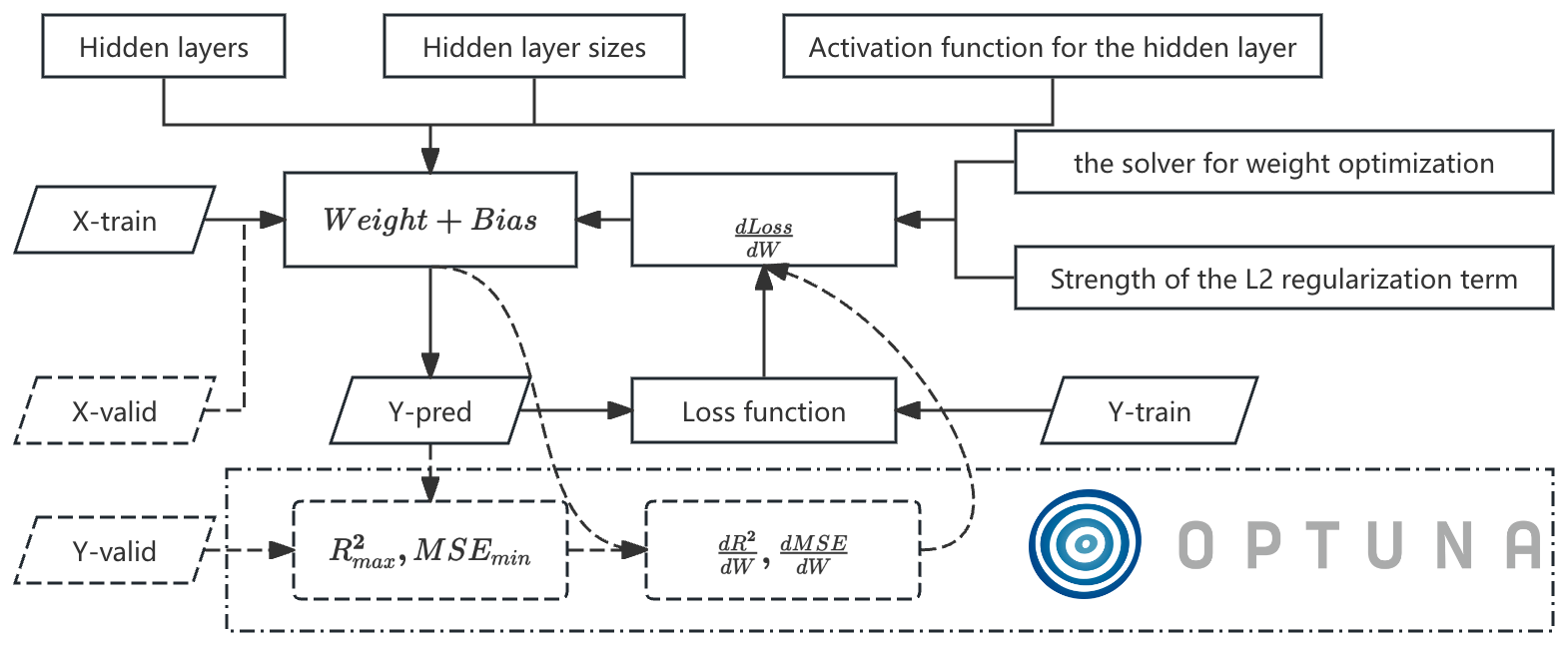
Figure 9 The workflow of model training with the Optuna optimization framework. The logo is from https://optuna.org/ (last access: 15 October 2025).

4.3.3 Model training with the Optuna optimization framework

Due to the need for hyperparameter tuning during MLP model training, several variables are essential to improving the model's regression performance. These include the number of hidden layers, the size of each hidden layer, the activation function used for the hidden layers, the solver for weight optimization, and the strength of the L2 regularization term, among others. To enable effective hyperparameter tuning and optimization, this paper introduces Optuna (Akiba et al., 2019), an open-source framework that automates the search for optimal parameters. The workflow is illustrated in Fig. 9.

We employed 1440 validation samples and utilized Optuna for the optimization of two objectives: minimizing mean squared error (MSE) (objective 0) and maximizing R² (objective 1). After 1000 iterations, the trends of both objective functions demonstrated consistent behavior, as shown in Fig. 10.

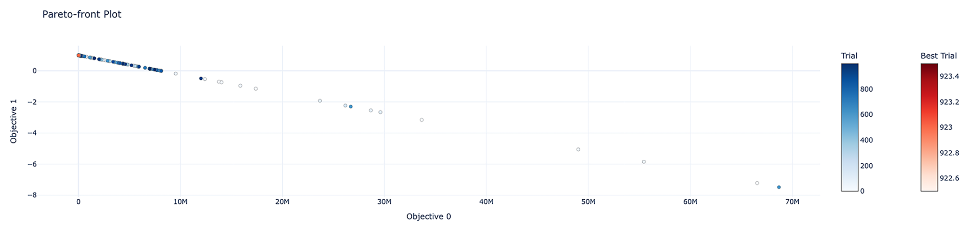
Figure 10 Pareto-front plot for the training of a dual-objective model (objective 0: MSE and objective 1: R²).

After optimization, the final optimal MLP regression model was configured with three hidden layers comprising 42, 188, and 125 neurons, respectively. The ReLU activation function was used, and the solver chosen was L-BFGS. A detailed analysis of the significance of these hyperparameters in the MLP regression task is presented in Fig. 11, which highlights the activation function as the most critical factor.

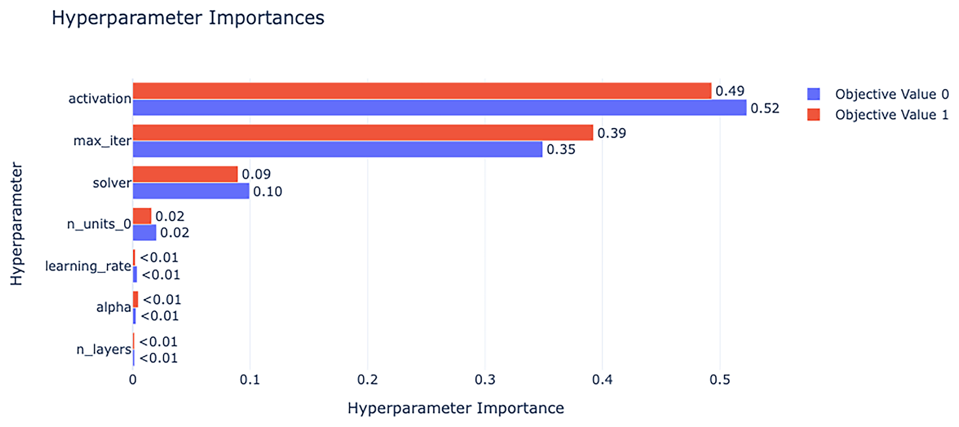
Figure 11 Analysis of hyperparameter significance for local load distribution meta-model (objective 0: MSE and objective 1: R²).

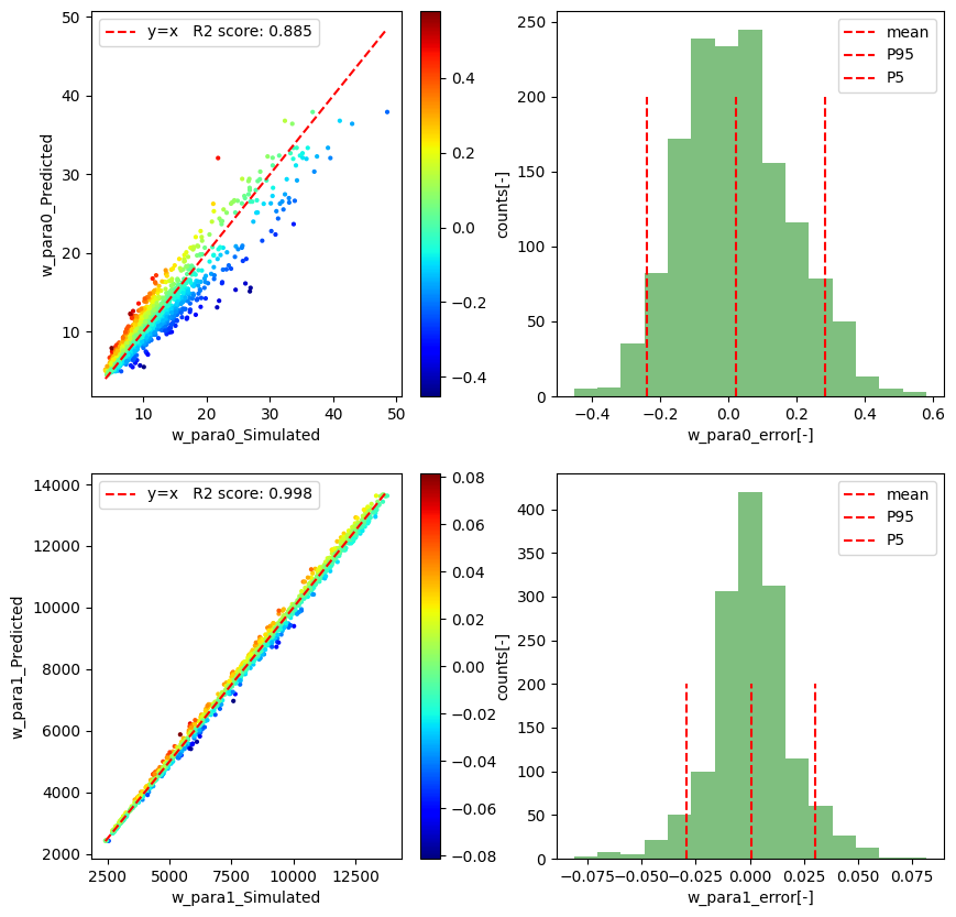
The performance of the optimal model on the validation sample is illustrated in Fig. 12. As there is no significant offset in the data, the location parameter gamma is set to 0 for the Weibull distribution. For the shape parameter (denoted as w_para0 in the figure), the R² between the true and predicted values is 0.885, with a 90 % confidence interval for the error (the error is defined as error = (predicted value − actual value) $/$ actual value) ranging from −0.22 to 0.23. For the scale parameter (denoted as w_para1 in the figure), the R² is 0.998, with a 90 % confidence interval for the error ranging from −0.028 to 0.028.

Figure 12 The performance of the optimal model on the validation sample.

4.4 Post-processing

As shown in Fig. 13, for site-specific wind conditions, a detailed description of the interval from V_cut-in to V_cut−out with a 2 m s⁻¹ interval is provided. For any given wind speed V_i, the corresponding turbulence intensity TI_i, wind shear α_i, and flow inclination I_i are used as inputs for the local load distribution meta-model. This allows us to obtain the parameters for the local load peak Weibull distribution at that wind speed. Using Eq. (4), the extreme distribution can be derived. Subsequently, based on all wind speeds' extreme distributions and the Weibull probability density function, Eq. (5) is applied to determine the long-term load distribution for the site. Finally, using Eq. (6), the extrapolated load for a 50-year return period is calculated.

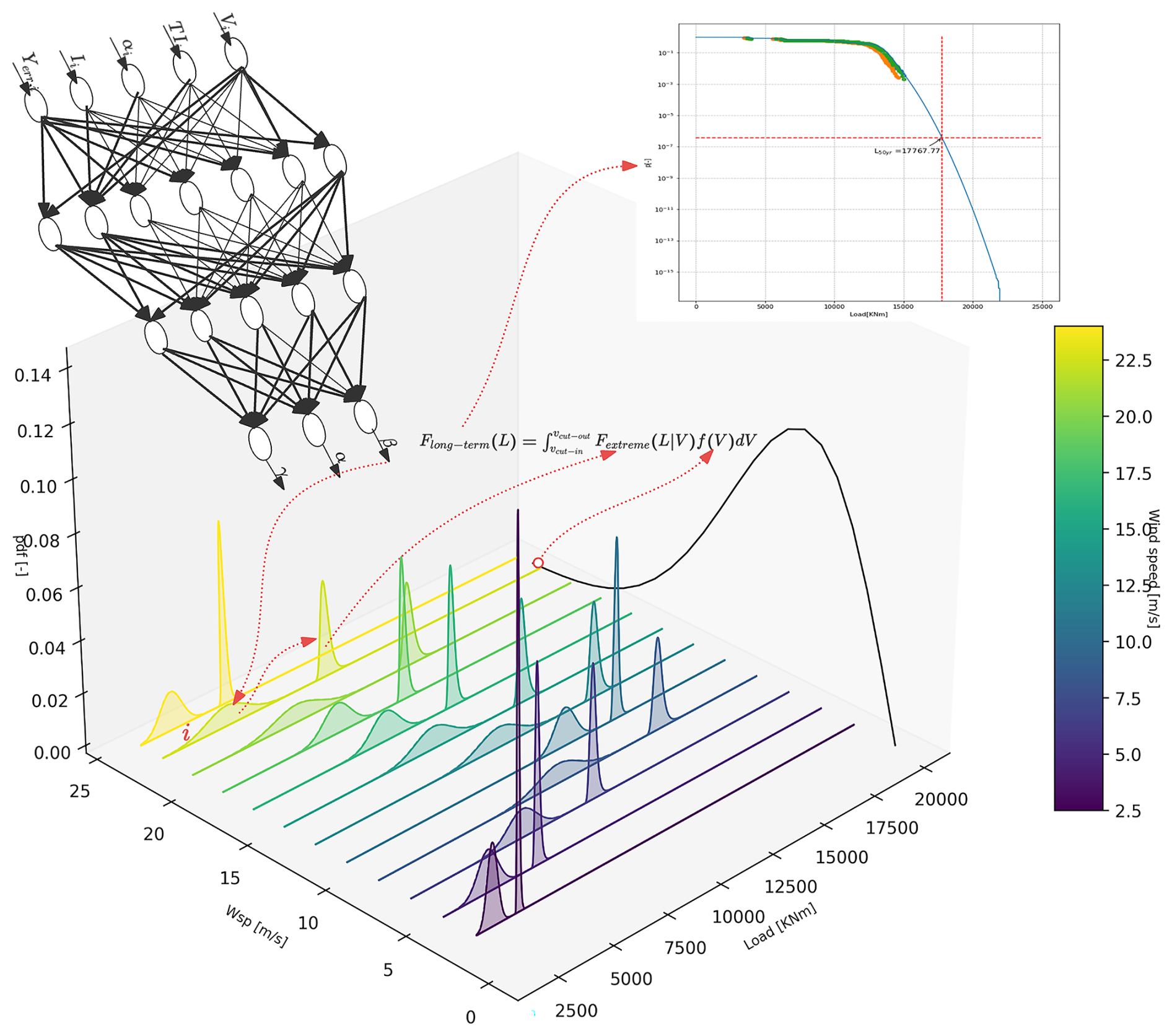
Figure 13 Schematic diagram of the FastLE post-processing. The dashed arrows indicate the post-processing steps, the solid black line represents the probability density distribution of wind speed, and the different-colored shaded areas represent the load distributions at different wind speeds.

4.5 The framework of FastLE

Integrating the content from all sections in this chapter forms a load extrapolation method based on the load distribution meta-model, whose overall framework is shown in Fig. 14.

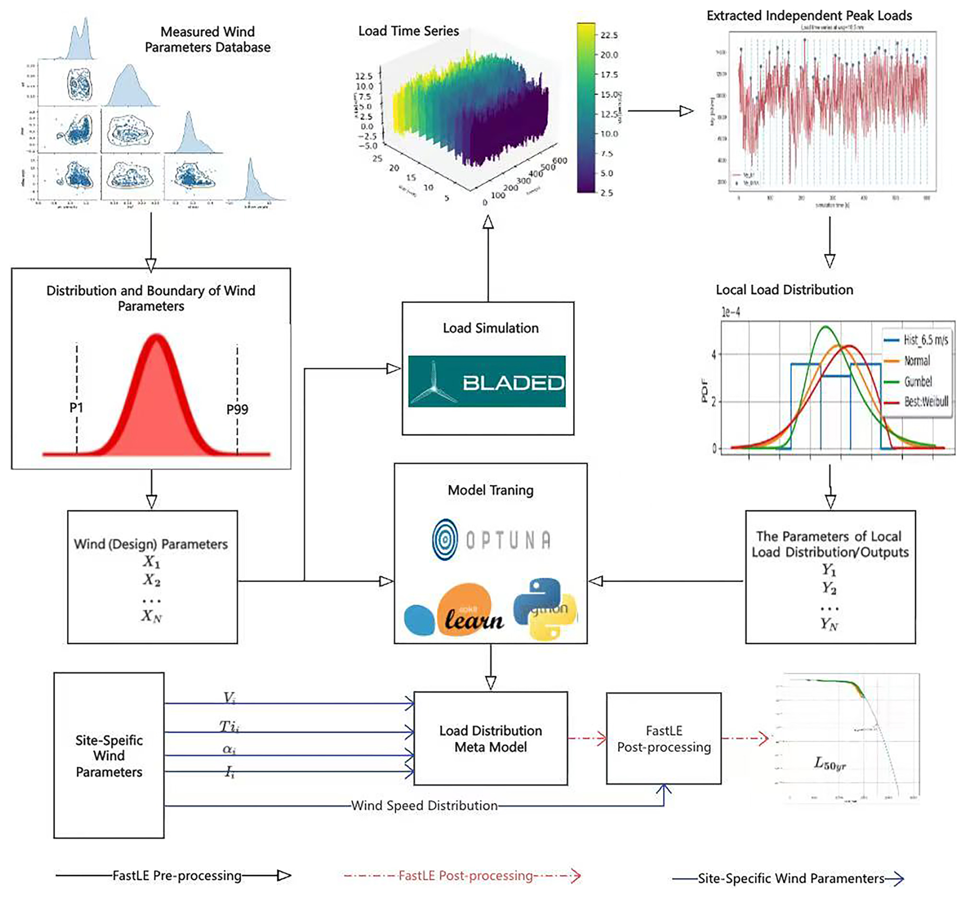
Figure 14 The framework of FastLE. The solid black lines denote pre-processing, the dashed red lines represent post-processing, and the solid blue lines indicate the site-specific application. The logo is from https://scikit-learn.org (last access: 15 October 2025), https://www.dnv.com/software/services/bladed/ (last access: 15 October 2025), https://optuna.org/ (last access: 15 October 2025), https://www.python.org/ (last access: 15 October 2025).

5 Test case

FastLE is designed to assess the structural integrity of wind turbines during the design phase of a wind farm and does not involve measuring load data. Therefore, the test case in this paper utilizes the Monte Carlo sampling method to generate 20 sets of wind parameters, based on their respective ranges and distributions. To distinguish them from the earlier 100 training and validation datasets, the test case numbers begin at 101, as illustrated in Table 4. The turbine model used is WTG156-4.55, configured with the Bladed 4.10.0.22 software as detailed in Table 5 to simulate the OOPBM under normal operating conditions. Following this simulation, a load extrapolation was conducted to estimate conditions for a 50-year return period.

Table 4 Wind parameter table for 20 test cases based on Monte Carlo sampling.

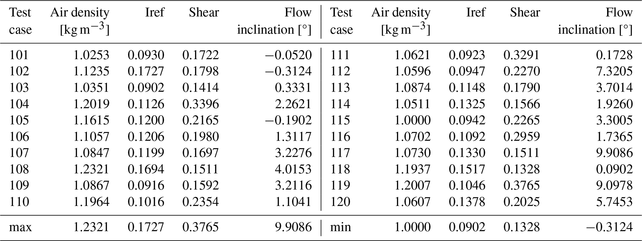
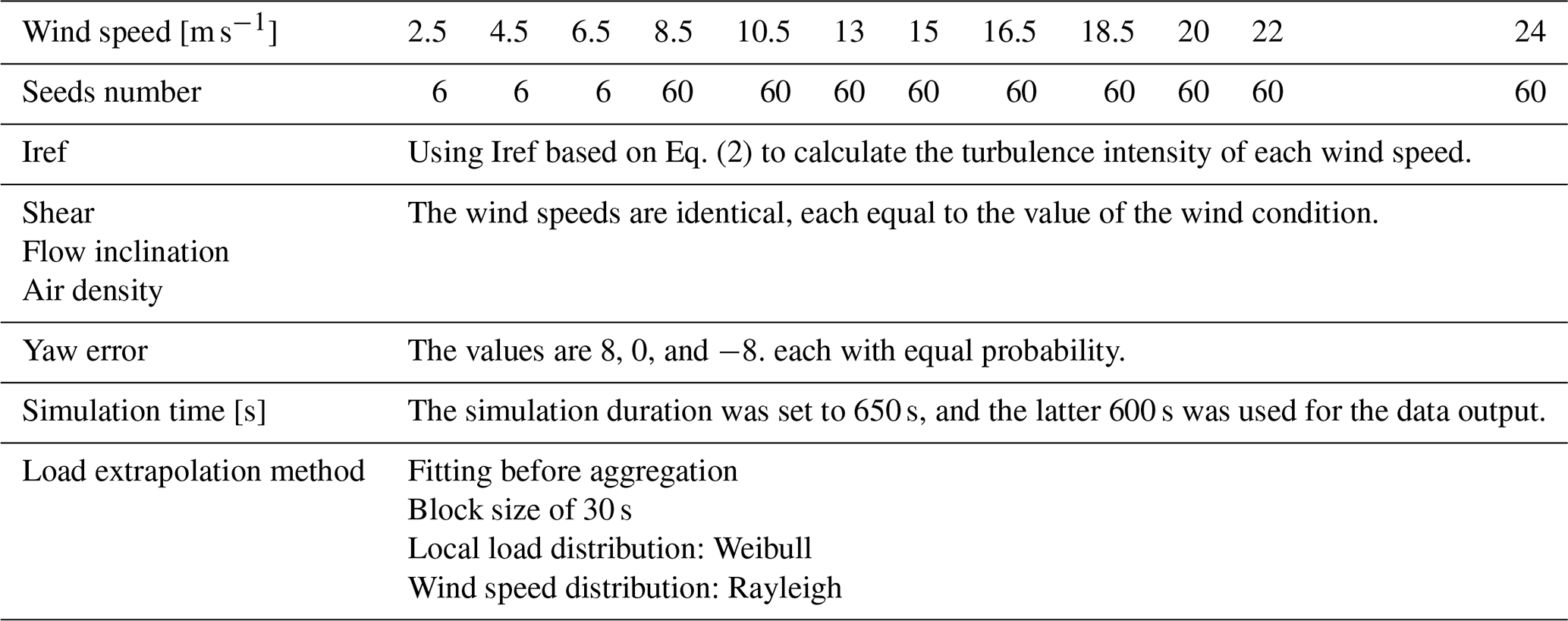
Table 5 Load simulation and load extrapolation configuration table.

Assuming all test cases employ the same wind speed probability density, modeled as a Weibull distribution with parameters A=8.463 and k=2, the results for one of the test cases are depicted in Fig. 15.

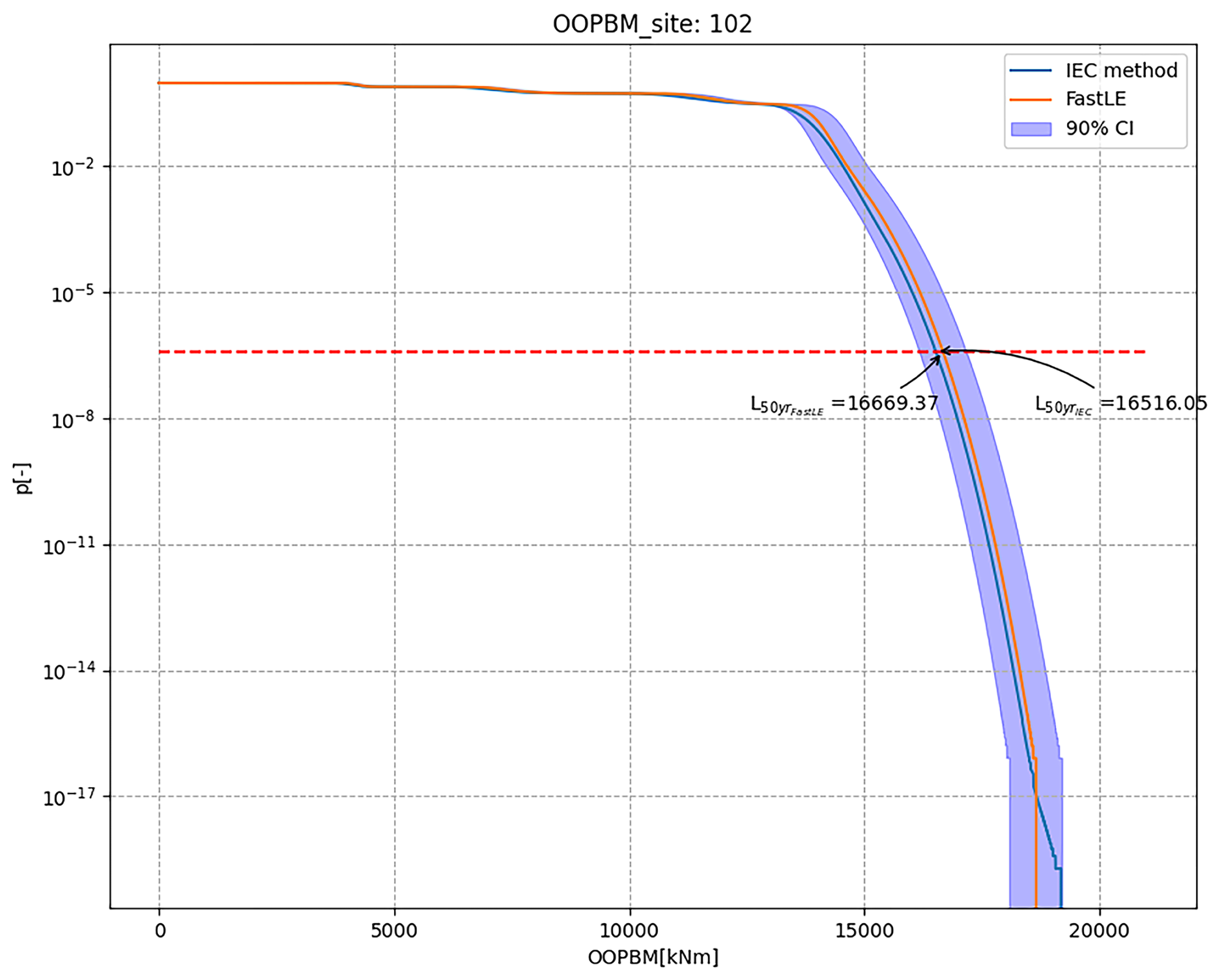
Figure 15 Load extrapolation results for test case 102. The solid blue line represents the IEC method, the red line denotes the FastLE method, the shaded area indicates the 90 % confidence interval, and the dashed red line corresponds to the probability of $\mathrm{3.8}\times {\mathrm{10}}^{-\mathrm{7}}$.

For all test cases, the 50-year return period extrapolated loads for the OOPBM calculated using the FastLE method were compared to those derived from the IEC method, as illustrated in Fig. 16. The absolute percentage error (APE) ranges from 0.421 % to 6.818 %, with an average of 3.165 %. When utilizing the P95 results from FastLE, the APE range narrows to between 0.326 % and 4.288 %, with an average of 2.22 %. The entire process using the IEC standard method requires approximately 400 h (20 test cases ⋅20.344 h, 32 core CPU) solely for load simulation, whereas the complete process with FastLE takes only seconds. The results demonstrate that FastLE can maintain high computational accuracy while achieving the extrapolation of extreme loads for wind turbines in seconds. This capability can be used for structural integrity assessments of wind turbines under different wind resources and for optimizing wind farm designs with extrapolated loads as constraints. Of course, the simulation time required to generate the database for FastLE is approximately 2000 h (on a 32-core CPU). However, this essentially accomplishes a compression of the timeline via FastLE, thereby facilitating the rapid iteration of design solutions for specific sites.

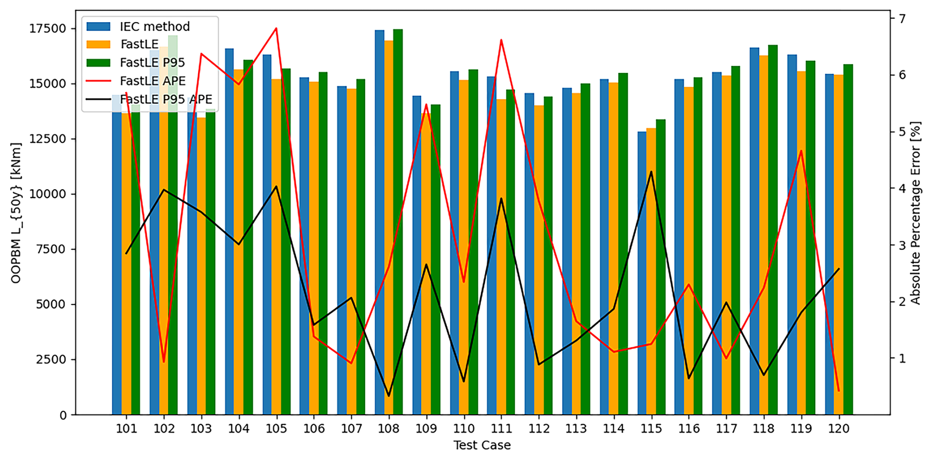
Figure 16 The load extrapolation results using the FastLE and IEC methods for 20 test cases. The blue bars represent the load extrapolation results from the IEC method, the orange bars denote those from FastLE, and the green bars indicate the load extrapolation results at the 95th percentile of FastLE. The solid red line represents the APE of the FastLE results compared to the IEC results.

6 Discussion and conclusion

6.1 Discussion

This paper introduces FastLE, a load distribution meta-model method specifically designed for site-specific load extrapolation. This innovative approach enables the rapid and accurate calculation of 50-year return period extrapolated loads for various turbine locations in a wind farm, doing so in mere seconds. Utilizing the WTG155-4.55 model with an out-of-plane bending moment (OOPBM) load component, FastLE dramatically reduces the simulation time for load extrapolation from 20 h to just seconds, while maintaining an average absolute percentage error (APE) of only 3.165 %. This advancement makes it feasible to incorporate extrapolated loads as constraints in wind farm optimization design, thereby ensuring the structural integrity of wind turbines at specific sites.

The process of load extrapolation for wind turbines consists of numerous steps, each with multiple implementation approaches. Taking “fitting before aggregation” as an example, peaks are extracted from the time series using three methods: global maxima, block maxima, and peak over threshold. Various distributions have been applied to these extracted peaks, including local load distribution functions such as the Weibull, normal, Rayleigh, and Gumbel distributions. Different approaches, methods, and parameters can all affect the extrapolated load. Based on relevant literature, this paper selects the recommended optimal path, which includes using a block size of 30 s, block maxima, and a Weibull distribution. The study primarily investigates the feasibility of a rapid extrapolation method for extreme loads and does not perform a systematic analysis of importance or parameter sensitivity. During the selection process for the optimal local peak distribution, the Kolmogorov–Smirnov goodness-of-fit test was employed for ranking the options. The Weibull distribution emerged with the highest optimal proportion at 51.986 %, significantly surpassing other distributions. However, the normal distribution also showed a substantial optimal proportion of 33.833 %, and the Gumbel distribution accounted for 14.181 %. This suggests that the optimal distribution for specific wind speeds may not always be the Weibull distribution. Nevertheless, due to the lack of a more suitable method at present, the Weibull distribution was predominantly applied across all wind speeds. This approach could potentially introduce errors into subsequent load extrapolations. Furthermore, in analyzing the discrepancies in the extrapolated OOPBM loads for test case 101, it was discovered that the Weibull distribution was not optimal for certain wind speeds. This finding validates the aforementioned point, as illustrated in Fig. 17. Additionally, inspired by the International Electrotechnical Commission (2019), local peak distributions at various wind speeds can be represented using a Gaussian mixture model, which combines multiple Gaussian distributions with different weights. This approach offers a viable avenue for further research in the field.

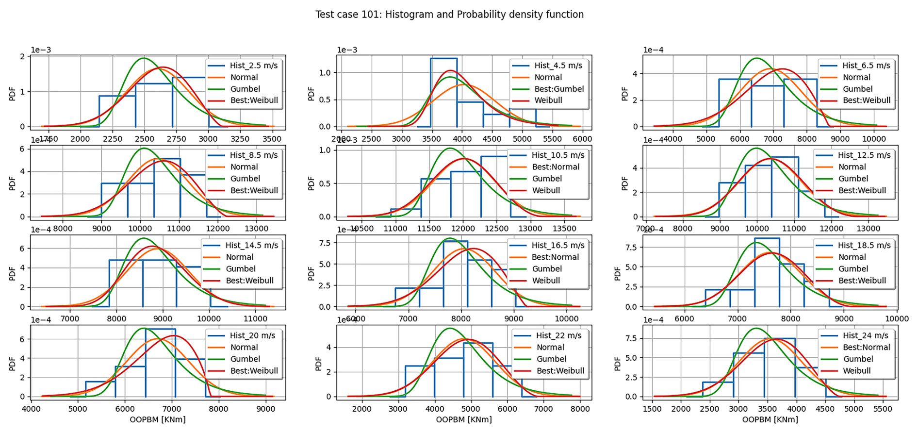
Figure 17 Optimal local load distributions under different wind speeds for test case 101. The blue histogram represents the load statistics at the current wind speed, the orange line denotes the normal distribution fit, the green line represents the Gumbel distribution fit, and the red line indicates the Weibull distribution fit.

Another crucial issue is the uncertainty analysis of FastLE. Load extrapolation is fundamentally probabilistic, and its implementation involves several factors that contribute to uncertainty in the results. These factors include the number of load simulation seeds, the methods used for selecting and testing independent samples, the determination of the optimal distribution, and, notably, the training of local peak distribution parameters within the meta-model. As an example, in the meta-model training process for the local load distribution parameters in test case 106, the uncertainty can influence both the local load distribution and the extreme load distribution, as demonstrated in Fig. 18, ultimately affecting the load extrapolation results. However, the manner in which these disturbances propagate during the load extrapolation process remains unknown. Related investigations are ongoing, and although this paper does not yet address this aspect, it is undeniable that this issue is of critical importance.

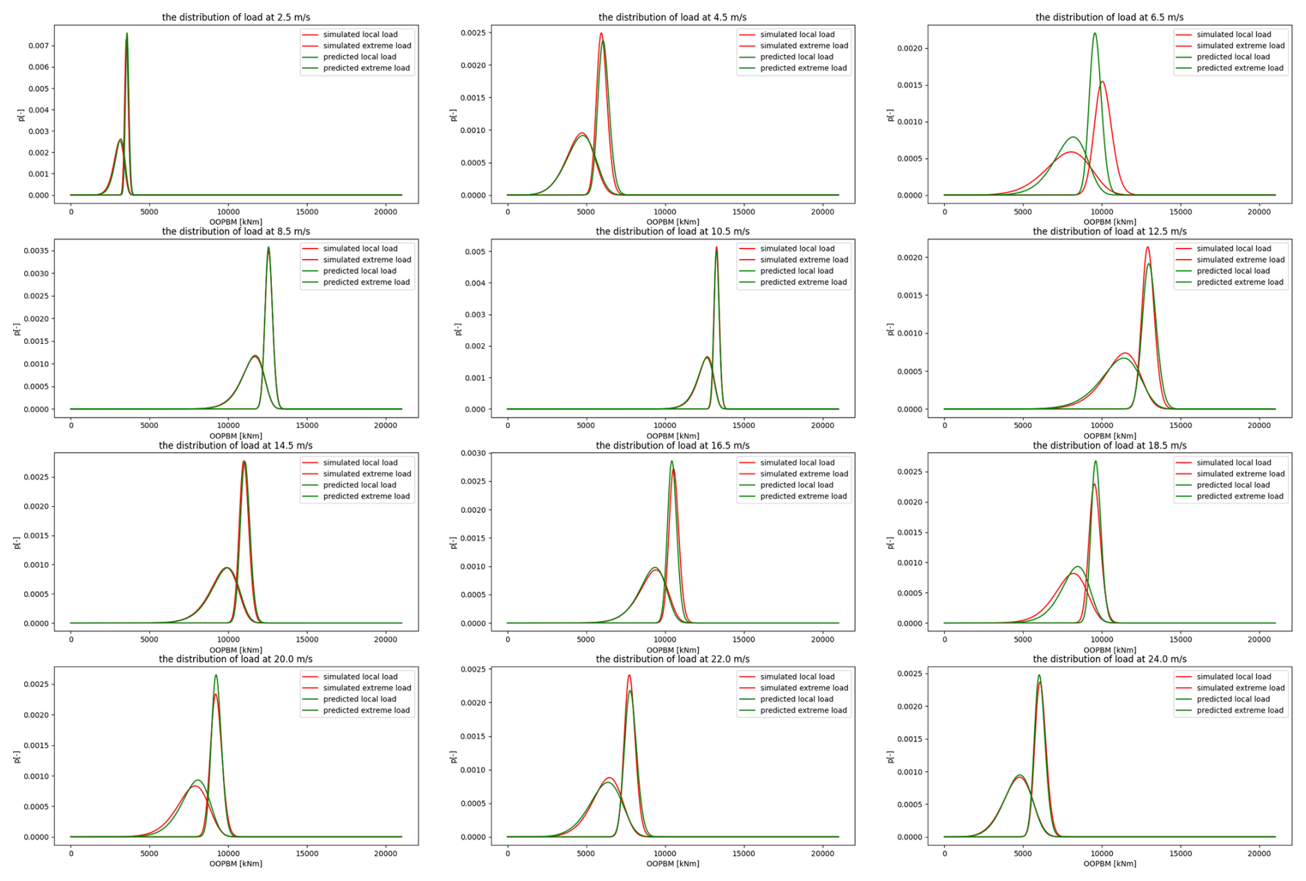
Figure 18 Local load distributions and extreme load distributions derived from the meta-model and simulated data fitting at various wind speeds for test case 106. Red denotes the simulated values, while green represents the predicted values.

6.2 Conclusion

This paper introduces FastLE, a rapid load extrapolation method based on meta-models and tailored to specific site conditions. By leveraging extensive historical statistical data to determine the range of wind conditions, we employed Monte Carlo sampling to create a training and validation set consisting of 100 cases (including 55 800 samples) and 20 test cases (including 11 160 samples). The WTG156-4.55 was simulated using Bladed software under 600 s of normal operational conditions, with the out-of-plane bending moment (OOPBM) chosen as the load for study, thereby generating the data sources for this research. To ensure the independence of local peak loads, the DcorrX test was introduced, and the Kolmogorov goodness-of-fit test identified the Weibull distribution as optimal for the load. Meta-models for wind to Weibull parameters were trained using Optuna. Finally, the FastLE and IEC standard methods were applied to extrapolate the OOPBM for 50-year return periods across 20 test cases. The FastLE method achieves an average absolute percentage error (APE) of 3.165 % while reducing computation time to mere seconds – significantly faster than the previous 20 h of the IEC standard method. This advancement enables the use of extrapolated loads as constraints in optimizing the design of each wind turbine in a wind farm, ensuring the structural integrity of wind turbines at specific sites.

Nonetheless, this paper primarily aims to demonstrate the feasibility of the method. There remains a considerable amount of work to be done in the future to further refine and enhance this approach.

1. Uncertainty analysis is crucial due to the multitude of factors that can introduce uncertainties. These factors encompass the variability of wind parameters across different ranges and distributions in the database, the selection of independent samples, the determination and fitting of the optimal distribution, the training of meta-models, and the post-processing steps. Ultimately, these uncertainties can impact the reliability of the extrapolated load results.

2. Sensitivity analysis is vital because various approaches, methods, and parameters employed in the load extrapolation process can influence the outcomes. Thus, conducting a systematic sensitivity analysis is necessary.

3. Research into the optimal fitting method for local peak distributions is essential. The statistical findings in this paper indicate that no single distribution can optimally fit every wind speed. Thus, it is crucial to identify a distribution that serves as the best fit for each sample, thereby minimizing the uncertainty of the extrapolated load.