Non-linear interaction between a synchronous generator and grid-forming-controlled wind turbines – inertial effect enhancement and oscillation mitigation

The integration of grid-forming (GFM)-controlled wind turbines into AC grids introduces complex dynamic interactions that significantly influence the behavior on the AC side. This study explores the non-linear coupling between wind turbines and AC grids and proposes strategies for the enhancement of the inertial effect and the mitigation of oscillations which can arise in case of an AC event such as a grid fault or sudden load change. A simplified synthetic model is developed to elucidate the physical insights of these interactions. The findings reveal that wind turbine dynamics have an impact on the inertial contribution and introduce oscillatory behavior under certain conditions. Advanced control strategies are then proposed. They include the integration of input-shaping filters and lead–lag compensation to optimize inertial response and damp mechanical oscillations. The theoretical analysis, validated through simulation, demonstrates the effectiveness and limitations of these methods in enhancing the AC side behavior without compromising the performance of the mechanical system.

1 Introduction

In the 20th century, the electrical power system has a significant global development, and most of the operational principles ensuring the system's stability were established based on the behavior of synchronous machines. The phenomenon of the inertial effect plays a crucial role in stabilizing the grid. A key consequence is the limitation of the rate of change of frequency (RoCoF) during significant imbalance between production and consumption. Moreover, since all the rotating speeds of the machine are linked with the grid frequency, the imbalance between production and consumption is naturally propagated all over the grid through the frequency. Consequently, the frequency droop control allows the primary power of multiple power plants, distributed across a wide geographic area, to be adjusted in order to recover the balance. In summary, the synchronization process of these devices is creating couplings between the grid dynamics and the power sources dynamics which are beneficial to the grid frequency stability.

The emergence of inverter-based resources (IBRs) has brought significant changes in the power system analysis. Indeed, the grid-following control strategy, which traditionally governs the operation of these converters, relies on a phase-locked loop (PLL) to synchronize with the grid and operates on fundamentally different principles compared to conventional synchronous machines. The phase-locked loop (PLL) allows us to estimate the grid angle in real time, and it is possible to exchange an active and reactive power nearly independently from the grid frequency. The PLL breaks the beneficial coupling for the grid that exists in the synchronous machine. In the case of a wind turbine, it is possible to recreate a kind of “artificial” inertial effect. Indeed, the inertial response comes from changing the active power with respect to frequency deviation that utilizes the kinetic energy stored in the mechanical part of the wind turbine. Various inertial control methods for wind power generation have been discussed for several years (Morren et al., 2006; Wu et al., 2018). In addition to standard natural, stepwise and virtual inertial controls for the wind-turbine-optimized design of maximum power point tracking (MPPT) control (Wu et al., 2016) or optimized operation of a phase-locked loop (Hu et al., 2016) provide an improved inertial response with temporarily enhanced frequency support. However, this operation requires the derivation of the grid frequency, which can introduce delays due to the necessary filtering applied to mitigate measurement noise.

Cardozo et al. (2024) highlight the limits of grid-following solutions in fulfilling the fundamental system needs to guarantee stable grid behavior. It is the reason why the transmission system operators (TSOs) proposed to switch from grid-following to grid-forming control for the control of the IBRs. Indeed, some of the beneficial properties of the synchronous machine can be recovered and even sometimes surpassed with such control. In Europe, ENTSOE (2017) has published a report which specifies the different requirements for the grid-forming control. In the UK, a best practice guide has been proposed (ESO, 2023), and in the US, EPRI has also published a paper which defines the performance required for the grid-forming control (Ramasubramanian et al., 2023). This non-exhaustive list highlights the critical role of grid-forming control in various power grids worldwide.

Different types of grid-forming-control methodologies were proposed. Droop control, synchronous-machine-based control, and other controls are summarized in Rathnayake et al. (2021) and Rosso et al. (2021). In the case of a virtual-synchronous-machine (VSM) control, the virtual inertia and damping coefficient are design parameters, unlike the inherent parameters of a synchronous machine. Due to a stronger damping coefficient, the grid-forming control (GFM) can damp inter-area oscillation (Baruwa and Fazeli, 2021; Xue et al., 2024). However, in all these studies, the DC bus voltage is considered constant. When a wind turbine is connected to the DC bus, new types of dynamic couplings can be created. On the AC side, the electromechanical coupling between the grid and the mechanical part of the wind turbine modifies the inertial effect brought to the grid in case of a frequency variation (Xi et al., 2018). On the wind turbine side, the disturbance induced by the inertial effect is propagated to the mechanical structure of the wind turbine through variations in the electromechanical torque. Two solutions can be proposed to mitigate this effect. One is adding a damping effect on the electromechanical torque, but this may lead to a weaker DC bus voltage control (Avazov, 2022; Chen et al., 2022). The other is increasing the damping coefficient on the grid-forming, but this decreases the effectiveness of the inertial response (Tessaro and de Oliveira, 2019). In Heidary Yazdi et al. (2019), a model emphasizing the coupling between the grid and the wind turbine was proposed for operation in the MPPT zone. It employs a one-mass wind turbine model, which limits the insights into electromechanical couplings.

This paper aims to present a theoretical analysis of the new type of coupling dynamics arising from the interaction between wind turbine grid-forming controls and the power grid. Two significant contributions are made in this paper to improve the comprehension and control of wind turbine interactions with AC grids, which are summarized as follows:

• a.

  Analytical modeling innovation. A simplified linearized model is developed that integrates wind turbine and power system dynamics, highlighting the strong coupling caused by grid-forming control – an effect associated with emerging ENTSO-E grid code requirements. This model offers analytical clarity and control-oriented insights not previously explored.

• b.

  Control strategy contribution. Based on the proposed model, a control strategy is designed to reduce the coupling between the wind turbine drivetrain and the grid-forming converter. This strategy mitigates drivetrain oscillations and enhances the system's inertial response, with its effectiveness validated through MATLAB simulations.

A simplified synthetic model is proposed in Sect. 3, which highlights the main couplings and allows for the development of some physical insights on this system. In Sect. 4 it is shown that it is possible to act on the control to mitigate the unwanted dynamic behavior.

2 Non-linear model of the system

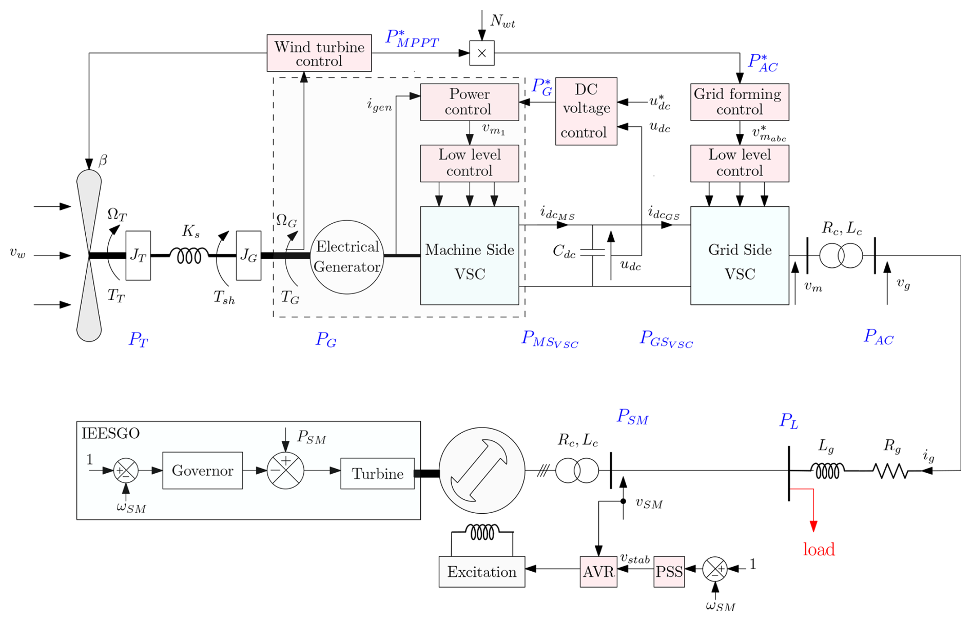
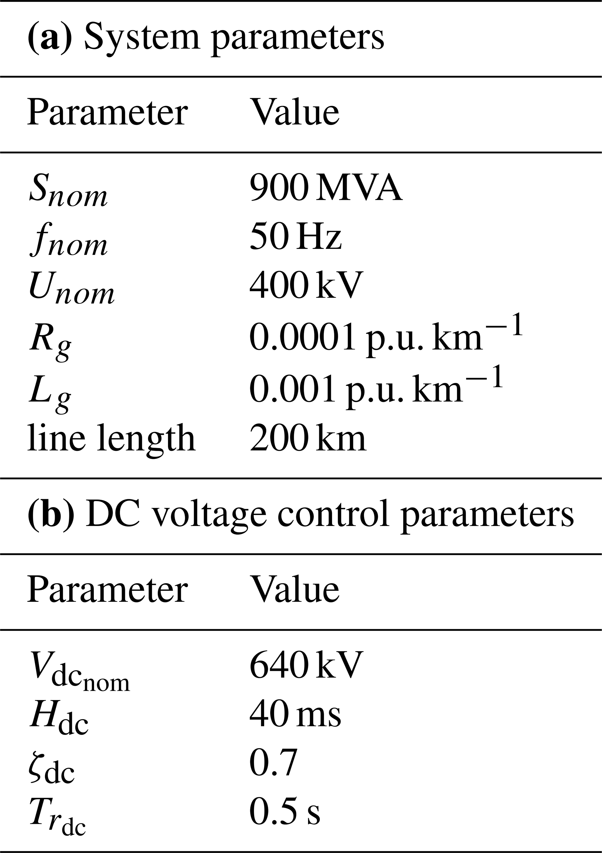
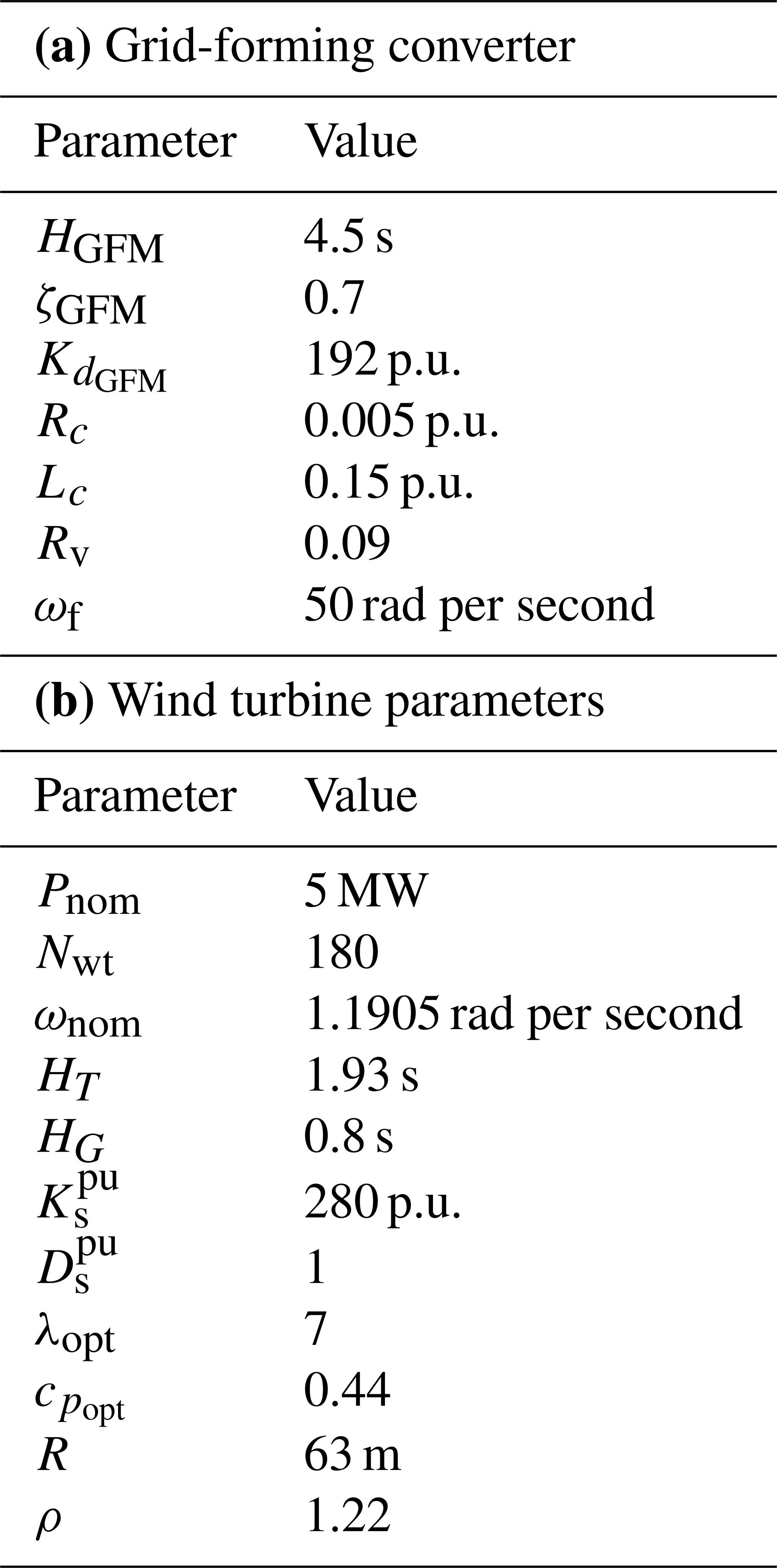
This section introduces the non-linear model of the test case used for electro-magnetic transient (EMT) simulation in MATLAB Simulink to study system dynamics. It consists of a 900 MVA synchronous generator and a 900 MVA aggregated wind farm under grid-forming control, both supplying a load connected through a 200 km transmission line (Shafiu et al., 2006). The wind farm consists of 180 type IV wind turbines of 5 MW, with constant wind speed at each turbine. Figure 1 shows the model including the control loops of both machines. The detailed models of each component are presented in the following sections.

Figure 1 Overall system under study.

2.1 Model of the wind turbine

The wind turbine model comprises several elements that describe either the power part or the control. The detailed presentation of these elements can be found in the next subsections.

2.1.1 Mechanical model

The aerodynamic power is converted to mechanical power P_T given by Eq. (1), where R represents the radius of the wind turbine blades and ρ is the air density.

$$\begin{array}{}\text{(1)}& P_{\mathrm{T}}={\displaystyle \frac{\mathrm{1}}{\mathrm{2}}}\mathit{\rho }\mathit{\pi }{R}^{\mathrm{2}}{c}_{\mathrm{p}}(\mathit{\lambda },\mathit{\beta })v_{\mathrm{w}}^{\mathrm{3}}\end{array}$$

The power coefficient c_p(λ,β) is derived from the tip-speed ratio λ and pitch angle β using Eq. (2) (Avazov, 2022).

$$\begin{array}{}\text{(2)}& c_{\mathrm{p}}=\mathrm{0.73}\left({\displaystyle \frac{\mathrm{151}}{{\mathit{\lambda }}_r}}-\mathrm{0.58}\mathit{\beta }-\mathrm{0.002}{\mathit{\beta }}^{\mathrm{2.14}}-\mathrm{13.2}\right)e^{\frac{-\mathrm{18.4}}{{\mathit{\lambda }}_r}},\end{array}$$

where ${\mathit{\lambda }}_r=\frac{\mathrm{1}}{\mathit{\lambda }-\mathrm{0.1}\mathit{\beta }}-\frac{\mathrm{0.003}}{{\mathit{\beta }}^{\mathrm{3}}+\mathrm{1}}$ and $\mathit{\lambda }=\frac{R{\mathrm{\Omega }}_{\mathrm{T}}}{v_{\mathrm{w}}}$, with Ω_T being the wind turbine rotational speed and v_w being the wind speed. To illustrate, Fig. 3a depicts the variation of the power coefficient as a function of λ with β=0.

Therefore, from P_T it is possible to derive the mechanical torque on wind turbine T_T:

$$\begin{array}{}\text{(3)}& T_{\mathrm{T}}={\displaystyle \frac{P_{\mathrm{T}}}{{\mathrm{\Omega }}_{\mathrm{T}}}}.\end{array}$$

Considering Ω_G as the rotational speed of the generator and T_G as the torque of the generator, Ω_T and Ω_G are derived from the two-mass mechanical model (Eqs. 4–6), where J_T is the turbine inertia constant, J_G is the generator inertia constant, T_sh is the torque on the shaft, K_s is the shaft stiffness, D_s is the damping coefficient, and Δω represents the difference in rotational speed between the turbine Ω_T and the generator Ω_G.

$$\begin{array}{}\text{(4)}& {\displaystyle \frac{\mathrm{d}{\mathrm{\Omega }}_{\mathrm{T}}}{\mathrm{d}t}}={\displaystyle \frac{\mathrm{1}}{J_{\mathrm{T}}}}\left(T_{\mathrm{T}}-T_{\mathrm{sh}}\right)\text{(5)}& {\displaystyle \frac{\mathrm{d}{\mathrm{\Omega }}_{\mathrm{G}}}{\mathrm{d}t}}={\displaystyle \frac{\mathrm{1}}{J_{\mathrm{G}}}}\left(T_{\mathrm{sh}}-T_{\mathrm{G}}\right)\text{(6)}& {\displaystyle \frac{\mathrm{d}{T}_{\mathrm{sh}}}{\mathrm{d}t}}=D_{\mathrm{s}}{\displaystyle \frac{\mathrm{d}\mathrm{\Delta }\mathit{\omega }}{\mathrm{d}t}}+K_{\mathrm{s}}\mathrm{\Delta }\mathit{\omega }\end{array}$$

Figure 2 Two-mass per-unit mechanical model of the wind turbine.

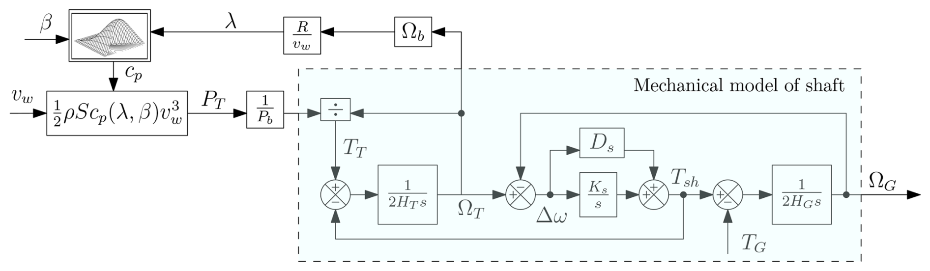
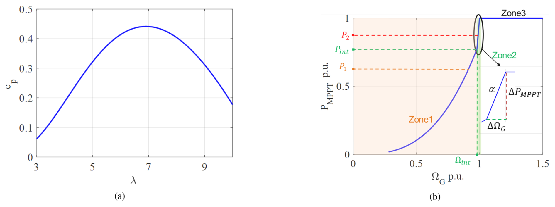
Figure 3 Wind turbine characteristic curves: (a) c_p curve and (b) maximum power point tracking (MPPT) control.

Considering the nominal power P_nom as the base power P_b and the nominal speed Ω_nom as the base speed Ω_b, the per-unit value of the inertia is introduced as $H_{\mathrm{T}}=\frac{\mathrm{0.5}{J}_{\mathrm{T}}{\mathrm{\Omega }}_{\mathrm{b}}^{\mathrm{2}}}{P_{\mathrm{b}}}$ and $H_{\mathrm{G}}=\frac{\mathrm{0.5}{J}_{\mathrm{G}}{\mathrm{\Omega }}_{\mathrm{b}}^{\mathrm{2}}}{P_{\mathrm{b}}}$ for the wind turbine and the generator, respectively. A per-unit coefficient is also introduced for the shaft stiffness $K_{\mathrm{s}}^{\mathrm{pu}}=\frac{K_{\mathrm{s}}{\mathrm{\Omega }}_{\mathrm{b}}^{\mathrm{2}}}{P_{\mathrm{b}}}$ and the damping coefficient $D_{\mathrm{s}}^{\mathrm{pu}}=\frac{D_{\mathrm{s}}{\mathrm{\Omega }}_{\mathrm{b}}^{\mathrm{2}}}{P_{\mathrm{b}}}$. Therefore, Eqs. (5) and (6) can be converted into their per-unit forms:

$$\begin{array}{}\text{(7)}& {\displaystyle \frac{\mathrm{d}{T}_{{\mathrm{sh}}_{\mathrm{pu}}}}{\mathrm{d}t}}=D_{\mathrm{s}}^{\mathrm{pu}}{\displaystyle \frac{\mathrm{d}\mathrm{\Delta }{\mathit{\omega }}_{\mathrm{pu}}}{\mathrm{d}t}}+K_{\mathrm{s}}^{\mathrm{pu}}\mathrm{\Delta }{\mathit{\omega }}_{\mathrm{pu}},\text{(8)}& {\displaystyle \frac{\mathrm{d}{\mathrm{\Omega }}_{{\mathrm{T}}_{\mathrm{pu}}}}{\mathrm{d}t}}={\displaystyle \frac{\mathrm{1}}{\mathrm{2}{H}_{\mathrm{T}}}}\left(T_{{\mathrm{T}}_{\mathrm{pu}}}-T_{{\mathrm{sh}}_{\mathrm{pu}}}\right),\text{(9)}& {\displaystyle \frac{\mathrm{d}{\mathrm{\Omega }}_{{\mathrm{G}}_{\mathrm{pu}}}}{\mathrm{d}t}}={\displaystyle \frac{\mathrm{1}}{\mathrm{2}{H}_{\mathrm{G}}}}\left(T_{{\mathrm{sh}}_{\mathrm{pu}}}-T_{{\mathrm{G}}_{\mathrm{pu}}}\right).\end{array}$$

For simplicity, the subscript “pu” for per unit is disregarded throughout the paper. Hence, Fig. 2 represents the per-unit mechanical model of the wind turbine based on Eqs. (7)–(9).

Additionally, a simplified model can be introduced by neglecting the oscillatory behavior of the turbine. This approach uses a per-unit one-mass mechanical model, where Ω_1mass represents the common rotational speed of both the wind turbine and the generator. Considering their equivalent inertia $H_{\mathrm{1}\mathrm{mass}}=H_{\mathrm{T}}+H_{\mathrm{G}}$, the shaft is then modeled as

$$\begin{array}{}\text{(10)}& {\displaystyle \frac{\mathrm{d}{\mathrm{\Omega }}_{\mathrm{1}\mathrm{mass}}}{\mathrm{d}t}}={\displaystyle \frac{\mathrm{1}}{\mathrm{2}{H}_{\mathrm{1}\mathrm{mass}}}}\left(T_{\mathrm{T}}-T_{\mathrm{G}}\right).\end{array}$$

2.1.2 Wind power conversion strategy and optimization

The power curve of the aggregated wind turbine model is assumed to be the same as the power curve of the individual wind turbine. The power curve of the wind turbine has various operating zones represented in Fig. 3b in per unit (Wu et al., 2016; Krpan and Kuzle, 2018).

In the maximum power point tracking (MPPT) zone referred to as zone 1, it is possible to define an optimal speed for each wind speed v_w to optimize the power generation. This optimal speed is reached by adjusting the generator torque T_G. In this operation mode, the power coefficient and tip-speed ratio have a constant value: c_opt and λ_opt. The maximum power P_zone 1 is given by Eq. (11).

$$\begin{array}{}\text{(11)}& P_{\mathrm{zone}\mathrm{1}}={\displaystyle \frac{\mathrm{1}}{\mathrm{2}{P}_{\mathrm{b}}}}\mathit{\rho }\mathit{\pi }{R}^{\mathrm{2}}{c}_{{\mathrm{p}}_{\mathrm{opt}}}{\left({\displaystyle \frac{{\mathrm{\Omega }}_{\mathrm{G}}{\mathrm{\Omega }}_{\mathrm{b}}R}{{\mathit{\lambda }}_{\mathrm{opt}}}}\right)}^{\mathrm{3}}\end{array}$$

After a given wind speed, the MPPT cannot be applied anymore because the nominal rotation speed is reached. Then, the reference power applied aims to stay around the nominal speed; this operation mode is referred to as speed limitation: zone 2 between two points (P_int, Ω_int) and (1, 1) with slope $\mathit{\alpha }=\frac{\mathrm{1}-P_{\mathrm{int}}}{\mathrm{1}-{\mathrm{\Omega }}_{\mathrm{int}}}$. Then the power P_zone 2 with the slope α is derived as

$$\begin{array}{}\text{(12)}& P_{\mathrm{zone}\mathrm{2}}=\mathit{\alpha }\left({\mathrm{\Omega }}_{\mathrm{G}}-{\mathrm{\Omega }}_{\mathrm{int}}\right)+P_{\mathrm{int}}.\end{array}$$

Finally, when the nominal power is reached, the speed cannot be limited by the reference power anymore; the pitch control is actuated to decrease c_p and limit the power generated by the blades to its nominal value. Hence, this is referred to as power limitation: zone 3 with power P_zone 3,

$$\begin{array}{}\text{(13)}& P_{\mathrm{zone}\mathrm{3}}=\mathrm{1}.\end{array}$$

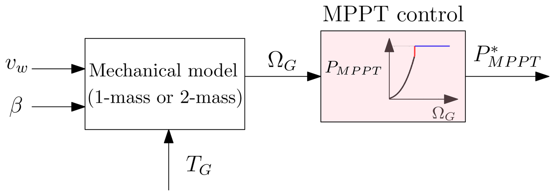
In summary, the operating point of the wind turbine determines the power output $P_{\mathrm{MPPT}}^{*}$ of the MPPT control given by Eqs. (11), (12), or (13) represented in Fig. 4.

Figure 4 Wind turbine MPPT control.

2.1.3 Model of the machine, machine side VSC, and their controls

The generator and machine side voltage source converter (VSC) are considered lossless; therefore, the generator power P_G and power delivered by the machine side VSC $P_{{\mathrm{MS}}_{\mathrm{VSC}}}$ to DC bus are expressed by Eq. (14) with DC bus voltage u_dc and DC current $i_{{\mathrm{dc}}_{\mathrm{MS}}}$ injected into the DC bus.

$$\begin{array}{}\text{(14)}& T_{\mathrm{G}}{\mathrm{\Omega }}_{\mathrm{G}}=P_{\mathrm{G}}=P_{{\mathrm{MS}}_{\mathrm{VSC}}}=u_{\mathrm{dc}}{i}_{{\mathrm{dc}}_{\mathrm{MS}}}\end{array}$$

The electrical power is regulated to a reference value $P_{\mathrm{G}}^{*}$ through a current loop. Due to the fast dynamics of the control, it can be written as

$$\begin{array}{}\text{(15)}& P_{\mathrm{G}}=P_{\mathrm{G}}^{*}.\end{array}$$

Hence, the DC current $i_{{\mathrm{dc}}_{\mathrm{MS}}}$ generated by the machine side VSC is calculated by Eq. (16).

$$\begin{array}{}\text{(16)}& i_{{\mathrm{dc}}_{\mathrm{MS}}}={\displaystyle \frac{P_{\mathrm{G}}^{*}}{u_{\mathrm{dc}}}}\end{array}$$

And equivalent power $P_{{\mathrm{G}}_{\mathrm{eq}}}$ generated by N_wt number of wind turbines is

$$\begin{array}{}\text{(17)}& P_{{\mathrm{G}}_{\mathrm{eq}}}=P_{\mathrm{G}}{N}_{\mathrm{wt}}.\end{array}$$

2.1.4 Grid side VSC model and control

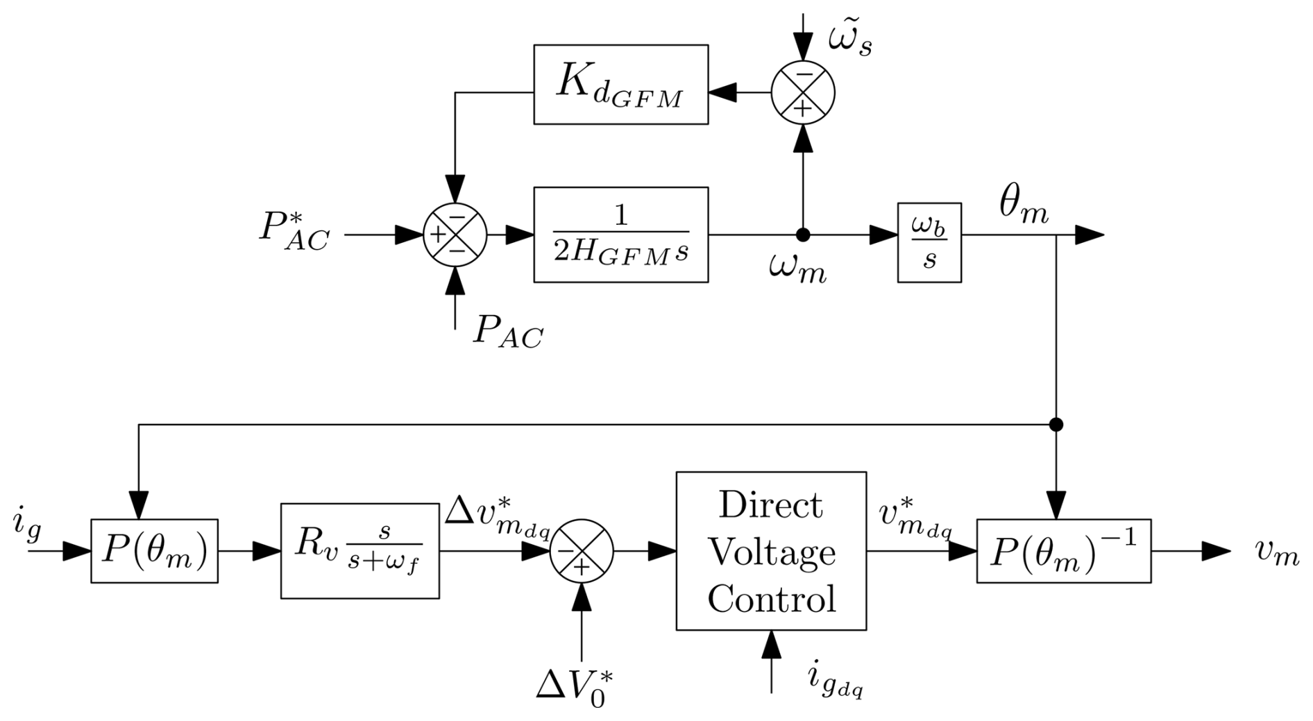
The system is connected to the grid through a VSC. An average model of the VSC is considered, and the control strategy used is grid-forming. The converter modulates the DC bus voltage in order to generate the three-phase voltage v_ma, v_mb, and v_mc. The grid-forming virtual-synchronous-machine (VSM) scheme is shown in Fig. 5 with virtual inertia H_GFM and damping coefficient $K_{{\mathrm{d}}_{\mathrm{GFM}}}={\mathit{\zeta }}_{\mathrm{GFM}}\sqrt{\frac{\mathrm{2}(X_g+X_c)}{{\mathit{\omega }}_b{H}_{\mathrm{GFM}}}}$ designed based on the transmission line impedance X_g, transformer impedance X_c, and damping factor ζ_GFM=0.7 (Rokrok, 2022). VSM controls the active power P_AC to match the reference $P_{\mathrm{AC}}^{*}$ by acting on the modulated voltage reference angle θ_m. The magnitude of the modulated voltage is set to V^*. In order to damp the current oscillations, a transient virtual resistor (TVR) R_v modifies the voltage reference $v_{{\mathrm{m}}_{\mathrm{dq}\mathrm{0}}}^{*}$ (Lamrani et al., 2023). Then the reference modulated $v_{\mathrm{ma}}^{*}$, $v_{\mathrm{mb}}^{*}$, and $v_{\mathrm{mc}}^{*}$ are calculated by the inverse Park transformation P(θ_m)⁻¹. Similar to the machine side converter, the grid side converter is assumed lossless, with $P_{{\mathrm{GS}}_{\mathrm{MSC}}}$ being the power exchanged between DC bus and grid side VSC and given by

$$\begin{array}{}\text{(18)}& P_{{\mathrm{GS}}_{\mathrm{MSC}}}=P_{\mathrm{AC}}.\end{array}$$

Figure 5 Reference model of grid-forming converter.

2.1.5 DC bus model and control

The DC bus is modeled using a simple capacitor C_dc as

$$\begin{array}{}\text{(19)}& C_{\mathrm{dc}}{\displaystyle \frac{\mathrm{d}{u}_{\mathrm{dc}}}{\mathrm{d}t}}=i_{{\mathrm{dc}}_{\mathrm{MS}}}-i_{{\mathrm{dc}}_{\mathrm{GS}}}.\end{array}$$

As for the inertia, it is possible to define an H value, $H_{\mathrm{dc}}=\frac{C_{\mathrm{dc}}{V}_{{\mathrm{dc}}_{\mathrm{b}}}^{\mathrm{2}}}{\mathrm{2}{P}_{\mathrm{b}}}$, where $V_{{\mathrm{dc}}_{\mathrm{b}}}$ is the base DC voltage equal to the nominal voltage of the DC bus. Hence, the DC bus model in per unit with inertia H_dc is expressed as

$$\begin{array}{}\text{(20)}& {\displaystyle \frac{\mathrm{d}{u}_{\mathrm{dc}}^{\mathrm{2}}}{\mathrm{d}t}}={\displaystyle \frac{\mathrm{1}}{H_{\mathrm{dc}}}}\left(P_{\mathrm{G}}-P_{\mathrm{AC}}\right).\end{array}$$

The DC bus control is needed to achieve the stability of the DC bus which depends on the power delivered by the generator side VSC (P_G) and the grid side VSC (P_AC). As demonstrated by Avazov (2022) and Huang et al. (2023), controlling the DC bus voltage through direct action on the generator power is more effective. The control strategy is based on a PI controller.

Hence, the output of the DC bus controller is the reference for the generator $P_{\mathrm{G}}^{*}$, and the reference power of the GFM controller $P_{\mathrm{AC}}^{*}$ for N_wt number of wind turbines is derived from Eqs. (15) and (17) as follows:

$$\begin{array}{}\text{(21)}& P_{\mathrm{AC}}^{*}=P_{{\mathrm{G}}_{\mathrm{eq}}}=P_{\mathrm{MPPT}}^{*}{N}_{\mathrm{wt}}.\end{array}$$

Figure 6 Simplified linearized model of the system.

2.2 Synchronous-machine model

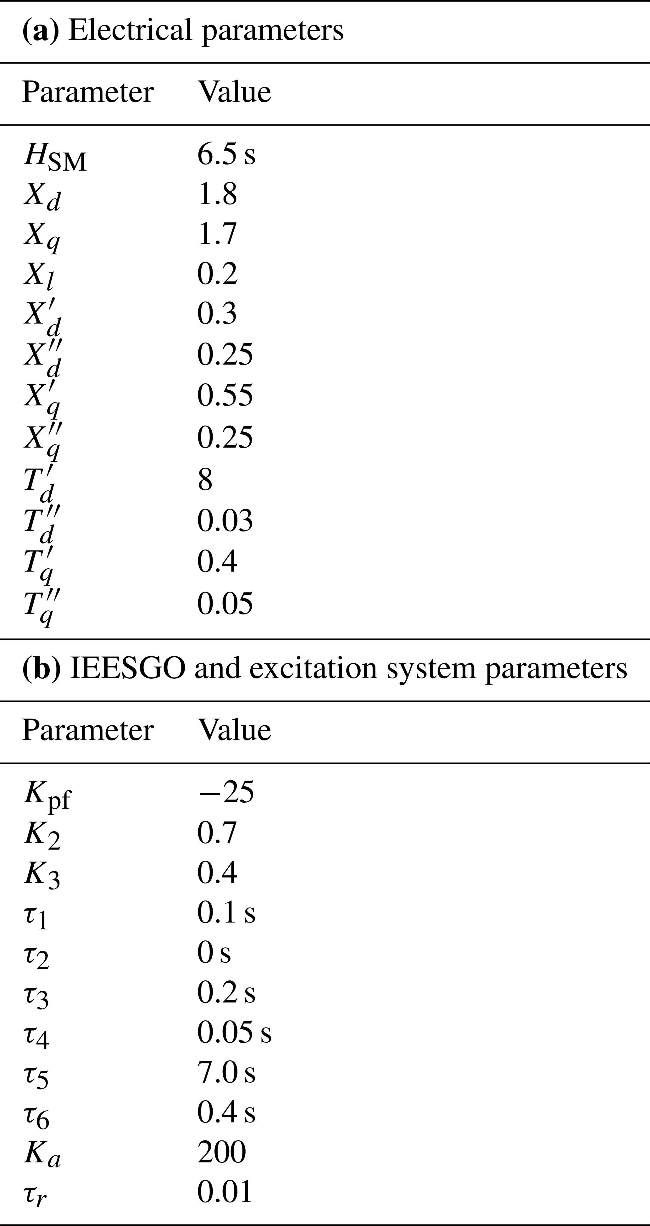
A round rotor type 900 MW synchronous machine is modeled using a detailed eighth-order model with H_SM as the inertia of the synchronous machine and $K_{{\mathrm{d}}_{\mathrm{SM}}}$ as the damping coefficient (P.Kundur, 1994). As illustrated in Fig. 1 it is equipped with the following:

• a transformer with a resistance R_c and a leakage impedance L_c;

• an excitation system of type ST1C (IEEE, 2016) that consist of a main voltage regulator with gain K_a, a low-pass filter with time constant τ_r, and input voltage v_stab from a power system stabilizer;

• a governor modeled as IEESGO (Pourbeik et al., 2013) with power frequency droop gain K_pf and low-pass filters with τ₁ and τ₃ representing the governor dynamics – a three-stage steam turbine is considered with output power P_hp, P_ip, and P_lp and a low-pass filter with τ₄ to include the dynamics of steam valve demonstrated in Fig. 6;

• a power system stabilizer model PSS1A (IEEE, 2016) that consist of two lead–lag filters – one washout filter τ_p5=10 s and one low-pass filter τ_p6=0.01 s – and PSS gain K_PSS=0.

3 Linear models of the system

In order to use the classical tool for dynamic analysis, such as eigenvalues, a linear model is needed. This involves developing a linearized representation of the wind turbine and its control system. Combining this linearized model with that of the synchronous machine results in the linearized system model shown in Fig. 1. By introducing a few additional assumptions, a simplified linearized model can be derived. This simplified model, represented as a block diagram, provides valuable physical insight into the dynamics of the system.

3.1 Reference linear model

The first linear model consists of the following.

1. The linearized model of the wind turbine is obtained by linearizing P_T (Eq. 1) in two components, the $\frac{\mathrm{d}{P}_{\mathrm{T}}}{\mathrm{d}{v}_{\mathrm{w}}}$ positive value for all operating points and the $\frac{\mathrm{d}{P}_{\mathrm{T}}}{\mathrm{d}{\mathrm{\Omega }}_{\mathrm{G}}}$ negative value for all operating points. Even with this simplification, some non-linearities remain in the model. The gain K_MPPT represents the power characteristics to generate $\mathrm{\Delta }{P}_{\mathrm{MPPT}}^{*}$:

   • a.

     in zone 1 by linearizing Eq. (11), $\mathrm{\Delta }{P}_{\mathrm{MPPT}}^{*}=\mathrm{\Delta }{P}_{\mathrm{zone}\mathrm{1}}$ and $K_{\mathrm{MPPT}}=\frac{\mathrm{d}{P}_{\mathrm{zone}\mathrm{1}}}{\mathrm{d}{\mathrm{\Omega }}_{\mathrm{G}}}$;

   • b.

     in zone 2 by linearizing Eq. (12), $\mathrm{\Delta }{P}_{\mathrm{MPPT}}^{*}=\mathrm{\Delta }{P}_{\mathrm{zone}\mathrm{2}}$ and K_MPPT=α;

   • c.

     in zone 3 by linearizing Eq. (13), $\mathrm{\Delta }{P}_{\mathrm{MPPT}}^{*}=\mathrm{\Delta }{P}_{\mathrm{zone}\mathrm{3}}$ and K_MPPT=0.

2. The grid-forming VSC and DC link dynamics model is already linear except for the eight-order model of the synchronous machine which is linearized according to small signal stability analysis (P.Kundur, 1994). The grid is modeled using Kirchhoff's law in the d−q frame for line parameters R_g and L_g and constant impedance load P_L.

Hereafter, for simplicity, the reference linear model is referred to as the linear model.

3.2 Simplified linear model

Using the same linearized model of the wind turbine, the simplified linearized model is developed based on following assumptions.

1. Considering that the energy stored in the capacitor is negligible compared with the energy stored in the inertia, the dynamics of the DC voltage are neglected. Hence, the power P_G is considered equal to P_AC using Eq. (15), and it can be written as

   $$\begin{array}{}\text{(22)}& P_{\mathrm{AC}}=P_{\mathrm{G}}^{*}.\end{array}$$

2. All of the AC system is considered in phasor representation with active power flow between voltage source P_AC and synchronous machine P_SM that depends on angle δ_m and δ_SM, corresponding to the voltage at grid-forming converter v_m and synchronous machine v_SM, respectively. The quasi-static representation of the grid, as described by Santos Pereira (2020), with load P_L and assuming that voltage angles are small, is as follows:

   $$\begin{array}{}\text{(23)}& {\displaystyle }& {\displaystyle }\mathrm{\Delta }{P}_{\mathrm{AC}}={\displaystyle \frac{\mathrm{\Delta }{\mathit{\delta }}_m-\mathrm{\Delta }{\mathit{\delta }}_{\mathrm{SM}}}{X_{\mathrm{AC}}+X_{\mathrm{SM}}}}-{\displaystyle \frac{X_{\mathrm{SM}}\mathrm{\Delta }{P}_{\mathrm{L}}}{X_{\mathrm{AC}}+X_{\mathrm{SM}}}},\text{(24)}& {\displaystyle }& {\displaystyle }\mathrm{\Delta }{P}_{\mathrm{AC}}={\displaystyle \frac{\mathrm{\Delta }{\mathit{\delta }}_{\mathrm{SM}}-\mathrm{\Delta }{\mathit{\delta }}_m}{X_{\mathrm{AC}}+X_{\mathrm{SM}}}}+{\displaystyle \frac{X_{\mathrm{AC}}\mathrm{\Delta }{P}_{\mathrm{L}}}{X_{\mathrm{AC}}+X_{\mathrm{SM}}}},\end{array}$$

   with $X_{\mathrm{AC}}=X_c+X_g$ and X_SM=X_c, neglecting the resistance. These equations are used to obtain the network matrix K_network as

   $$\begin{array}{}\text{(25)}& \begin{array}{rl}\left[\begin{array}{c}\mathrm{\Delta }{P}_{\mathrm{AC}}\\ \mathrm{\Delta }{P}_{\mathrm{SM}}\end{array}\right]=& \underset{K_{\mathrm{network}}}{\underbrace{{\displaystyle \frac{\mathrm{1}}{X_{\mathrm{AC}}+X_{\mathrm{SM}}}}\left[\begin{array}{ccc}\mathrm{1}& -\mathrm{1}& -X_{\mathrm{SM}}\\ -\mathrm{1}& \mathrm{1}& X_{\mathrm{AC}}\end{array}\right]}}\\ & \left[\begin{array}{c}\mathrm{\Delta }{\mathit{\delta }}_m\\ \mathrm{\Delta }{\mathit{\delta }}_{\mathrm{SM}}\\ \mathrm{\Delta }{P}_L\end{array}\right].\end{array}\end{array}$$

3. For the simplified model of a synchronous machine and governor, a second-order equivalent mechanical model is considered. All other internal dynamics are neglected. The damping coefficient $K_{{\mathrm{d}}_{\mathrm{SM}}}$ represents the combined damping effects in the system, which mainly include the effect of the synchronous machine's damper windings, which is neglected in this simplified model. Due to the non-linearity of the synchronous machine, its value is sensitive to the operating point.

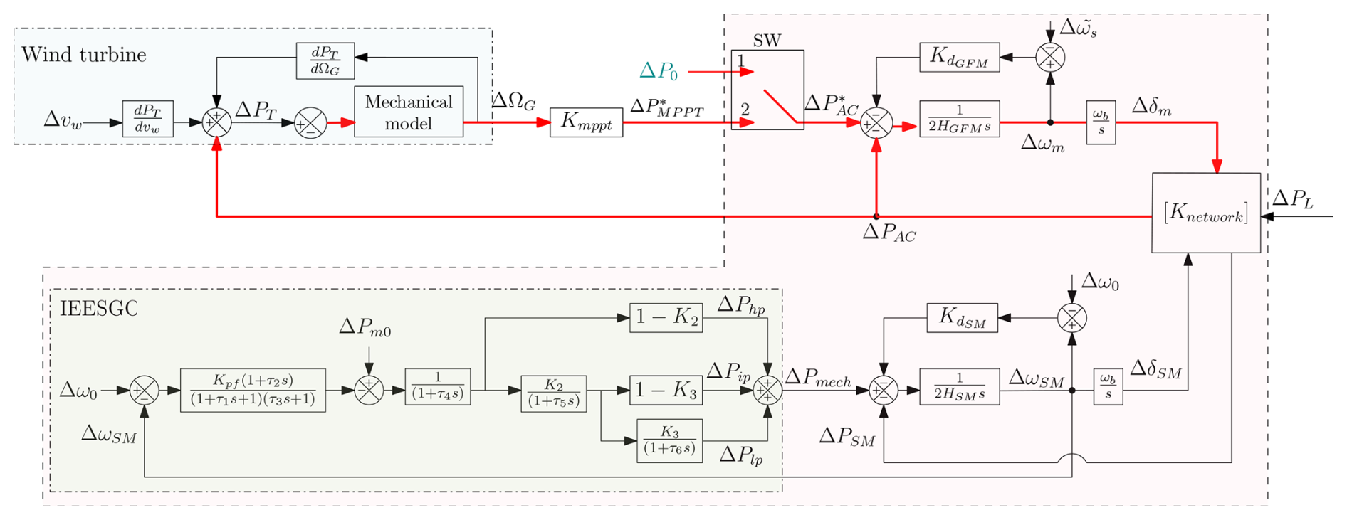
The simplified linearized model of the system is illustrated in Fig. 6. This model is only used to explain the different couplings in the system. One of these couplings is inter-area oscillations (in rose area), which primarily occur in large power systems. The other is the effect of using GFM control on the internal behavior of a single wind turbine. Both phenomena are relevant to the study, but they do not address the same level of power. To merge both models into a single overall model, a strong assumption is made that a full wind farm model is equivalent to a wind turbine model multiplied by the number of wind turbines given in Eq. (17).

The dynamics of linear and simplified linear models are compared with the non-linear model for two operating points, OP₁=0.67 p.u. and OP₂=0.87 p.u., corresponding to the MPPT zone 1 and speed limitation zone 2 shown in Fig. 3b. Since the operating point of the synchronous machine is modified, the $K_{{\mathrm{d}}_{\mathrm{SM}}}$ value has to be adjusted: 30 p.u. for operating point OP₁ and 10 p.u. for operating point OP₂. These values are obtained by the trial and error method by comparing the dynamics with the non-linear model of the synchronous machine. The mechanical model of the wind turbine used is the one-mass model based on Eq. (10). A load step of ΔP_L=0.03 p.u. is applied at 10 s. The resulting variations in system dynamics are shown in Figs. 7 and 8 for operating points OP₁ and OP₂, respectively.

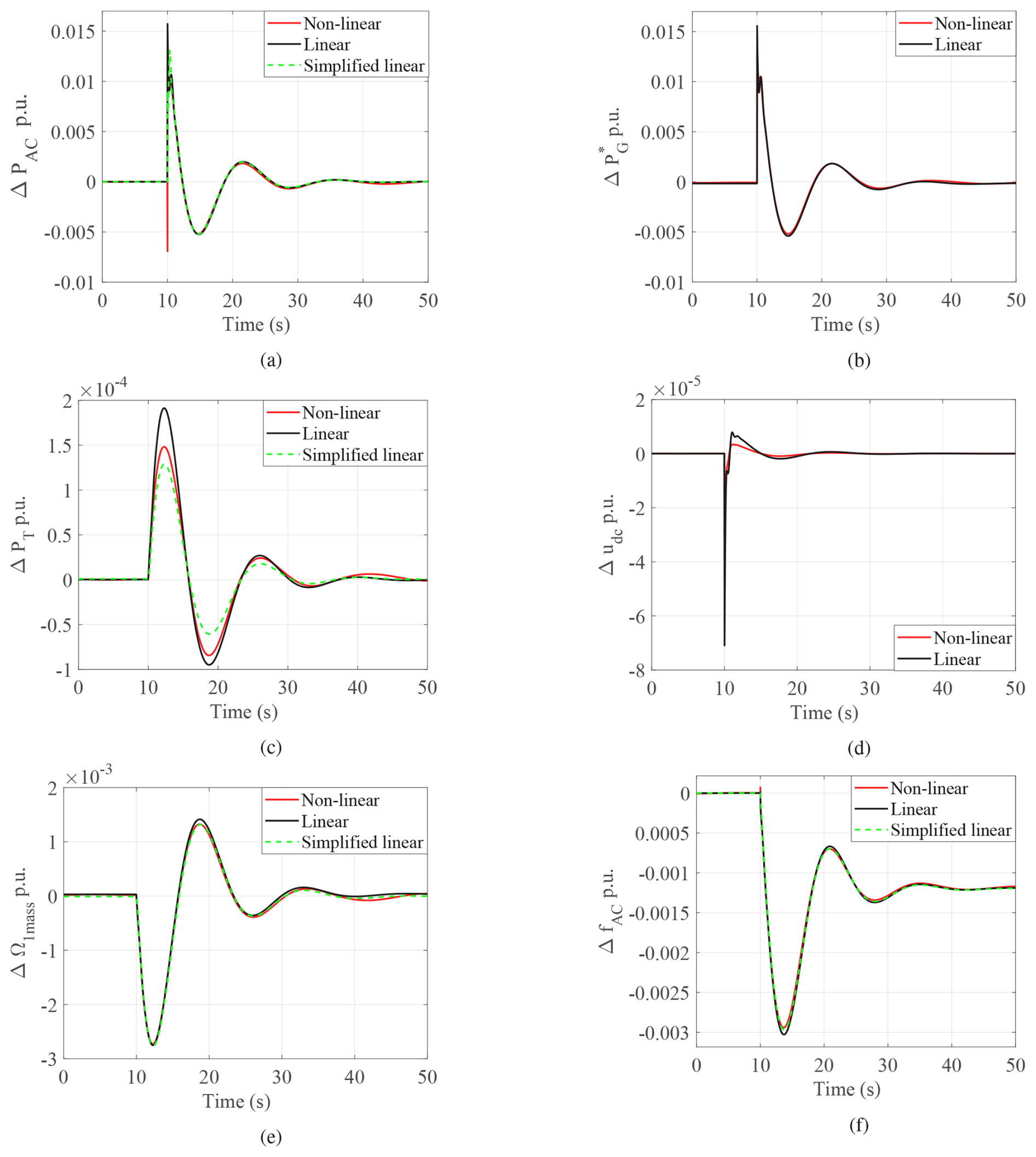
Figure 7 Validation of linear models in zone 1: (a) AC side power P_AC, (b) reference DC power $P_{\mathrm{G}}^{*}$, (c) wind turbine power P_T, (d) DC voltage u_dc, (e) wind turbine speed Ω_1mass, and (f) AC side frequency f_AC.

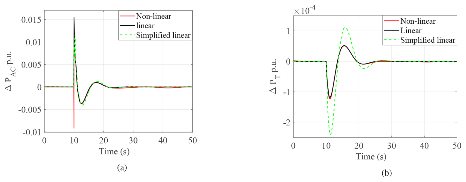
Figure 8 Validation of linear models in zone 2: (a) AC side power P_AC and (b) wind turbine power P_T.

Due to the assumption in Eq. (22) used for the simplified linear model, the variation in reference power Fig. 7b and DC bus voltage Fig. 7d are shown using only the linear model. Figure 7b and e show that after the load step, the imbalance between power delivered by GFM and that generated by the wind turbine slows down the turbine. From Fig. 7a and b, it is observed that the dynamics of the active power align with its reference, thereby confirming the validity of Eq. (22, whereas Fig. 7d illustrates the small variation in DC bus voltage, which is also true for operating point OP₂. Thus, only the variation in AC side power and wind turbine power is demonstrated in Fig. 8 for OP₂. Comparing wind turbine dynamics for two operating points, Figs. 7c and 8b reveal a slight variation in ΔP_T in both linearized models. The first difference comes from the linearization applied to the non-linear model to obtain the linearized model. Then, a second level of simplification is proposed to obtain the so-called “simplified linear” model: the DC link is neglected, and a simple second-order approximation of the synchronous machine is used. The aim of this simplified model is to be sufficiently simple to highlight the main electromechanical couplings in this complex system, even if some accuracy is lost due to the assumptions made. Further, comparing Figs. 7a and 8a, it is observed that the inertial response provided by the GFM converter is more for operating point OP₁.

Table 1 Comparative analysis of eigenvalues for different systems.

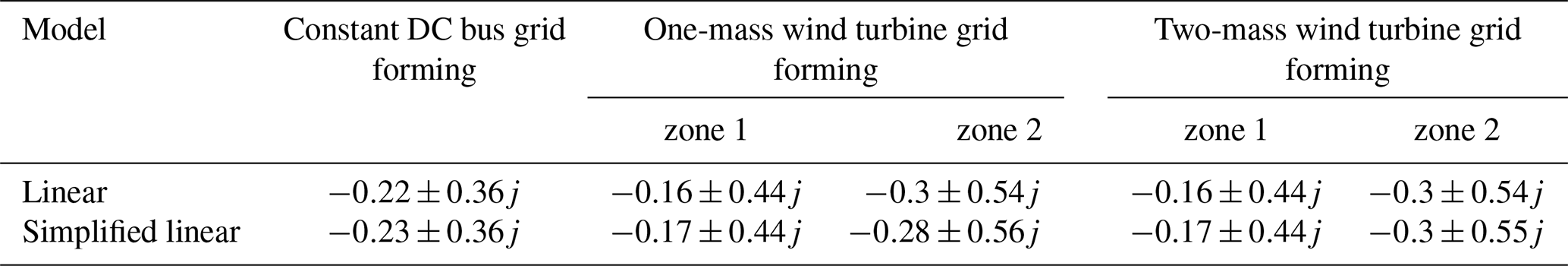
Table 1 shows the dominant mode for different wind turbine models. It shows that the simplified model reproduces the dominant frequency modes even though $K_{{\mathrm{d}}_{\mathrm{SM}}}$ is different. Therefore, the linear models are validated, and the following sections provide further insight into the effects of variation in the operating zone.

4 Analysis of the influence of the wind turbine on the system dynamics and improvements

4.1 Highlighting the main couplings in the system

The simplified linearized model shown in Fig. 6 is considered to explain different couplings in the system. In the case of a constant DC bus for the grid side VSC (switch SW in position 1 with constant active power reference ΔP₀), this figure reveals a well-known inter-area oscillation scheme similar to what can be found with two synchronous machines connected via a transmission grid (rose area in Fig. 6). The main difference is that H_GFM and D_GFM are controlled variables that can be chosen by the control. Hence, the characteristics of the inter-area oscillation modes in terms of frequency and damping can be strongly modified by the choice of these parameters (Baruwa and Fazeli, 2021; Xue et al., 2024).

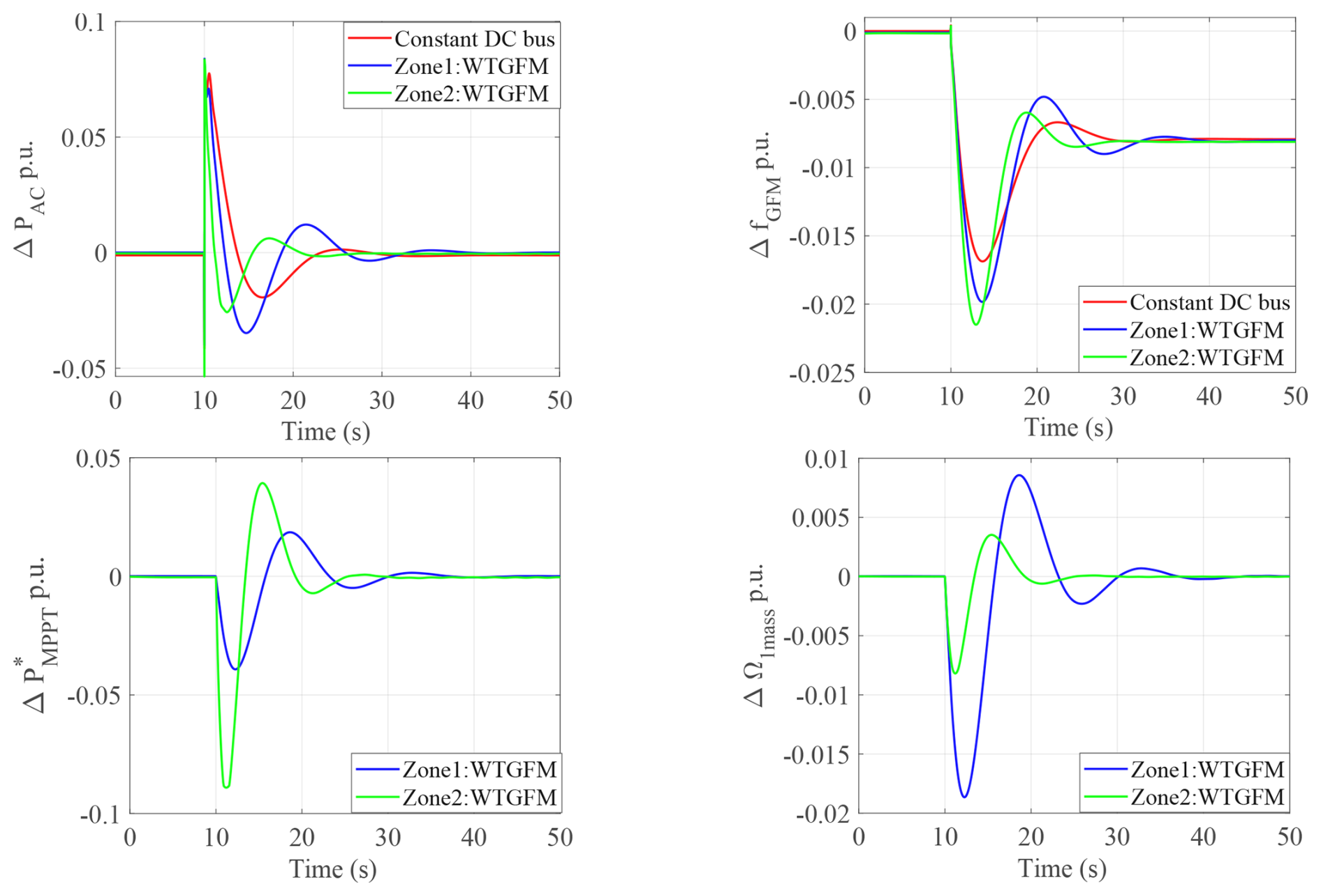
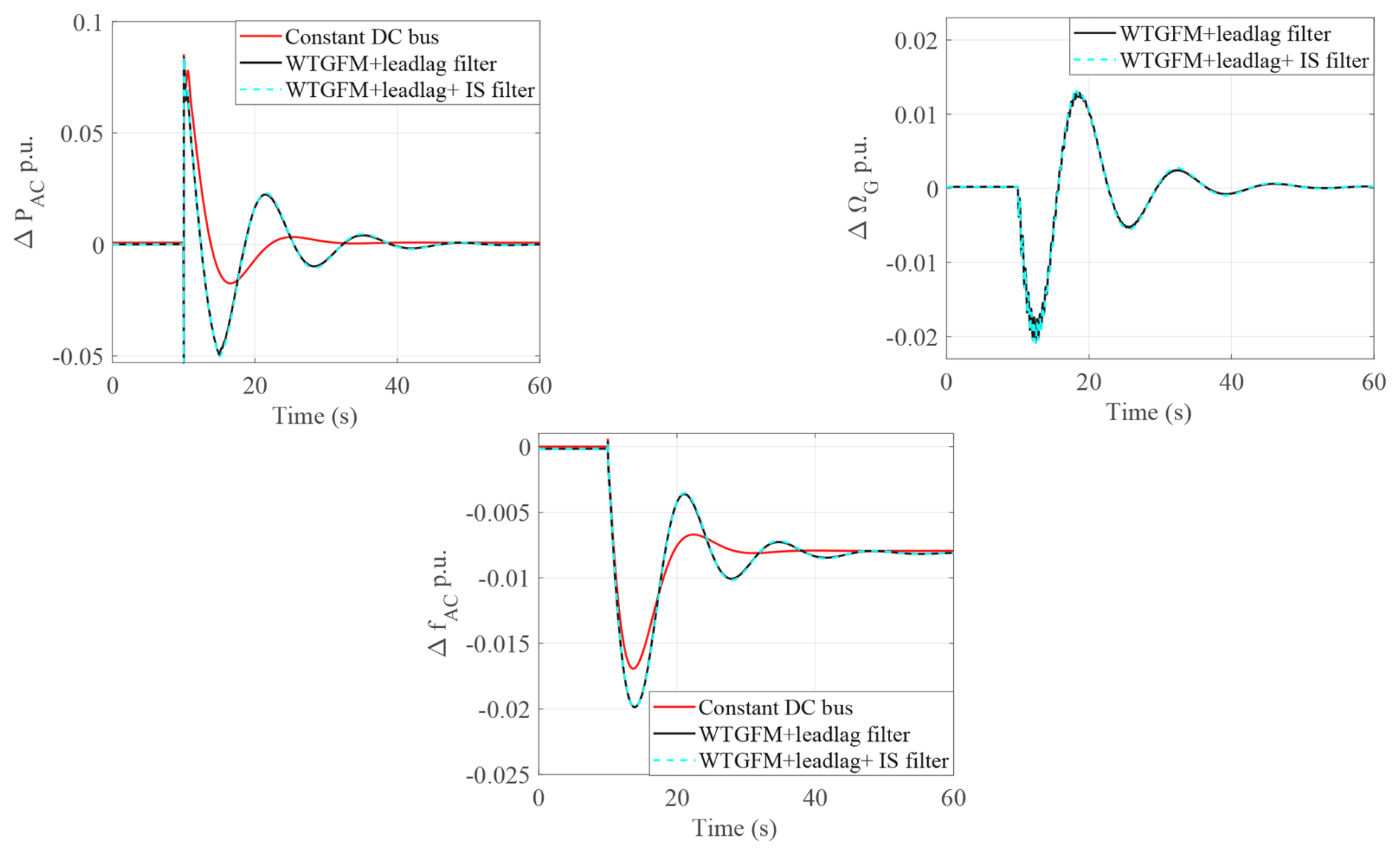
Figure 9 Inertial effect and frequency response of the system with a one-mass wind turbine for a load step of 0.2 p.u. at 10 s.

When SW is in position 2, the simplified linearized model shows that the wind turbine dynamics modify these oscillation modes. Indeed, an additional loop (in red in the system) is added to the system. This loop interacts with the previous modes and modifies the poles and damping as shown in Table 1.

With physical insight from Fig. 6 and EMT simulation Fig. 9, it can be understood that the wind turbine control tends to counteract the inertial effect brought to the grid by the GFM converter. The control decreases the $P_{\mathrm{MPPT}}^{*}$ signal to recover the optimal rotational speed Ω_G. The effect of this additional loop is to decrease the energy that is exchanged with the grid and to decrease the inertial effect. A possible solution to recover the expected inertial effect will be presented in the next section. Due to the non-linearity of the loop, the system dynamics vary depending on the operating point. The gain K_MPPT increases significantly from zone 1 to zone 2, leading to increased system dynamics, as shown in Table 1.

It is also interesting to compare the dynamics of the system by using a one-mass or two-mass model for the drivetrain. The two-mass model offers a more comprehensive understanding of turbine dynamics, particularly in the low-frequency range. In Fig. 10c, a clear decoupling is observed between these eigenvalues and the oscillation modes of the wind turbine itself as the overall grid side dynamics remain unaffected when employing either a one-mass model or a two-mass model in zone 1. However, in zone 2, where faster dynamics dominate as the equivalent gain K_MPPT is higher, the introduction of the two-mass model induces oscillatory behavior shown in Fig. 10.

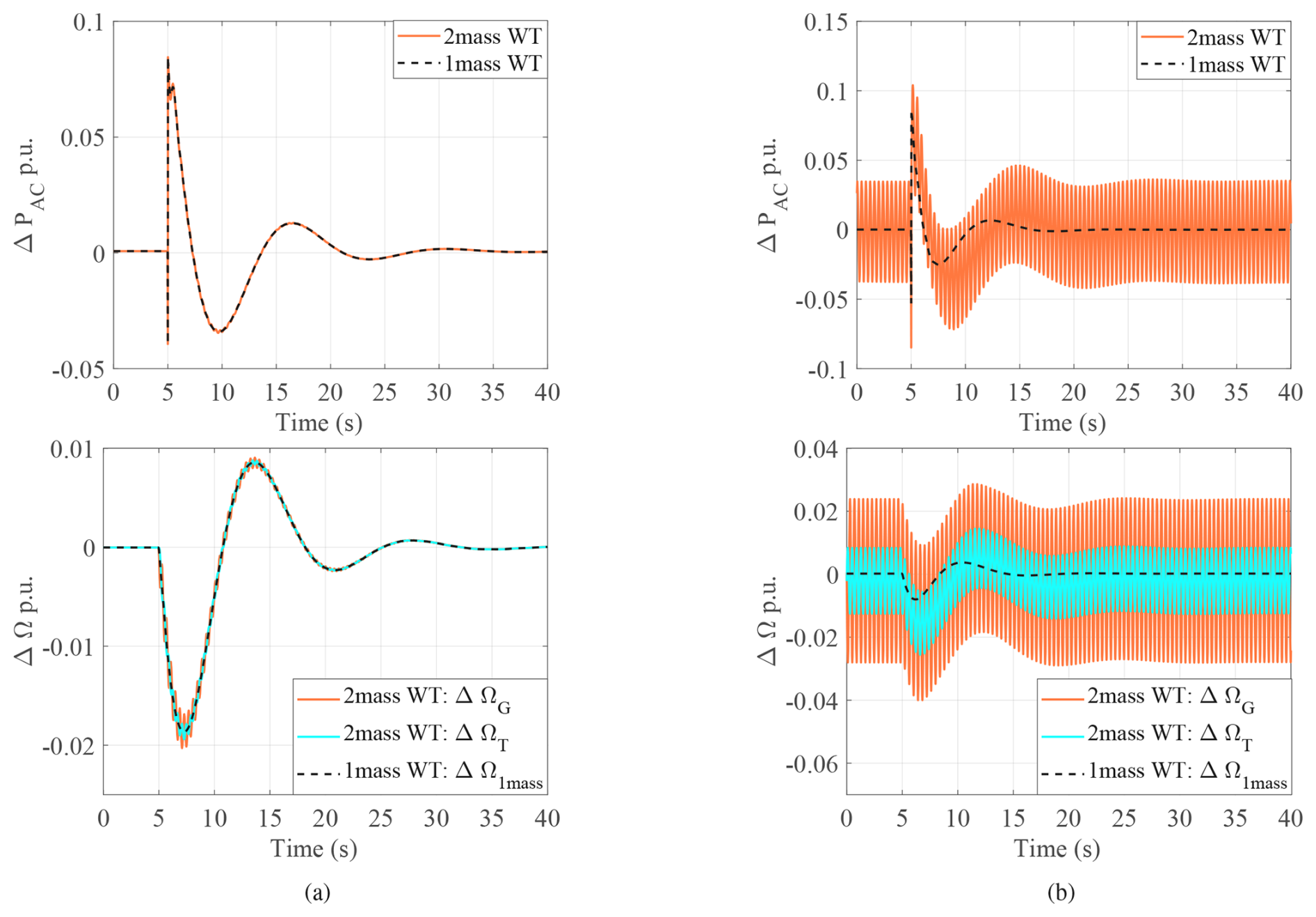
Figure 10 Analysis of different mechanical systems of a wind turbine under a 0.2 p.u. load step for (a) zone 1 (OP1) and (b) zone 2 (OP2).

This section highlighted a new type of coupling due to the connection of a wind turbine to a GFM converter. The resulting undesirable phenomena identified can be mitigated by incorporating dedicated filters into the control loop. Two possible solutions are presented in the following sections.

4.2 Damping the mechanical oscillations using input-shaping filter

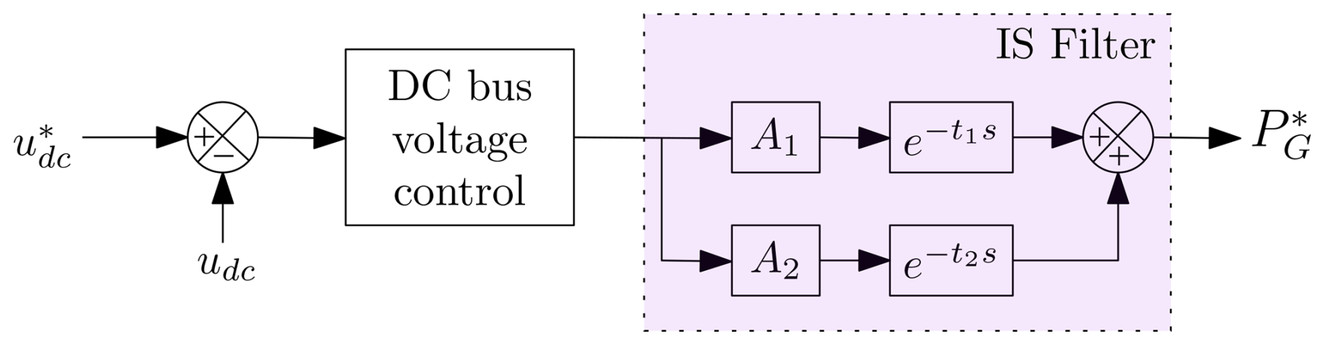
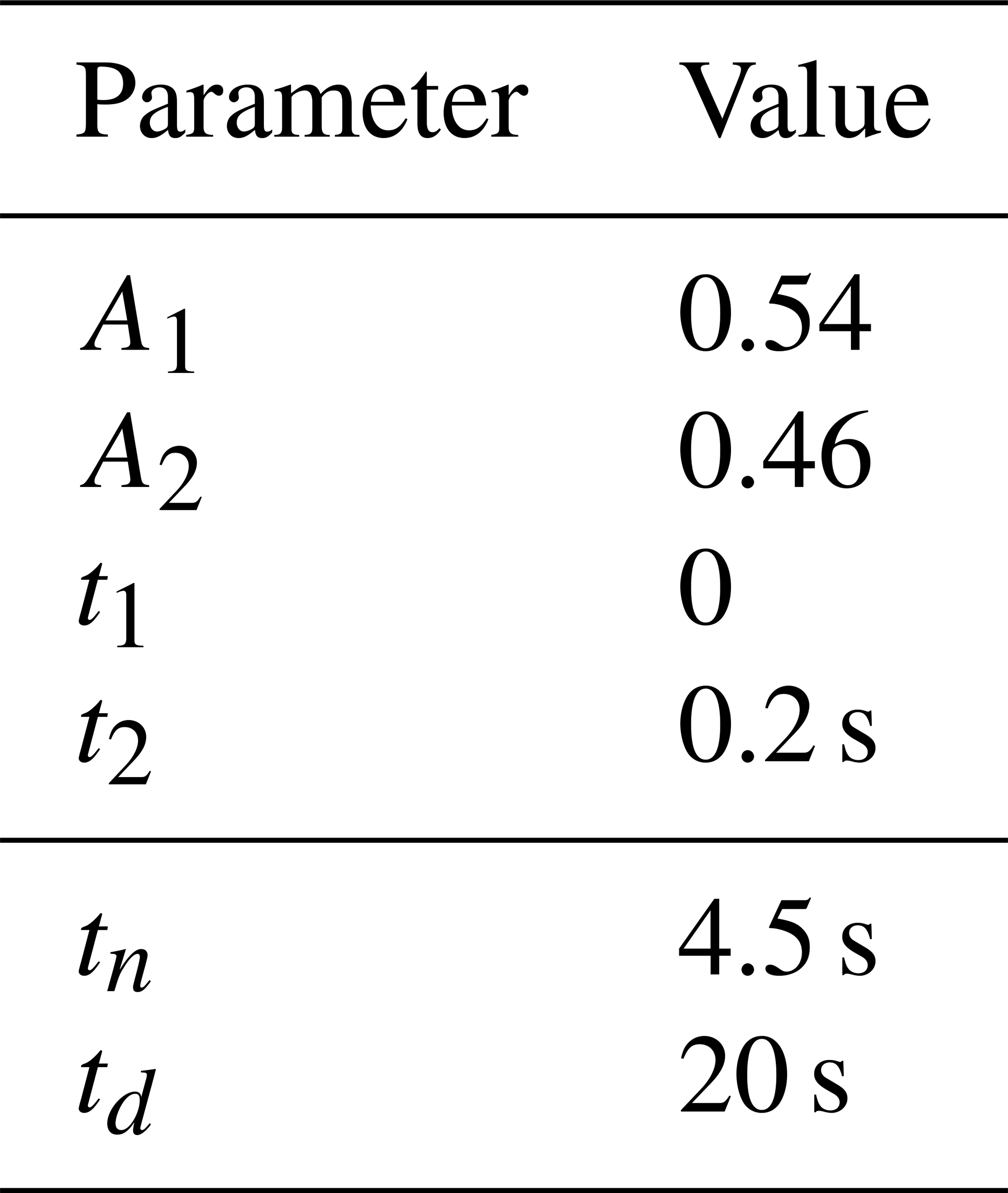
In Avazov (2022), an input-shaping filter was proposed for inclusion in the DC bus voltage control loop. The principle of input shaping is to modify a controlled reference signal by a convolution with a sequence of impulses to get a system response without oscillations. One type of these filters is known as a zero-vibration (ZV) filter, allowing us to achieve the zero level of residual vibrations (Huey et al., 2008). The design of the filter depends on the number of pulses, their amplitude (A_k), and the time of occurrence (t_k). A two-pulse ZV filter as shown in Fig. 11 can be expressed with amplitude A₁, A₂ and time t₁, t₂ in Laplace domain:

$$\begin{array}{}\text{(26)}& \mathrm{IS}\left(s\right)=A_{\mathrm{1}\mathrm{f}}{e}^{-t_{\mathrm{1}}s}+A_{\mathrm{2}\mathrm{f}}{e}^{-t_{\mathrm{2}}s},\end{array}$$

with the necessary requirements as $\mathrm{0}⩽t_{\mathrm{1}}<t_{\mathrm{2}}$ and $A_{\mathrm{1}\mathrm{f}}+A_{\mathrm{2}\mathrm{f}}=\mathrm{1}$.

Figure 11 DC bus voltage control and input-shaping (IS) filter as presented in Avazov (2022).

The resulting finite impulse response filter formed can reduce vibrations in the mechanical system, with the drivetrain oscillatory frequency ω_damp corresponding to drivetrain oscillatory mode $s=\mathit{\sigma }+j{\mathit{\omega }}_{\mathrm{damp}}$ as follows:

$$\begin{array}{}\text{(27)}& t_{\mathrm{1}}=\mathrm{0}{t}_{\mathrm{2}}=t_{\mathrm{1}}+{\displaystyle \frac{\mathit{\pi }}{{\mathit{\omega }}_{\mathrm{damp}}}}.\end{array}$$

Thus, the pulse amplitudes are determined from drivetrain mode are

$$\begin{array}{}\text{(28)}& A_{\mathrm{1}}={\displaystyle \frac{e^{\frac{\mathit{\zeta }\mathit{\pi }}{\sqrt{\mathrm{1}-{\mathit{\zeta }}^{\mathrm{2}}}}}}{\mathrm{1}+e^{\frac{\mathit{\zeta }\mathit{\pi }}{\sqrt{\mathrm{1}-{\mathit{\zeta }}^{\mathrm{2}}}}}}}{A}_{\mathrm{2}}=\mathrm{1}-A_{\mathrm{1}}.\end{array}$$

Figure 12 Proposed solution: integration of the IS filter in the system.

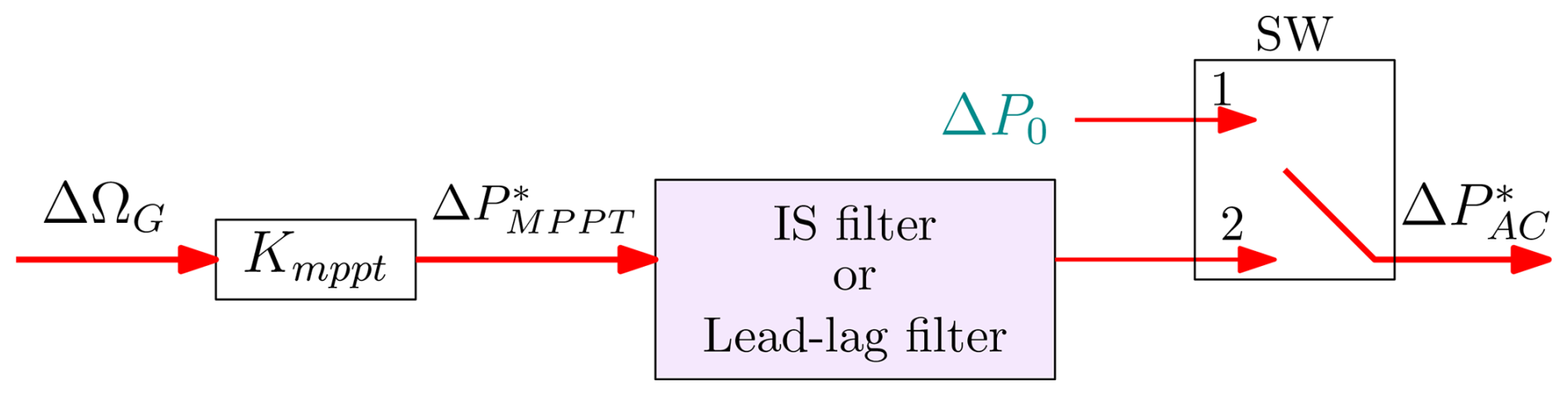
The drivetrain oscillation frequency of the mechanical system of the wind turbine identified from Fig. 10 is 15.7 rad per second. Hence, the ZV filter is designed for ω_damp=15.7 rad per second using Eqs. (27)–(28); parameters are summarized in Table A4. The limitation of this method is to introduce quite a large delay in the control since t₂ is quite large and depends on a low-frequency mechanical mode. As it has been shown that the energy stored in the capacitor is negligible, and the power P_G is nearly equal to P_AC, another solution is then to place this input-shaping filter to generate the reference of the active power shown in Fig. 12.

The designed IS filter is tested for variable input wind speed v_w within zone 1 and zone 2 and a load step of 0.2 p.u. at 30 s as shown in Fig. 13. The analysis indicates that drivetrain oscillations, which result from a high gain of K_MPPT, are effectively damped by the IS filter.

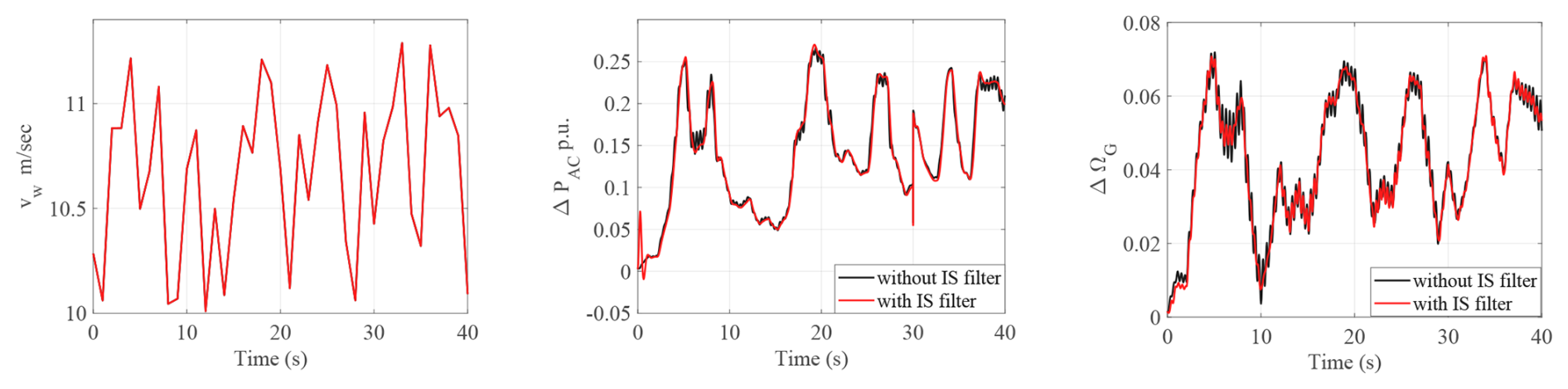
Figure 13 Testing of the input-shaping (IS) filter for variable wind speed v_w and a 0.2 p.u. step load at 30 s.

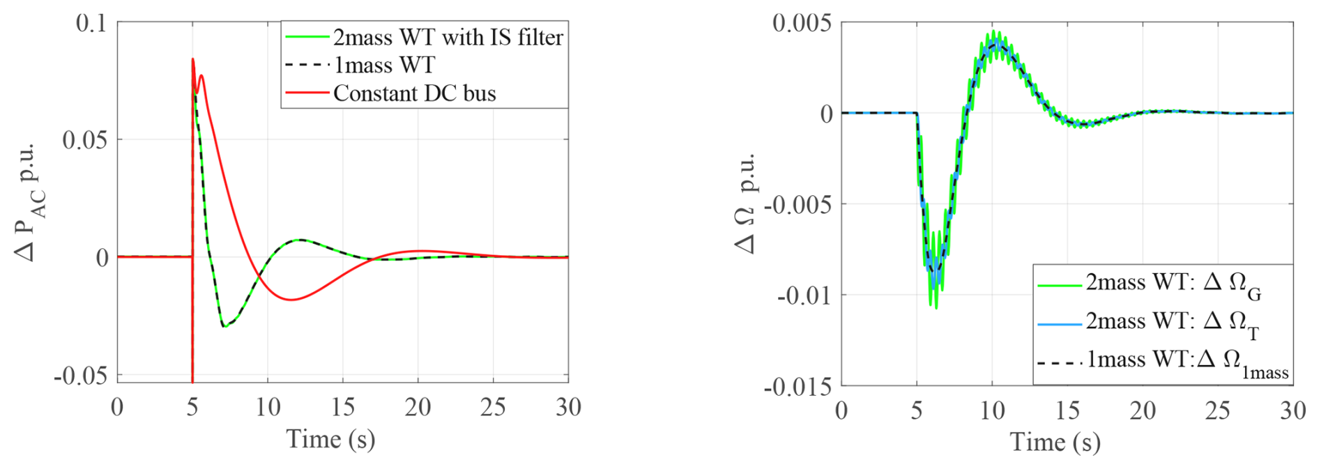
Furthermore, the comparative analysis of the two-mass model of a wind turbine with an IS filter with the one-mass model is presented in Fig. 14. This analysis shows that the inertial response of the two-mass model and the input-shaping (IS) control is similar to a one-mass model. And comparing the wind turbine speed with Fig. 10 proves the effectiveness of the IS filter.

Figure 14 Effect of the input-shaping filter in zone 2.

4.3 Use of a lead–lag filter to increase the inertial effect

As described before, the inertial response of a GFM-controlled wind turbine is different from a GFM-controlled VSC with a constant DC bus. To enhance the inertial response of the GFM wind turbine, the MPPT control operation can be deliberately delayed through the implementation of a low-pass filter. This approach serves to smooth the power reference signal, effectively decoupling the GFM inertial effect from the mechanical dynamics of the wind turbine. By introducing this delay, the system mitigates rapid fluctuations in power demand that could otherwise interfere with the turbine's mechanical stability. Additionally, this strategy ensures a more predictable inertial contribution, thereby improving the overall behavior of the wind turbine in response to grid disturbances. This additional low-pass filter is expressed in Eq. (29).

$$\begin{array}{}\text{(29)}& {\displaystyle \frac{P_{\mathrm{MPPT}}^{*}}{P_{\mathrm{MPPT}}}}={\displaystyle \frac{\mathrm{1}}{\mathrm{1}+t_{d}s}}\end{array}$$

To correctly tune this filter, the system response has been tested for various lag coefficients (t_d) at OP₁ for the 0.2 p.u. load step at 10 s.

The analysis in Fig. 15a shows that using a t_d=20 s low-pass first-order filter provides an improved inertial effect, and the frequency response of the AC tends to be the same as with a constant DC bus voltage. It may be possible to increase the filter time constant to 30 s, but this would result in slower mechanical modes. In any case, the mechanical counterpart is a larger speed variation of the wind turbine, which can be explained by the fact that the wind turbine provides more inertial effect to the grid. As it can be shown in Fig. 15a, adding a filter tends to decrease the damping of the dominant mode. A possible solution is to add a lead effect (Eq. 30) to improve the transient response.

$$\begin{array}{}\text{(30)}& {\displaystyle \frac{P_{\mathrm{MPPT}}^{*}}{P_{\mathrm{MPPT}}}}={\displaystyle \frac{\mathrm{1}+t_{n}s}{\mathrm{1}+t_{d}s}}\end{array}$$

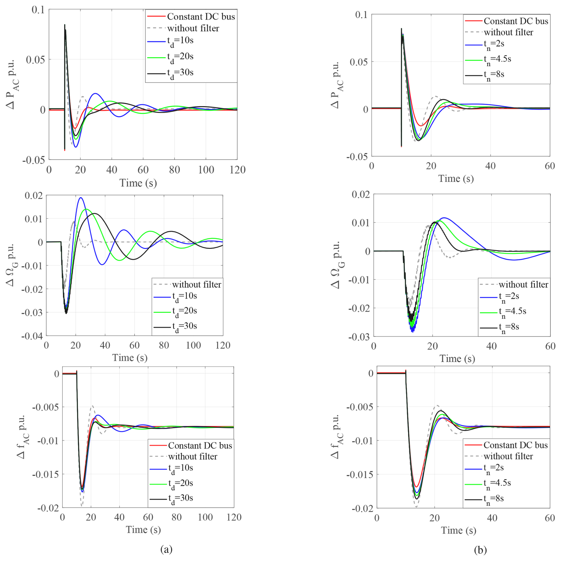
Figure 15 Inertia enhancement for OP₁ in zone 1: (a) with a low-pass filter and (b) with a lead–lag filter.

The system is tested for various lead coefficients (t_n) in zone 1 while keeping the delay t_d=20 s. The choice is a trade-off between the improvement of the damping of the mode and the decrease of the inertial effect. The resulting Fig. 15b shows that t_n=4.5 s is a better choice. When the tuning is achieved in zone 1, the effectiveness of the lead–lag filter in zone 2 has to be checked. As previously mentioned, the large increase of the gain K_MPPT leads to a more oscillating behavior, as seen in Fig. 16, with no possibility of improving this damping. In this figure, it can be observed that the drive train oscillations are well damped by the filter, eliminating the need to add the input-shaping filter in series with the lead–lag filter.

Figure 16 Inertial response in zone 2 with a lead–lag filter.

4.3.1 Robustness assessment under varying system conditions

This section gives an analysis of the performance of the proposed solution for different loading and system conditions. It is presented for both of the operating points OP₁ and OP₂ corresponding to zone 1 and zone 2 operation of the wind turbine.

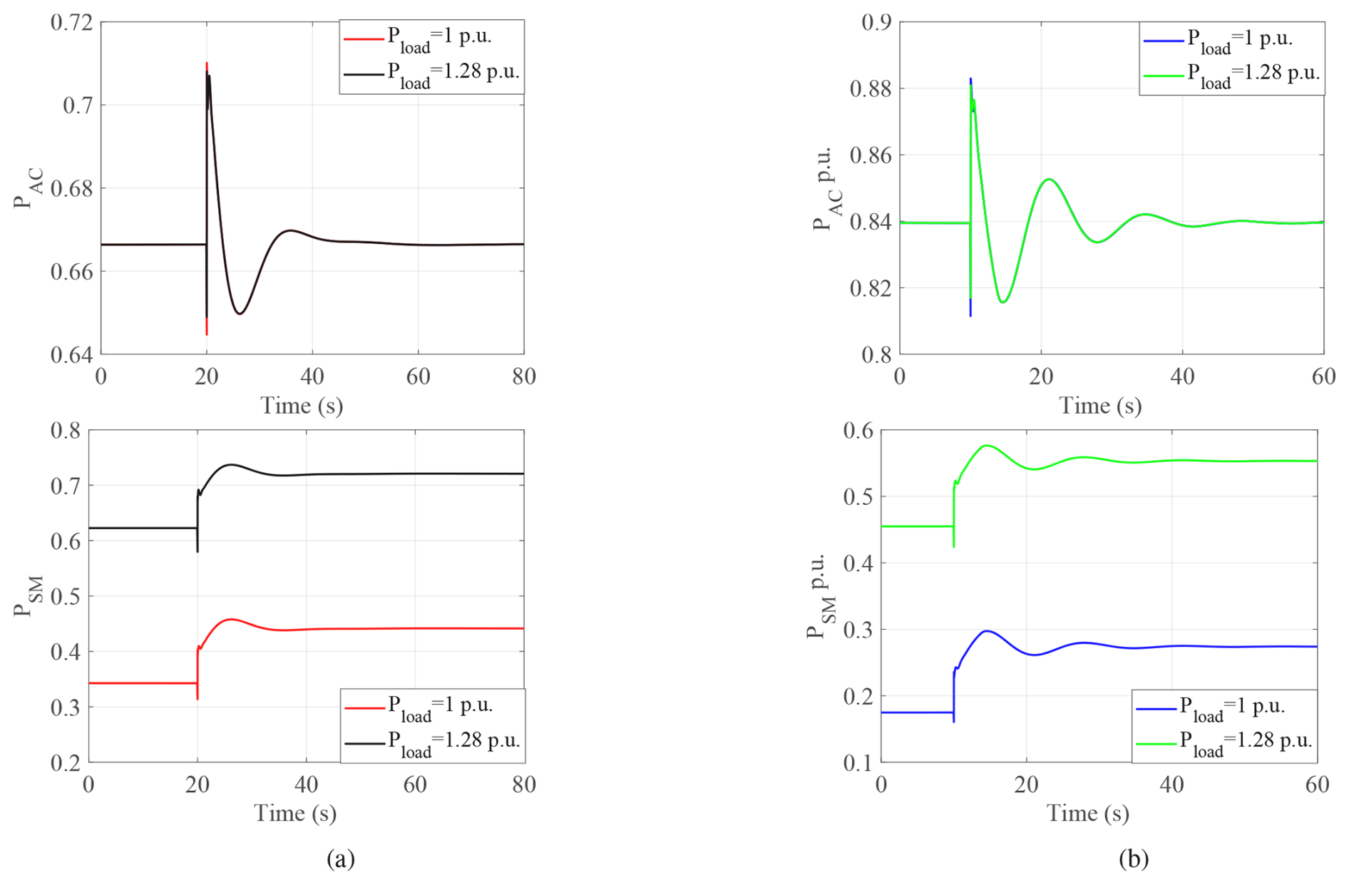
Figure 17 System response to a 0.1 p.u. load step at 10 s for operating points (a) OP₁ and (b) OP₂.

For different loading conditions, the load connected near the synchronous machine is increased from 1 to 1.28 p.u. Figure 17 shows that the load increase is provided by a synchronous machine, which serves as the swing bus of the system. Additionally, by comparing P_AC it can be seen that the dynamic behavior is less damped for the OP₂. The simplified model can help to understand this phenomenon since the gain K_MPPT increases significantly from zone 1 to zone 2.

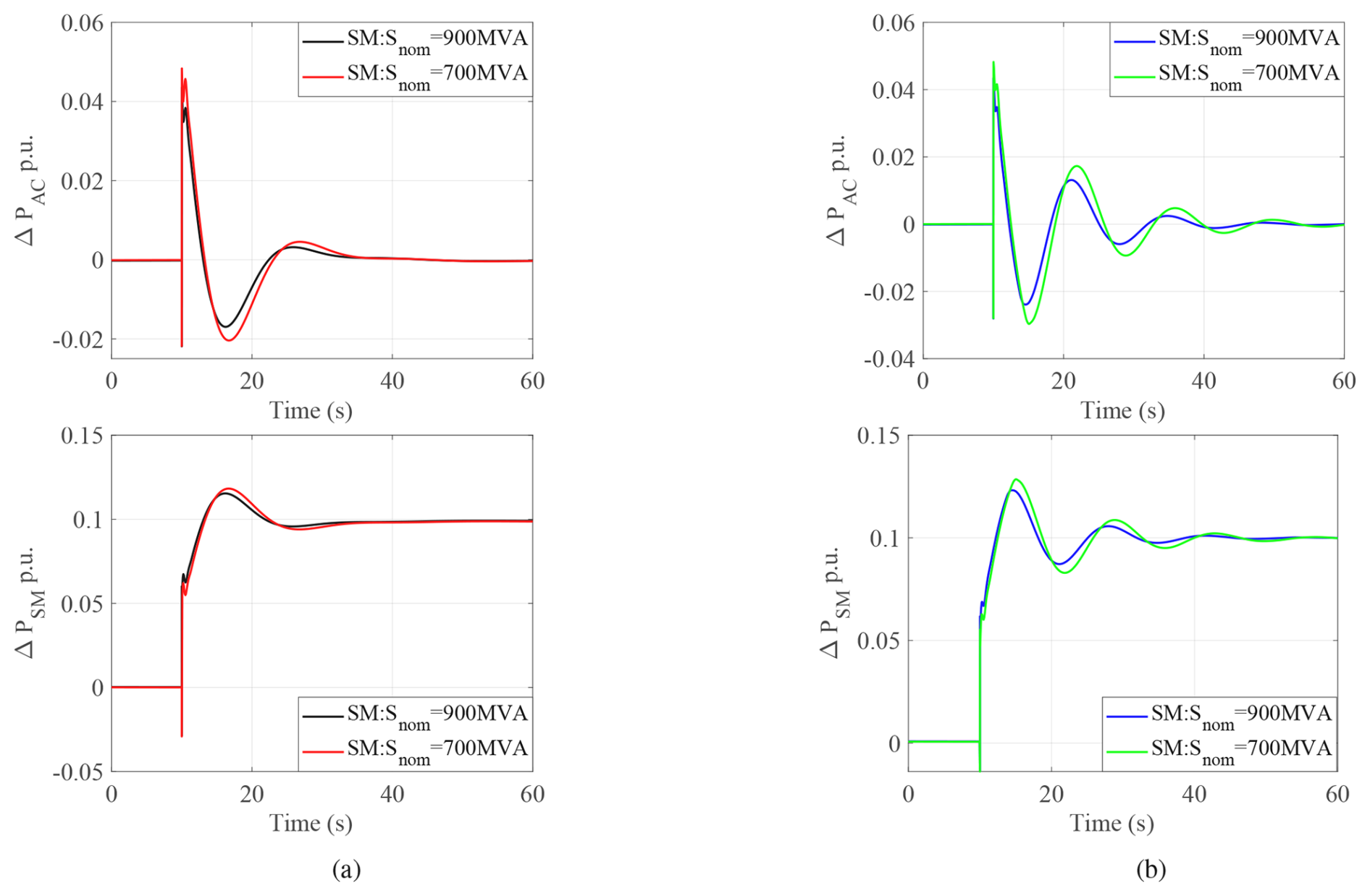
Figure 18 Comparison of system response with reduced synchronous-machine (SM) capacity for a 0.1 p.u. load step at 10 s for operating points (a) OP₁ and (b) OP₂.

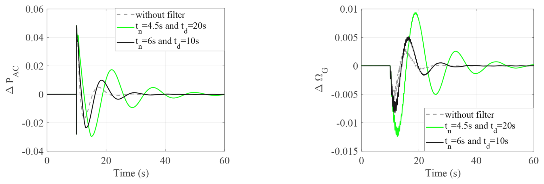
Figure 19 OP₂: response of the system for increased share of renewables with modified tuning of the lead–lag filter.

Secondly, to consider an increased share of wind farms, a reduced share of synchronous-machine investigation with a decrease in the rated capacity of synchronous machines is presented in Fig. 18. A noticeable reduction in oscillation damping is evident in the ΔΩ_G response for OP₂ as S_nom decreases. This reduction is attributed to changes in system dynamics resulting from different system parameters associated with varying S_nom. Additionally, it is observed that the damping is reduced, and it is challenging to find a good tuning of the filter due to the high gain of K_MPPT.

An analysis with different tuning of the lead–lag filter is shown in Fig. 19, and it is compared with the system without a lead–lag filter and with the original tuning. It is observed that with changes in wind generation, the tuning of the filter can be adjusted, which leads to good damping characteristics of the system. However, this adjustment leads to a reduction in the inertial response, as seen from ΔP_AC. The modification of filter parameters leads to the recovery of the coupling between the wind turbine and the grid-forming converter, as observed from the system response, which is closer to the case without a filter after tuning. This is also evident from the closer values of t_n and t_d, which results in a weaker lead effect. Therefore, depending on the application, it is a trade-off between the requirement of the initial effect and the damping of the system.

5 Conclusions

The simplified model proposed in this paper highlights the new coupling due to the requirement for grid-forming behavior in wind turbines. This model provides a clear understanding of how the dominant frequency mode is influenced by wind turbine dynamics and identifies the key parameters that affect this mode. Among these, the gain of the MPPT (maximum power point tracking) strategy emerges as a critical factor, as its value varies significantly depending on the operational zone.

Additionally, the analysis also underscores the importance of accounting for the internal mechanical dynamics of the wind turbine. Depending on the operating point, unwanted oscillations can appear in the rotational speed of the turbine. To address this, an active damping effect can be introduced to suppress oscillatory mechanical modes by incorporating an input-shaping filter to generate the active power reference. This approach is advantageous compared to previously proposed methods, as it avoids interference with the DC bus control dynamics and has a negligible impact on the active power dynamics of the wind turbine. It has also been further revealed that the internal dynamics of the wind turbine influence the dominant frequency mode. This is due to the interaction between the MPPT control and active power management, as rapid modifications of the power reference reduce the expected inertial effect of the grid-forming converter.

A practical solution to mitigate this issue is the addition of a filter in the control loop. In this case, the filter is of a lead–lag type, which serves to decouple the system's dominant mode from the mechanical modes of the wind turbine. As expected, mechanical variations are more pronounced on the wind turbine side, where energy exchange with the grid is higher. This paper has outlined general trends in the dynamics of grid-forming wind turbines connected to an AC grid; however, further work is needed to deepen this analysis. The proposed solution decouples the inertial effect provided by the wind turbine and the grid-forming converter, but there is a limitation to using this inertia as it is against the natural behavior of the system. To address this undesired coupling, a more advanced control strategy can be implemented to achieve effective dynamic decoupling. The mechanical model should be improved to ensure that the unmodeled modes do not induce additional interaction with the grid modes. Moreover, it is possible to implement other types of MPPT control and analyze if the same conclusion can be drawn.

Appendix A: Parameters of the system

Table A1 System parameters.

Table A2 Wind turbine grid-forming parameters.

Table A3 Synchronous-machine parameters.

Table A4 Filter parameters.

Table A5 List of abbreviations.

Table A6 List of nomenclature.