Characterization of HRRR-simulated rotor layer wind speeds and clouds along the coast of California

Stratocumulus clouds, with their low cloud base and top, affect the atmospheric boundary layer wind and turbulence profile, thereby modulating wind energy resources. GOES satellite data reveal an abundance of stratocumulus clouds in the late spring and summer months off the coast of northern and central California, where there are active plans to deploy floating offshore wind farms at two lease areas (near Morro Bay and Humboldt). Since the fall of 2020, two buoys equipped with multiple instruments, including Doppler lidar, have been deployed for about 1 year in these wind farm lease areas to assess the rotor layer wind conditions in these locations. The objective of this study is to evaluate how well the High-Resolution Rapid Refresh (HRRR) model represents stratocumulus cloud characteristics and turbine-relevant rotor layer winds (surface to 300 m) by comparing HRRR simulations with buoy and satellite observations. We first find that the HRRR model reproduces the seasonal cycle of cloud top height reasonably well in these regions. However, during the warm season – especially at Morro Bay – the HRRR-simulated stratocumulus clouds tend to have lower tops by about 150 m and exhibit weaker diurnal cycles than satellite observations. Our analysis also shows that rotor layer wind speeds and vertical shear are stronger at Humboldt than at Morro Bay, and both are generally stronger under clear-sky conditions. Finally, the HRRR model bias in rotor layer wind speed is small under cloudy conditions but larger and dependent on observed wind speed under clear skies. Specifically, HRRR underestimates wind speeds at Morro Bay and overestimates them at Humboldt under clear-sky conditions.

1 Introduction

Due to the semi-permanent Pacific high-pressure system and cold sea surface temperatures (SSTs) from coastal upwelling, marine boundary layer clouds appear frequently off the coast of California year-round (Iacobellis and Cayan, 2013; Lin et al., 2009). During the warm season in particular, marine stratocumulus and stratus (from here on, stratocumulus) are most pronounced. These clouds originate in subsiding dry and warm air as the high-pressure system interacts with the cold, humid, and shallow marine atmospheric boundary layer (MABL), forming a stronger capping inversion. The capping temperature and moisture inversion limit the vertical extent of the low-level clouds. Marine stratocumulus clouds are shallow (∼ 200 m thickness) but optically thick, therefore inducing radiative cooling at the top of the boundary layer, primarily in the longwave spectrum. Cloud top radiative cooling, along with surface buoyancy production, cloud top entrainment, and wind shear, drives the turbulence in the MABL and hence the cloud and precipitation processes. As turbulence and cloud processes are intimately coupled in the MABL, the presence of marine stratocumulus affects the profile of winds and turbulent properties within the marine boundary layer (Wood, 2012).

Recent modeling and observational studies have provided deeper insight into the physical processes governing the stratocumulus-topped boundary layer (STBL). In particular, Kopec et al. (2016) investigated how radiative cooling at the cloud top and wind shear across the capping inversion jointly influence turbulence generation and cloud top structure using large-eddy simulations based on the POST field campaign. Their analysis demonstrated that radiative cooling intensifies convective circulations within the STBL, while wind shear enhances turbulence and mixing in the inversion layer above the cloud, often producing a distinct turbulent sublayer that is dynamically decoupled from the convective motions below. These findings highlight the importance of representing both shear- and radiation-driven turbulence for accurate modeling of stratocumulus dynamics and their influence on boundary layer winds. Such processes are particularly relevant for offshore wind resource assessment, where low-level clouds modulate turbulence and wind shear within the turbine rotor layer.

In July 2005, the Marine Stratus/Stratocumulus Experiment (MASE) field campaign was carried out off the coast of Monterey (California) to sample clouds and aerosols (Lu et al., 2007). Measurements including cloud base and top heights were conducted from research flights 13 different times. Out of those measurements, cloud base height varied between 67 and 315 m, and cloud top height ranged from 268 to 732 m. These measurements indicate that all or a lower portion of marine boundary layer clouds can exist at the wind-turbine-relevant height near the coast of California in summertime. Therefore, it is important to evaluate the influence of marine boundary layer clouds on the wind resources off the coast of California (Shaw et al., 2022).

Off the coast of California, there are active plans to deploy offshore wind farms at two lease areas, one along northern California near Humboldt Bay and another along central California near Morro Bay. Starting in October 2020, Doppler-lidar-equipped buoys that are owned by the United States Department of Energy (DOE) were deployed to continuously measure wind speed at various heights below 240 m for 1 year (Krishnamurthy et al., 2023). This dataset provides a unique opportunity to evaluate the performance of numerical weather prediction (NWP) models at the planned wind farm locations. Sheridan et al. (2022) utilized this dataset to assess the bias in hub-height wind speed using various reanalysis and NWP model data. They also investigated potential relations between the bias in terms of atmospheric stability and shear strength. However, they did not consider the influence of MABL clouds as a source of model bias in the hub-height wind speed. Additionally, their analysis did not include an evaluation of winds simulated by the High-Resolution Rapid Refresh (HRRR) model, despite HRRR being one of the most widely utilized forecasting tools for evaluating skill in representing rotor layer wind conditions over the United States.

Several prior studies have evaluated the HRRR model with respect to hub-height wind speed assessment. Liu et al. (2025) benchmarked hub-height wind speeds from HRRR analyses against multi-source observations across the southeastern United States and found that wind speed biases were strongly influenced by local topography and land surface characteristics such as forest canopy height. Complementary efforts under the Second Wind Forecast Improvement Project (WFIP2) assessed experimental updates to the HRRR model using scanning Doppler lidar measurements in the complex terrain of the Columbia River basin (Pichugina et al., 2020). That study demonstrated that the HRRR model's wind speed errors were the largest below about 150 m above ground level and that improvements in model physics and grid resolution led to modest but consistent reductions in mean wind speed bias. Together, these findings highlight the importance of evaluating HRRR's performance in diverse environments, including offshore regions where boundary layer cloud processes can further influence rotor layer winds.

The aim of this study is to compare the modeled (HRRR) and observed (satellite and buoy) characteristics of stratocumulus clouds and winds at turbine-relevant heights and assess the HRRR's bias in wind speed near the surface for better decision-making in wind farm development off the coast of California. The paper is organized as follows. Section 2 provides a brief description of the various datasets used in this study and how they were post-processed to allow direct comparisons. The characteristics of clouds, hub-height wind speed, and model wind bias in relation to cloud properties at the Humboldt Bay and Morro Bay locations are explored in Sect. 3. A summary and conclusions follow in Sect. 4.

2 Data and methods

2.1 Lidar-buoy observation dataset

DOE-owned buoys with multiple instrumentations were deployed about 40–50 km off the coast of Morro Bay (35.71074° N, 121.84606° W) and Humboldt (40.9708° N, 124.5901° W). Each of the buoys started the operation in the fall of 2020, and the mission lasted about 1 year. In December 2020, a significant wave event at the Humboldt buoy location caused a power outage, resulting in a substantial data gap. The buoy equipment was restored and brought back online on 25 May 2021. Details about the instruments on the buoys and the methods for the raw data processing can be found in Krishnamurthy et al. (2023).

The buoys were equipped with WindCube 866 Doppler lidar to measure the vertical profiles of motion-compensated wind speed at 1 s temporal resolutions. The final post-processed wind profiles are at 10 min temporal resolution with 10 m range resolution from 40 to 240 m above the surface. The buoys were also equipped with an LI-200SA pyranometer (PYR) to measure the global broadband solar radiation at 10 min temporal frequency. By comparing the measured solar radiation to the modeled solar radiation for clear-sky conditions, we determined whether cloud presence attenuated the downwelling solar radiation reaching the surface (Long and Ackerman, 2000). The temporal cloud mask, which provides a time series of sky conditions, was derived by quantifying the deviation between the observed and modeled clear-sky solar radiation. When the measured radiation was more than 10 % lower than the modeled clear-sky value, the condition was classified as cloudy. Otherwise, it was designated as cloud-free (Krishnamurthy et al., 2023).

2.2 Cloud top height from GOES

Cloud top heights over our study duration were taken from the Satellite ClOud and Radiation Property Retrieval System (SatCORPS) Clouds and the Earth's Radiant Energy System (CERES) Edition 4 (Ed4) Geostationary Operational Environmental Satellite (GOES) record (Minnis et al., 2021). This record, with ∼ 8 km spatial resolution and hourly cloud property retrievals, is prepared by NASA SatCORPS through the processing of GOES-15, GOES-16, and GOES-17 geostationary imagers belonging to the GOES program (Menzel and Purdom, 1994). For this study, GOES-17 is the only satellite providing data that overlaps with the buoy observation period. These retrievals use the CERES Ed4 algorithms, adapted for geostationary applications. These Ed4 algorithms and their nominal quality assessments can be found in Minnis et al. (2021). Since these retrievals from geostationary satellites are not provided over a fixed spatial grid, we prepared a time series of hourly retrievals that were closest to the buoy locations (Sect. 2.1). From here on, we simply refer to this record as GOES.

GOES determines cloud top height (CTH) from infrared-retrieved cloud top temperature (CTT) and lapse-rate calculations following Sun-Mack et al. (2014). The CTT measurements have an accuracy of about 1 K (Yu et al., 2013), which corresponds to an uncertainty of roughly 100 m in CTH for a dry-adiabatic lapse rate. Previous studies have shown that inaccuracies in lapse-rate estimates can lead to CTH errors of this magnitude (Zuidema et al., 2009; Ghate et al., 2019). Comparisons of the most recent SatCORPS Edition 4 GOES retrievals with CloudSat and CALIOP indicate mean differences near 100 m (Yost et al., 2021). A recent 7-year analysis comparing ERA5 and GOES data reported ERA5–GOES differences of −0.17 ± 0.62 km (Humboldt) and −0.22 ± 0.51 km (Morro Bay) (Mitra et al., 2025). These results imply that GOES retrieval uncertainties are of the order of 100–200 m – smaller than the HRRR–GOES differences reported here – and that the HRRR bias in CTH likely reflects model limitations rather than retrieval limitations.

Instances of multilayer cloud systems (e.g., thin cirrus overlying low stratocumulus) were handled by filtering out retrievals with cloud top heights exceeding our low-cloud thresholds. In such cases, the GOES infrared retrieval reports the upper-level cirrus as the primary cloud top, leading to spuriously high CTH values that are automatically excluded from the analysis. Situations with optically thick cirrus that fully obscure the low-level cloud deck are likewise classified as high-cloud conditions and are not used when evaluating boundary layer properties or HRRR wind speed biases.

2.3 High-Resolution Rapid Refresh (HRRR) v4

HRRR is a 3 km spatial resolution, hourly updating, convection-permitting atmospheric forecast model developed and operated by the National Oceanic and Atmospheric Administration (NOAA) (Dowell et al., 2022). HRRR provides high-fidelity short-term atmospheric forecasting and provides the meteorological variables necessary for wind power estimation and forecasting applications. HRRR's initial conditions are generated from the parent Rapid Refresh (RAP) model 1 h prior to forecast initialization. RAP forecast is advanced forward, assimilating the most recent observations to provide a dynamically consistent state for HRRR initialization. Lateral boundary conditions for HRRR are supplied by the RAP model at 3 h intervals. HRRR employs a hybrid ensemble-variational (EnVar) data-assimilation system that integrates a 36-member ensemble to represent flow-dependent background errors. The assimilation cycle updates every hour and incorporates a wide range of conventional, satellite, and radar observations. Within each cycle, radar reflectivity and radial-velocity data are assimilated every 15 min to improve the representation of cloud and convective structures. Surface and soil states are updated using short-term forecasts from the HRRR Data Assimilation System (HRRRDAS), which maintains temporal continuity between analysis cycles. This framework is designed to minimize spin-up errors and improve the depiction of boundary layer and mesoscale processes critical to wind forecast applications. We use data from HRRRv4, which was released in December 2020, and its data availability aligns with our buoy observation period. We utilize HRRR 3 h forecast data that output wind speed at the native model vertical grid. By comparing the model's vertical grid with the lidar buoy's measurement height, we determine that the first four of the model's vertical height levels are close to the heights of 40, 80, 160, and 240 m, at which data from lidar measurement are available. The HRRR-reported wind profiles were linearly interpolated to obtain wind speeds at 40, 80, 160, and 240 m. We extract the data from the point closest to the buoy locations, which is not farther away than 1.4–2.5 km on average. We compute the wind speed bias by subtracting buoy-reported wind speed from that reported by HRRR at 40, 80, 160, and 240 m. Because HRRR outputs are available only at full-hour intervals, we selected the 10 min averaged lidar measurements whose timestamps correspond exactly to each forecast hour, ensuring consistent temporal alignment between the HRRR time series and the buoy observations.

3 Results

3.1 Characteristics of clouds off the coast of California

Figure 1a and b present the distribution of cloud top heights computed by HRRR and estimated by GOES for each month of the observation period, and Fig. 1c and d show the same for cloud fraction. There are significant seasonal changes in cloud top heights and cloud fraction at both the Morro Bay and the Humboldt locations. For Morro Bay, cloud fraction values from both HRRR and CERES exceed 80 % consistently between May and September. In contrast, Humboldt Bay exhibits greater month-to-month variability in cloud fraction, with summer months not necessarily showing high values. The low cloud top heights (<3 km) and high cloudiness between April and October suggest the clouds to be low-level marine stratocumulus clouds, while higher cloud top heights (>7 km) and low cloudiness during the colder months suggest the passage of mid-latitude frontal systems, consistent with Lin et al. (2009). Overall, the winter months have higher cloud top heights than the summer months at both locations. This seasonal variation in cloud top height is accurately captured by the HRRR model. However, there are some minor discrepancies between the median values of observed and HRRR-simulated cloud top heights. The quartile ranges and median values of cloud fraction reveal discrepancies between CERES and HRRR, with the differences being particularly pronounced for Humboldt Bay. These differences may partly reflect the distinct definitions of clouds used in the two datasets. The GOES retrieval identifies a cloud layer only when the optical depth exceeds a threshold that varies with viewing geometry and atmospheric conditions, while HRRR defines clouds based on the simulated presence of hydrometeors within model grid cells. Because no satellite instrument simulator was applied to the HRRR output, such definition and sensitivity differences might contribute to the observed discrepancies in cloud top height and cloud fraction.

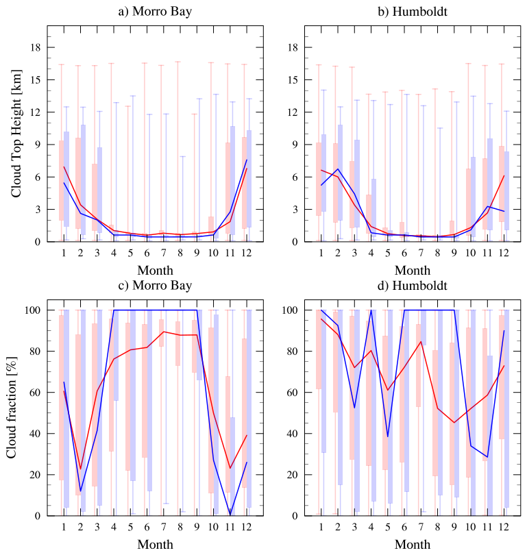
Figure 1 Box plot of (a, b) cloud top height from GOES (red) and HRRR (blue) and (c, d) cloud fraction from CERES (red) and HRRR (blue) for each month of the observation period at (left column) Morro Bay and (right column) Humboldt. The box represents the 25th and 75th percentiles, and the bounding lines represent the minimum and maximum values. Median values are represented by thick lines.

As we are interested in investigating the HRRR bias when low-altitude clouds interfere with the rotor layer, the rest of the analysis only uses data from the warmer months. Guided by Fig. 1, the data from May to the end of September at both Morro Bay and Humboldt are composited. Due to the power outage at the Humboldt location, our results from the Humboldt site miss most of the May data.

Figure 2 shows the diurnal variation in MABL cloud top heights (cloud tops below 1.5 km) from HRRR and GOES over the warm season (May–September). On average, HRRR cloud tops are about 150 m lower than those in the GOES record at Morro Bay, while there is little difference at the Humboldt location. The mean cloud top estimated by GOES is about 700 m at Morro Bay and 520 m at Humboldt, whereas HRRR estimates a mean cloud top height of around 550 m for both locations. A clear diurnal cycle in GOES cloud top height is present at both locations, which peaks around 10:00 local time (UTC−8 h). The diurnal amplitude is larger for Morro Bay, while HRRR fails to reproduce the observed diurnal cycle at either site. Under typical marine stratocumulus conditions, cloud tops are higher at night and lower during the day due to stronger nocturnal cloud top radiative cooling. Our GOES analysis (Fig. 2) shows the opposite behavior at both sites; the reason for this discrepancy is presently unclear. The absence of a diurnal cycle in cloud top height in the HRRR model nonetheless suggests an inaccurate representation of the diurnal cycle of cloud top radiative-cooling-driven turbulence in the HRRR model.

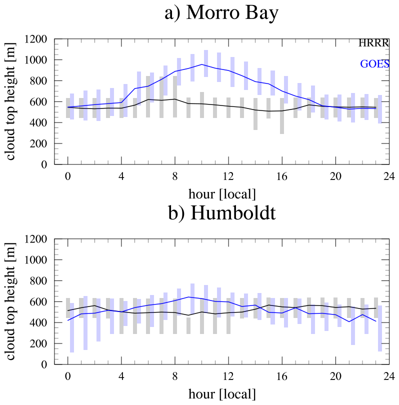
Figure 2 Warm-season (May–September) diurnal cycle of cloud top height as reported by HRRR (gray) and GOES (blue) at (a) Morro Bay and (b) Humboldt Bay. The bounding boxes represent the 25th and 75th percentiles, while the lines represent the mean values.

One likely contributing factor is the model's underrepresentation of cloud liquid water path (LWP), which cannot be directly compared with GOES in this study. A low simulated LWP would reduce the amount of shortwave absorption within the cloud during the daytime, resulting in insufficient diabatic heating and limited cloud deepening. Conversely, too little condensate would also weaken longwave cooling at night, reducing turbulent mixing at the cloud top. These combined effects could explain the muted diurnal variation in HRRR cloud top height and indicate that biases in the model's treatment of cloud microphysics and radiative processes jointly contribute to the discrepancy.

Figure S1 in the Supplement shows the percentage of clear-sky and cloudy-sky days estimated by the buoys, GOES, and HRRR between May–September at Morro Bay and Humboldt. For the buoy data, we utilize the estimated cloud mask, whereas for the HRRR and GOES datasets, the cloud mask is derived from the percentage fraction of clouds, calculated as the proportion of all hours with valid cloud top information. Out of 8547 (11 951) buoy data samples collected at Morro Bay (Humboldt) during the warm season, 2225 (4529) were classified as clear sky, while 6322 (7422) were classified as cloudy. Figure S1 indicates that during the warm season when marine stratocumulus clouds are most pronounced, cloudy days are dominant off the coast of California, and Morro Bay is cloudier than Humboldt, which is consistent with the finding in Krishnamurthy et al. (2023). The HRRR-estimated cloud fraction slightly underestimates the buoy-observed cloud fraction, which is less than 10 %, but is generally in good agreement with other sources of observation (GOES and buoy).

Throughout this study, we investigate the HRRR bias in rotor layer wind speed in terms of cloudy days versus clear-sky days. Unless specified otherwise, only warm-season (May–September) data are considered in this study. Additionally, we select a few case studies of marine stratocumulus clouds later in Sect. 3.4 to investigate the model performance.

3.2 Variation in rotor layer wind speeds with cloudiness

In Fig. 3, we present the probability density function (PDF) distribution of wind speed at Morro Bay at 40, 80, 160, and 240 m heights from HRRR (panels a–c) and from the lidar buoy observation (panels d–f). We used the observed cloud mask from the buoys to distinguish between clear-sky and cloudy conditions. Rotor layer wind speeds from the lidar buoy at Morro Bay peak around 1–2 m s⁻¹ during cloudy conditions, which is below typical cut-in speeds (3–4 m s⁻¹), while they peak around 10–15 m s⁻¹ during clear-sky conditions. Additionally, the peak of the PDF shifts towards higher wind speeds under clear-sky conditions but not under cloudy conditions, suggesting the presence of wind shear during clear-sky conditions that is absent during cloudy conditions. This suggests that turbulence is forced by wind shear during cloud-free conditions, while turbulence is only forced by cloud processes during cloudy conditions due to the absence of shear. The rotor layer wind speed distributions at Morro Bay are well reproduced by the HRRR model simulations, with minor differences. The HRRR model shows a small increase in wind speeds with height during cloudy conditions at higher wind speeds, unlike the observations. During clear-sky conditions, the HRRR model does not simulate winds stronger than 25 m s⁻¹, which was reported in a few instances by the lidar.

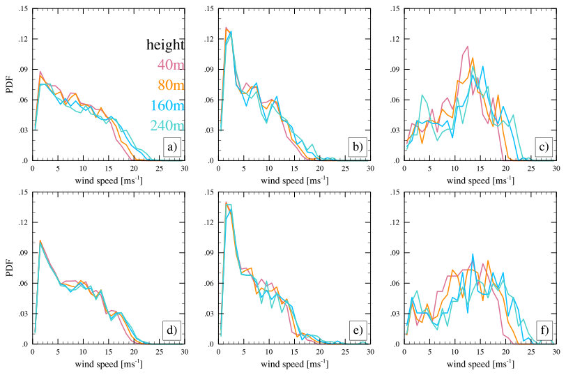
Figure 3 PDF of rotor layer (≤240 m) wind speed at Morro Bay from (top) HRRR, (bottom) the lidar buoy during (left) all conditions, (middle column) the lidar buoy during cloudy conditions, and (right column) the lidar buoy during clear-sky conditions.

Figure 4 Same as Fig. 3 but for the Humboldt location.

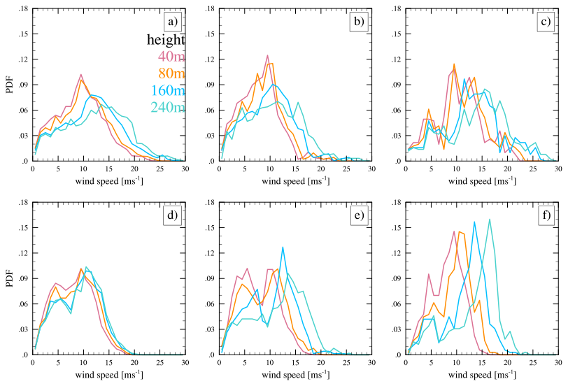
In Fig. 4, we repeated the analysis shown in Fig. 3 for the Humboldt Bay location. At Humboldt, the lidar buoy measurements of wind speed in the rotor layer show a more spread-out distribution spanning 0–20 m s⁻¹, while HRRR-reported winds range from 0 to 30 m s⁻¹. The HRRR model simulates a peak in the PDF (Fig. 4a) that shifts toward higher speeds with increasing heights, unlike what is observed (Fig. 4d). At Humboldt, strong vertical shear is present regardless of cloud conditions, as the increase in wind speed with height is evident in both datasets, but the HRRR model consistently overestimates this increase. During clear-sky conditions, the wind speed tends to be stronger compared to that under cloudy conditions, with peaks around 10–18 m s⁻¹. Collectively, the figure suggests that at Humboldt Bay, wind shear forces turbulence during both cloudy and clear-sky conditions, with the HRRR model overestimating the winds and the wind shear. However, when the shear exponent is computed directly from the mean wind speeds (Table 2), HRRR slightly underestimates the average shear compared to the buoy data. This could be because PDFs are dominated by high-wind events, which amplify apparent vertical gradients, while the mean shear exponent integrates over all wind speed regimes and may therefore show weaker shear on average.

According to Table 1, the mean 80 m wind speed at Humboldt Bay is stronger than that at Morro Bay, regardless of weather conditions. The hub-height wind speed is stronger under clear-sky conditions at both locations compared to that during cloudy conditions. We can relate clear-sky conditions to stable stratification in the atmospheric boundary layer. Under stable stratification, the surface layer – approximately 10 % of the atmospheric boundary layer – becomes shallower in the marine boundary layer. This shallowness traps surface turbulent fluxes within the surface layer and decouples them from the layer above, leading to stronger wind speeds (Mahrt, 1999). These decoupled boundary layers are known to have lower cloudiness and higher winds than coupled boundary layers (e.g., Serpetzoglou et al., 2008, and Jones et al., 2011). The average wind speed difference between cloudy and clear-sky conditions is stronger at Morro Bay, within both the buoy and the HRRR records. During cloudy conditions, the HRRR wind speed is comparable to the observed hub-height wind speed. During clear-sky conditions, HRRR underestimates the hub-height wind speed at Morro Bay, while it overpredicts it at the Humboldt location.

Table 1 Mean ± standard deviation of wind speed of the lidar buoy observation and HRRR at 80 m height for cloudy and clear conditions.

Table 2 Mean ± standard deviation of the wind shear exponent α of the lidar buoy observation and HRRR for cloudy and clear conditions.

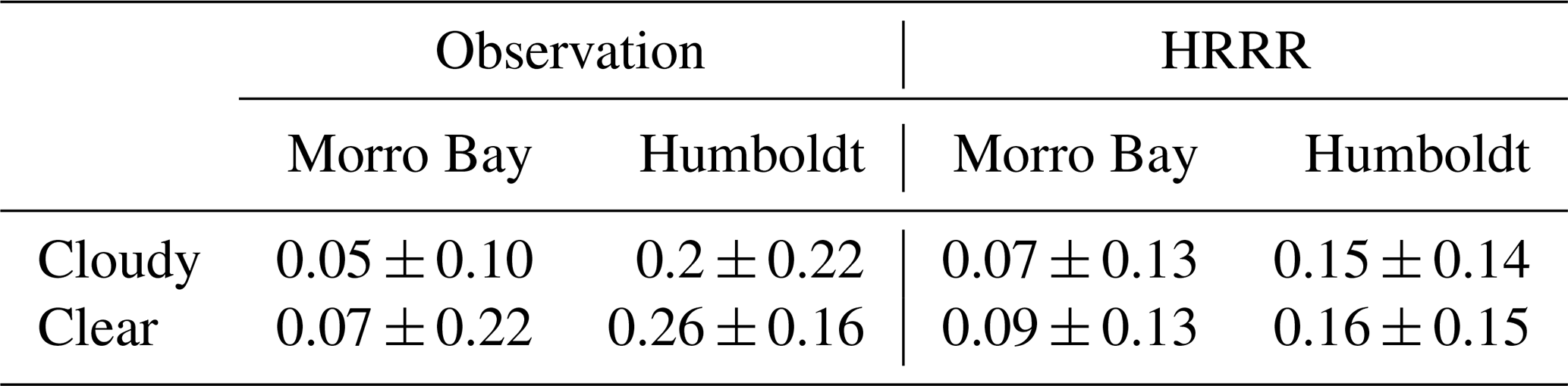
Table 1 further demonstrates that the standard deviation of 80 m wind speed during cloudy conditions is comparable between the observations and HRRR at both locations. However, notable differences are observed under clear-sky conditions.

Following Wharton and Lundquist (2012), we compute the wind shear exponent α following

$$\begin{array}{}\text{(1)}& \mathit{\alpha }={\displaystyle \frac{\ln (v_{\mathrm{2}}/v_{\mathrm{1}})}{\ln (z_{\mathrm{2}}/z_{\mathrm{1}})}},\end{array}$$

where v₂ is the wind velocity at height z₂, and v₁ is the wind velocity at height z₁. For this analysis, we set z₂=160 m and z₁=40 m. Table 2 lists α values using the lidar buoy observations and HRRR for Morro Bay and Humboldt under cloudy and clear conditions. As mentioned earlier, α confirms that the shear is about 4 times stronger at Humboldt regardless of weather conditions. Stronger shear at Humboldt is also evident in the vertical profile of the lidar buoy wind speeds shown in Krishnamurthy et al. (2023). Under stable stratification, the surface layer is accompanied by weak turbulence, which allows stronger shear and veer to develop. Consistently, in both locations, shear is stronger under clear-sky conditions. The shear exponent is underestimated in HRRR at the Humboldt location, while it is overestimated at Morro Bay. A previous modeling study by Zamora Zapata et al. (2021) showed that cloud fraction decreases with an increase in near-surface wind shear. Their results are consistent with our finding that cloud fraction in Humboldt (with stronger shear) is lower than in Morro Bay (Fig. 1).

3.3 Characteristics of hub-height wind speed bias in terms of cloudiness

Figure 5 shows the distribution of 80 m wind speed bias in HRRR, binned by observed wind speed. Prior to binning, data were separated by their weather conditions (i.e., total, cloudy, and clear sky). The median difference between the observed and modeled winds is less than 1 m s⁻¹ at both locations, while the range of the differences is higher at Morro Bay compared to Humboldt Bay. At Morro Bay, the range of the bias across all observed wind speeds remains between ± 5 m s⁻¹, while this range is higher at Humboldt Bay. At Morro Bay, HRRR is largely unbiased for wind speeds below 10 m s⁻¹ but consistently underestimates the observed hub-height wind speed under cloudy conditions when wind speeds exceed this threshold, with the magnitude of underestimation increasing at higher wind speeds. During weak- to moderate-wind-speed events (0–10 m s⁻¹), the HRRR model slightly overestimates wind speed under clear-sky conditions, and the bias sign then changes as the observed wind speed is beyond 10 m s⁻¹. The change in bias from positive to negative with an increase in wind speed is the strongest under clear-sky conditions. The wind speed biases at Morro Bay during the warm season are similar to those reported by Sheridan et al. (2022).

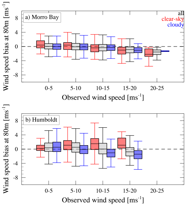
Figure 5 Box-and-whisker plot of wind speed bias at 80 m between HRRR and lidar (HRRR and lidar) at various observed wind speeds for clear-sky (red), all (grey), and cloudy (blue) conditions at Morro Bay (top) and Humboldt Bay (bottom).

At Humboldt, HRRR slightly overestimates the hub-height wind speed when the observed wind speed is weak (0–5 m s⁻¹), regardless of weather conditions. However, unlike Morro Bay, the median HRRR bias for hub-height wind speed under clear-sky conditions remains positive even during strong-wind-speed events, while it changes to negative under cloudy conditions. Similar to Morro Bay, the bias under clear-sky and cloudy conditions increases with higher observed wind speed. Because of the opposing bias signs between clear-sky and cloudy conditions at Humboldt, the median HRRR bias in hub-height wind speed over the entire period is close to zero. Our results are consistent with the findings in Sheridan et al. (2022), where the hub-height wind speed bias was investigated in terms of atmospheric stability. In Sheridan et al. (2022), the results of the Rapid Refresh (RAP) model indicated an overestimation of wind speed at Humboldt in stable conditions, while the bias flipped its sign under unstable conditions. In their analysis, Morro Bay showed an underestimation of wind speed regardless of the stability condition when RAP was compared to the lidar buoy observation. In both locations, the bias was much larger during stable conditions, where the development of clouds is discouraged. However, we did not find any meaningful correlation between the SST bias and wind speed bias when examining the relationship over the entire period, as well as separately for cloudy conditions, clear-sky conditions, and stable atmospheric cases.

We repeated the analysis shown in Fig. 5 for the entire period of available observation data (not shown). For Morro Bay, entire-year data are utilized. For Humboldt, the period from December 2020 to May 2021 was excluded due to the unavailability of data. The analysis of the wind speed bias for the longer period is consistent with that for warmer months.

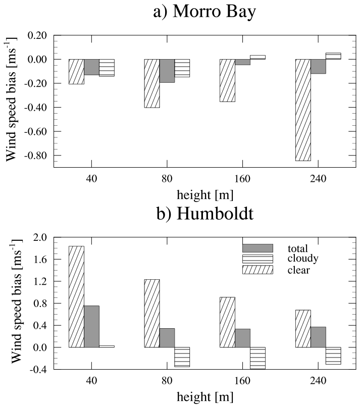
Figure 6 Mean wind speed bias (HRRR and lidar) for all weather conditions in the warm season (grey box), clear-sky conditions (slanted stripes), and cloudy conditions (horizontal stripes) at various heights below 240 m.

Next, we demonstrate how the mean wind speed bias changes with height (Fig. 6). At Morro Bay, HRRR underestimates the magnitude of low-level wind speed under all weather conditions, with the bias being most pronounced under clear-sky conditions. The underestimation of wind speeds by the HRRR model increases with height, with a value of −0.8 m s⁻¹ at 240 m. The HRRR model simulates winds fairly accurately during cloudy conditions at Morro Bay.

At Humboldt Bay, the HRRR model overestimates rotor layer wind speeds during clear-sky conditions and underestimates them under cloudy conditions. The overestimation of winds during clear-sky conditions decreases with height from 40 to 240 m. Humboldt Bay experiences higher wind shear than Morro Bay. The HRRR model overestimates wind speeds during clear-sky conditions at Humboldt Bay and underestimates them at Morro Bay. This suggests that the model has difficulty in accurately simulating wind shear in clear-sky situations, tending to overestimate winds when shear is strong and underestimate winds when shear is weak. Although this bias is much smaller during cloudy conditions, the HRRR model still overestimates wind speeds at Morro Bay and underestimates them at Humboldt Bay.

As discussed by Optis et al. (2016) and references therein, similarity-based wind speed profile formulations derived from the Monin–Obukhov similarity theory (MOST) can exhibit substantial bias under strongly stratified boundary layers. Because HRRR employs surface layer and turbulence parameterizations that draw from this theoretical framework, such limitations may contribute to the under- or overestimation of wind speeds observed under stable, clear-sky conditions in our analysis. It should be noted, however, that HRRR applies MOST primarily within the surface layer, while turbulent mixing above this layer is represented using an eddy-diffusivity mass-flux (EDMF) approach that accounts for nonlocal transport and convective plumes (Olson et al., 2019a, b). Optis et al. (2016) demonstrated that wind speed bias at 40, 80, 140, and 200 m heights increased with the strength of stratification and even changed sign under different stratification regimes. Although informative, their results cannot be directly extrapolated to offshore regions with high cloudiness, such as those studied here. Over land, boundary layer thermodynamic decoupling (stratification) is largely controlled by the presence or absence of surface fluxes as turbulence is primarily modulated by these fluxes. In contrast, in offshore environments with a cloud-topped boundary layer, turbulence is primarily governed by radiative cooling at the cloud top. As a result, offshore boundary layers tend to become more decoupled during the day, when cloud top cooling weakens, and more coupled at night, when radiative cooling is strongest. However, the degree of coupling can vary substantially depending on cloud optical thickness, synoptic forcing, and sea surface temperature gradients. In comparison, over land, boundary layers are typically coupled during the daytime when the surface heating is greatest and decoupled at night when the surface heating is minimal.

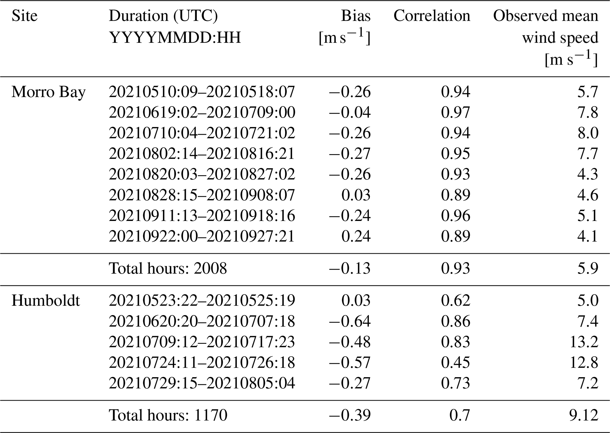
Table 3 List of stratocumulus events and their associated observed mean wind speed at 80 m, mean wind bias at 80 m, and correlation between HRRR and the lidar buoy.

3.4 Low-level wind bias with marine stratocumulus clouds

Cases of warm stratocumulus clouds were identified using the cloud top temperature data from the GOES. The cases were identified from latitude–longitude maps of visible satellite imagery and cloud top temperatures. Three objective criteria, (1) extensive cloud cover for more than 2° (∼ 200 km) in the zonal and meridional directions at the two locations, (2) cloud top temperatures in excess of 0 °C, and (3) cloud cover lasting for more than 12 h, were enforced. Most of the cases had durations exceeding multiple days. Some cases included brief breaks in cloud cover lasting less than 3 h and were therefore treated as part of the same event. Table 3 lists the duration of each identified marine stratocumulus cloud period, along with its associated 80 m wind bias, case-mean observed wind speed, and Pearson correlation coefficient. As previously discussed, hub-height wind speeds and the associated biases at Morro Bay are weaker than those at Humboldt. At both locations, HRRR generally underestimates the hub-height wind speed, except for the case in September at Morro Bay. During that event, the mean wind speed is 4.1 m s⁻¹. During weak-wind (0–5 m s⁻¹) conditions, HRRR slightly overestimates the hub-height wind speed (Fig. 5). Additionally, the correlation between the time series of lidar buoy observations and HRRR wind speed is notably weaker at Humboldt (mean correlation coefficient r=0.70) than at Morro Bay (r=0.93), highlighting regional differences in model performance.

Figure 7 presents the composite diurnal cycle of cloud top height (panels a–b), wind speed at 80 m (panels c–d), and wind bias (panels e–f) at both the Morro Bay and the Humboldt Bay locations during stratocumulus periods, listed in Table 3. At Morro Bay, GOES shows a deepening of the cloud layer in the morning, while HRRR underestimates this diurnal change. At Humboldt Bay, GOES also indicates a slight deepening of clouds in the morning. These patterns are consistent with the warm-season cloud characteristics shown in Fig. 2. Wind speed, as shown in Fig. 7c–d, exhibits a weak diurnal cycle at both locations. At Morro Bay, wind speeds peak in the evening, whereas at Humboldt, wind speeds increase at night. As indicated in Table 3, wind speeds are generally stronger at Humboldt Bay. The distribution of hub-height wind speed indicates that the bias at both locations is predominantly centered around zero. However, Humboldt exhibits a slightly greater underestimation of wind speed, which aligns with the observations presented in Figs. 5 and 6. For both Morro Bay and Humboldt, wind bias becomes positive during the nighttime. The range of the bias remains between ± 1.5 m s⁻¹ at Morro Bay, while it exceeds this range at Humboldt (not shown). It is shown in Fig. 6 that stronger wind speed induces stronger bias.

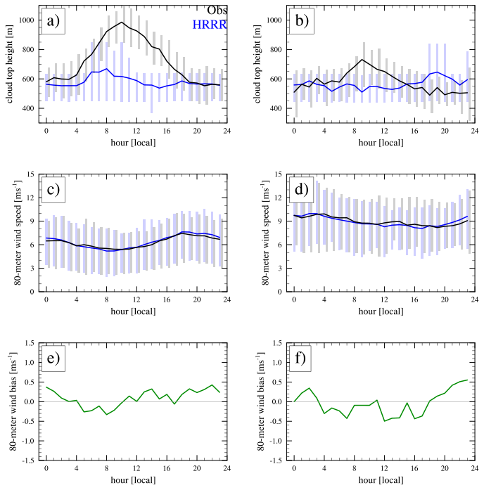
Figure 7 Composite diurnal cycles of (a–b) cloud top height, (c–d) wind speed at 80 m height, and (e–f) wind speed bias between the lidar observation and HRRR during the stratocumulus periods listed in Table 3. The left column represents Morro Bay, and the right column represents Humboldt. The bar represents the 25th and 75th percentiles, while the line represents the mean. The black lines represent GOES satellite data for cloud top height and lidar data for wind speed, while the blue lines represent HRRR results. The green lines are directly computed as the difference between the black and blues lines in (c) and (d).

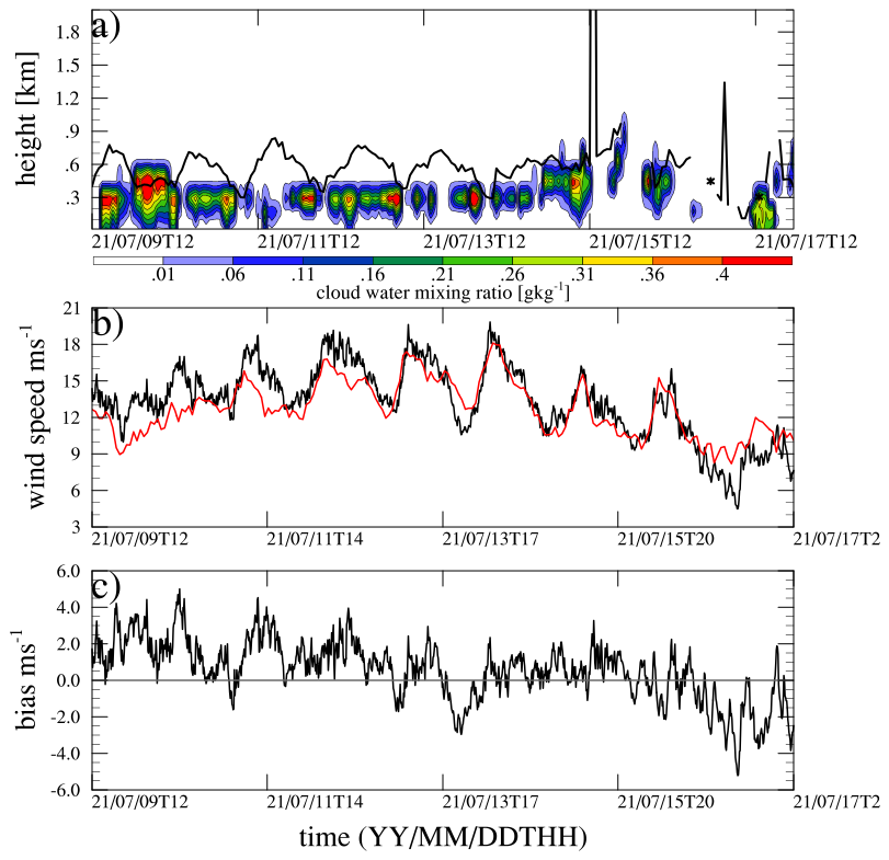
Figure 8 (a) Time series of HRRR-simulated cloud water mixing ratio (contour) and GOES-reported cloud top height (black line), (b) time series of wind speed at 80 m observed by the lidar buoy (black) and modeled by HRRR (red), and (c) time series of wind speed bias (lidar and HRRR) at 80 m. The location is Humboldt.

In Fig. 8, we closely examine the cloud top height and hub-height wind speed during one of the stratocumulus periods listed in Table 3. Figure 8a shows the time series of the vertical profile of the cloud water mixing ratio simulated by HRRR, alongside the cloud top height estimated by GOES. As shown in Sect. 3.1, HRRR-simulated cloud tops are lower than the GOES-estimated values. While there is no clear indication of a diurnal cycle in cloud top height at Humboldt (Fig. 2b), during this particular period (9–17 July 2021), GOES cloud top data show a strong diurnal cycle for the first 5 d. In the observations, clouds are in the form of long-lived sheets, while clouds simulated by HRRR are mostly intermittent, as indicated by the gaps in the cloud water mixing ratio. It is important to note that Fig. 8a shows only the resolved cloud liquid water mixing ratio fields from HRRR. The operational HRRR output does not include subgrid-scale cloud liquid water, and therefore the figure cannot represent partially cloudy grid cells where unresolved cloud condensate may be present. As a result, some of the apparent “gaps” in the HRRR cloud field may in fact contain subgrid-scale cloud liquid that is not captured in the resolved output. We also compare the 80 m wind speed between the lidar buoy observation and HRRR simulation. During this stratocumulus period, wind speed consistently exceeds the cut-in speed and occasionally surpasses the rated speed. The observation reveals a very strong diurnal cycle in hub-height wind speed, which HRRR reproduces well in terms of amplitude and phase. However, both positive and negative bias exists in HRRR during this period, but the underestimation during the first 4 d outweighs some periods of overestimation (Fig. 8c). The diurnal cycle of the wind speed bias and the diurnal cycle of the GOES-reported cloud top height suggest the bias to be related to the cloud-modulated turbulence in the boundary layer.

4 Summary and conclusion

Marine stratocumulus clouds are shallow and located below the capping marine boundary layer inversion. The radiative cooling at the cloud top often generates turbulence mixing downward, which can modulate the PBL turbulence profile (Wood, 2012). Moreover, the radiative cooling at the cloud top can strengthen the capping inversion, which can generate shear at the inversion layer. This shear is known to initiate atmospheric waves, which can adjust the wind speed and turbulence intensity within the marine boundary layer (Allaerts and Meyers, 2018). Therefore, a better understanding of the processes within the marine boundary layer bounded by marine stratocumulus clouds is important to better assess and predict wind conditions in coastal regions dominated by these clouds (Shaw et al., 2022).

There are wind farm lease areas off the coast of northern and central California (Musial et al., 2019) where marine stratocumulus clouds are abundant during warmer months (Wood, 2012). In the fall of 2020, two DOE buoys with multiple instruments, including Doppler lidar and pyranometers, were deployed to these lease areas (Humboldt and Morro Bay locations) for about a year to continuously measure the vertical profile of wind speed below 240 m and global broadband solar radiation, among other factors. The presence of this dataset, in combination with GOES satellite data, provides a unique opportunity to assess the HRRR model bias in forecasting wind speed in rotor-layer-relevant heights in terms of cloudiness. The primary findings of this work are as follows.

Consistent with previous studies, GOES satellite data indicate that marine stratocumulus clouds are prevalent at both locations during the warmer months. Cloud cover is greater at Morro Bay compared to Humboldt Bay, and Morro Bay also exhibits a more pronounced diurnal cycle in cloud top height. Overall, the HRRR model captures the general cloudiness well but underestimates both the cloud top heights and the amplitude of the diurnal cycle at both sites, with the underestimation being especially pronounced at Morro Bay.

Wind speeds and shear within the rotor layer are stronger at Humboldt Bay than at Morro Bay. At both locations, rotor layer wind speeds and shear are higher on clear-sky days compared to cloudy days. The HRRR model generally reproduces these patterns, although some biases remain.

At both locations the HRRR model tends to underestimate the 80 m wind speed in cloudy conditions (with a median bias of −1.5 m s⁻¹), and this negative bias increases with higher wind speeds. Under clear-sky conditions, the wind speed bias is larger, with the model overestimating wind speeds at Morro Bay (positive bias) and underestimating them at Humboldt Bay (negative bias).

Under cloudy conditions, the mean wind speed bias at different heights (40, 80, 160, and 240 m) is generally small, close to zero, or shows slight underestimation by the model. Under clear-sky conditions, the opposite bias pattern between Humboldt Bay and Morro Bay remains consistent at all rotor layer heights.

Stratocumulus cloud events at Morro Bay and Humboldt Bay during warmer months were identified by visually inspecting GOES images. Those specific stratocumulus events also reveal that mean wind speed and wind speed bias are stronger at Humboldt Bay. In both locations, the mean bias is negative.

Due to the shallow depth of the marine boundary layer, the top of the surface layer, where the Monin–Obukhov (M–O) similarity theory is applicable, could be close to the wind turbine rotor layer. Moreover, the M–O similarity theory is strongly dependent upon atmospheric stability. Many studies have shown that the M–O similarity theory does not work very well above the surface layer and under stable stratification. This may explain why the HRRR bias is stronger under clear-sky conditions. The different HRRR bias sign at the two locations under clear-sky conditions may be related to the strength of atmospheric stability. Further measurements, such as those of the boundary layer thermodynamic profile, would be required to verify this theory.

Our analysis uses data only for the May to September time period because that is when marine stratocumulus clouds are most abundant in the region. When we include the entire data period, including colder months, we obtain very similar results, as shown in Fig. 6, even though the data period from December to May is missing for the Humboldt location: (1) bias is larger under clear-sky conditions than in cloudy conditions, and (2) the bias sign under clear-sky conditions is the opposite between Humboldt and Morro Bay. Although the fraction of clear-sky days is much lower compared to the cloudiness fraction during warmer months, in colder months, the fraction of clear-sky days increases (not shown). Therefore, it is equally important to improve HRRR model physics to better represent marine boundary layer processes under clear-sky (stable) conditions.

Lastly, in this article we characterized the biases in the HRRR-model-simulated rotor layer winds and clouds. Broadly, the analysis shows the wind speed biases to differ between cloudy and clear-sky conditions and significant bias in the HRRR-simulated cloud fraction and cloud top heights. The turbulence in the cloud-topped boundary layers is modulated by cloud processes, which then in turn affect the boundary layer thermodynamic stability and winds. To what degree the inaccuracies in the representation of clouds affects the representation of winds and vice versa can only be understood through model simulations. This will be the focus of our work in the near future.