the Creative Commons Attribution 4.0 License.
the Creative Commons Attribution 4.0 License.
 | 19 Dec 2025
On the potential of aerodynamic pressure measurements for structural damage detection
Philip Franz
Imad Abdallah
Gregory Duthé
Julien Deparday
Ali Jafarabadi
Xudong Jian
Max von Danwitz
Alexander Popp
Sarah Barber
Eleni Chatzi
This study investigates the potential of using aerodynamic pressure time series measurements to detect structural damage in elastic, aerodynamically loaded structures. Our work is motivated by the increase in the dimensions of modern wind turbine blade (WTB) designs, whose complex behavior necessitates the adoption of improved simulation and structural monitoring solutions. In refining the tracking of aerodynamic interactions and their effects on such structures, we propose to exploit aerodynamic pressure measurements, available from a novel, cost-effective, and non-intrusive sensing system, for structural damage assessment on WTBs. This proof-of-concept study is based on a series of wind tunnel experiments on an NACA 633418 airfoil. The airfoil is mounted on a vertically oscillating cantilever beam with structural damage introduced in the form of a crack by gradually sawing the cantilever beam close to its support. The pressure distribution on the airfoil is measured under diverse configurations of inflow conditions and structural states, including different angles of attack, wind velocities, heaving frequencies, and crack lengths. We further propose an algorithm, relying on convolutional neural networks (CNNs), for damage detection and rating based on the monitored signals. Analysis of the dynamics of the system using reference acceleration measurements and a finite element (FE) model and application of the suggested method on the experimental data indicate that aerodynamic pressure measurements on airfoils can indeed be used as an indirect approach for damage detection and severity classification on elastic, beam-like structures in mildly turbulent environments.
- Article
(8528 KB) - Full-text XML
- BibTeX
- EndNote


The increasing global demand for sustainable energy sources has led to a significant rise in the deployment of wind turbines (WTs) and their development in terms of capacity and size. Between 2020 and 2022, the average annual installations experienced an increase to 88.7 GW (Global Wind Energy Council, 2023), marking a notable rise of 56 % with respect to the period from 2015 to 2019, where this number stood at 56.7 GW. Both the rotor diameter and hub size of newly installed horizontal axis WTs have continuously increased over the last years, as more swept rotor area amplifies energy capture. In land-based wind energy in the USA, for example, the rotor diameter and hub size increased by 3 % and 4 %, respectively, between 2021 and 2022 to an average of 131.6 and 98.1 m (Wiser et al., 2023). Offshore wind energy in the USA reflects the same trends (Musial et al., 2023). Along with blade length, blade flexibility has correspondingly increased in modern WTs (Veers et al., 2023). With the structural complexity of WTs thus rising (Brondsted et al., 2023), it is important to devise efficient mechanisms for ensuring the structural integrity and for guaranteeing the long-term operational efficiency and reliability of these critical infrastructures. This task is taken on by structural health monitoring (SHM) systems, which aim to exploit diverse sensor measurements to monitor the structural condition of these assets (Avendaño-Valencia et al., 2020; García and Tcherniak, 2019; Chandrasekhar et al., 2021). The rotor of a WT accounts for approximately 20 % of the capital expenditures of land-based wind projects (Stehly et al., 2020). Within this assembly, blades have been shown to be particularly susceptible to various damage types, e.g., leading edge erosion, buckling, and blade collapse (Mishnaevsky, 2022), with obvious implications for the performance and integrity of the entire turbine. The task of damage identification for wind turbine blades (WTBs) has become more crucial for recent designs, which involve considerably larger rotor blades, which in turn induce higher aerodynamic loading and more complex aeroelastic effects (Veers et al., 2023). To this end, numerous approaches have been proposed for the targeted identification of structural damage on WTBs (Kong et al., 2023; Kaewniam et al., 2022; Ciang et al., 2008), including schemes that rely on the use of vibration- or strain-based monitoring (Ou et al., 2021; Pacheco-Chérrez and Probst, 2022; Laflamme et al., 2016): Laflamme et al. (2016) conduct a numerical case study to propose and demonstrate a method to detect, localize, and rank the severity of structural damage on a WTB under wind loads. The suggested method employs measurements from a network of novel strain sensors, relying on the use of a low-cost soft elastomeric capacitor, that are deployed directly on the blade. Pacheco-Chérrez et al. (2023) suggest a multistep procedure based on operational modal analysis (OMA) of acceleration signals, to detect and rank the severity of crack-like damage on rotating WTBs despite the presence of measurement noise. The authors demonstrate the functionality of this method in a numerical study, employing acceleration signals sampled from 30 locations on a WTB. Di Lorenzo et al. (2016) propose another OMA-based method to detect damage on WTBs relying on multiple accelerometers directly attached to the blade. They verify their method in a numerical study using acceleration data from six accelerometers and experimentally validate their method on a 6.5 m long WTB employing eight accelerometers. Weijtjens et al. (2017) elucidate an indirect sensing approach that uses acceleration signals recorded at the substructure of offshore wind turbines for monitoring the structural integrity of the rotor. Despite the growing need for structural monitoring of WTBs, deploying sensors on blades for industrial applications remains a non-trivial task, since such sensors have to be minimally invasive, wireless, and lightweight. To this end, a wireless, non-intrusive, low-cost pressure and acoustic measurement system based on a micro-electromechanical system (MEMS), termed Aerosense, has been developed by Barber and colleagues (Barber et al., 2022; Polonelli et al., 2023; Deparday et al., 2022; Polonelli et al., 2022). The Aerosense system consists of a sensing node, a base station, and a software pipeline for furnishing an integrated digital twin. The sensing node exploits energy harvesting options for self-sustainability and is outfitted with various sensing modules, including absolute and differential pressure sensors, microphones, and an inertia measurement unit, all embedded in a flexible sleeve. The sleeve, shown in an experimental setup in Fig. 1c, has a thickness of 2.8 mm, and its length in span-wise direction depends on the blade on which it is deployed.
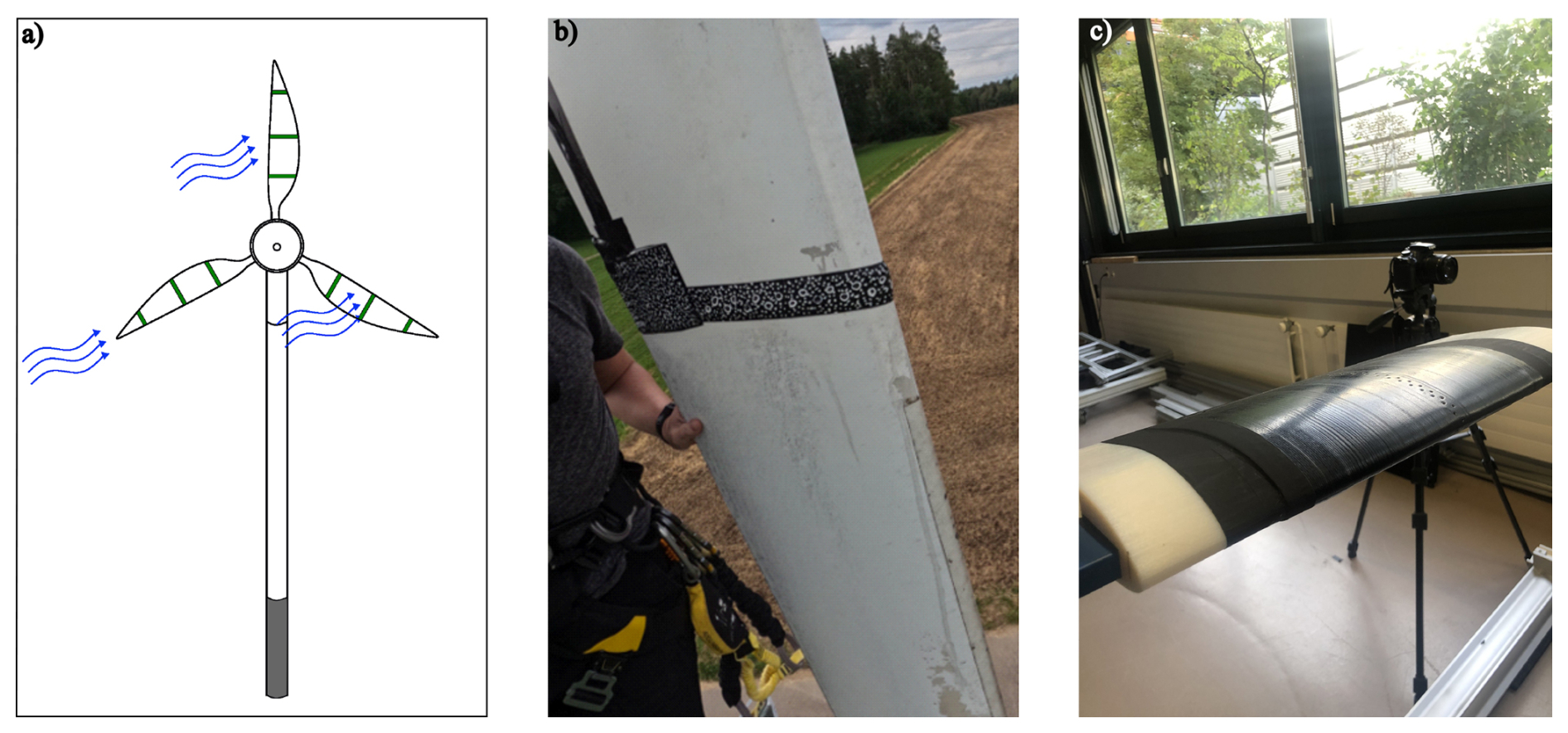
Figure 1(a) Intended use of Aerosense sensing units (green stripes) on a wind turbine in a real-world monitoring scenario, designed after Barber et al. (2022). (b) Aerosense system deployed on a wind turbine. (c) Close-up photo of the Aerosense sensing node (from the experiments conducted for this article).
Figure 1a schematically illustrates the intended deployment and use of the Aerosense system in a real-world monitoring scenario with several sensing nodes (green stripes) installed per blade. Figure 1b illustrates two Aerosense sensor nodes attached to a WTB.
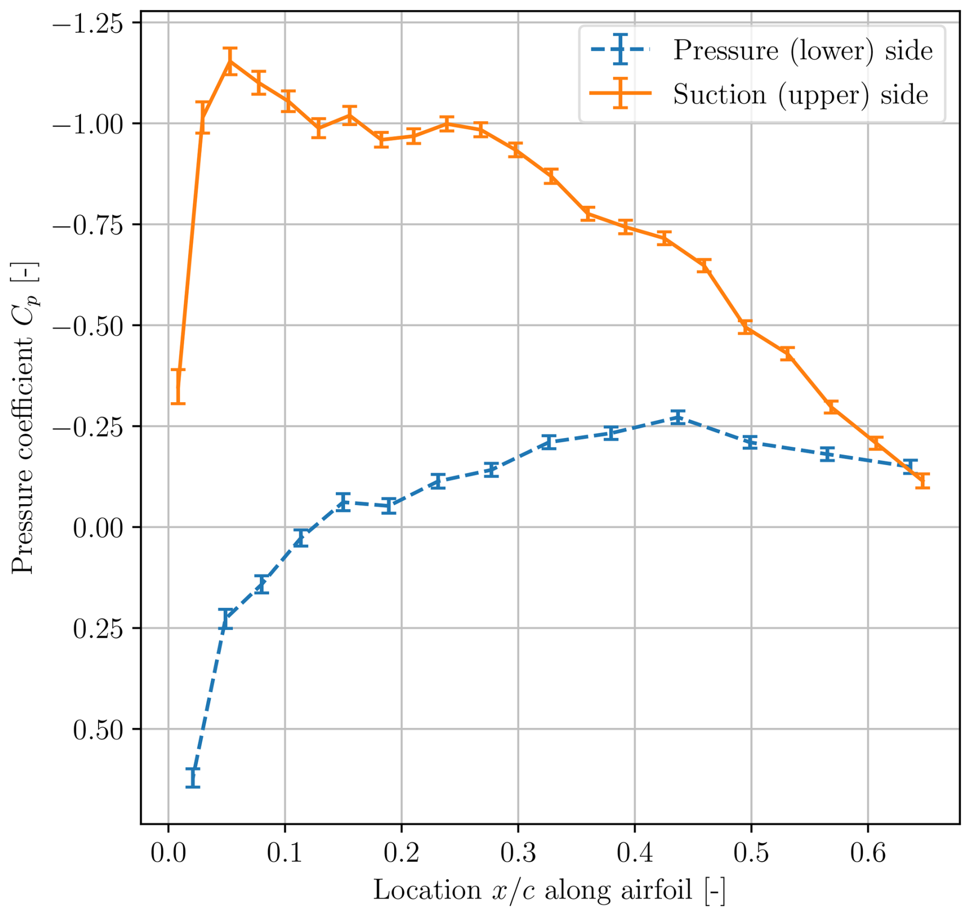
Figure 2Mean value of pressure distribution time series over NACA 633418 with an 8° angle of attack, a wind velocity of v=24 m s−1, an excitation frequency fh of 1.9 Hz, and a crack length of 0 % of the beam width. Error bars indicate the standard deviation. The pressure distribution was recorded using the Aerosense system in the experiments described in Sect. 3.
Figure 2 illustrates an exemplary pressure distribution recorded with the Aerosense system in the experiments described in Sect. 3. These recordings are transmitted via Bluetooth to the receiver base station, where the data are then fed to the software pipeline for supporting performance and condition assessment and digital twinning tasks. The Aerosense system was designed with the main aim of serving for inference of critical inflow quantities, such as the local angle of attack, and for the use in WTB leading edge erosion detection. The capacity to infer inflow conditions has been successfully tested and experimentally validated in wind tunnel experiments (Marykovskiy et al., 2023), which corroborated the accuracy and precision of the Aerosense system (Polonelli et al., 2022). To what concerns the latter aim, a method to detect and classify leading edge erosion has been designed based on synthetic data (Duthé et al., 2021; Barber et al., 2022). Although this system was not designed to serve the purpose of structural damage assessment, the premise of this work is that the indirect measurements offered by the Aerosense node can be leveraged to this end. With “structural condition assessment”, we refer to structural damage detection and the severity rating of the detected damage.
Only few instances in the existing literature attempt to derive structural damage by tracking aerodynamic quantities, with the majority of these efforts focused on aircraft and uncrewed aerial vehicles (UAVs). Among these efforts, Zhang et al. (2018) use dimensionless aerodynamic force and moment coefficients as inputs to a fuzzy logic system for fault detection on aircraft. The algorithm relies on the inference of aerodynamic force coefficients on the basis of acceleration measurements collected at different positions of the aircraft. Ruangwiset and Suwantragul (2008) utilize aerodynamic lift coefficients for the purpose of monitoring the structural health of UAVs in a wind tunnel study. The method relies on determining the lift coefficients based on acceleration measurements. As a common denominator of these works, vibration-based measurements are typically exploited, as these are more straightforwardly linked to damage. In this work, we wish to examine the indirect use of aerodynamic measurements, typically serving different purposes, for the task of structural condition assessment. Also related to our work, but not in relation to damage detection, are the following numerical and experimental studies focusing on the aerodynamic assessment of heaving airfoils. Veilleux (2014) performed numerical studies to analyze the influence of the plunging and pitching stiffness and damping on the oscillation of an aerodynamically loaded and elastically mounted airfoil, with the goal of optimizing fully passive flapping airfoil turbines. Ajalli et al. (2007) and Abdi et al. (2008) conducted wind tunnel studies with oscillating airfoils to experimentally investigate the influence of heaving and pitching amplitudes of the airfoil on the sectional aerodynamic pressure distribution around the airfoil. Finally, Madsen et al. (2022) developed the so-called “pressure belt” system, whose purpose and design are similar to the Aerosense solution. The pressure belt system is also packed in a thin sleeve, fixed non-intrusively to a WTB and aimed to measure the pressure distribution and inflow conditions on full-scale WTs. However, to our knowledge, the pressure belt system has not been used for damage detection so far.
As highlighted by the sparse literature, detecting structural damage on elastic, aerodynamically loaded structures like WTBs, based on the sectional aerodynamic pressure distribution around an airfoil, seems to be a novel approach. Consequently, we investigate in the present work for the first time whether structural damage, e.g., cracking, can be detected via the measured sectional aerodynamic pressure distribution over a 2D airfoil on an elastic, aerodynamically loaded, and vertically oscillating structure. For this purpose, we conduct a wind tunnel study where we record the aerodynamic pressure distribution over a heaving1 airfoil under various angles of attack, wind velocities, excitation frequencies, and structural states. Damage is introduced to the setup as a crack by gradually sawing the beam close to its support. Subsequently, we propose a multivariate algorithm based on convolutional neural networks (CNNs) to detect and rate the severity of structural damage.
The paper is structured as follows. In Sect. 2, we offer an overview of the adopted hypothesis and its theoretical foundations and associated limitations. Section 3 outlines the adopted experimental setup. The algorithm for damage detection and severity ranking, along with its basis, i.e., CNNs, is presented in Sect. 4. In Sect. 5, we describe the split of the experimental data and evaluate the proposed damage detection and severity ranking algorithm. Finally, in Sect. 6, we discuss the results obtained in the previous section based on the dynamics of the cantilever beam inferred from reference acceleration measurements and a finite element (FE) model. A summary of the main conclusions and directions for future research is offered in Sect. 7.
This work examines the hypothesis that aerodynamic pressure time series measurements can be exploited, when available, as indirect indicators of structural performance, thus serving the purpose of monitoring both aerodynamic performance and structural condition. This hypothesis is based on the argumentation that structural damage on an elastic structure, e.g., a crack or a delamination in a WTB, will induce a change in the stiffness (ΔKx) and damping (ΔDx) properties of the WTB. These changes alter the vibration of the elastic structure. Since the aerodynamic pressure distribution (see Fig. 2) depends on the interaction of the structure with the surrounding fluid flow, we expect the pressure distribution to be affected by a shift in the vibrational behavior of the blade. Hence, we postulate that changes in the aerodynamic pressure distribution, and correspondingly the normalized pressure coefficient, denoted by cp(x,c) (see Eq. 8), can be leveraged for structural damage assessment. However, the tracking of the evolution of the pressure distribution over time is non-trivial and typically requires an extensive measurement setup, involving intricate tubing (Traub and Cooper, 2008; Hu and Yang, 2008). We circumvent this issue by adopting the recently developed Aerosense system (Barber et al., 2022) to record the pressure distribution time series. This approach implicitly captures the variations Δcp(x,c) in the pressure distribution time series, providing an indirect indicator of structural damage. In support of this argumentation, we present a theoretical framework underpinning our hypothesis in Sect. 2.1 and refer to relevant experimental studies from the existing literature in Sect. 2.2. Subsequently, Sect. 2.3 and 2.4 describe an approach to testing the proposed hypothesis and elaborate on associated limitations.
2.1 Theory supporting hypothesis
The following set of simplified equations describes the dynamic instability of an airfoil, modeled as a single-degree-of-freedom (SDOF) system incorporating mass and damping, which is subjected to wind inflow and free heaving (see Fig. 3). Extensive theoretical exploration has been undertaken to understand the dynamic instability of this system in the context of galloping studies, e.g., in Blevins (1990) or in Modarres-Sadeghi (2021).
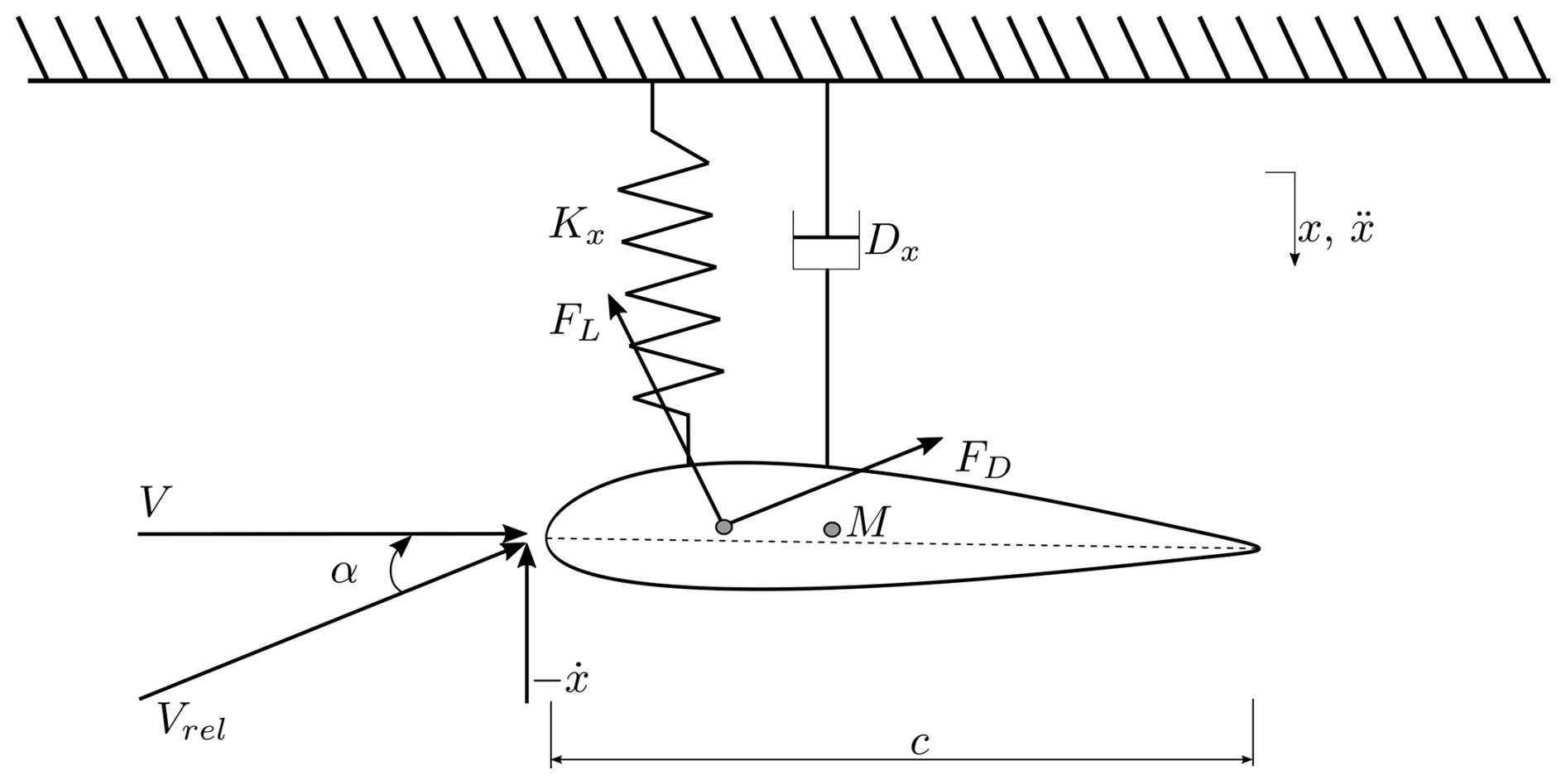
Figure 3Simplified schematic of a rigid, elastically mounted airfoil with symbolic representation of key parameters. The mass of the airfoil is denoted by M, the structural damping is denoted by Dx, and the spring stiffness is denoted by Kx. The displacement of the airfoil is described by x, the velocity is described by , and the acceleration is described by . The wind velocity is denoted by V, and the relative wind velocity is denoted by Vrel. The angle of attack is described by α, the aerodynamic lift force is described by FL, and the aerodynamic drag force is described by FD.
Equation (1) denotes the equation of motion of the SDOF system:
where M is the mass of the airfoil, while Dx denotes the structural damping and Kx denotes the stiffness in the x direction. The displacement, velocity, and acceleration of the SDOF airfoil model are denoted by x, , and . For Fx, the resulting vertical aerodynamic force acting on the airfoil, we assume
where ρ is the fluid density, c is the chord length of the airfoil section, V is the horizontal inflow velocity, and Cx is the total aerodynamic vertical force coefficient. Following Modarres-Sadeghi (2021), Fx can be expressed as a function of the angle of attack (AoA) α and the lift and drag coefficients CL and CD (Eqs. 3 and 4):
For small angles of attack, it follows that
Following Blevins (1990), employing a truncated Taylor expansion at α=0° to linearize Eq. (6) and reformulating Eq. (1) yields
From the right side of Eq. (7), it follows that a change in Kx, Dx or M, possibly caused by structural damage, not only affects the vibration of the airfoil, described by x, , and , but also alters its loading, the vertical aerodynamic force Fx. Since a change in Fx implies a change in the pressure distribution cp(x,c), we conclude that structural damage may indeed affect the pressure distribution around an oscillating airfoil and its variation Δcp(x,c). Although these equations indicate a relation between structural damage and the aerodynamic pressure distribution, one must keep in mind that these equations are simplified; a direct connection between damage and the pressure distribution is not established, as only integrated quantities are accounted for. Additionally, unsteady aerodynamic effects are not taken into consideration in these equations.
2.2 Experimental work supporting hypothesis
Our hypothesis is further supported by existing experimental studies. Ajalli et al. (2007) conducted experiments to investigate the aerodynamic pressure distribution of a heaving airfoil in conditions similar to those of our experimental campaign (see Sect. 3). These showed that increasing the heaving amplitude of the airfoil leads to amplified absolute values of the pressure coefficient cp and an amplified lag between the equivalent AoA αeq and the cp recorded close to the leading edge, which hints at an increased aerodynamic unsteadiness. Furthermore, Abdi et al. (2008) suggest that pitching motions with different rotational amplitudes also lead to pronounced changes in the maximal values of the cp close to the leading edge. As structural damage changes the modal properties of a structure and consequently its vibrations, these experiments support our hypothesis.
2.3 Testing of our hypothesis
The following considerations have led to the experimental setup that we propose in Sect. 3:
-
Rotatory-wing aerodynamics are more complex than fixed-wing aerodynamics. Since the aim of this study is to investigate whether it is at all possible to detect structural damage from aerodynamic pressure, we opt for a fixed-wing experiment. We approximate a fixed WTB by mounting an airfoil on an aluminum cantilever beam with a rectangular cross-section and placing it in a wind tunnel test section.
-
The flap-wise vibration of a rotating WTB is strongly affected by gravitational forces (Diken and Asiri, 2021). For that reason, we introduce periodic forcing at the tip of the beam to emulate the flap-wise vibration of a rotating WTB caused by the gravitational forces. Furthermore, we aim for a heaving amplitude of 5 to 10 cm at the mid-section of the airfoil, to obtain a non-stationary aerodynamic pressure distribution affected by the heaving, and choose both the tip mass and the excitation frequency accordingly.
-
To introduce structural damage, we decrease the cantilever's cross-section by sawing it close to its support. This reduction in the cross-section mimics the stiffness reduction caused by a crack. The crack length will be increased stepwise such that different structural states can be regarded. Within each state, the structure will be subjected to different combinations of AoA, wind loading, and tip excitation.
2.4 Scope and limitations of the chosen approach
2.4.1 Material and damage representation
An important limitation of our setup lies in the choice of material and the manner in which damage is introduced. While real-world WTBs are composed of layered composite materials exhibiting complex failure modes such as delamination and fiber breakage, our experiments employ an aluminum cantilever with damage emulated via saw cuts. This simplification allows controlled, repeatable tests and the ability to systematically vary damage severity. Although the artificial crack does not fully replicate the morphology or fracture mechanics of a naturally occurring defect in composites, it produces a measurable stiffness reduction, which is central to our proof-of-concept study.
2.4.2 Inflow, excitation, and environmental conditions
Our investigation is conducted in a wind tunnel facility under controlled environmental and operational conditions (EOCs) which do not reflect the complexity of the EOCs of real-world wind turbines. However, given the indirect nature of aerodynamic pressure as a proxy for structural condition, a controlled environment is necessary to observe and isolate the underlying mechanisms governing damage detectability; thus this paper does not aim to answer whether it is possible to detect and rank the severity of structural damage under real operational (rotating wing aerodynamics, pitching, tension stiffening, etc.) and environmental (high turbulence, varying temperature and weather) conditions of a wind turbine, and its findings are not directly transferable to full-scale wind turbines. Instead, this paper rather aims to offer a proof of concept as to whether such highly indirect pressure measurements can be conceived for use within an SHM setting and to lay the groundwork for further research and the justification for scaled-up experimental campaigns under more realistic and variable EOCs.
Furthermore, the tasks of damage localization and classification in SHM are not examined herein, since the distribution of Aerosense patches along a blade, i.e., the aspect of sensor placement, is not investigated; instead, we focus on investigations at the airfoil level. Moreover, the periodic excitation employed in our experimental setup may pose a limit for damage identification, as the corresponding periodic vibration response is larger than the transient vibrations caused by the aerodynamic loading and thus could complicate the identification task. The purpose of this work is to instead offer a first indication as to whether aerodynamic pressure distribution time series of low turbulent aerodynamics may be used to detect and rank the severity of damage on elastic and aerodynamically loaded beam-like structures.
3.1 Experimental setup
The experimental setup (Fig. 4) consists of an airfoil mounted on a flexible cantilever beam, placed in an open test section of a wind tunnel of the Unsteady Flow Diagnostics Laboratory at the École Polytechnique Fédérale de Lausanne (EPFL). The test section measures approximately 40 cm × 40 cm, and the wind tunnel can operate with a maximum wind speed of approximately 35 m s−1. As presented in Fig. 4, the aluminum cantilever beam has a rectangular cross-section with a height of 1 cm and a width of 4 cm. The clamped support of the beam is realized via a screwed connection, which is fixed to an aluminum frame, as illustrated in Fig. 5a. The aluminum frame, acting as a support structure, is placed on polymer mats to reduce the influence of ambient vibrations. Close to the support, damage is induced by gradually sawing the beam, which locally reduces its stiffness. The damage severity is quantified by measuring the length of the introduced cut. Multiple “crack” lengths are tested: 0 %, 12.5 %, 25 %, 37.5 %, and 50 % of the overall beam width (see Fig. 5b). At the mid-span of the beam, the NACA 633418 airfoil with a chord length c=16 cm and a width of 45 cm is aligned with the test section of the wind tunnel. Two 3D-printed airfoils were designed with specific slot angles, where the beam passes through, allowing two AoAs to be tested, namely 0° and of 8°. As the cantilever beam gets damaged during the tests and changing the AoA would imply removing the airfoil and wide parts of the measurement equipment, we use two identical aluminum beams: one for experiments with 0° AoA and one for experiments with 8° AoA. At the tip of the aluminum beam, a motor, controlled by an analog power source, rotates an eccentric mass and thus applies a harmonic excitation, which induces flap-wise bending, as indicated by the red arrows in Fig. 5a. Torsional motions (purple arrow in Fig. 5a) might also appear under such an excitation but are secondary relative to the main bending of the blade. The Aerosense system records the sectional aerodynamic pressure distribution over the airfoil profile at the mid-section of the airfoil (see Fig. 4). Reference accelerometers are used to record the acceleration in the y direction at five different positions, as indicated via the orange dot annotation along the cantilever beam shown in Fig. 4. The cantilever with the airfoil and the harmonic loading is conceived as a proxy setup, whose purpose is to emulate a rotating WTB oscillating in its flap-wise direction due to gravitational loading.
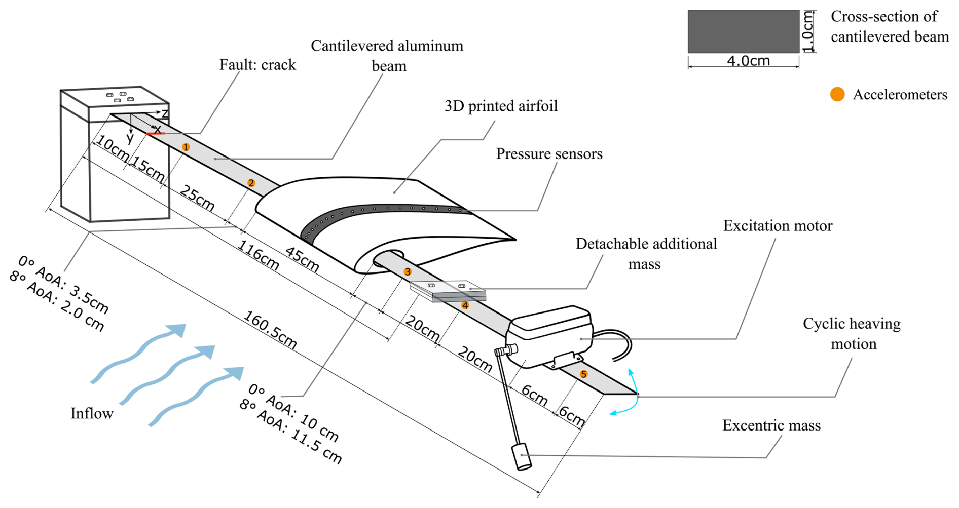
Figure 4The experimental setup at EPFL consists of a cantilever beam carrying an airfoil, an excitation motor, and a detachable additional mass, and it is positioned in the open test section of a wind tunnel. Measurement instrumentation is present on the airfoil in the form of the Aerosense system and on the cantilever beam in the form of accelerometers. The width and height of the rectangular cross-section of the beam are shown in the upper-right corner of the figure.
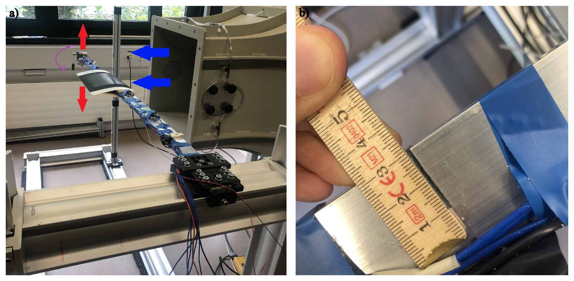
Figure 5(a) Experimental setup. The blue arrows indicate the direction of wind flow from the wind tunnel, the red arrows show the direction of oscillation of the cantilever beam, and the purple arrow points to the direction in which the beam twists. (b) An example of the sawed cantilever beam, where the crack length is 20 mm. View from above.
3.2 Measurement system
To record the aerodynamic pressure at the mid-section of the airfoil, we install the Aerosense sensing node, introduced in Sect. 1, at this position. The sensing node comprises 40 MEMS absolute pressure sensors sampled at 100 Hz, embedded in the previously described sleeve. In this experimental setup, the Aerosense system also has the advantage to be easily installed and reused for the two tested airfoils. Figure 2 shows the pressure distribution measured by the absolute pressure sensors after calibration. To compare pressure distributions from different inflow velocities, we compute the pressure coefficient cp(x,c) from the Aerosense data using the following expression:
where c denotes the chord length and p(x,c) denotes the pressure measured at the position (x,c) on the pressure or suction side of the airfoil. The pressure measured in the free stream is described by p∞, the density of air is described by ρ∞, and V∞ is the fluid velocity in the free stream. We compute p∞ based on the zeroing measurements conducted before and after every test block (explained in Sect. 3.3), and V∞ is set to the wind velocity of the corresponding experiment. Reference piezoelectric accelerometers are installed at five positions along the beam (see Fig. 4) and are connected via adhesive petro wax to the surface of the beam. They are positioned at the mid-section of the beam in the transverse direction, which is denoted as the z direction in Fig. 4. The acceleration signal is sampled at 2000 Hz.
3.3 Design of experiments
During the experiments, the aerodynamic pressure distribution time series at the location of the Aerosense sensing node is recorded for increasing damage severity, induced by the stepwise extended crack length, under various boundary conditions. Furthermore, we measure the acceleration acting on the beam at the locations of the accelerometers (see Fig. 4) in each experiment. To emulate different operational and environmental conditions, the experiments are conducted under two different AoAs: α1=0° and α2=8°. These two angles correspond to two conditions where the derivative of the aerodynamic force with respect to the AoA differs and alters the aerodynamic damping in Eq. 7. For each AoA, two different wind speeds (V1=12 m s−1, V2=24 m s−1) and two different excitation frequencies ( Hz, Hz) are considered. The Reynolds number is, respectively, and , and the reduced frequency k lies in the range of 0.021 to 0.08. The Reynolds number and reduced frequency were computed using the following expressions, where μ∞ denotes the free-stream kinematic viscosity of air and ρ∞ denotes the free-stream density of air:
where kg (ms)−1 and ρ∞=1.2250 kg m−3 (Anderson, 2017);
where ωM=2πfh in rad s−1 (Hodges and Pierce, 2011).
We use the standard values for μ∞ and ρ∞ at sea-level altitude and 15 °C, as these approximate the environmental conditions during the experiments. Two AoAs, two wind speeds, and two heaving frequencies result in eight test series (TSs) that are summarized in Table 1. For each test series, we consider five different crack lengths, along with one state with an added mass and a crack length of 0 mm. While the cuts with different lengths should represent the stiffness reduction in cracks of different length, the added mass is meant to represent ice accretion, also known as “icing”, on the WTB. Thus, there is a total of six structural states per test series (see Table 3). For each combination of structural state, AoA, wind velocity, and heaving frequency, we conduct three measurement runs (later also called “experiments”) of approximately 150 s. During the first 15 s, the airfoil is only aerodynamically loaded, and, for the remaining 135 s, aerodynamic and harmonic forces both act on the airfoil simultaneously. After each “test block” consisting of a set of three experiments, we conduct zeroing measurements and re-fasten the screws on the support structure to ensure that the structural boundary conditions remain identical for all experiments. As during the zeroing measurements the cantilever beam is only loaded by ambient vibrations, the acceleration recordings of these measurements will be used later for structural identification. Every measurement and experiment is identified by its unique number; an overview of the numbering of experiments is given in Tables A1 (harmonic and wind loading), A2 (only harmonic loading), and A4 (ambient loading), along with the file “design of experiments” in the Supplement. The same experimental numbering is applied for both AoAs.
In this section, we propose a method to detect and rank the severity of structural damage employing the experimentally acquired pressure distribution time series. Our suggested method is based on a machine learning approach which relies on the use of a CNN. In what follows, we therefore first offer a brief introduction to CNNs and then explain the details of our method.
4.1 Convolutional neural networks
CNNs are a subclass of artificial deep neural networks that have been successfully applied as supervised learning schemes across a broad variety of tasks, such as image classification, natural language processing, and time series classification (LeCun et al., 2015; Ismail Fawaz et al., 2019). A CNN comprises convolutional layers, pooling layers, and fully connected layers (LeCun et al., 2015), which are schematically shown in Fig. 6. Applying a convolutional layer on input data (see Fig. 6) essentially translates into applying multiple filters on the input data (LeCun et al., 2015). However, in contrast to normal filters, the weights of convolutional layers are not predefined but learnable. One or several convolutional layers are usually followed by a pooling layer. Pooling layers, like “local” or “global” “average” or “max” pooling, reduce the dimensions of the previously extracted convoluted feature maps by taking the average or maximum of a window with a certain size (local pooling) or of the whole feature map (global pooling) (Ismail Fawaz et al., 2019). The last, fully connected layer(s) of a CNN determine the probability distribution over the regarded classes for the output of the preceding pooling layer (Ismail Fawaz et al., 2019). Thus, this last layer classifies the features, which were extracted beforehand by the convolutional layers and condensed by the pooling layers. While the activation function “ReLU” is often used in convolutional layers, the activation function “softmax” is used in the last layer for multi-class classification. During the training phase in a supervised learning scheme, the filter values (weights and biases) of the convolutional layers are optimized through backpropagation. Thus, convolutional layers learn to extract discriminative features (Ismail Fawaz et al., 2019).
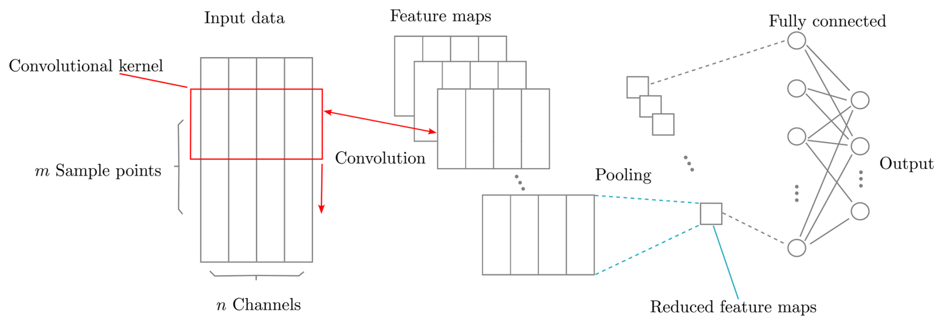
Figure 6Simplified schematics of a CNN architecture that takes multivariate time series windows with a length of m sample points and n channels as input. A 1D convolution is carried out by “sliding” a convolutional kernel vertically over the time series data. The feature maps resulting from convolution with different kernels are condensed by a pooling layer. The classification of the compressed feature maps, coming from the pooling layers, takes place in the fully connected layers at the end of the network.
4.2 Proposed damage detection and severity ranking algorithm
The proposed damage detection and severity rating algorithm is based on the CNN architecture proposed by Wang et al. (2017). This architecture, shown in Fig. 7, consists of three convolutional layers, where each one is followed by a batch normalization layer and activated with the ReLU activation function, a global average pooling (GAP) layer, and a final, fully connected layer using the softmax activation function. Our input data consist of multivariate time series samples. On these time series samples, the first convolutional layer applies 128 kernels with a length of 8, the second one applies 256 kernels with a length of 5, and the third one applies 128 kernels with a length of 3. All convolutional layers use zero padding and a stride of 1 and are followed by batch normalization layers to accelerate the convergence and to improve the generalization of the network (Wang et al., 2017). Subsequently, in the GAP layer, the feature maps coming from the third convolutional layer are strongly reduced and classified by the final, fully connected layer.
We decided to adopt a CNN-based architecture instead of a more sophisticated network architecture, such as recurrent or attention-based neural networks that were also successfully employed for time series classification (Ismail Fawaz et al., 2019; Mohammadi Foumani et al., 2024). Our decision is motivated by the fact that the number of trainable parameters in the proposed CNN architecture – 302 342 parameters – is substantially lower than in the abovementioned alternative architectures, which typically involve significantly more complex networks. As the size of our experimental dataset is small, we expect a CNN to better generalize due to fewer learnable parameters and expect the more sophisticated architectures to overfit on our training dataset.
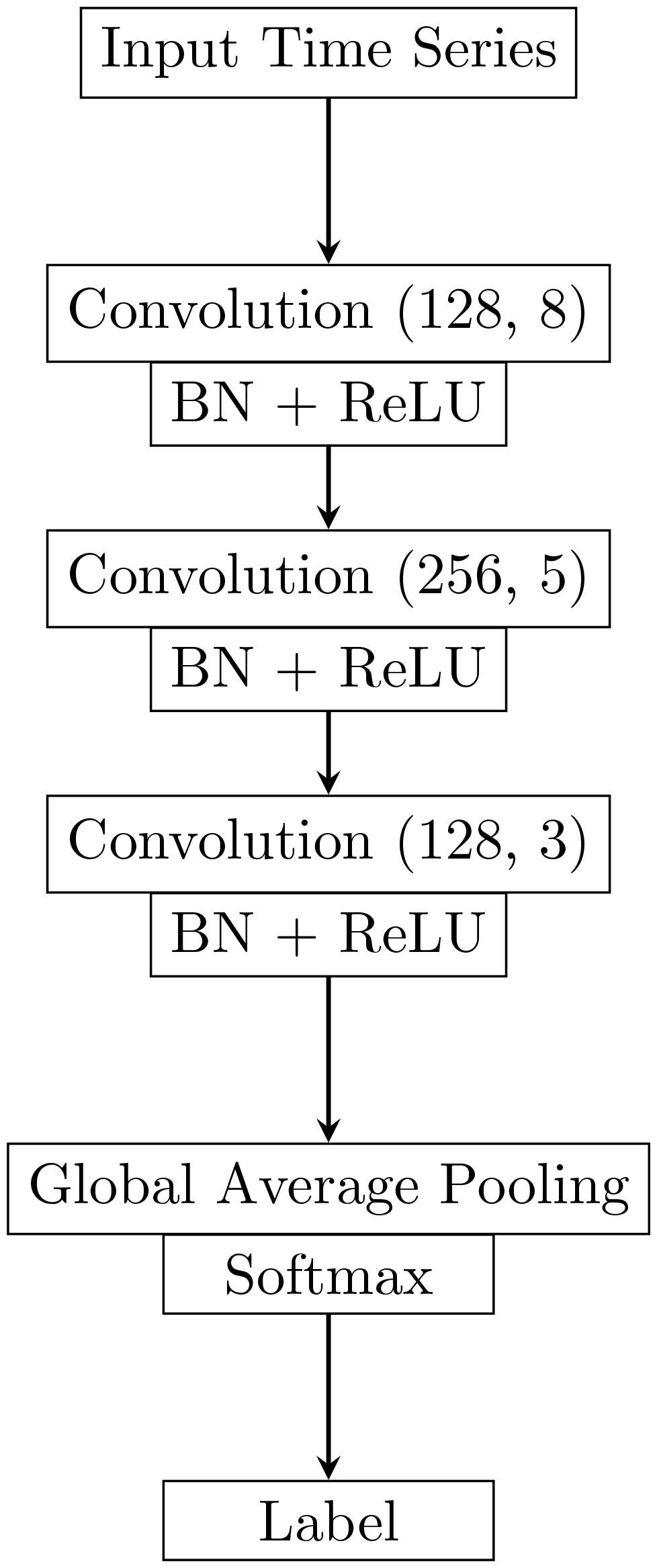
Figure 7CNN architecture for time series classification proposed by Wang et al. (2017) consisting of three convolutional layers with batch normalization and rectified linear unit activation functions (BN + ReLU) and a GAP layer with a softmax activation function. The convolution layers have either 128 or 256 kernels with a size of 8, 5, or 3 – as indicated by the number in the respective field. The figure is based on Fig. 1 of Wang et al. (2017).
We initialize the weights and biases of the network using Glorot's uniform initialization scheme (Glorot and Bengio, 2010) with a fixed random seed and employ the Adam algorithm (Kingma and Ba, 2015) to optimize the network weights and biases to minimize the loss function (sparse categorical cross-entropy loss). Following Ismail Fawaz et al. (2019), we use a model checkpoint procedure on the validation set, meaning that the model that performs the best on the validation set during the training process is used for the final evaluation. Furthermore, we use a batch size of 10 multivariate time series samples, and we initiate the training process with a learning rate of 0.05 that we reduce by a factor of 0.5 once the validation loss of the model does not improve for 15 epochs. The learning rate reduction is also done according to Ismail Fawaz et al. (2019); however, as we train our CNN for 150 epochs only, we increase the starting value of the learning rate to 0.05 and decrease the number of epochs required for an update of the learning rate from 50 to 15 to accelerate the optimization of the network weights. Apart from that, we do not modify any hyperparameters of the CNN proposed by Wang et al. (2017).
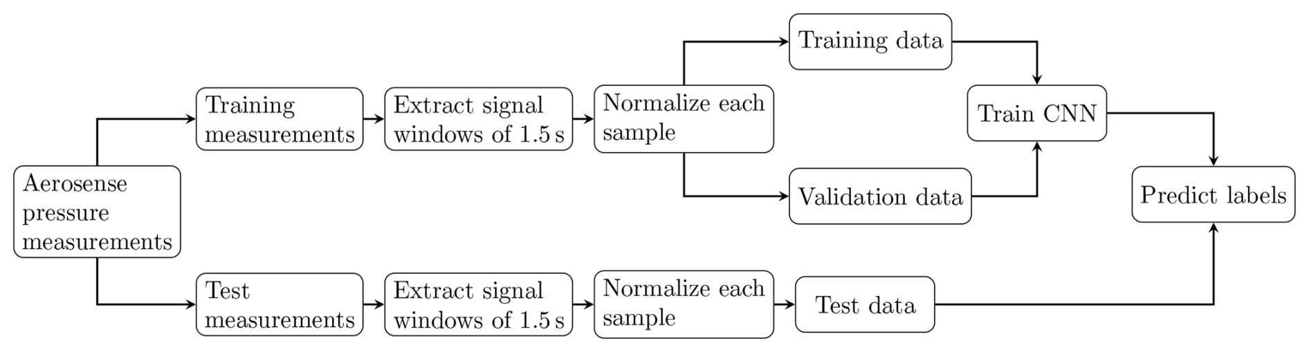
The input to the neural network consists of multivariate time series windows with a length of 1.5 s. Figure 9 illustrates in panel (a) an extract of 15 s length of the raw signal recorded by sensor 14 (located at on the suction side of the airfoil) of the Aerosense system under 0° AoA, V=12 m s−1, and fh=1.0 Hz (experiment 3; see Table A1). In the spectrogram in panel (b) of Fig. 9 and in the power spectral density (PSD) in panel (c) of the same figure, one can see that the maximum power of the signal is concentrated around approximately 1.95 Hz and that this is also the only distinctive peak in the signal. This also applies beyond 16 Hz. We also observe the peak at ≈ 1.95 Hz and the absence of further distinctive peaks for the other sensors and for measurements conducted with 8° AoA (see Fig. A1). The spectrogram in panel (b) is based on a discrete short-term Fourier transformation, conducted with SciPy (Virtanen et al., 2020). The PSD in panel (c) is computed using Welch's method and its implementation in SciPy (Virtanen et al., 2020). Both the spectrogram and the PSD use the raw pressure time series recorded by sensor 14 in experiment 3 with 0° AoA. The peak in the PSD at approximately 1.95 Hz closely coincides with the eigenfrequency of the first flap-wise eigenmode of the cantilever beam (see Table A4). Therefore, we choose signal windows of 1.5 s length as input for the CNN, such that each time window contains approximately three periods of pressure variations related to the vibration of the cantilever beam. As one can further see in the spectrogram shown in spectrogram in panel (b) of Figs. 9 and A1, there are low-frequency disturbances present in the frequency band between 0–0.8 Hz. These disturbances are most likely caused by sensor drift. By employing signal windows with 1.5 s length as input data, we also seek to limit the influence of these disturbances on the classification results. After extracting these signal windows from the raw pressure time series, we normalize each multivariate signal window by deducting the mean of the window and dividing it by the overall standard deviation of the signal window. Together with splitting the experimental data into a training, validation, and test set, this leads to the damage detection and ranking algorithm presented in Fig. 8.
We chose to only minimally tune the algorithmic hyperparameters, as we would like to show that structural damage assessment based on aerodynamic pressure measurements can be achieved with a generic ML scheme, without necessitating much effort. It is not our goal to achieve an optimized classification accuracy on such a small dataset, since this might not generalize well beyond our experimental setup. Rather, we aim to ensure that replication of our results may be easily achieved. For our implementation, we employed Keras 2.14.0 (Chollet et al., 2015) with the TensorFlow 2.14.0 (Abadi et al., 2015) back end.
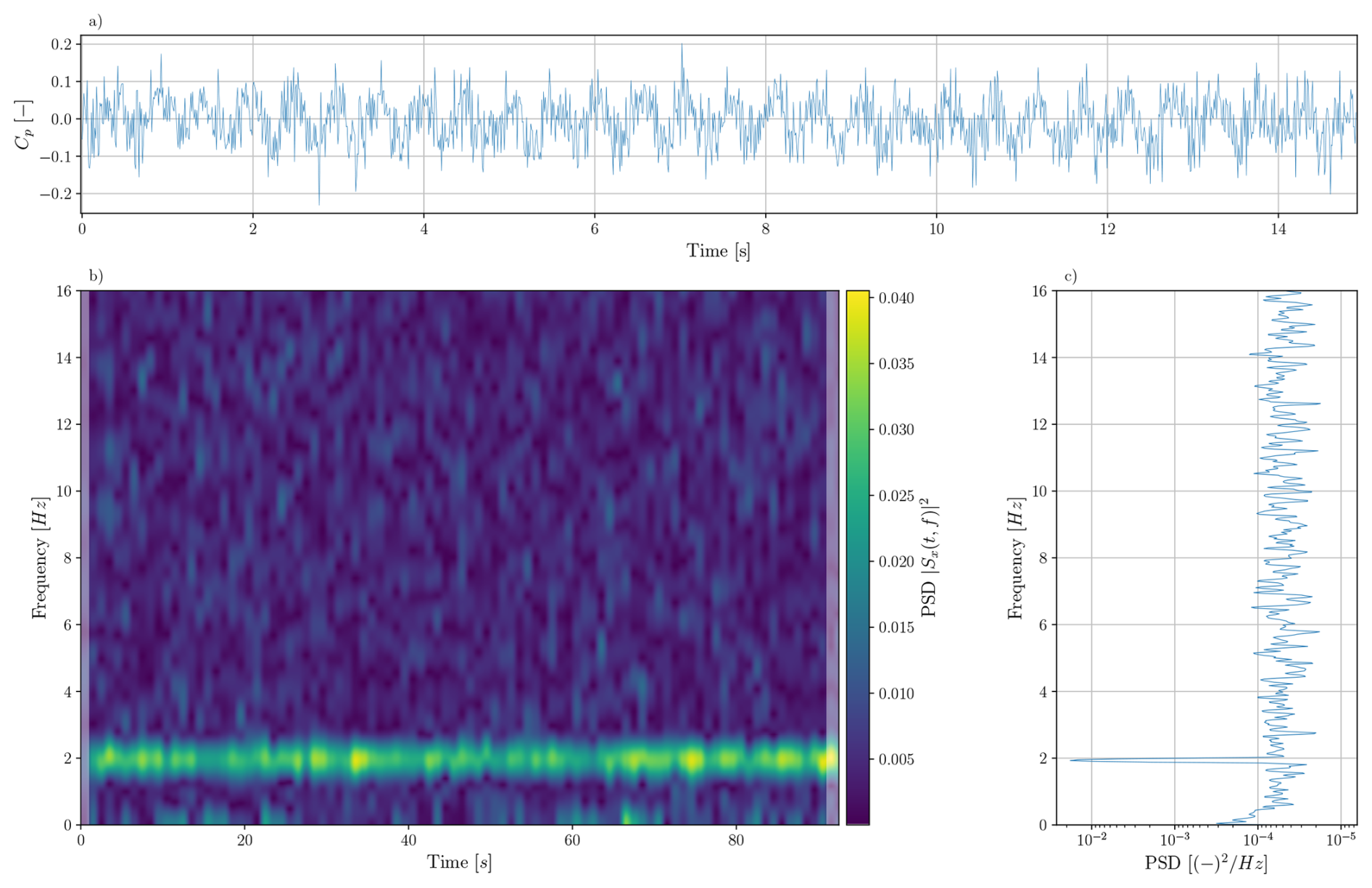
Figure 9(a) Extract of the pressure time history recorded by sensor 14, located at on the suction side of the airfoil, with 0° AoA under V=12 m s−1 and fh=1.0 Hz in experiment 3. Panel (b) shows how the spectrum of the pressure time history of sensor 14 of experiment 3 with 0° AoA varies over the whole duration of the experiment via a spectrogram. The spectrogram is computed using the discrete short-term Fourier transformation of SciPy (Virtanen et al., 2020). The shaded areas at the left and right ends of the spectrum indicate areas affected by sliding windows that are partially outside of the analyzed signal. Panel (c) depicts the PSD of the same signal computed over the whole duration of experiment 3 and is calculated with Welch's method and its implementation in SciPy (Virtanen et al., 2020).
This section first explains how the experimental data is divided into training and test datasets. Then, the accuracy of the proposed method for damage detection and severity classification is evaluated on these training and test datasets.
5.1 Split of the experimental data
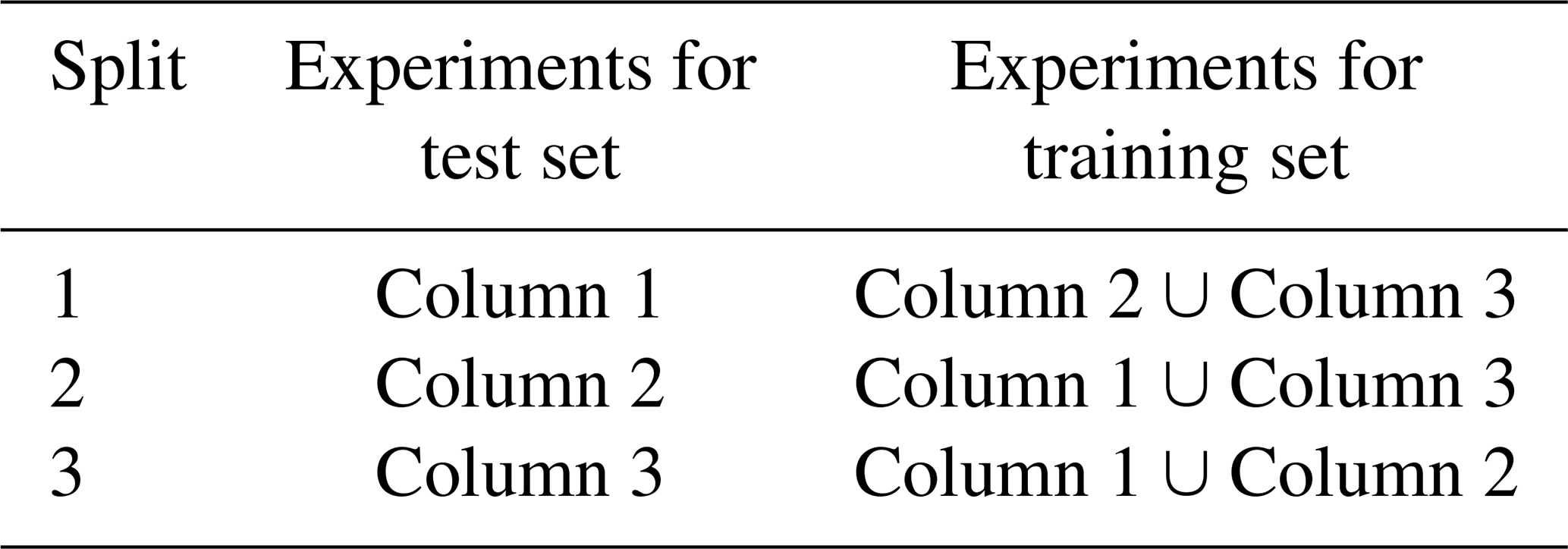
For detecting and ranking structural damage in the acquired experimental data with the method proposed in Sect. 4, we create two datasets, one that contains all measurements with 0° AoA and one with 8° AoA, as the pressure distribution strongly depends on the AoA. As described in Sect. 3.3, for every combination of inflow conditions and structural states, we record three sequential measurements of approximately 150 s duration. As we regarded two heaving frequencies fh, two wind velocities V, and six structural states, 72 multivariate pressure time series measurements are available in total per AoA. The three measurements of each combination of inflow conditions and structural states are not randomly divided into the basis for the training and test set; instead, a certain “split” always uses the same two measurements of the three available measurements of every combination of boundary conditions to generate training data, reserving the remaining measurement to generate test data. Thus we can evaluate the performance of our method on completely unseen data. Table A1 in the Appendix gives an overview of the boundary conditions of each experiment. Referring to the columns of Table A1, Table 2 describes the composition of the three splits.
Table 2Composition of the splits used to create the training and test sets to evaluate the multivariate algorithm. The “columns” refer to columns 1, 2, and 3 of Table A1.
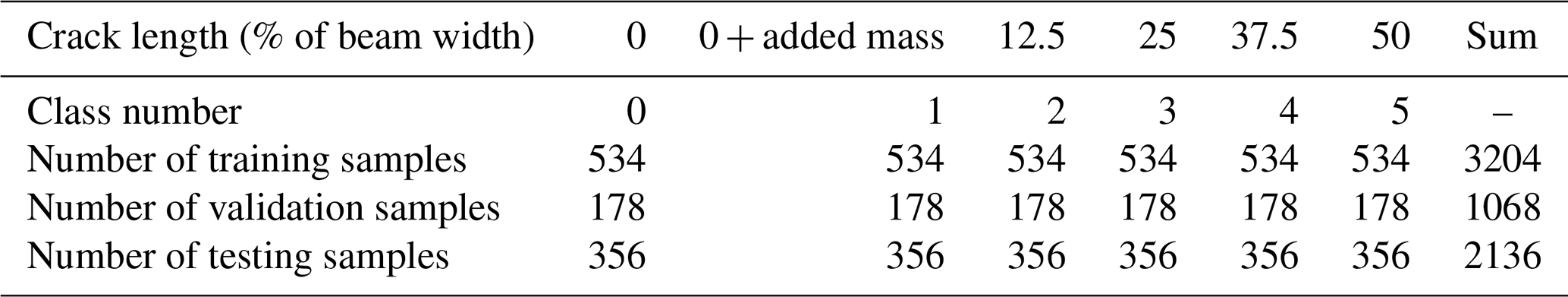
Consequently, we employ 48 experiments to generate the training samples and 24 experiments for the test samples. From each experiment, we neglect the first 40 s and the last 10 s to reduce the influence of transients from switching on the harmonic excitation and from possibly switching off the harmonic excitation too early. From the remaining approximately 100 s, we extract 89 multivariate signal windows of 1.5 s with an overlap of approximately 30 %. As a result, there are 4272 samples available for training and 2136 samples available for testing (see Table 3). Finally, 25 % of the training samples are reserved for validation purposes, and only the remaining 75 % of the training samples are de facto used for training the CNN. Thus, per damage class, there are 534 samples available for training, 178 samples for validation, and 356 samples for testing, as presented in Table 3.
Table 3Available samples for training, validation, and testing per class.
5.2 Accuracy of damage detection and severity ranking based on aerodynamic pressure measurements
The results of the proposed multivariate damage detection and severity ranking algorithm are subsequently presented via confusion matrices in Fig. 10. In our experiments, we consider structural states with a crack length of 0 %, 12.5 %, 25 %, 37.5 %, and 50 % of the beam width, along with one state with 0 % crack length and an additional mass of 246 g attached to the beam (see Table 3). The mapping of the structural states to the class numbers can be found in the first row of Table 3.
Figure 10a depicts the classification results for split 2 of the dataset with 0° AoA, and Fig. 10b depicts them for 8° AoA.
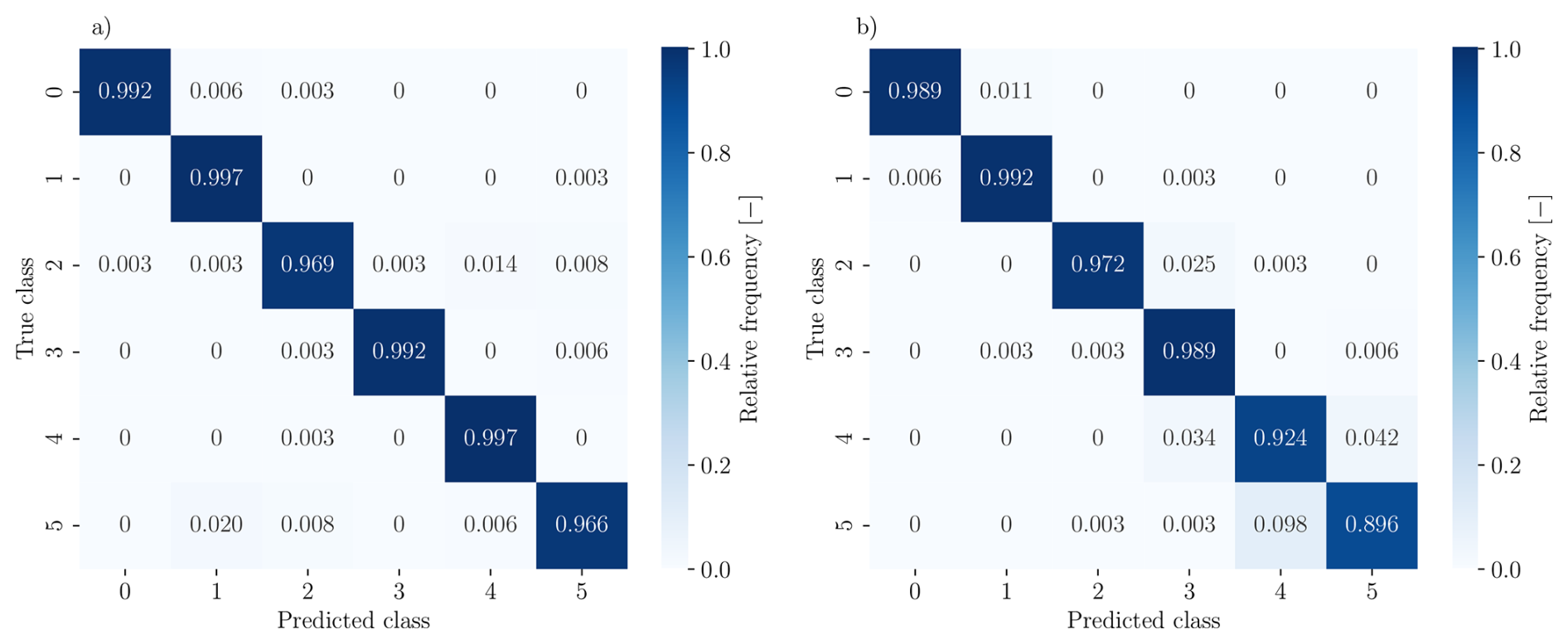
Figure 10Classification results for split 2 of both datasets depicted by confusion matrices and rounded to three decimal places for non-zero values. The rows correspond to the true class of a sample; the columns correspond to the class predicted by the proposed method. The relative frequencies are rounded to three decimal places. Panel (a) shows the results for 0° AoA, and panel (b) shows the results for 8° AoA.
For the data with 0° AoA, the classification of the aerodynamic pressure times series samples works very reliably. Only two samples from a damaged state are classified as undamaged, and these even stem from the state with the smallest damage (see Fig. 10a). For 8° AoA, the classification also works well, but 12 % of the samples of damage class 5 are falsely classified as damage class 4 (see Fig. 10b). However, these two classes are neighboring, and the detection of damage from any of these two states would require an immediate response. Figure 10 shows the classification accuracy of the best-performing split. In Table 4, we present the classification accuracy averaged over all balanced classes for all regarded splits.
Table 4Accuracy for all splits for 0 and 8° AoA. The classification accuracy given for a single split is the average of the classification accuracy over the six balanced classes of that split.
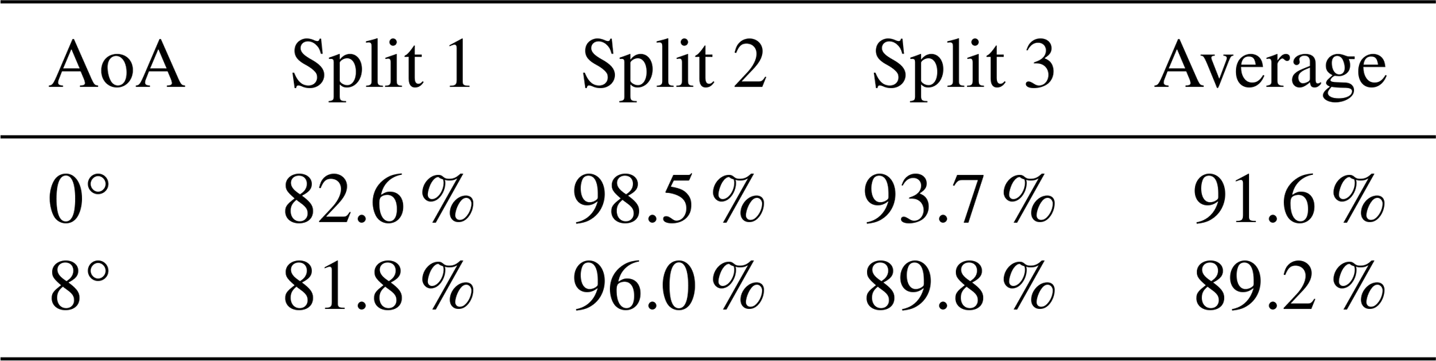
The overall slightly lower classification accuracy for 8° AoA and the corresponding more diffuse confusion matrices are likely to be related to the more turbulent, unsteady aerodynamics which typically emerge due to more detached flows at higher angles of attack.
Furthermore, we observe a consistent confusion between damage classes 4 and 5 at 8° AoA in Fig. 10. In the set of considered damage states, the variation from class 4 to 5 represents the smallest relative change between two damage states and, following Fig. 11, particularly the acceleration amplitudes and thus also the velocity amplitudes for experimental series 5 and 6 (corresponding to damage classes 4 and 5) are highly similar at 8° AoA. Based on the simplified relationship of Eq. (7), this indicates similar pressure distributions. This, in combination with only minor shifts in the structural eigenfrequencies (see Sect. 6.2) between these two damage states, likely contributes to significant overlap in the learned feature representations. Moreover, the increased aerodynamic unsteadiness and turbulence at higher AoA further reduces the signal-to-noise ratio, making it more difficult for the model to distinguish subtle structural differences. Given these factors, and considering the limited capacity of the small CNN architecture used in this study, the observed confusion is not unexpected.
Another remarkable point is the systematically lower classification accuracy for first split of both datasets. We hypothesize that the systematically lower classification accuracy for the first split (see column 1 of Table 4) is caused by uncaptured transients in the wind flow resulting from wind tunnel activation, as the wind tunnel was the only device in the experimental setup running all the time during the three subsequent experiments conducted for each combination of boundary conditions. This is a point that must be investigated and improved in future experiments. However, as the averaged classification accuracy lies for both datasets at 91.6 % and 89.2 %, respectively (compare Table 4), and the lower bound of all classification results is at 80.0 %, our experiments confirm our hypothesis that structural damage can be consistently detected and ranked based on aerodynamic pressure measurements in mildly turbulent environments. Considering further that the experimental data comprise different Reynolds regimes and excitation frequencies, these results indicate that the proposed damage detection and ranking pipeline based on an indirect sensing scheme is robust towards moderate variability in the environmental and operational conditions and is suited for damage detection on elastic, beam-like structures in mildly turbulent environments and warrants further investigation. Since our proposed time series classification method is purely data-driven, we cannot provide more extensive reasoning for how varying the AoA affects detectability. From a computational perspective, our algorithm is efficient: while the model is trained in approximately 445 s on a cluster node using an Intel Xeon Gold 6336Y CPU and a NVIDIA HGX A100 80 GB GPU, the test set is classified in approximately 1.8 s. This demonstrates that our proposed machine learning pipeline is well suited for structural health monitoring in the scope of real-time digital twin applications. Although the supervised learning approach employed in this study is not directly applicable to real-world scenarios due to the absence of labeled data, it serves as a first step to assess the viability of indirect aerodynamic pressure measurements for damage detection. The CNN architecture developed here may also provide a suitable encoder for future unsupervised anomaly detection approaches. Moreover, CNNs can easily be parallelized on GPUs or other ML-specific hardware, which may potentially allow fast on-the-edge damage detection for WTBs when integrated with a system like the Aerosense node.
In this section, we use the reference acceleration measurements (see Sect. 3.3) to investigate the intricacy of the damage detection and classification task we attempt to solve with our proposed approach, as introduced in Sect. 4. Using the hypothesis of Sect. 2, the preceding section discusses how to adopt a CNN-based scheme to detect structural damage from aerodynamic pressure measurements in a supervised manner. An alternative approach to damage detection would be to rely on vibration-based information. By analyzing the measurements of the installed acceleration sensors, we can more targetedly investigate the dynamic behavior of the system that was previously only indirectly observed via the aerodynamic pressure measurements. For that purpose, we analyze subsequently how the amplitudes of the acceleration signal at the tip of the cantilever beam and the eigenfrequencies fi of excited eigenmodes ϕi develop with increasing crack length. Finally, we also discuss the influence of the orientation of the crack on the dynamics of the cantilever beam using a FE model of the cantilever beam.
6.1 Evolution of the vibration amplitudes with increasing damage
The choice of examining the acceleration amplitude as a proxy to damage is motivated by two facts: firstly, the cantilever beam in the experimental setup is expected to vibrate in a quasi-steady state after initial transients have been damped out, under the influence of the periodic forces FΩ caused by the rotating mass and the aerodynamic loading Faero. We assume here that the system oscillates in a quasi-steady state, since FΩ and the lift and drag forces of the airfoil vary periodically and the motion of the blade may additionally induce small vertical, transient loads caused by vortex shedding. As a result of the quasi-steady vibration state, a reduction in the beam stiffness is expected to lead to amplified vibration amplitudes under the prescribed loading. The more usual features to detect damage based on output-only acceleration data, such as eigenfrequencies, may be non-trivial to determine under forced conditions (when the input force is not measured). Secondly, the choice of analyzing the evolution of the acceleration amplitude is motivated by its linkage to pressure. Based on Eq. (7), the velocity and thus also the displacement x(t) and acceleration of the airfoil serve as inputs to the aerodynamic pressure distribution and its variation. To better understand the variation in the pressure distribution, we subsequently analyze the evolution of its inputs that are related to the dynamics of the cantilever beam by examining the acceleration amplitude with growing damage. Since the beam vibrates in a quasi-steady state, the evolution of the displacement and velocity amplitudes with increasing damage can be approximately inferred from the evolution of acceleration amplitudes. To analyze the evolution of the acceleration amplitudes with increasing damage, we compute the root-mean-square (RMS) value of the acceleration time histories, as this feature characterizes the average amplitude of a noisy signal. The RMS of a discrete time signal yk with k ϵ is computed as . For computing the RMS, we neglect the first 40 s and the last 10 s of each acceleration signal to limit the influence of initial transients or shutting down the rotational motor too early.
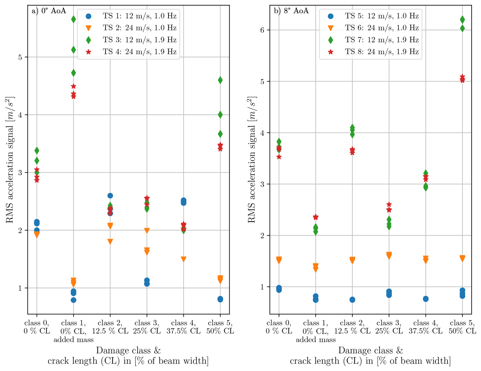
Figure 11RMS values of the acceleration signals recorded by accelerometer 5, located at the tip of the cantilever beam, for all test series (TS) and all damage classes. Each data point marks the RMS value of a single acceleration measurement. The color and marker of each data point indicate the corresponding TS and thus the approximate loading conditions. Panel (a) shows the RMS values of experiments conducted with 0° AoA. Panel (b) displays the RMS of acceleration measurements recorded with 8° AoA. Since three measurements were conducted for each combination of inflow conditions and structural state, three circles are visible per TS/damage class combination.
Figure 11a and b report the RMS of the accelerations measured with sensor 5 at the tip of the cantilever beam for all TS and every damage class. Every data point marks the RMS value of an acceleration signal in a single experiment conducted under the rotor, FΩ, and aerodynamic, Faero, loads. The RMS value is computed as previously described. In panel (a), we observe the RMS recorded for 0° AoA, while, in panel (b), results are reported for 8° AoA. The color of the data points refers to the TS of the measurement and indicates the loading conditions of the system during the measurement. Looking at the evolution of the RMS for a fixed set of loading conditions over different damage classes, e.g., TS 1 in panel (a), it is observed that, despite a growing crack and thus an increasingly reduced stiffness of the cantilever beam, the recorded acceleration amplitudes do not increase monotonically. Figure 11 does not reveal a strictly monotonic increase in acceleration RMS values with increasing crack length in all TS. We hypothesize that the non-monotonic trends result from the complex loading conditions and the orientation of the introduced crack, and we investigate this further in the subsequent sections. Furthermore, the vibration amplitudes that occur for different damage classes often overlap. This holds true, for instance, for the vibration amplitudes observed at crack lengths corresponding to 12.5 % and 25 % of the beam width for both examined AoAs. This implies that the use of vibration-based measurements as damage proxies would not be straightforward in this case and further reveals that the classification task which we solve using the CNN-based scheme is a non-trivial one.
6.2 Evolution of the eigenfrequencies with increasing damage
As a further damage proxy, we conduct an approximate calculation of the modal frequencies (eigenfrequencies) of the beam under increasing damage. We already explained that this calculation is non-trivial under a forced excitation regime, since the OMA requirements are not fulfilled. OMA methods are output-only; that is, they only require response measurements (as is the case for the available measurements here) and require that the examined structure be subjected to loadings with white-noise or at least broad-band characteristics that excite all mode shapes of interest (Brincker and Ventura, 2015). Therefore, we opt to use the acceleration measurements of all five accelerometers from the zeroing runs (see Sect. 3.3), where only ambient loading was present on the cantilever beam to conduct the modal analysis. We use automated frequency domain decomposition (AFDD), introduced by Cheynet et al. (2017), and its implementation in MATLAB (2021). AFDD is based on frequency domain decomposition that was originally introduced by Brincker et al. (2000, 2001a, b). The acceleration measurements collected under ambient excitation have an approximate length of 60 s. We discard the first 20 s of each acceleration measurement and extract signal windows of 10 s duration from the remaining signal, using a sliding increment of 0.5 s. Subsequently, the signal windows are preprocessed with a low-pass filter with a cut-off frequency of 100 Hz. In an additional step, we employ k-means clustering, introduced by Lloyd (1982), to group the previously identified natural frequencies and mode shapes into distinct clusters that represent different vibration modes of the analyzed structure. By computing the mean value μf,i and the standard deviation σf,i of each cluster i of natural frequencies, we obtain the uncertainty associated with the respective natural frequency. We use the same approach to compute the mean values and standard deviations of the relative displacements of each mode shape ϕi at the location of the sensors, thereby assessing the uncertainty related to the identified mode shapes. Finally, we refine the determined frequency clusters to identify reliable modes by eliminating natural frequencies that exceed a 5 % deviation from the respective cluster mean or are only detected in a small number of signal windows. The associated mode shapes are removed accordingly. Since the accelerometers installed on the beam can only measure accelerations along the y direction, we can only detect mode shapes which exhibit vertical oscillations. In the following, we only compute the eigenfrequencies and eigenmodes for the cantilever beam with the 0° AoA airfoil, as both employed cantilever beams are nearly identical (see Sect. 3).
The results of μf,i and σf,i for the eigenmodes up to 60 Hz in all structural states are given in Table A4. The evolution of these natural frequencies fi for increasing damage is presented graphically in Fig. 12. Additionally, the eigenmodes ϕi that have been identified for experiment 15 are exemplarily given in Fig. 13. While the mode shapes ϕ1, ϕ2, and ϕ5 are detected with low uncertainty in the data of experiment 15, the mode shapes related to f3 and f4 exhibit higher variance.
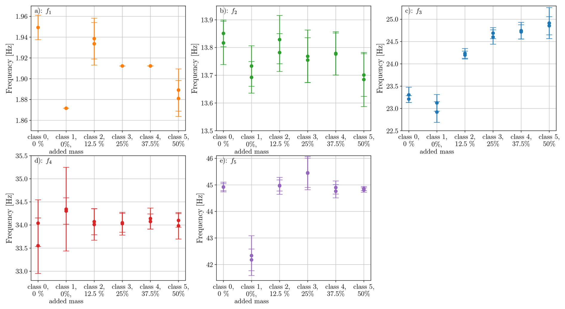
Figure 12Evolution of the mean values (circular markers) and standard deviations (error bars) of the first five eigenfrequencies fi, determined with AFDD and clustering, plotted over the damage classes. The exact values of fi for each damage class are given in Table A4. Eigenmode ϕ1 could not be detected in experiments 6 and 63, which correspond to damage classes 0 and 3; thus, for f1, there is only one value presented in damage classes 0 and 3.
In Fig. 12a and b the eigenfrequencies f1 and f2 of the first two vertically oscillating eigenmodes ϕ1 and ϕ2 exhibit an overall decreasing trend with increasing crack length (not considering damage class 1 with the added mass here). Considering the associated standard deviations of f1 and f2, this trend is more pronounced for f1. In contrast, the evolution of the eigenfrequencies f3, f4, and f5 is non-monotonic. Possibly, the eigenmodes corresponding to f3, f4, and f5 are sensitive towards perturbations in the boundary conditions of the system. Moreover, due to their higher variability, ϕ3 and ϕ4 might not represent merely vertically oscillating eigenmodes but coupled ones. To obtain further insight into the these eigenfrequencies and eigenmodes, we offer the results of a simulation in the next subsection, which aims to replicate the experiment. For the monotonically and approximately monotonically decreasing eigenfrequencies f1 and f2, it holds that the absolute change between the least damaged and the most damaged state is approximately 0.06 and 0.14 Hz, respectively. Based on the above, we deduce that the local stiffness reduction introduced by the crack only bears a limited effect on the eigenfrequencies of the identified eigenmodes, also rendering this an uncertain proxy for damage detection. We expect the orientation of the crack to contribute to variability in the estimated quantities, since the selected crack orientation is not chosen to reflect a pure bending crack but is rather a defect that allows large vertical oscillations under the chosen wind inflow conditions to affect the aerodynamic pressure distribution on the airfoil. We further investigate this effect based on the aforementioned simulation model.
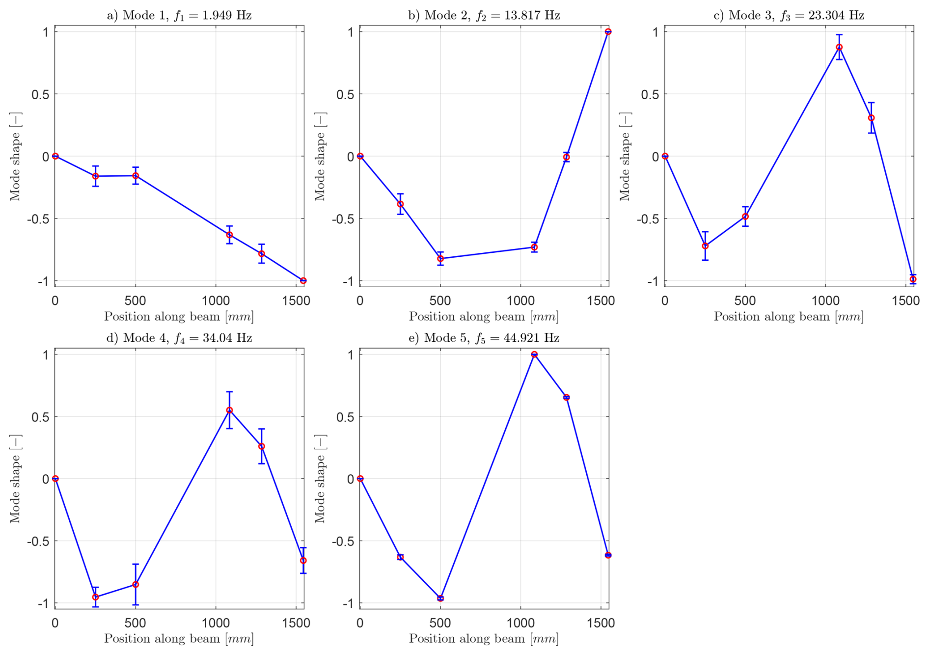
Figure 13Mode shapes of the first five vertically oscillating eigenmodes ϕi of experiment 15, determined with AFDD and k-means clustering. The error bars indicate the standard deviation associated with the relative vertical displacements of the degrees of freedom of each mode shape. The mode shapes are scaled to comprise a maximum value of 1.0.
6.3 Influence of the crack characteristics
In order to gain insights into the experimental configuration and some of the aforementioned observations, we have developed a FE model of the tested system and report on the estimated evolution of the acceleration amplitudes under constant loading and boundary conditions.
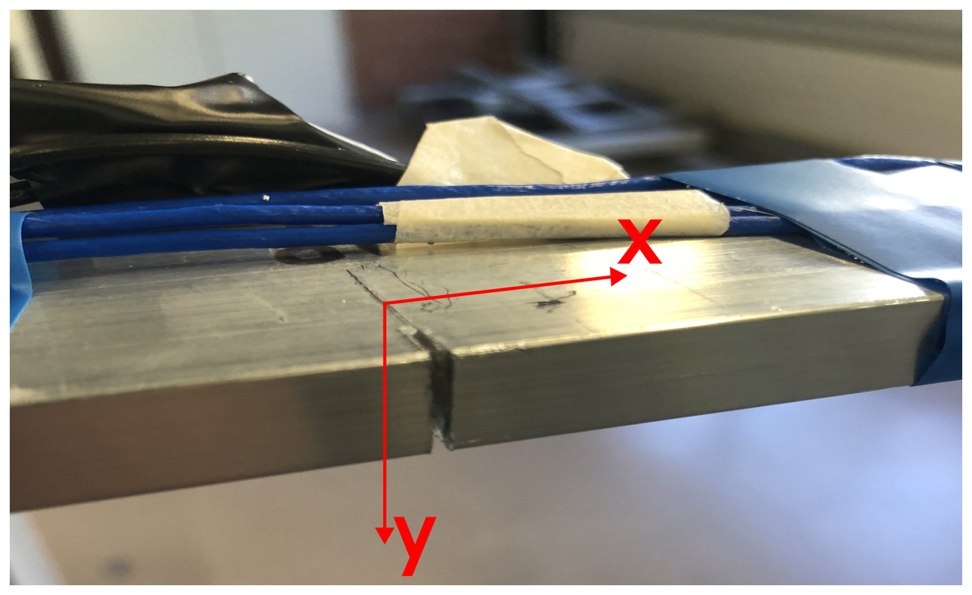
Figure 14Orientation of the actual crack present during the experiments. The rotational and aerodynamic loading lead to vibrations in the vertical (y) direction of the cantilever beam.
In our simulated analysis we neglect the aerodynamic force, Faero, since modeling the dynamic fluid–structure interaction occurring at the airfoil requires complex treatment, moving beyond the scope of simulating the essential dynamics of this system. The employed FE model, shown in Fig. 15a, is set up in the Abaqus 2022 finite element package and simulates the response of the cantilever beam under eccentric harmonic loading FΩ. The cantilever beam is modeled with 8-node general shear deformable shell elements with reduced integration (SR8 elements in Abaqus). Furthermore, a rigid beam section using B31 Timoshenko shear-flexible elements was added to the edge of the cantilever beam at the location of the rotating mass in order to account for the eccentricity of the periodic excitation. The displacement and rotation degrees of freedom at the left end of the beam are set to zero to model the rigid support of the cantilever (encastre boundary condition in Abaqus). The Young's modulus and density of the aluminum beam are set to 70 GPa and kg mm−3, respectively. The periodic resultant force FΩ acting on the cantilever can be expressed as a function of the rotating mass (mω), eccentricity radius (r), and excitation frequency (f): FΩ=mωr(2πf)2 and yields 0.777 N for an excitation frequency of Hz. The airfoil and the body of the excitation motor are modeled as lumped masses at the respective positions on the cantilever beam. As a consequence, the model neglects the additional stiffness introduced by the airfoil mounted on the cantilever beam in the experimental setup. The edge crack is introduced into the model as a seam object, resulting in a nodal discontinuity at the crack location with different lengths, ranging from 0 to 20 mm. To determine the first five eigenfrequencies fi,m and eigenmodes ϕi,m of the FE model, we conduct an eigenvalue analysis using the Lanczos eigensolver in Abaqus. The resulting eigenfrequencies fi,m and eigenmodes ϕi,m are shown in Fig. 15b and in the first row of Table A3. To compute the time-dependent response of the cantilever beam under harmonic loading, a dynamic (modal) analysis is carried out based on the results of the eigenvalue analysis. In such a dynamic (modal) analysis, the structural response of the cantilever beam under harmonic loading FΩ is determined for an excitation frequency fh=1.0 Hz for a period of 100 s and with a time increment of Δt=0.001 s. A modal damping ratio of 0.03, acting on the first mode, is considered. For each regarded crack length, such a simulation is conducted. Afterwards, the time history of the vertical acceleration at the location of sensor 5 (close to the tip of the beam, highlighted in Figs. 15 and 4) is extracted.
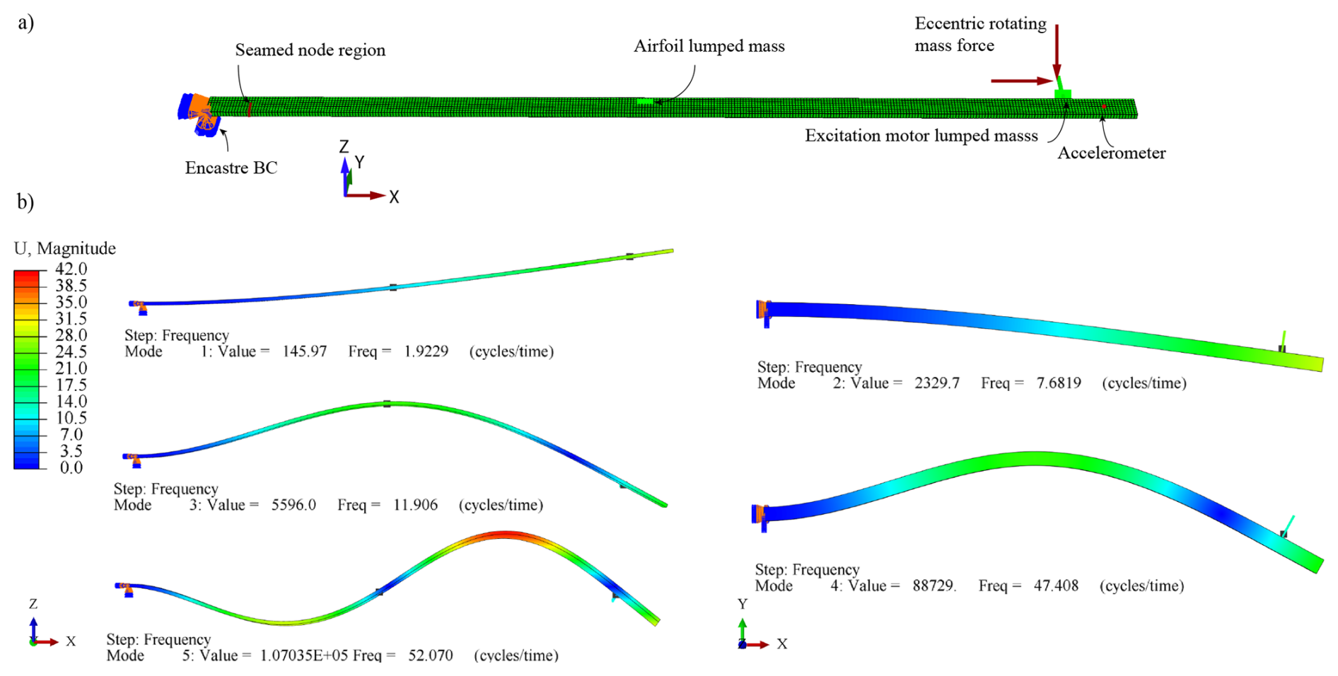
Figure 15(a) FE model of the cantilever beam. The presence of the airfoil and the excitation motor is reflected by the lumped masses. The vertical edge crack is introduced to the model as a seam object, resulting in a discontinuity with different lengths varying from 0 to 20 mm. The effects of the eccentric rotating mass are modeled as harmonic loading with eccentricity in the dynamic modal analysis. (b) First five mode shapes ϕi,m and corresponding eigenfrequencies fi,m and eigenvalues of the reference setup (undamaged beam).
The mode shapes ϕ2,m and ϕ4,m of the FE model oscillate only horizontally (see Fig. 15). As a consequence, these cannot be consistently identified with the experimental acceleration data and in the OMA, as the accelerometers along the cantilever beam only measure vertical accelerations. Comparing the experimentally determined mode shapes with the vertically oscillating mode shapes of the FE model, it is noticeable that the eigenvalue analysis of the FE model does not predict the modes ϕ3 and ϕ4 at 23.304 and 34.040 Hz.
Table 5Values of the modal assurance criterion (MAC) between the modes ϕi, determined by OMA, and the modes ϕi,m, computed from the FE model, rounded to two decimal digits. The most similar mode shapes are highlighted by a bold MAC value.
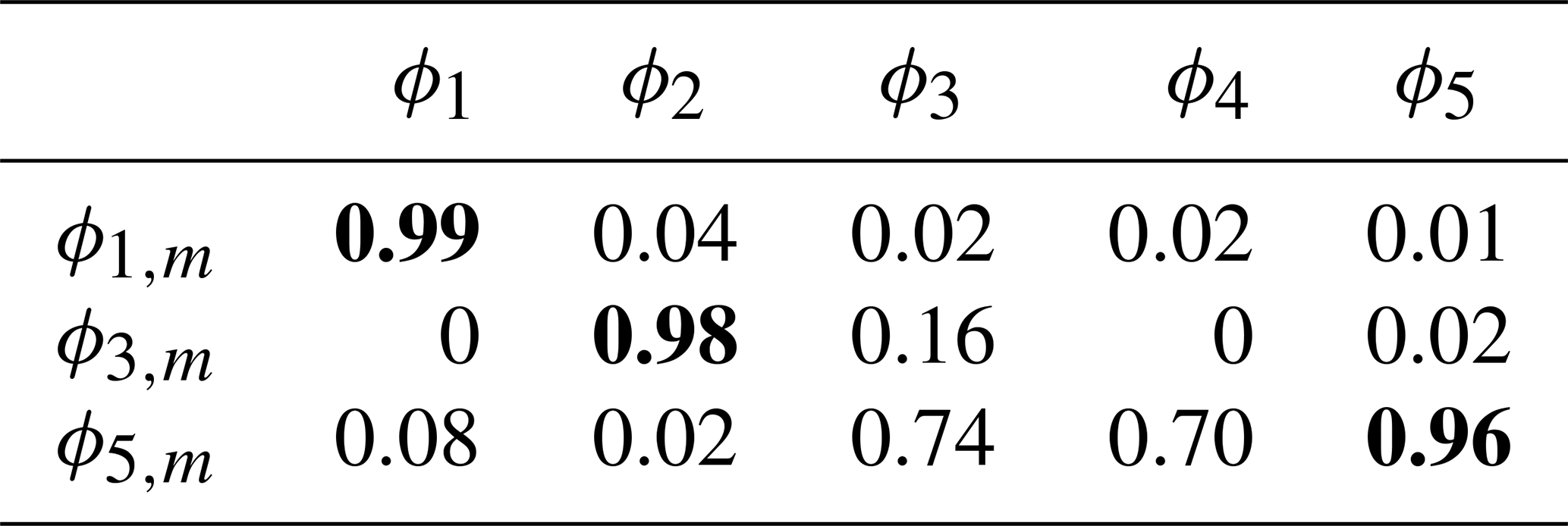
Furthermore, looking at the mode shape ϕ3 and ϕ4 (see Fig. 13c and d), it is observed that the cantilever beam remains approximately straight between 200 and 800 mm. This can be attributed to the additional stiffness which the airfoil adds to the structure. Since the airfoil is only represented as a lumped mass in the FE model, this model cannot accurately capture this effect. The mode shapes ϕ1, ϕ2, and ϕ5 inferred via OMA (see Fig. 13a, b, and f) seem to be the mode shapes most similar to the FE-estimated mode shapes ϕ1,m, ϕ3,m, and ϕ5,m (see Fig. 15). To evaluate this, we compute the modal assurance criterion (MAC), introduced by Allemang and Brown (1982), between the model-based and experimental (from experiment 15; see Fig. 13) mode shapes from the undamaged system. For that purpose, we use the data of the five accelerometers and of the FE model at the same locations. The results shown in Table 5 confirm that the mode shapes ϕ1 and ϕ1,m, ϕ2 and ϕ3,m, and ϕ5 and ϕ5,m are the most similar mode shapes, as these exhibit the highest MAC, given the five vertical degrees of freedom considered in the computation. Also, the corresponding eigenfrequencies of f1≈1.95 Hz and f2≈13.88 Hz and of Hz and Hz are close to each other. However, f5≈44.921 Hz and Hz differ more. Nevertheless, due to the good match for the first two natural frequencies and eigenmodes, we conclude that the simulation model offers a sufficient approximation of the experimental setup and may be used for further analysis.
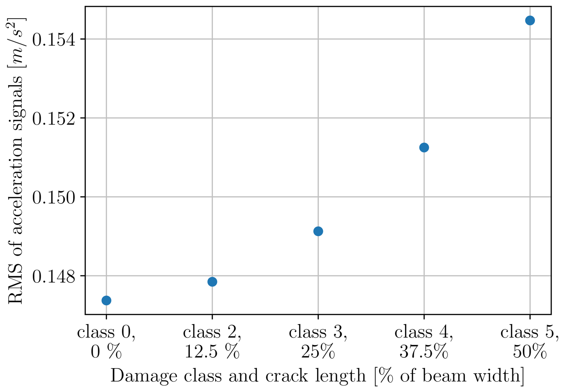
Figure 16RMS of the simulated acceleration response at the location of sensor 5, in the FE model, for all damage classes without an added mass. The system is loaded by a harmonic force with an excitation frequency of fh=1.0 Hz.
Figure 16 reports the evolution of the RMS of the simulated accelerations (in the y direction), recorded at the position of sensor 5 of the FE-based cantilever beam, on the different damage classes without additional mass. The system is loaded by a harmonic excitation with a frequency of 1.0 Hz. In this model, we do not account for the added mass; thus, damage class 1 is missing. In the simulated case, the RMS of the acceleration signal appears to be monotonically increasing with growing crack length. Furthermore, the PSDs of the acceleration signals of sensor 5 of the FE model for all damage classes without added mass are shown in Fig. 17a. The simulated acceleration signals have a sampling frequency of 1000 Hz, and the PSD is computed with Welch's method (Welch, 1967) and the Python implementation in SciPy (Virtanen et al., 2020). Panels (b), (c), and (d) of Fig. 17 show in detail the peaks in the PSDs corresponding to the eigenfrequencies f1,m, f2,m, and f5,m of the model. When examining the first two modes, panels (b) and (c) reveal that, for increasing damage, the peaks in the PSDs shift toward lower frequencies with increasing crack length, meaning that the eigenfrequencies f1,m and f2,m decrease. Moreover, the magnitude (energy) of these peaks seems to uniformly increase, which implies that the vibration amplitudes of these eigenmodes are also increased. For the third vertically oscillating eigenmode in panel (d), the eigenfrequency also appears to decrease with increasing damage, but, unlike the behavior for the first two modes, the magnitude of the peaks does not increase. This last observation implies that the RMS is likely not a concise damage proxy. The model does hint that a (monotonic) decrease in eigenfrequencies is expected for this type of crack, and, indeed, such a decrease is roughly observed in the experimental data. In the experimental forced tests, which aimed to mimic response under wind inflow conditions (Fig. 11), we observe more pronounced variability in the response amplitude and in the variation in the observed frequencies. This can be due to variations in the loading conditions, small variations in the support conditions throughout the experiment, noise (disturbances) due to vibrating sensor cables along the beam, and the measurement noise present in the experimental setup. We particularly expect variations in the excitation frequency to contribute to this variability, since, firstly, we could set these only approximately in the experimental setup (see Sect. 3.3) and, secondly, the second excitation frequency fh=1.9 Hz is quite close to the first natural frequency of the setup and causes resonance effects in the vibrations. The discrepancies exhibited during the experiment are also expected to appear on site under operational conditions. As the resulting damage detection and rating problem is non-trivial, we refrain from using standard unsupervised vibration-based methods as the reference in this case. To tackle the added complexity of utilizing indirect pressure measurements, rather than vibrational (structural) responses, we employ the proposed supervised learning approach. This approach relies on a learning algorithm designed to account for the latent information embedded in the signals during these experiments.
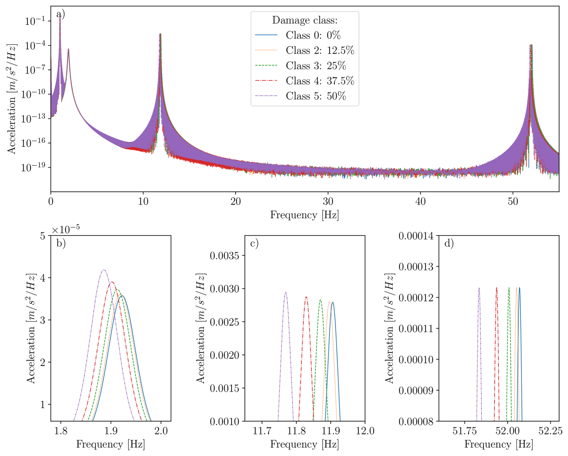
Figure 17Panel (a) displays the PSDs of the acceleration signals extracted at the position of sensor 5 from the simulated structural response of the FE model of all damage states without an additional mass. The simulated signals of sensor 5 are sampled with 1000 Hz. The PSD is calculated with Welch's method (Welch, 1967) and its Python implementation in SciPy (Virtanen et al., 2020). Panel (b) shows the evolution of the peak of f1,m in detail on a linear scale, and panels (c) and (d) show the evolution of the peaks of f2,m and f5,m, respectively. The legend shown in panel (a) is valid for panels (b), (c), and (d) as well.
In this work, we show for the first time that it is possible to detect and rank the severity of structural damage on an elastic, aerodynamically loaded, beam-like structure based solely on measurements of the sectional aerodynamic pressure distribution over a 2D airfoil. To demonstrate this, we conduct a wind tunnel study where an NACA 633418 airfoil is mounted on a heaving cantilever beam. We record the sectional aerodynamic pressure distribution over the airfoil under various boundary conditions, comprising different angles of attack, wind velocities, heaving frequencies, and damage states, using the Aerosense system, a cost-effective and non-intrusive MEMS-based sensing system. We then design a supervised learning algorithm, based on a CNN architecture, for damage detection and severity ranking that uses the measured time series of the sectional aerodynamic pressure distribution as input. The proposed multivariate algorithm achieves a mean classification accuracy of 91.6 % for the 0° AoA dataset and of 89.2 % for the 8° AoA dataset, when averaged over the three considered splits of the respective datasets. Furthermore, we determine with reference acceleration measurements and an FE model of the cantilever beam that the cantilever beam exhibits complex dynamics, with the resulting measured response not revealing purely monotonic trends (e.g., in terms of amplitude increase or frequency shifts), which renders the damage identification problem non-trivial.
Although the two datasets of aerodynamic pressure measurements consequently comprise different wind velocities V, heaving frequencies fh, and complex dynamic behavior of the structure, our proposed deep-learning-based method with only slightly optimized hyperparameters yields good results, with high classification accuracy and narrow-banded confusion matrices for both datasets and all regarded splits. Thus, we conclude that our initial hypothesis that structural damage can be detected and rated based on sectional aerodynamic pressure measurements within a mildly turbulent environment and a fixed-wing setup is indeed valid and that damage detection using aerodynamic pressure measurements from MEMS-based sensing is a path that warrants further investigation for real-world SHM.
For future research on the use of aerodynamic pressure measurements for damage detection, we consider it essential to better understand the transient aerodynamic phenomena caused by increased heaving or pitching amplitudes. A deeper understanding of these phenomena appears to be crucial for detecting damage to WTBs in real-world environmental and operational settings. In addition, we recommend performing similar experiments with a crack orientation that corresponds to a bending damage and under more realistic operational and environmental conditions. Further future work should also focus on applying interpretable machine learning techniques – such as saliency maps, feature attribution methods, or layer-wise relevance propagation – to better understand the features learned by the model. Enhancing interpretability is essential for building trust in data-driven damage indicators and supporting informed decision-making in structural health monitoring, especially if these are based on such indirect proxies for structural damage as aerodynamic pressure measurements.
Besides these immediate next steps, scaling the damage detection approach proposed in this study to full-scale wind turbines and real-world EOCs requires substantial further research and development. We propose the following multi-stage strategy to facilitate this scaling process:
-
Simulation and experimental validation. Further numerical simulations and experimental validation – such as wind tunnel testing using a miniature wind turbine under varying wind speed conditions and turbulence intensities – are essential. These efforts aim to deepen our understanding of how realistic inflow conditions, rotational aerodynamic effects, and real-world damage scenarios influence the pressure distribution along turbine blades. Additionally, more advanced material models and realistic damage representations will be necessary to accurately account for variations in material properties and structural integrity. Future research efforts will aim to translate the proposed methodology to composite specimens to more closely align with practical applications in WTB monitoring.
-
Spatial distribution of pressure sensors. Scaling damage detection to cover the full blade span can be realized by deploying multiple Aerosense sensor nodes along each blade, as illustrated in Fig. 1a of the article. This setup enables the simultaneous acquisition and processing of aerodynamic pressure data at several chord- and span-wise locations, thereby enhancing spatial resolution and detection capability.
-
Unsupervised or self-supervised damage detection. In real-world applications, labeled data are typically unavailable. Therefore, an unsupervised or self-supervised approach to anomaly or damage detection is required. In ongoing work, we are developing such a method tailored to the dataset presented in this study, to be reported in a forthcoming publication. To adapt this to operational and environmental variability, we propose leveraging local inflow information estimated via other Aerosense methods (see Barber et al., 2022; Deparday et al., 2025). Moreover, fusing aerodynamic pressure data with measurements from the 6-DOF inertial measurement unit embedded in each Aerosense node may further enhance robustness and sensitivity.
-
Field deployment and scaling. The final step involves implementing the proposed sensor layout and detection methods on a small-scale operational wind turbine. Field testing will serve to validate the performance of the unsupervised detection framework. The knowledge and insights gained through this process will inform the subsequent upscaling to full-scale wind turbines, enabling robust aerodynamic-pressure-based damage detection under realistic conditions.
Moreover, another future research direction consists of quantitative comparison between pressure-based and conventional vibration-based damage indicators. Although, from a purely diagnostic standpoint, vibration-based features may offer superior performance in many scenarios, aerodynamic-pressure-based indicators might offer a pragmatic and scalable option for structural health monitoring in environments where access to direct structural measurements is limited. Hence, a quantitative comparison to assess the trade-offs between these sensing approaches would offer valuable insights.
Finally, another interesting application scenario, beyond wind turbines, for the Aerosense measurement system and for aerodynamic-pressure-based damage detection, consists of slender, long-span suspension bridges. For such bridges, excitation by wind loading and thus aerodynamic pressure plays an essential role (Fenerci and Øiseth, 2017; Civera et al., 2024; Kvåle et al., 2023). Here, the Aerosense system could contribute not only by monitoring the wind loading at selected points, but also by enhancing existing acceleration-based damage detection methods by information derived from aerodynamic pressure data.
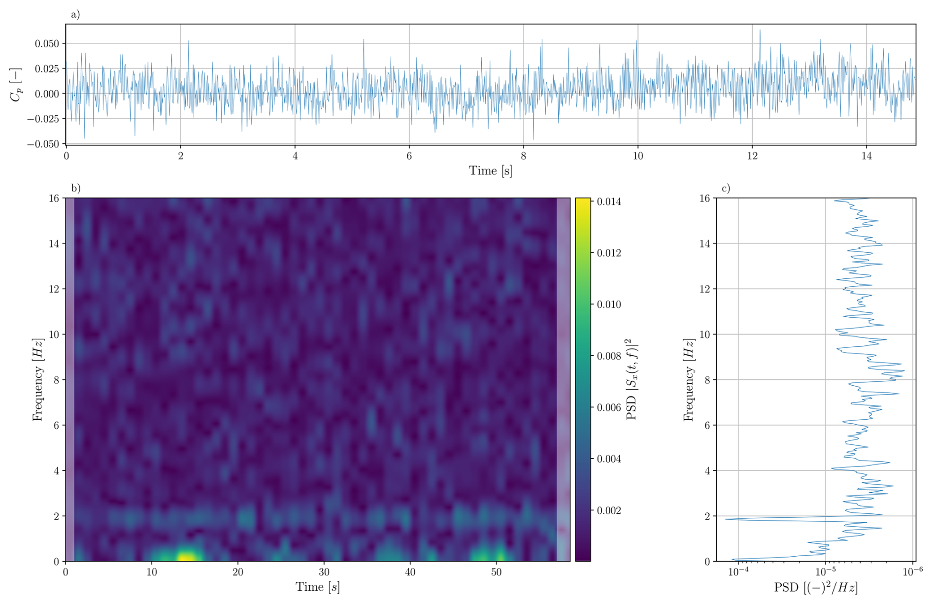
Figure A1(a) Extract of the pressure time history recorded by sensor 14, located at on the suction side of the airfoil, with 8° AoA under V=24 m s−1 and fh=1.9 Hz in experiment 16. Panel (b) shows how the spectrum of the pressure time history of sensor 14 of experiment 16 with 8° AoA varies over the whole duration of the experiment via a spectrogram. The spectrogram is computed using the discrete short-term Fourier transformation of SciPy (Virtanen et al., 2020). The shaded areas at the left and right ends of the spectrum indicate areas affected by sliding windows that are partially outside of the analyzed signal Panel (c) depicts the PSD of the same signal computed over the whole duration of experiment 16 and is calculated with Welch's method and its implementation in SciPy (Virtanen et al., 2020).
Table A1Overview of experiments and their boundary conditions. The entries in columns 1, 2, and 3 are the identifiers of the measurements conducted under the boundary conditions of the same row. This numbering is applied for both the 0 and 8° AoA datasets.
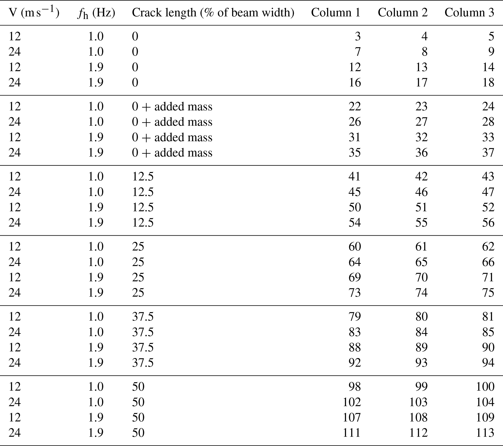
Table A2Overview of experiments where only harmonic forces are acting on the cantilever beam. This numbering is applied for both the 0 and 8° AoA datasets.
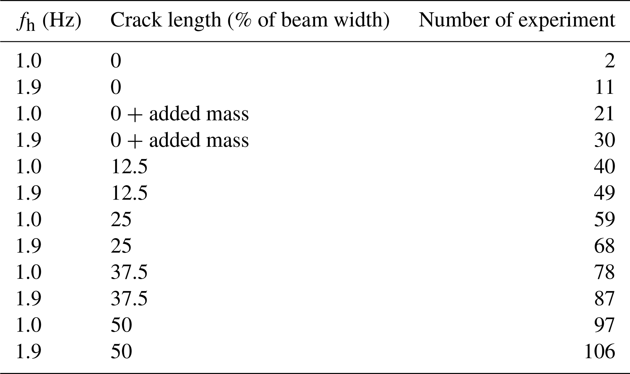
Table A3Eigenfrequencies fi,m (in Hz) of the first five eigenmodes ϕi,m of the FE model, determined via eigenvalue analysis.
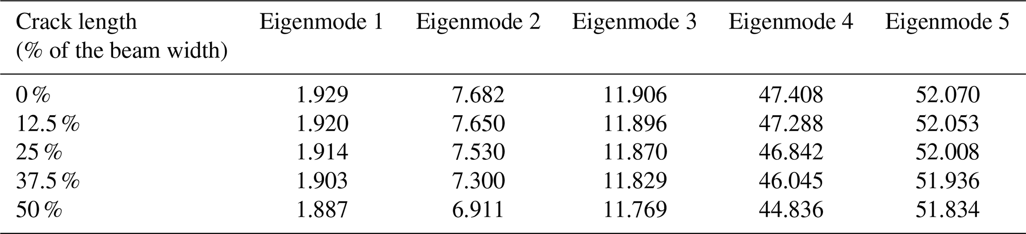
Table A4Natural frequencies fi of the modes found with AFDD and clustering below 60 Hz, described by their mean μf,i and standard deviation σf,i, for all structural states and rounded to three decimal digits. The eigenfrequencies fi are associated only with the vertically oscillating eigenmodes of the cantilever beam.
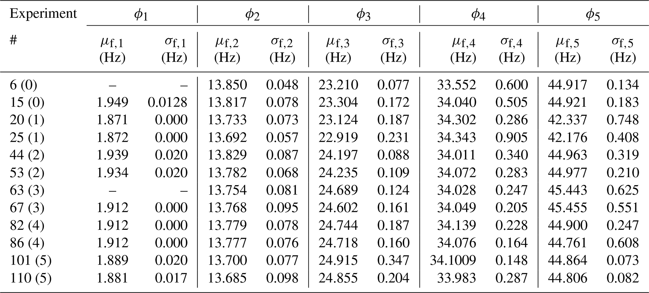
The data of our experiments are available in the following repository: https://doi.org/10.34808/gq12-wx33 (Abdallah et al., 2023).
The code being developed within this publication is available on Zenodo: https://doi.org/10.5281/zenodo.17911886 (Franz et al., 2025).
PF: methodology, investigation, data analysis, software, visualization, writing (original draft and review and editing). IA: conceptualization, design of experiments and wind tunnel setup, conduction of experiments, methodology, supervision, writing (theory supporting hypothesis in Sect. 2.1 and review and editing). GD: conceptualization, design of experiments and wind tunnel setup, conduction of experiments, methodology, data analysis, software, supervision, writing (review and editing). JD: conceptualization, wind tunnel setup and experiments, methodology, software, supervision, writing (review and editing). AJ: finite element modeling, writing (description of finite element model). XJ: data analysis, software, writing (review and editing). MD: methodology, supervision, writing (review and editing). AP: methodology, supervision, resources, writing (review and editing). SB: Aerosense project lead, conceptualization, resources, writing (review and editing). EC: conceptualization, methodology, software, resources, supervision, writing (review and editing).
The contact author has declared that none of the authors has any competing interests.
Publisher's note: Copernicus Publications remains neutral with regard to jurisdictional claims made in the text, published maps, institutional affiliations, or any other geographical representation in this paper. While Copernicus Publications makes every effort to include appropriate place names, the final responsibility lies with the authors. Views expressed in the text are those of the authors and do not necessarily reflect the views of the publisher.
The authors gratefully acknowledge and thank Karen Mulleners, head of the Unsteady Flow Diagnostics Laboratory (UNFoLD), from EPFL for providing the wind tunnel and supporting our experiments. Alexander Popp acknowledges support by dtec.bw – Digitalization and Technology Research Center of the Bundeswehr (project RISK.twin). dtec.bw is funded by the European Union – Next GenerationEU. Moreover, the authors gratefully acknowledge the computational resources provided through the joint high-performance data analytics (HPDA) project “terrabyte” of the German Aerospace Center (DLR) and the Leibniz Supercomputing Center (LRZ).
This research has been supported by the Schweizerischer Nationalfonds zur Förderung der Wissenschaftlichen Forschung (grant no. 200021L_212718, project MISTERY – Modelling and estimation of unsteady aerodynamic flow at high Reynolds number) and by the BRIDGE Discovery program of the Swiss National Science Foundation and Innosuisse (grant no. 40B2−0_187087, project AEROSENSE).
This paper was edited by Michael Muskulus and reviewed by two anonymous referees.
Abdallah, I., Deparday, J., Marykovskiy, Y., and Barber, S.: AeroSense Measurements: Wind Tunnel EPFL (1–), Gdańsk University of Technology [data set], https://doi.org/10.34808/gq12-wx33, 2023. a
Abadi, M., Agarwal, A., Barham, P., Brevdo, E., Chen, Z., Citro, C., Corrado, G. S., Davis, A., Dean, J., Devin, M., Ghemawat, S., Goodfellow, I., Harp, A., Irving, G., Isard, M., Jia, Y., Jozefowicz, R., Kaiser, L., Kudlur, M., Levenberg, J., Mané, D., Monga, R., Moore, S., Murray, D., Olah, C., Schuster, M., Shlens, J., Steiner, B., Sutskever, I., Talwar, K., Tucker, P., Vanhoucke, V., Vasudevan, V., Viégas, F., Vinyals, O., Warden, P., Wattenberg, M., Wicke, M., Yu, Y., and Zheng, X.: TensorFlow: Large-Scale Machine Learning on Heterogeneous Systems, https://www.tensorflow.org/ (last access: 12 December 2025), 2015. a
Abdi, S., Mani, M., Ajalli, F., and Soltani, M. R.: Unsteady surface pressure measurement on a pitching air foil, 6th International Conference on Heat Transfer, Fluid Mechanics and Thermodynamics, Pretoria, South Africa, 30 June–2 July 2008, http://hdl.handle.net/2263/40005 (last access: 31 October 2024), 2008. a, b
Ajalli, F., Mani, M., and Soltani, M. R.: An experimental investigation of pressure distribution around a heaving airfoil [conference paper], 5th International Conference on Heat Transfer, Fluid Mechanics and Thermodynamics, Sun City, South Africa, 1–4 July 2007, http://hdl.handle.net/2263/40993 (last access: 31 October 2024), 2007. a, b
Allemang, R. J. and Brown, D. L.: A correlation coefficient for modal vector analysis, in: 1st International Modal Analysis Conference, Society for Experimental Mechanics, Orlando, FLorida, USA, 110–116, 1982. a
Anderson, J. D.: Fundamentals of aerodynamics, McGraw-Hill series in aeronautical and aerospace engineering, McGraw-Hill Education, New York, NY, 6yh edn., ISBN 1259129918, 2017. a
Avendaño-Valencia, L. D., Chatzi, E. N., and Tcherniak, D.: Gaussian process models for mitigation of operational variability in the structural health monitoring of wind turbines, Mechanical Systems and Signal Processing, 142, 106686, https://doi.org/10.1016/j.ymssp.2020.106686, 2020. a
Barber, S., Deparday, J., Marykovskiy, Y., Chatzi, E., Abdallah, I., Duthé, G., Magno, M., Polonelli, T., Fischer, R., and Müller, H.: Development of a wireless, non-intrusive, MEMS-based pressure and acoustic measurement system for large-scale operating wind turbine blades, Wind Energ. Sci., 7, 1383–1398, https://doi.org/10.5194/wes-7-1383-2022, 2022. a, b, c, d, e
Blevins, R. D.: Flow-induced Vibration, Van Nostrand Reinhold, New York, NY, 2nd edn., ISBN 0442206518, 1990. a, b
Brincker, R. and Ventura, C. E. H.: Introduction to operational modal analysis, John Wiley and Sons Inc, Chichester, West Sussex, ISBN 978-1-119-96315-8, https://doi.org/10.1002/9781118535141, 2015. a
Brincker, R., Zhang, L., and Andersen, P.: Modal Identification from Ambient Responses using Frequency Domain Decomposition, in: IMAC 18 : Proceedings of the International Modal Analysis Conference (IMAC), San Antonio, Texas, USA, 7–10 February 2000, 625–630, the International Modal Analysis Conference, 2000. a
Brincker, R., Ventura, C., and Andersen, P.: Damping Estimation by Frequency Domain Decomposition, in: Proceedings of IMAC 19, 698–703, Society for Experimental Mechanics, United States, the International Modal Analysis Conference, 5–8 February 2001, 2001a. a
Brincker, R., Zhang, L., and Andersen, P.: Modal identification of output-only systems using frequency domain decomposition, Smart Materials and Structures, 10, 441, https://doi.org/10.1088/0964-1726/10/3/303, 2001b. a
Brondsted, P., Nijssen, Rogier P. L., and Goutianos, S. (Eds.): Advances in Wind Turbine Blade Design and Materials, Elsevier Science & Technology, San Diego, ISBN 9780081030080, 2023. a
Chandrasekhar, K., Stevanovic, N., Cross, E. J., Dervilis, N., and Worden, K.: Damage detection in operational wind turbine blades using a new approach based on machine learning, Renewable Energy, 168, 1249–1264, https://doi.org/10.1016/j.renene.2020.12.119, 2021. a
Cheynet, E., Jakobsen, J. B., and Snæbjörnsson, J.: Damping estimation of large wind-sensitive structures, Procedia Engineering, 199, 2047–2053, https://doi.org/10.1016/j.proeng.2017.09.471, 2017. a
Chollet, F. and others: Keras, https://keras.io (last access: 12 December 2025), 2015. a
Ciang, C. C., Lee, J.-R., and Bang, H.-J.: Structural health monitoring for a wind turbine system: a review of damage detection methods, Measurement Science and Technology, 19, 122001, https://doi.org/10.1088/0957-0233/19/12/122001, 2008. a
Civera, M., Rosso, M. M., Marano, G. C., and Chiaia, E.: Validation and Comparison of Two AOMA Approaches for the Ambient Vibration Testing of Long Suspension Bridges Under Strong Wind Loads, in: Proceedings of the 10th International Operational Modal Analysis Conference (IOMAC 2024), edited by: Rainieri, C., Gentile, C., and Aenlle López, M., 475–484, Springer Nature Switzerland, Cham, ISBN 978-3-031-61425-5, 2024. a
Deparday, J., Müller, H., Polonelli, T., and Barber, S.: An experimental system to acquire aeroacoustic properties on wind turbine blades, Journal of Physics: Conference Series, 2265, 022089, https://doi.org/10.1088/1742-6596/2265/2/022089, 2022. a
Deparday, J., Marikovskiy, Y., Abdallah, I., and Barber, S.: An aerodynamic measurement system to improve the efficiency of wind turbine rotor blades, arxiv [preprint], https://arxiv.org/abs/2503.08860 (last access: 12 December 2025), 2025. a
Diken, H. and Asiri, S.: Parametric study of flapwise and edgewise vibration of horizontal axis wind turbine blades, Advances in Mechanical Engineering, 13, 168781402110508, https://doi.org/10.1177/16878140211050801, 2021. a
Di Lorenzo, E., Petrone, G., Manzato, S., Peeters, B., Desmet, W., and Marulo, F.: Damage detection in wind turbine blades by using operational modal analysis, Structural Health Monitoring, 15, 289–301, https://doi.org/10.1177/1475921716642748, 2016. a
Duthé, G., Abdallah, I., Barber, S., and Chatzi, E.: Modeling and monitoring erosion of the leading edge of wind turbine blades, Energies, 14, 7262, https://doi.org/10.1088/1742-6596/2265/2/022074, 2021. a
Fenerci, A. and Øiseth, O.: The Hardanger Bridge monitoring project: Long-term monitoring results and implications on bridge design, Procedia Engineering, 199, 3115–3120, https://doi.org/10.1016/j.proeng.2017.09.576, 2017. a
Franz, P., Abdallah, I., Duthé, G., Deparday, J., Jafarabadi, A., Jian, X., von Danwitz, M., Popp, A., Barber, S., and Chatzi, E.: Code for `On the Potential of Aerodynamic Pressure Measurements for Structural Damage Detection' (v1.0.0), Zenodo [code], https://doi.org/10.5281/zenodo.17911886, 2025. a
García, D. and Tcherniak, D.: An experimental study on the data-driven structural health monitoring of large wind turbine blades using a single accelerometer and actuator, Mechanical Systems and Signal Processing, 127, 102–119, https://doi.org/10.1016/j.ymssp.2019.02.062, 2019. a
Global Wind Energy Council: Global Wind Report 2023, Tech. rep., https://gwec.net/globalwindreport2023/, last access: 17 January 2024, 2023. a
Glorot, X. and Bengio, Y.: Understanding the difficulty of training deep feedforward neural networks, in: Proceedings of the Thirteenth International Conference on Artificial Intelligence and Statistics, vol. 9, 249–256, PMLR, Chia Laguna Resort, Sardinia, Italy, 2010. a
Hodges, D. H. and Pierce, G. A.: Introduction to structural dynamics and aeroelasticity, vol. 15, Cambridge University Press, Cambridge, 2nd edn., 2011. a
Hu, H. and Yang, Z.: An Experimental Study of the Laminar Flow Separation on a Low-Reynolds-Number Airfoil, Journal of Fluids Engineering, 130, https://doi.org/10.1115/1.2907416, 2008. a
Ismail Fawaz, H., Forestier, G., Weber, J., Idoumghar, L., and Muller, P.-A.: Deep learning for time series classification: a review, Data Mining and Knowledge Discovery, 33, 917–963, https://doi.org/10.1007/s10618-019-00619-1, 2019. a, b, c, d, e, f, g
Kaewniam, P., Cao, M., Alkayem, N. F., Li, D., and Manoach, E.: Recent advances in damage detection of wind turbine blades: A state-of-the-art review, Renewable and Sustainable Energy Reviews, 167, 112723, https://doi.org/10.1016/j.rser.2022.112723, 2022. a
Kingma, D. P. and Ba, J.: Adam: A Method for Stochastic Optimization, in: Proceedings of the 3rd International Conference on Learning Representations, ICLR, San Diego, USA, 7–9 May 2015, https://doi.org/10.48550/arXiv.1412.6980, 2015. a
Kong, K., Dyer, K., Payne, C., Hamerton, I., and Weaver, P. M.: Progress and Trends in Damage Detection Methods, Maintenance, and Data-driven Monitoring of Wind Turbine Blades – A Review, Renewable Energy Focus, 44, 390–412, https://doi.org/10.1016/j.ref.2022.08.005, 2023. a
Kvåle, K. A., Fenerci, A., Øyvind Wiig Petersen, Rønnquist, A., and Øiseth, O.: Data Set from Long-Term Wave, Wind, and Response Monitoring of the Bergsøysund Bridge, Journal of Structural Engineering, 149, 04723002, https://doi.org/10.1061/JSENDH.STENG-12095, 2023. a
Laflamme, S., Cao, L., Chatzi, E., and Ubertini, F.: Damage Detection and Localization from Dense Network of Strain Sensors, Shock and Vibration, 2016, 1–13, https://doi.org/10.1155/2016/2562949, 2016. a, b
LeCun, Y., Bengio, Y., and Hinton, G.: Deep learning, Nature, 521, 436–444, https://doi.org/10.1038/nature14539, 2015. a, b, c
Lloyd, S.: Least squares quantization in PCM, IEEE Transactions on Information Theory, 28, 129–137, https://doi.org/10.1109/TIT.1982.1056489, 1982. a
Madsen, H. A., Barlas, T., Fischer, A., Olsen, A. S., and Gomez Gonzalez, A.: Inflow and pressure measurements on a full scale turbine with a pressure belt and a five hole pitot tube, Journal of Physics: Conference Series, 2265, 022096, https://doi.org/10.1088/1742-6596/2265/2/022096, 2022. a
Marykovskiy, Y., Deparday, J., Abdallah, I., Duthé, G., Barber, S., and Chatzi, E.: Hybrid Model for Inflow Conditions Inference on Airfoils Under Uncertainty, AIAA Journal, 61, 4913–4925, https://doi.org/10.2514/1.J063108, 2023. a
MATLAB: version '9.11.0.2358333 (R2021b) Update 7', The MathWorks Inc., Natick, Massachusetts, 2021. a
Mishnaevsky, L.: Root Causes and Mechanisms of Failure of Wind Turbine Blades: Overview, Materials, 15, https://doi.org/10.3390/ma15092959, 2022. a
Modarres-Sadeghi, Y., ed.: Introduction to Fluid-Structure Interactions, Springer International Publishing and Imprint Springer, Cham, 1st edn. 2021, ISBN 978-3-030-85882-7, https://doi.org/10.1007/978-3-030-85884-1, 2021. a, b
Mohammadi Foumani, N., Miller, L., Tan, C. W., Webb, G. I., Forestier, G., and Salehi, M.: Deep Learning for Time Series Classification and Extrinsic Regression: A Current Survey, ACM Computing Surveys, 56, 1–45, https://doi.org/10.1145/3649448, 2024. a
Musial, W., Spitsen, P., Beiter, P., Duffy, P., Mulas Hernando, D., Hammond, R., Shields, M., and Marquis, M.: Offshore Wind Market Report: 2023 Edition [Slides], United States, 2023, https://doi.org/10.2172/1997466, 2023. a
Ou, Y., Tatsis, K. E., Dertimanis, V. K., Spiridonakos, M. D., and Chatzi, E. N.: Vibration-based monitoring of a small-scale wind turbine blade under varying climate conditions. Part I: An experimental benchmark, Structural control & health monitoring, 28, e2660, https://doi.org/10.1002/stc.2660, 2021. a
Pacheco-Chérrez, J. and Probst, O.: Vibration-based damage detection in a wind turbine blade through operational modal analysis under wind excitation, Materials Today: Proceedings, 56, 291–297, https://doi.org/10.1016/j.matpr.2022.01.159, 2022. a
Pacheco-Chérrez, J., Cárdenas, D., Delgado-Gutiérrez, A., and Probst, O.: Operational modal analysis for damage detection in a rotating wind turbine blade in the presence of measurement noise, Composite Structures, 321, 117298, https://doi.org/10.1016/j.compstruct.2023.117298, 2023. a
Polonelli, T., Deparday, J., Müller, H., Fischer, R., Benini, L., Barber, S., and Magno, M.: Aerosense: Long-Range Bluetooth Wireless Sensor Node for Aerodynamic Monitoring on Wind Turbine Blades, Journal of Physics: Conference Series, 2265, 022074, https://doi.org/10.1088/1742-6596/2265/2/022074, 2022. a, b
Polonelli, T., Müller, H., Kong, W., Fischer, R., Benini, L., and Magno, M.: Aerosense: A Self-Sustainable and Long-Range Bluetooth Wireless Sensor Node for Aerodynamic and Aeroacoustic Monitoring on Wind Turbines, IEEE Sensors Journal, 23, 715–723, https://doi.org/10.1109/JSEN.2022.3224307, 2023. a
Ruangwiset, A. and Suwantragul, B.: Wind tunnel test of UAV fault detection using principal component based aerodynamic model, in: 2008 International Conference on Mechatronics and Automation, 150–154, IEEE, Piscataway, NJ, ISBN 978-1-4244-2631-7, https://doi.org/10.1109/ICMA.2008.4798742, 2008. a
Stehly, T., Beiter, P., and Duffy, P.: 2019 Cost of Wind Energy Review, https://doi.org/10.2172/1756710 (last access: 19 January 2024), 2020. a
Traub, L. W. and Cooper, E.: Experimental Investigation of Pressure Measurement and Airfoil Characteristics at Low Reynolds Numbers, Journal of Aircraft, 45, 1322–1333, https://doi.org/10.2514/1.34769, 2008. a
Veers, P., Bottasso, C. L., Manuel, L., Naughton, J., Pao, L., Paquette, J., Robertson, A., Robinson, M., Ananthan, S., Barlas, T., Bianchini, A., Bredmose, H., Horcas, S. G., Keller, J., Madsen, H. A., Manwell, J., Moriarty, P., Nolet, S., and Rinker, J.: Grand challenges in the design, manufacture, and operation of future wind turbine systems, Wind Energ. Sci., 8, 1071–1131, https://doi.org/10.5194/wes-8-1071-2023, 2023. a, b
Veilleux, J.-C.: Optimization of a Fully-Passive Flapping-Airfoil Turbine, [master thesis], Université Lavale, https://doi.org/10.13140/RG.2.2.36533.58085, 2014. a
Virtanen, P., Gommers, R., Oliphant, T. E., Haberland, M., Reddy, T., Cournapeau, D., Burovski, E., Peterson, P., Weckesser, W., Bright, J., van der Walt, S. J., Brett, M., Wilson, J., Millman, K. J., Mayorov, N., Nelson, A. R. J., Jones, E., Kern, R., Larson, E., Carey, C. J., Polat, İ., Feng, Y., Moore, E. W., VanderPlas, J., Laxalde, D., Perktold, J., Cimrman, R., Henriksen, I., Quintero, E. A., Harris, C. R., Archibald, A. M., Ribeiro, A. H., Pedregosa, F., van Mulbregt, P., and SciPy 1.0 Contributors: SciPy 1.0: Fundamental Algorithms for Scientific Computing in Python, Nature Methods, 17, 261–272, https://doi.org/10.1038/s41592-019-0686-2, 2020. a, b, c, d, e, f, g, h
Wang, Z., Yan, W., and Oates, T.: Time series classification from scratch with deep neural networks: A strong baseline, in: 2017 International Joint Conference on Neural Networks (IJCNN), 1578–1585, IEEE, ISBN 978-1-5090-6182-2, https://doi.org/10.1109/IJCNN.2017.7966039, 2017. a, b, c, d, e
Weijtjens, W., Verbelen, T., Capello, E., and Devriendt, C.: Vibration based structural health monitoring of the substructures of five offshore wind turbines, Procedia Engineering, 199, 2294–2299, https://doi.org/10.1016/j.proeng.2017.09.187, 2017. a
Welch, P.: The use of fast Fourier transform for the estimation of power spectra: A method based on time averaging over short, modified periodograms, IEEE Transactions on Audio and Electroacoustics, 15, 70–73, 1967. a, b
Wiser, R., Bolinger, M., Hoen, B., Millstein, D., Rand, J., Barbose, G., Darghouth, N., Gorman, W., Jeong, S., O'Shaughnessy, E., and Paulos, B.: Land-Based Wind Market Report: 2023 Edition, United States, 2023, https://doi.org/10.2172/1996790, 2023. a
Zhang, Y., de Visser, C. C., Chu, Q. P., and van Kampen, E. J.: Aircraft Damage Pattern Recognition Using Aerodynamic Coefficients and Fuzzy Logic, in: Advances in aerospace guidance, navigation and control, edited by: Dołęga, B., Głębocki, R., Kordos, D., and Żugaj, M., 335–348, Springer, Cham, ISBN 978-3-319-65282-5, https://doi.org/10.1007/978-3-319-65283-2_18, 2018. a
With “heaving airfoil”, we refer to a vertically oscillating airfoil.
- Abstract
- Introduction
- Method and limitations
- Wind tunnel experiments
- Data analysis
- Results
- Discussion: analysis of system dynamics based on acceleration measurements
- Conclusions
- Appendix A
- Data availability
- Code availability
- Author contributions
- Competing interests
- Disclaimer
- Acknowledgements
- Financial support
- Review statement
- References