Spatial development of planar and axisymmetric wakes of porous objects under a pressure gradient: a wind tunnel study

We report an experimental study on the effect of a constant adverse pressure gradient on the spatial evolution of turbulent wakes generated by different objects. A porous disc, designed to mimic the wake of a horizontal-axis wind turbine, and a porous cylinder, whose wake matches that of a vertical-axis wind turbine, were tested in a wind tunnel for Reynolds numbers (based on the generator diameter) in the range of 2.6×10⁵ to 3.9×10⁵. Experiments were conducted between 1 and 7 diameters downstream of the disc and from 2 to 12 diameters downstream of the cylinder.

We find that the effect of the adverse pressure gradient is significant in all cases, resulting in larger velocity deficits and wider wakes. Moreover, these variations are stronger for the cylinder-generated wake. We also find that current analytical models for wakes evolving in pressure gradients, developed from momentum conservation, satisfactorily fit our data. Our results provide a benchmark case that will contribute to improving energy harvesting in cases where pressure gradients are relevant, such as in wind plants installed over complex topographies and tidal stream generators.

1 Introduction

Turbulent flows play a relevant role in several environmental and industrial situations. For instance, within wind farms, the energy loss in the wake of a wind turbine reduces the available power for downstream turbines. Therefore, in order to minimize these losses and design an optimal wind farm layout, it is essential to accurately model the turbulent wakes of wind turbines (Neunaber et al., 2022b; Kadum et al., 2020). Furthermore, in order to predict the power production of wind farms, understanding and modelling their interaction with the atmospheric boundary layer are needed. This interaction defines the entrainment of energy into the wakes of the wind turbines (Stevens and Meneveau, 2017).

Despite decades of intensive studies, even the modelling of averaged statistics of velocity and other quantities (such as Reynolds stresses and dissipation) remains an open question (Johansson et al., 2003; Nedic et al., 2013). For instance, the existence of turbulent wakes with non-canonical energy cascades that result in modifications to the streamwise scaling of the averaged velocity deficit and the wake width has recently been reported (Neunaber et al., 2022b; Ortiz-Tarin et al., 2021). Moreover, several aspects of this flow, particularly relevant for wind energy applications, are still under debate, such as the influence of the background flow and the characteristics of the testing facility (Aubrun et al., 2019; Biswas and Buxton, 2024; Hearst et al., 2016), the spatial extent of the turbulence production region and the near wake (Neunaber et al., 2024; Vahidi and Porté-Agel, 2022; Gambuzza and Ganapathisubramani, 2023), and how the latter is modified by the operating conditions of the rotor (Bourhis and Buxton, 2024; Neunaber et al., 2022a; Scott et al., 2024).

In this context, in many important situations, turbulent wakes evolve within a pressure gradient (Hill et al., 1963; Liu et al., 2002). For instance, wind plants installed over complex topographies and tidal stream generators are expected to be potentially affected by pressure gradients that modify the structure and persistence of the wakes. Consequently, the problem has received renewed attention in recent years (van der Deijl et al., 2022; Cheng et al., 2024). Predictions for the streamwise evolution of the normalized averaged velocity deficit and the wake width have been proposed for planar (Shamsoddin and Porté-Agel, 2017) and axisymmetric (Shamsoddin and Porté-Agel, 2018) turbulent wakes. Furthermore, these proposed scalings have been verified experimentally and numerically for cylinders, discs, and scaled wind turbines (Dar and Porté-Agel, 2022; Dar et al., 2023; Dar and Porté-Agel, 2024).

In this work, we report a wind tunnel study using porous actuators to further characterize the effect of an adverse pressure gradient (APG) on vertical- and horizontal-axis wind turbine wakes (VAWTs and HAWTs, respectively). Indeed, porous plates have been found to properly match several averaged properties of HAWT wakes (Aubrun et al., 2013, 2019; Camp and Cal, 2016; Vinnes et al., 2022) and even their higher-order statistics (Vinnes et al., 2023; Neunaber et al., 2020). On the other hand, VAWTs have also been modelled as porous cylinders (Steiros et al., 2020; Ning, 2016). We remark, nevertheless, that in the present study the cylinder only emulates a VAWT with a very large aspect ratio since the cylinder spans the full height of the wind tunnel. The aspect ratio of a VAWT is important for the development of the wake (Araya et al., 2017), so this cylinder is not a perfect representation of a VAWT wake.

We present a systematic study in which a porous disc and a porous cylinder are characterized within a streamwise zero-pressure gradient (ZPG) and an APG. Both generators are tested at three different Reynolds numbers (${\mathit{Re}}_D=U_{\mathrm{\infty }}D/\mathit{\nu }$, with U_∞ being the freestream velocity, ν the kinematic viscosity, and D the diameter of the disc or cylinder) in the range $\mathrm{2.6}\times {\mathrm{10}}^{\mathrm{5}}-\mathrm{3.9}\times {\mathrm{10}}^{\mathrm{5}}$. They are also designed to have similar values of thrust coefficients C_T that match realistic rotors.

To this aim, the wake generator can be placed in the normal test section of the wind tunnel (with a negligible pressure gradient) or in the diffuser section, where a constant APG is present in the flow. The wind tunnel has a long diffuser section, allowing for the study of the wake's evolution at least 7 diameters downstream of its generator. It, therefore, covers a range that is pertinent for wind energy applications, particularly concerning turbine layouts within a farm. Furthermore, we consider one case where the generator is placed in the test section, and the wake evolves within it and then continues through the diffuser. Consequently, our work covers both a situation in which a self-similar turbulent wake faces a pressure gradient and a situation in which both the near and the far wakes evolve within the APG.

The relevance of this study lies in the comparison, at relatively large values of Re_D, of the turbulent wakes of porous cylinders and discs. Our results, obtained in the same tunnel, can be used and adapted to the design of HAWTs and VAWTs in the presence of pressure gradients. They also allow us to evaluate how different the effect of an APG is for both types of rotors, as experiments are performed in the same facility and using the same collection techniques. Our experimental results are also compared with available analytical models for turbulent wakes within an APG (discussed in detail in Sect. 2; see also, for instance, Shamsoddin and Porté-Agel, 2018, and Shamsoddin and Porté-Agel, 2017), finding satisfactory agreement between them.

The present paper is organized as follows. Section 2 summarizes the models from the literature that describe the streamwise evolution of turbulent wakes in the presence of a pressure gradient (Shamsoddin and Porté-Agel, 2017, 2018). Section 3 details the experimental setup, including the wind tunnel used for the tests, the tested objects, and how velocity profiles were obtained. Section 4 discusses the effect of the APG depending on the type of generator. In Sect. 5, the influence of the pressure gradient in the turbulent wakes is evaluated following the models from the literature. Finally, Sect. 6 states the conclusions and perspectives raised by this work.

2 Theory: streamwise evolution of turbulent wakes in an adverse pressure gradient

The theory that models the far turbulent wake always requires self-similarity of the averaged streamwise velocity deficit (Bastankhah and Porté-Agel, 2014). Additionally, further terms from the momentum or kinetic energy balances can be modelled if this property is imposed on other quantities (George, 1989; Townsend, 1976). In the following, we briefly detail the models available to describe the evolution of a turbulent wake within a ZPG and in the presence of an APG. We remark that, while in the present work only a constant APG is considered, the models detailed below work for any type of pressure gradient (including adverse or favourable conditions).

2.1 Axisymmetric wake

In the case of a self-similar axisymmetric wake, the mean velocity deficit can be appropriately described by a Gaussian profile (Pope, 2000) such that

$$\begin{array}{}\text{(1)}& {\displaystyle \frac{U_{\mathrm{b}}\left(x\right)-\stackrel{\mathrm{‾}}{u}\left(x,r\right)}{U_{\mathrm{b}}\left(x\right)}}\equiv C\left(x\right){\mathrm{e}}^{-\left(r^{\mathrm{2}}/\mathrm{2}{\mathit{\delta }}^{\mathrm{2}}\right)},\end{array}$$

where U_b is the base flow velocity that can vary in the streamwise direction x as a result of a pressure gradient, and $\stackrel{\mathrm{‾}}{u}$ is the averaged streamwise velocity at the streamwise distance x and a radial distance from the wake centre r. C(x) is therefore the centreline (and maximum) velocity deficit in the wake, and δ(x) is the wake width.

Shamsoddin and Porté-Agel (2018) derived a nonlinear ordinary differential equation (ODE) from the conservation of the averaged momentum equation for an axisymmetric wake, in which the inviscid terms have been neglected, including a pressure gradient in the x direction,

$$\begin{array}{}\text{(2)}& \begin{array}{rl}{\displaystyle \frac{\mathrm{d}C\left(x\right)}{\mathrm{d}x}}& ={\displaystyle \frac{-\mathrm{1}}{\left(\frac{U_{\mathrm{b}}^{\mathrm{4}}\left(x\right)}{{\mathit{\lambda }}_{\mathrm{0}}^{\mathrm{2}}\left(x\right)}\right)\left(\mathrm{3}{C}^{\mathrm{2}}\left(x\right)-\mathrm{2}{C}^{\mathrm{3}}\left(x\right)\right)}}\\ & \left[{\displaystyle \frac{\mathrm{1}}{\mathrm{4}}}{\displaystyle \frac{\mathrm{d}{U}_{\mathrm{b}}^{\mathrm{4}}\left(x\right)}{\mathrm{d}x}}{\displaystyle \frac{C^{\mathrm{3}}\left(x\right)}{{\mathit{\lambda }}_{\mathrm{0}}^{\mathrm{2}}\left(x\right)}}+\left(C^{\mathrm{3}}\left(x\right)-{\displaystyle \frac{C^{\mathrm{4}}\left(x\right)}{\mathrm{2}}}\right){\displaystyle \frac{\mathrm{d}}{\mathrm{d}x}}\left({\displaystyle \frac{U_{\mathrm{b}}^{\mathrm{4}}\left(x\right)}{{\mathit{\lambda }}_{\mathrm{0}}\left(x\right)}}\right)\right],\end{array}\end{array}$$

where λ₀(x) is the ratio between the velocity deficit and wake width. This ratio λ₀(x) is assumed to be independent of the pressure gradient (see Eq. 4). The subscript 0 indicates a quantity in the ZPG. The subscript i refers to the smallest x position within the pressure gradient, and it is where the boundary condition, i.e. the starting point, is applied to the ODE. The boundary condition for this ODE is set to be

$$\begin{array}{}\text{(3)}& C\left(x_i\right)=C_{\mathrm{0}}\left(x_i\right).\end{array}$$

It is therefore assumed that the centreline velocity deficit C(x_i) in the case of a pressure gradient is equal to the velocity deficit without a pressure gradient, C₀(x_i), at the starting streamwise position of the model. Together with the assumption of self-similarity, this means that only a fully developed axisymmetric and self-similar wake is exposed to a pressure gradient. For these assumptions to hold true, the pressure gradient (and the proposed model) cannot start in the near wake. Accordingly, it requires that the wake-generating object is not placed in a pressure gradient, as this would mean that the velocity deficit would not be equal at the starting position of the model. However, Dar and Porté-Agel (2022) propose a correction for the case where the pressure gradient starts in the near wake or the object is placed in the pressure gradient, which is discussed in Sect. 2.2.

The final assumption that is made by Shamsoddin and Porté-Agel (2018) to deduce the ODE of Eq. (2) is that the ratio of the maximum velocity deficit and wake width is unaffected by a pressure gradient. This allows us to apply the ratio of the ZPG case to the model:

$$\begin{array}{}\text{(4)}& \mathit{\lambda }\left(x\right)={\mathit{\lambda }}_{\mathrm{0}}\left(x\right)={\displaystyle \frac{U_{b\mathrm{0}}{C}_{\mathrm{0}}}{{\mathit{\delta }}_{\mathrm{0}}}},\end{array}$$

where the subscript 0 always denotes the ZPG case. This assumption of the invariance to the pressure gradient was proven by Liu et al. (2002) and Thomas and Liu (2004).

With Eqs. (3) and (4), the ODE of Eq. (2) can be solved, and with this the velocity deficit and wake width of an axisymmetric self-similar wake in a pressure gradient can be estimated. The only requirement is to know the values of the centreline velocity deficit C₀ and the wake width δ₀ of a ZPG wake and the base flow velocity within the pressure gradient U_b(x).

For a ZPG axisymmetric wake, the model is consistent with the results from Bastankhah and Porté-Agel (2014), which imply

$$\begin{array}{}\text{(5)}& C_{\mathrm{0}}\left(x\right)=\left(\mathrm{1}-\sqrt{\mathrm{1}-{\displaystyle \frac{C_{\mathrm{T}}}{\mathrm{8}{\left(\frac{k_{\mathrm{BP}}x}{D}+\mathrm{0.2}\sqrt{\mathit{\gamma }}\right)}^{\mathrm{2}}}}}\right),\end{array}$$

with $\mathit{\gamma }=\frac{\mathrm{1}+\sqrt{\mathrm{1}-C_{\mathrm{T}}}}{\mathrm{2}\sqrt{\mathrm{1}-C_{\mathrm{T}}}}$. Here, k_BP is the growth rate of the wake and mostly depends on the atmospheric turbulence intensity. Nevertheless, the streamwise functional forms are only necessary to give a base condition for the ZPG in the boundary condition of Eq. (3) (this point is also further discussed in Sect. 5). For that reason, instead of Eq. (5), we used the power-law fits derived from the Townsend–George theory (Townsend, 1976; George, 1989), which give a joint prediction for the normalized velocity deficit and the wake width δ(x):

$$\begin{array}{}\text{(6)}& {\displaystyle }{C}_{\mathrm{0}}\left(x\right)=A{\left(x-x_{\mathrm{0}}\right)}^{-\mathit{\alpha }},\text{(7)}& {\displaystyle }\mathit{\delta }\left(x\right)=B{\left(x-x_{\mathrm{0}}\right)}^{\mathit{\beta }}.\end{array}$$

The constants A, B, α, and β can be related via momentum conservation, but in this work they are regarded as independent fitting parameters. The virtual origin x₀, also a tunable quantity, is identical in both equations. Indeed, such five-parameter fits are a standard procedure in experimental studies on turbulent wakes, as the discretized nature of the streamwise positions do not usually allow for performing a reliable three-parameter fit (Nedic et al., 2013). Moreover, the constants are expected to depend not only on the generator but also on the background turbulence intensity and the tip speed ratio (Bourhis and Buxton, 2024; Neunaber et al., 2022a). In consequence, for each experimental condition, the values of C₀(x) and δ(x) can be extracted and adjusted simultaneously using Eqs. (6) and (7). The resulting streamwise scalings are then used to feed the ODE from Eq. (2) via the boundary condition from Eq. (3). As is discussed in the next section, this approach also has the advantage that the power-law fits can be used for a cylinder-generated wake, allowing us to set the boundary conditions of ODEs using a common protocol.

2.2 Wake generator placed within the pressure gradient

As discussed, the ODE shown in Eq. (2) assumed that the object that generates the wake does not experience a pressure gradient and that only a developed, self-similar wake develops within it. In consequence, the pressure gradient only affects the far wake (in the sense of a self-similar wake). Nevertheless, in many potential applications the pressure gradient does not start in the far wake. Dar and Porté-Agel (2022) propose a modification to the boundary condition of Eq. (3) to correct for the change in the base velocity U_b due to a pressure gradient. In this specific case, the starting condition is different because the wake generator and the near wake are both immersed in the pressure gradient. Therefore, they propose that Eq. (3) becomes

$$\begin{array}{}\text{(8)}& C\left(x_i\right)=\mathrm{1}-{\displaystyle \frac{U_{\mathrm{nw}}\left(x_i\right)}{U_{\mathrm{b}}\left(x_i\right)}}.\end{array}$$

Because the velocity profiles in the near wake are not Gaussian, the velocity in the centre of the wake in the near wake, called U_nw, is used to adjust the velocity deficit C(x_i) in the boundary condition of the ODE. This correction has been validated using data from scaled rotor wakes in a wind tunnel. However, instead of a derivation from the ZPG case, in this study the starting point of the ODE is simply chosen to be the first data point of the APG where the wake is self-similar. This starting point is estimated to be downstream $x/D\sim \mathrm{3}$, as is discussed in Sect. 4.1. The information on the velocity deficit at this starting point is available for our case, and it allows for a better prediction by the model across the whole wake within the APG.

2.3 Planar wake

In addition to an axisymmetric wake, a similar solution was derived by Shamsoddin and Porté-Agel (2017) for two-dimensional planar wakes. This solution has a similar form to Eq. (2) and is again an ODE:

$$\begin{array}{}\text{(9)}& \begin{array}{rl}{\displaystyle \frac{\mathrm{d}C\left(x\right)}{\mathrm{d}x}}& ={\displaystyle \frac{-\mathrm{1}}{\left(\frac{U_{\mathrm{b}}^{\mathrm{3}}\left(x\right)}{{\mathit{\lambda }}_{\mathrm{0}}\left(x\right)}\right)\left(\mathrm{2}\sqrt{\mathrm{2}}C\left(x\right)-\mathrm{3}{C}^{\mathrm{2}}\left(x\right)\right)}}\\ & \left[{\displaystyle \frac{\sqrt{\mathrm{2}}}{\mathrm{3}}}{\displaystyle \frac{\mathrm{d}{U}_{\mathrm{b}}^{\mathrm{3}}\left(x\right)}{\mathrm{d}x}}{\displaystyle \frac{C^{\mathrm{2}}\left(x\right)}{{\mathit{\lambda }}_{\mathrm{0}}\left(x\right)}}+\left(\sqrt{\mathrm{2}}{C}^{\mathrm{2}}\left(x\right)-C^{\mathrm{3}}\left(x\right)\right)\right.\\ & \left.{\displaystyle \frac{\mathrm{d}}{\mathrm{d}x}}\left({\displaystyle \frac{U_{\mathrm{b}}^{\mathrm{3}}\left(x\right)}{{\mathit{\lambda }}_{\mathrm{0}}\left(x\right)}}\right)\right].\end{array}\end{array}$$

Aside from the final ODE, the approach and assumptions are the same as those described in Sect. 2.1 and 2.2, including an identical boundary condition, such as the one stated in Eq. (3). Moreover, the functional forms for the scalings of C(x) and δ(x) are identical between an axisymmetric and a planar wake, as they can both be adjusted with power laws (Townsend, 1976; George, 1989). The main difference between both flows concerns the values of the exponents α and β. In consequence, the boundary conditions for the planar wake are also taken using fits following Eqs. (6) and (7). In Sect. 5, we discuss how these theoretical models and assumptions compare to the experimental results.

3 Experimental setup

The experiments were performed in the subsonic S620 wind tunnel of ISAE-ENSMA in Poitiers (Fig. 1). It has a 6 m long test section with a cross section with a width W of 2.4 m and a height H of 2.6 m. The wake generator can be installed in the test section or within the diffusing section of the wind tunnel. The latter remains accessible and spans 10 m, which is beyond the range covered by this work (i.e. up to approximately 4.1 m downstream of this section when a generator is present). Within this range, it has a constant expansion angle in the four walls of 3°. The cross-sectional area of the tunnel in this range is therefore given by

$$\begin{array}{}\text{(10)}& A\left(x\right)=\left(H+\mathrm{2}x\tan \left(\mathit{\gamma }\right)\right)\left(W+\mathrm{2}x\tan \left(\mathit{\gamma }\right)\right),\end{array}$$

with x, in this case, being the streamwise distance from the start of the diffuser section (and not the generator as in the other cases) and γ being the angle of the walls. The expected baseline velocity U_b at x is then related to the measured velocity in the test section U_∞ as

$$\begin{array}{}\text{(11)}& {\displaystyle \frac{U_{\mathrm{b}}\left(x\right)}{U_{\mathrm{\infty }}}}={\displaystyle \frac{A\left(\mathrm{0}\right)}{A\left(x\right)}}.\end{array}$$

The freestream velocity U_∞ at the inlet was measured above the turbine at the ceiling of the tunnel. The turbulence intensity for an empty test section, defined as the ratio between the standard deviation of the streamwise velocity and its averaged value, is 0.25 %. This parameter was measured in a previous study using hot-wire anemometry (Myskiw et al., 2024) and is given as an indicator of the base flow quality for reproducibility purposes.

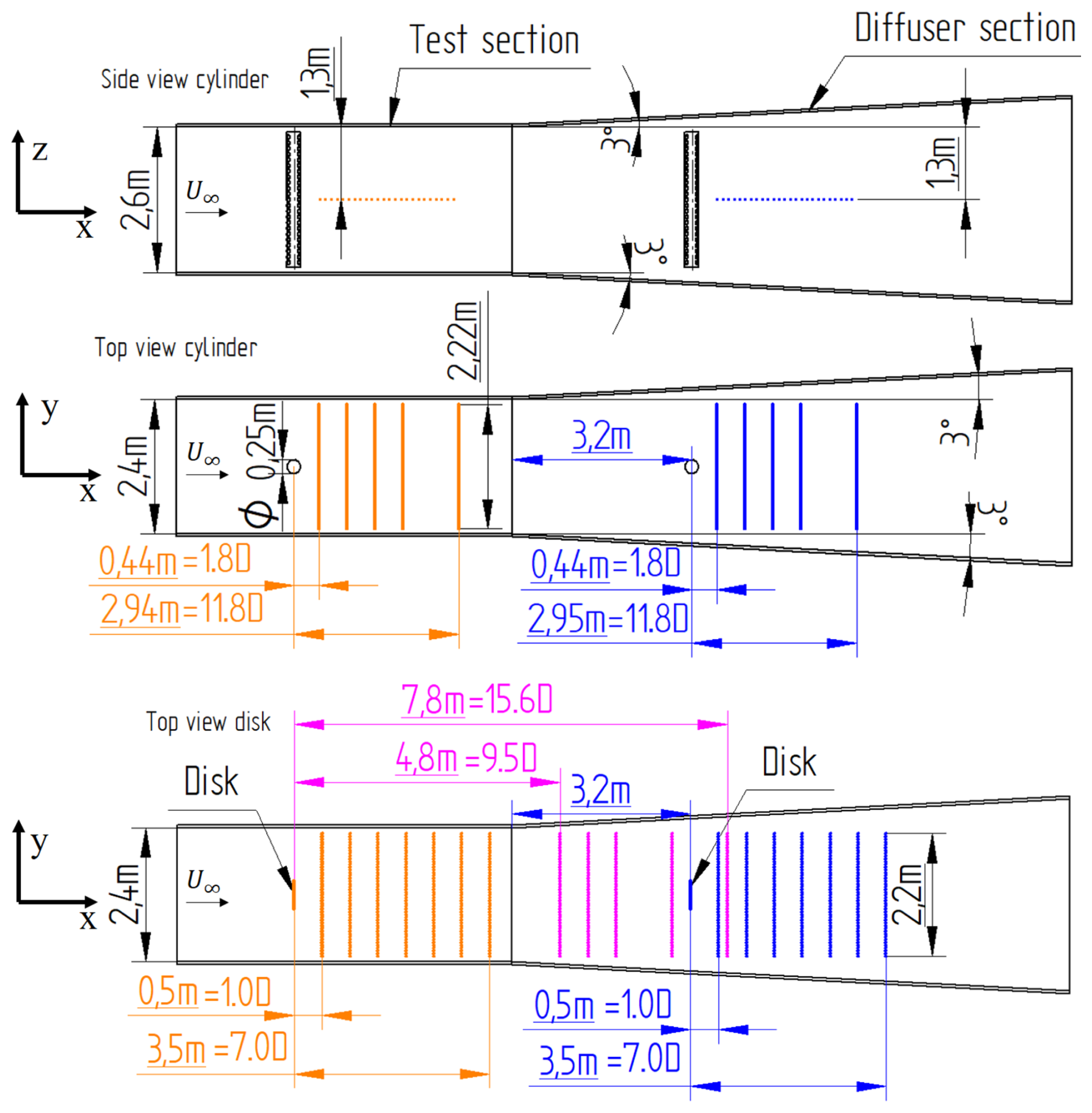
Figure 1 Sketch of the side view of the experimental setup (upper panel) and the top view when the cylinder (middle panel) and the disc (lower panel) are installed. The test section has a length L_TS of 6 m. The wake generator positions were either at the inlet of the test section or at L_DS=3.2 m, which is downstream of the beginning of the diffuser section. A rake of pressure tubes allowed us to create profiles in the central plane of the generator, exploring the x−y plane.

A total of 15 pitot tubes were positioned on a horizontal rack, with a single static pressure probe providing the static pressure. This static pressure probe was positioned in the centre of the rack and slightly above it. The 16 pressure channels were calibrated and recorded with a DTC Initium pressure scanning system at a frequency of 1 kHz. The resolution in terms of pressure of the system is 0.05 %. This implies an absolute error of 0.025 % for the smallest velocity recorded. Nevertheless, given other sources of error in the velocity measurement (such as the calibration of the pressure system), we estimate an absolute error of velocity measurements at 1 %. The minimum duration of each measurement was 60 s, allowing us to resolve and converge the average and rms values of the velocity. As only the averaged and standard deviation values of the signal were extracted, no filter was applied to the raw data. In some cases, very near the generator, the recorded pressure was negative due to the flow reversal in the recirculation region downstream of the disc and the cylinder. In such cases (see for instance Fig. 5a), the recorded velocity was not taken into account in calculations.

The spatial separation of these 15 pressure tubes on the rack was fixed at 15 cm, but the final resolution was increased by offsetting the rack transversely in successive measurements. This meant that for each downstream position, 3×15 positions with 5 cm spacing for the disc and 5×15 positions with a 3 cm resolution for the cylinder were recorded. The measurements also span up to 10 and 9 cm close to both side walls (in the normal section) for the disc and the cylinder, respectively. In the diffuser section, the closest distance to the walls recorded ranges from 29 to 47 cm for the disc and from 28 to 44 cm for the cylinder. The error in the position is estimated as 2 mm. An overview of all measurement stations can be seen in Table 1.

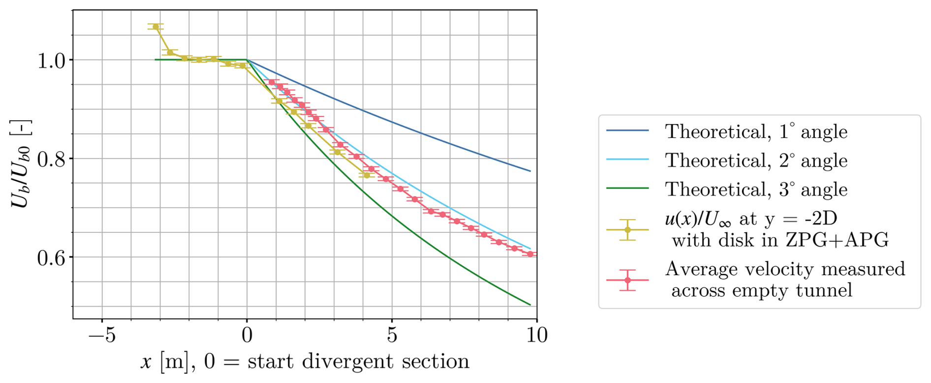
Figure 2 Normalized baseline velocity within the test and diffuser sections for an empty wind tunnel (pink line) and for the disc at $y=-\mathrm{2}D$ (yellow line). The latter is a lateral position that lies outside of the wake throughout all the experimental conditions tested. The figures are compared to the variation in velocity expected from different expansion angles of the walls, deduced via flow rate conservation.

Table 1 Overview of the streamwise distances measured with the rake of pressure tubes, including tests performed for the cylinder and the disc in the test section (TS), diffuser section (DS), and both sections (TS + DS). The sign × implies that no tests were carried out for those conditions. The lateral increment (i.e. the spatial resolution of acquired lateral profiles) is also given.

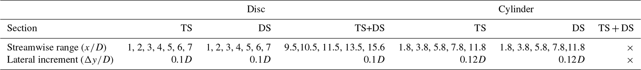
Figure 2 shows the evolution of the averaged streamwise velocity for an empty test section and the evolution of the velocity measured outside the wake. It is observed that the velocity within the diffuser is consistent with a 2^∘ uniform expansion, slightly different from the geometrical expansion of the walls, as governed by Eqs. (10) and (11). This may be due to the development of boundary layers at the walls, and we therefore consider that the APG in our flow is caused by the 2° we observe experimentally. When the disc is present, a small acceleration is also noted very near the generator, caused by the blockage effect of the cylinder.

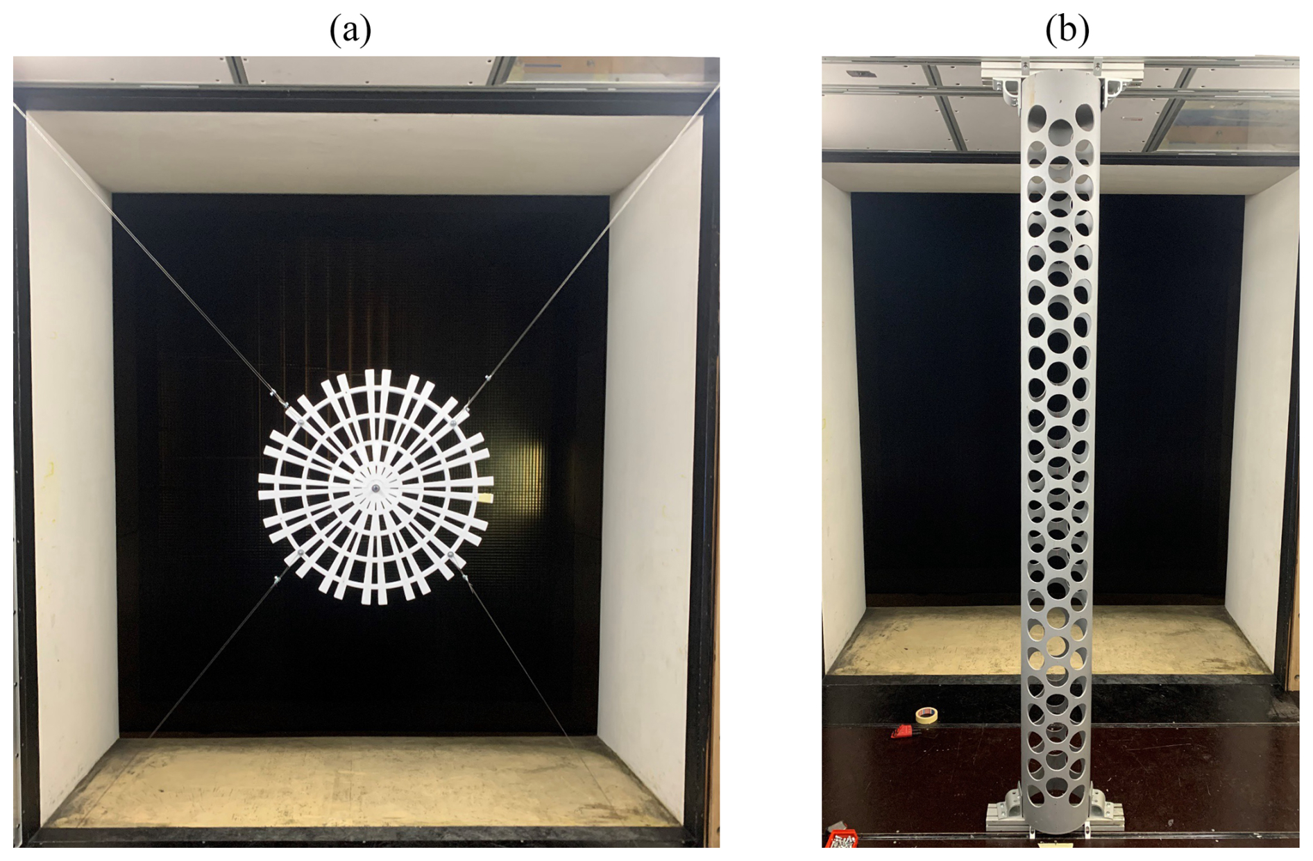
Figure 3 Porous disc (a) and porous cylinder (b) installed at the inlet of the test section, as used in part of this study. The diameters of the disc and the cylinder are 0.5 and 0.25 m, respectively.

Two wake generators were tested, a porous circular cylinder and a porous plate (see Fig. 3), designed in such a way that they had matching drag coefficients. All measurements were made for three different freestream velocities (and therefore different Re_D), and profiles cover several streamwise distances. As stated previously, they were also made by placing the generator either in the test or in the diffusing section. For the latter, the generator was placed 3.2 m downstream after the beginning of the diffuser. For the former, it was placed almost at the inlet of the test section. In the following, we detail the set of measurements performed for each wake generator.

3.1 Porous disc

The disc is made according to the design proposed by Neunaber et al. (2021), which presents a diminishing blockage with the distance from the plate's centre. It has been manufactured in plastic and has a diameter of D=0.5 m, which results in a blockage of 3 %. The disc was held at the centre of the section using 0.75 mm piano wires. The thrust coefficient of the plate is C_T≈0.9, and the porosity is 47 % (the coefficient C_T was not measured here, and the value reported by Neunaber et al., 2021, was used instead).

Measurements include three different freestream velocities, U_∞=7.8, 9.2, and 11.7 m s⁻¹, which correspond to values of Reynolds numbers of ${\mathit{Re}}_D=\mathrm{2.6}\times {\mathrm{10}}^{\mathrm{5}}$, 3.1×10⁵, and 3.9×10⁵, respectively. Horizontal profiles (i.e. in the y direction), for the disc placed either in the test or in the diffuser section, were taken at the same distances with respect to both sections, being approximately $x/D=\mathrm{1}$, 2, 3, 4, 5, 6, and 7 (see Table 1 for the exact values).

For the porous disc an extra profile was measured, where the plate was placed at the entrance of the test section and measurements were done at the diffuser, therefore adding the streamwise distances (all within the diffuser section) of $x/D=\mathrm{9.5}$, 10.5, 11.5, 13.5, and 15.6.

3.2 Porous cylinder

The cylinder has a diameter D=0.25 m, spans vertically the whole section, and is fixated to the floor and the ceiling. It is made of PVC and has 136 circular holes with a diameter of 74 mm, resulting in a porosity, relative to the frontal area, of 43.5 %. It was made following a previous study design (Steiros et al., 2020), which reports a thrust coefficient C_T≈0.9 (matching the value of the disc). The total blockage of the cylinder is 6 %.

The generator was tested at three different streamwise velocities, U_∞=15.6, 18.4, and 23.5 m s⁻¹, which correspond to values of Re_D that match the ones for the disc. Horizontal profiles in the test section were taken at approximately $x/D=\mathrm{2}$, 4, 6, 8, and 12 (see Table 1 for the exact values). When the plate was placed at the diffuser section, the same streamwise distances were recorded.

4 Results

In this section we discuss the effect of the pressure gradient on the velocity deficit and the wake width for both tested objects, as well as the self-similarity of the wake and the effect of the Reynolds number. First, we discuss the raw statistics deduced from our measurements, and we show that, in the conditions studied here, the flow can be considered self-similar (Sect. 4.1). Later, in Sect. 4.2, we discuss the validity of the assumption of the invariability of λ₀ to the pressure gradient. In Sect. 4.3, we focus on the differences in terms of the velocity deficit and wake width between both generators and the presence or absence of an APG. Moreover, we assess if the turbulent wakes still present Reynolds number effects (Sect. 4.4). This analysis is further used in Sect. 5 to apply and discuss the models available in the literature to quantify the effect of an APG.

4.1 Velocity deficit, wake width, and self-similarity

We start this section by discussing the averaged velocity profiles obtained for all conditions tested. Figure 4 shows the normalized averaged streamwise velocity $u/U_{\mathrm{\infty }}$ obtained for different values of x and y. From this velocity contour plot (Fig. 4), it is already clear that the wake evolves differently when it is subject to an APG; in the presence of the APG, both the velocity deficit and the wake width increase.

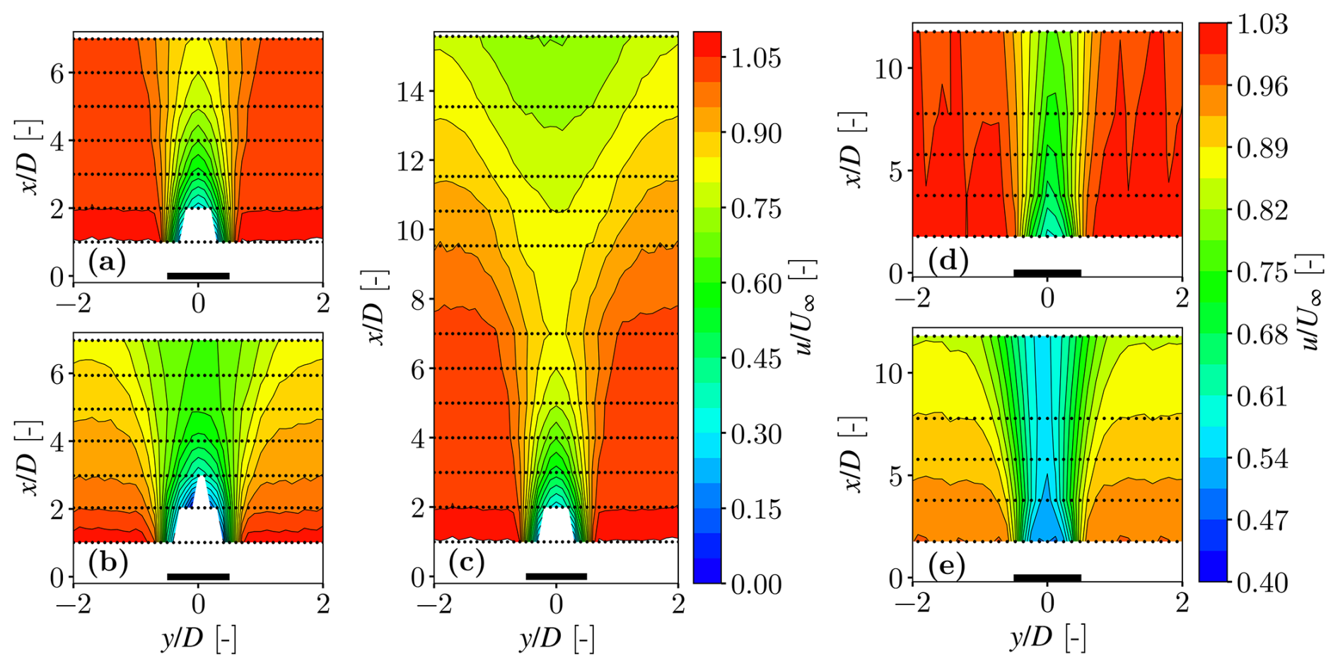
Figure 4 Horizontal profiles of the normalized averaged streamwise velocity $\stackrel{\mathrm{‾}}{u}/U_{\mathrm{\infty }}$ obtained for all cases studies: disc placed in the test section (a), the diffuser section (b), and the test section but expanding through this section and the diffuser one (c). The panel also includes the cylinder placed in the test (d) and in the diffuser (e) section. The black dots represent the points where measurements were taken, and the solid black lines represent the velocity contours. Data were interpolated to generate a map where, in order to better show the details of each wake, the colour scale among panels is not identical.

.

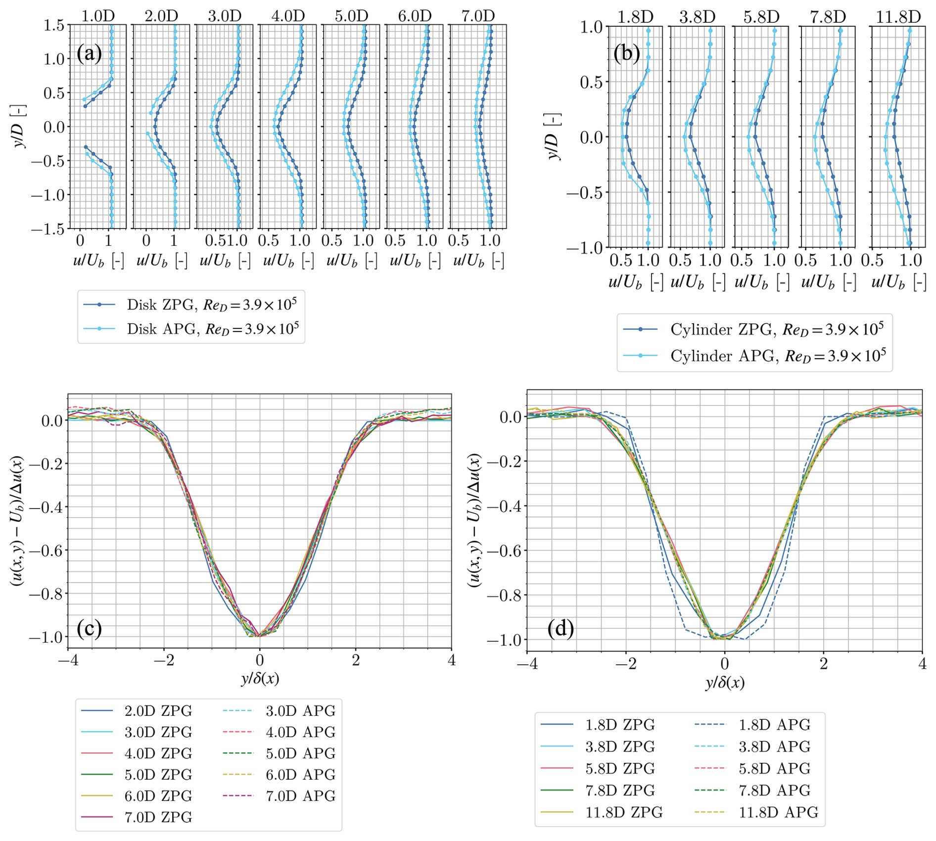
Figure 5 Horizontal velocity profiles of $\stackrel{\mathrm{‾}}{u}/U_{\mathrm{b}}$ in the wake of the disc (a) and the cylinder (b) at different streamwise positions $x/D$ downstream of the generators. The same profiles but normalized using the centreline velocity deficit Δu(x) and the wake width δ (c and d for the disc and the cylinder, respectively). All figures correspond to ${\mathit{Re}}_D\sim \mathrm{3.9}\times {\mathrm{10}}^{\mathrm{5}}$. For panels (a) and (b), the error bars are smaller than the marker size. Panels (c) and (d) aim at showing a qualitative collapse, and therefore no error bars are added

While this difference is obvious when normalizing with the constant U_∞, it is also clear that the wake evolves differently if one normalizes with the velocity U_b(x) (i.e. a decreasing function for increasing x), as shown in the velocity profiles of Fig. 5a and b. Relatively to the ZPG case, the velocity deficit and wake width are both increased.

This can also be seen in Fig. 6a and b, which show the evolution of the velocity deficit and wake width, respectively, of the wakes behind the disc and cylinder at ${\mathit{Re}}_D=\mathrm{3.9}\times {\mathrm{10}}^{\mathrm{5}}$. The velocity deficit seems to evolve with the same slope, regardless of the pressure gradient. Nevertheless, this cannot be said about the wake width, which appears to be strongly affected by the APG. This is not an unexpected behaviour, as the velocity deficit and wake width are related (also shown through Eq. (4): λ(x)∼λ₀(x) for the self-similar streamwise range $x/D\ge \mathrm{3}$; see discussion below). We verified that, regardless of the pressure gradient, the ratio of the velocity deficit and wake width is the same for both the ZPG and the APG, having only a dependency on x.

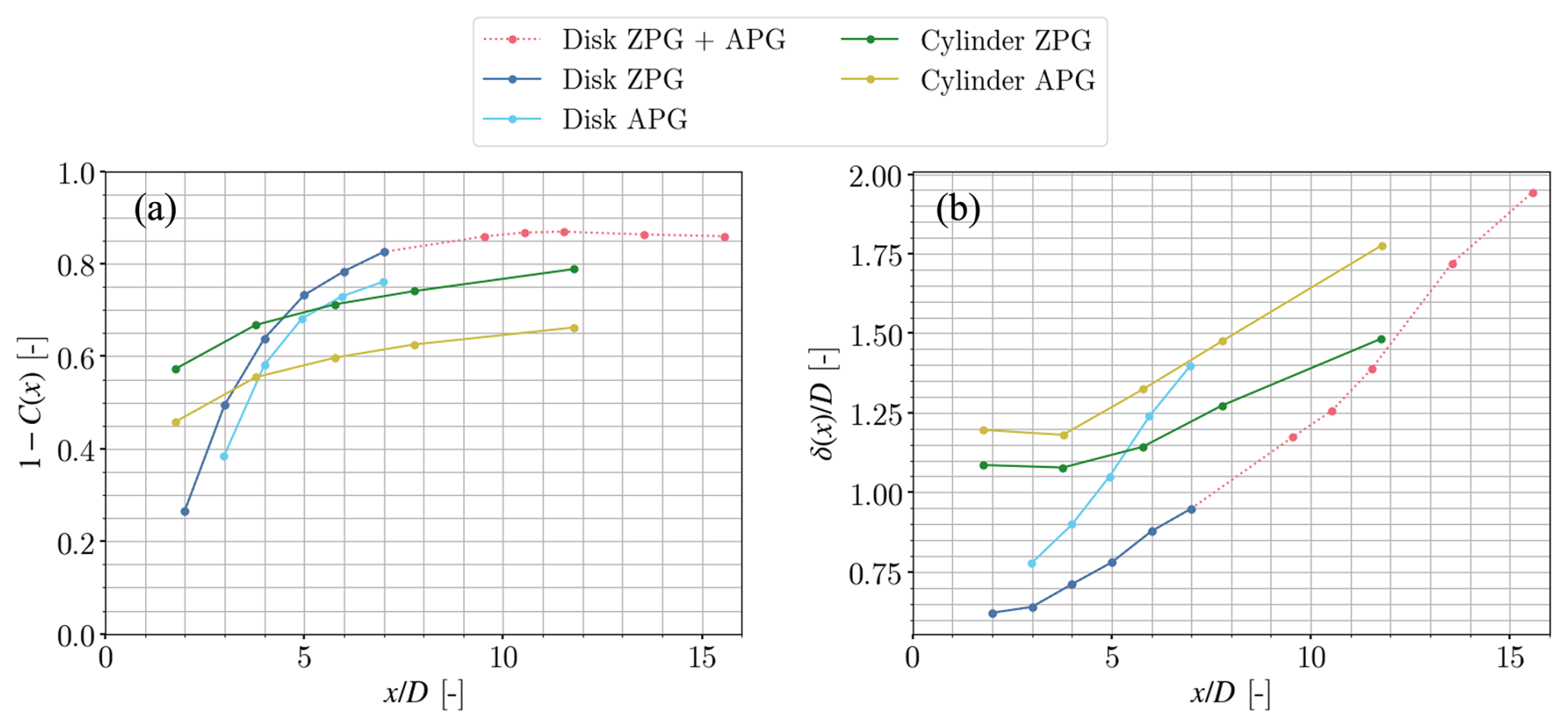
Figure 6 Velocity deficit (displayed as 1−C(x)) (a) and wake width δ(x) (b) for all generators and pressure gradients at ${\mathit{Re}}_D=\mathrm{3.9}\times {\mathrm{10}}^{\mathrm{5}}$.

Furthermore, for both the disc and the cylinder, it can be noted that the profiles $\frac{U_{\mathrm{b}}\left(x\right)-\stackrel{\mathrm{‾}}{u}\left(x,r\right)}{\mathrm{\Delta }u\left(x\right)}$ collapse when the radial distance is normalized with the wake width δ(x) (Fig. 5c and d). In all cases, δ is estimated as the standard deviation of a Gaussian fit applied to the velocity profile $U_{\mathrm{b}}\left(x\right)-\stackrel{\mathrm{‾}}{u}\left(x,r\right)$ at a given x position. Δu(x) is the maximum velocity deficit at a given x position. It is defined as $\mathrm{\Delta }u\left(x\right)=U_{\mathrm{b}}\left(x\right)-min\left(\stackrel{\mathrm{‾}}{u}\right(x,y\left)\right)$. In consequence, we can conclude that the wake, for all cases studied, in the range $x/D\ge \mathrm{3}$, can be regarded as self-similar (at least in terms of the averaged velocity field).

Finally, it must be noted that the wake of the cylinder is slightly skewed. Our measurements for an empty test and diffuser section show that the baseline velocity in the tunnel is not asymmetric. Therefore, this effect is most likely due to the cylinder positioning. While great care was taken in positioning the cylinder in the tunnel, it is possible that a very small angle was created between the centreline of the holes and the incoming flow, causing a small skewness on the wake.

4.2 Invariability of λ to pressure gradient

As mentioned above, the ratio of the velocity deficit to the wake width, as given by Eq. (4), is a key relation in the model proposed by Shamsoddin and Porté-Agel (2018). In the studies by Liu et al. (2002) and Thomas and Liu (2004), it is shown that λ is invariant to the pressure gradient. This invariance is also depicted in Fig. 7 for the disc and cylinder at ${\mathit{Re}}_D=\mathrm{3.9}\times {\mathrm{10}}^{\mathrm{5}}$. From this figure, it can be observed that the evolution of this parameter in the streamwise direction in the wake of either wake generator follows a very similar pattern, regardless of the pressure gradient. Therefore, using this invariability to solve the ODEs in Eqs. (2) and (9) appears to be a valid assumption.

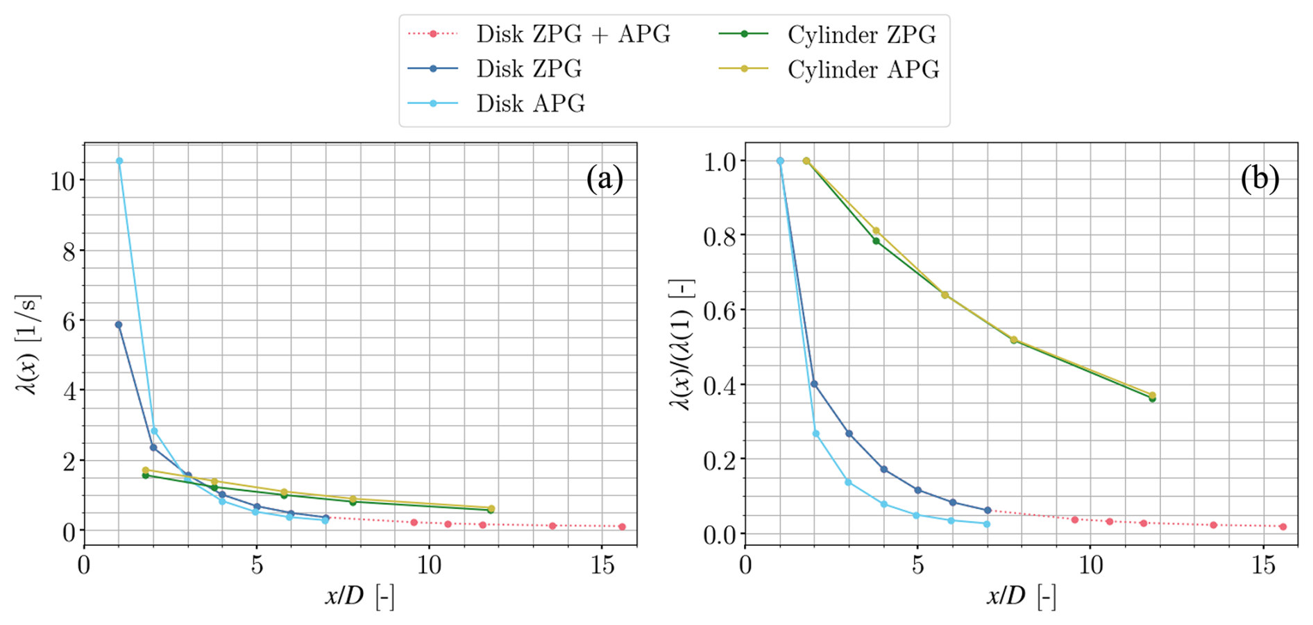
Figure 7 Streamwise dependence of the ratio $\mathit{\lambda }\left(x\right)=U_{\mathrm{b}}\left(x\right)C\left(x\right)/\mathit{\delta }\left(x\right)$ (Eq. 4) for all generators at ${\mathit{Re}}_D=\mathrm{3.9}\times {\mathrm{10}}^{\mathrm{5}}$. Panel (a) shows the absolute value, while panel (b) normalizes it to λ(x) at x=1D.

However, there is an offset in the absolute value between the ZPG and APG cases. This offset is not shown in the studies by Liu et al. (2002) and Thomas and Liu (2004), as their work scales the value of λ(x) relative to λ(0) at x=0. A similar scaling has been applied to Fig. 7a, shown in Fig. 7b, such that λ(x) is scaled to the first measured value. In the case of the cylinder, the two curves collapse. In the case of the disc, there is a small absolute offset between the ZPG and APG cases. In the far wake the curves seem to reach the same asymptote. Scaling it to the first value does not seem to work well because the near wake is difficult to characterize due to the negative velocities encountered close to the disc. Thomas and Liu (2004) note that differences in the absolute value may arise due to differences in the Reynolds numbers. It appears that small differences between the experimental setups for the ZPG and APG cases have resulted in this small difference in the absolute value of λ(x). Unfortunately, this offset remains relatively constant, causing a relative difference of 20 %–30 % between the two cases at larger values of $x/D$. As is shown in Sect. 5, variations in λ(x) result in only minor errors in the calculated velocity deficit. However, since the calculation of wake width in the model by Shamsoddin and Porté-Agel (2018) is directly proportional to the absolute value of λ₀, any uncertainty in this parameter directly translates to the same level of uncertainty in the estimated wake width. This means that the 20 %–30 % relative difference is also present in the wake width. Thus, while the invariability of λ(x) to the pressure gradient is confirmed, it is critical to measure its absolute value accurately, especially in the near wake.

4.3 Differences between disc and cylinder

Remarkably, the effect of the APG is significantly different for the two different generators. For instance, for the disc, the value of 1−C(x) is approximately 7 %–9 % smaller for the APG with respect to the ZPG, while the wake width δ is larger, with a difference ranging from 21 % at x=3D to 47 % at x=7D (Fig. 6a and b). On the other hand, the differences for the cylinder are 16 %–20 % for 1−C(x) and range from 10 % to 20 % for δ.

From the velocity profiles in Fig. 5a and b, it can be observed that for the disc, very near the generator (x=1D to x=2D), the velocity becomes negative. The profiles are incomplete, as the pitot tubes cannot measure these negative velocities. This is not the case for the cylinder: even if the C_T of both objects was designed to be the same, the near wakes generated by these two objects differ significantly. This can be attributed to the fact that the wake of the cylinder is two-dimensional, while the disc has a three-dimensional wake. It is not unexpected that a two-dimensional case has a stronger wake.

Finally, the velocity profiles in the wake of the cylinder do show two other significant differences between the ZPG and APG case. First of all at x=2D, the wake in the APG is not yet Gaussian. It appears it takes a slightly longer distance for the velocity profiles, as shown in Fig. 5d, to collapse as compared to the disc. Second, the wake of the cylinder in the APG case is slightly skewed towards negative values of y.

4.4 Effect of Reynolds number

Figure 8a–d show the streamwise evolution of the centreline velocity deficit (displayed as 1−C(x)) and δ(x) for the three values of Re_D considered in this work. First, the effect of the APG is the same for all Reynolds numbers and generators, increasing the velocity deficit C(x) and increasing the wake width δ(x). Furthermore, it can be observed that, for the disc, all curves collapse (Fig. 8a and b) onto a single curve, showing low sensitivity to Reynolds numbers. The cylinder, displayed in Fig. 8c–d, shows a similar behaviour for the two larger Re_D values. However, the smallest Reynolds number (${\mathit{Re}}_D=\mathrm{2.6}\times {\mathrm{10}}^{\mathrm{5}}$) presents some deviations with respect to the other curves. Identical trends are observed when checking the Reynolds number dependence for the horizontal profiles of the velocity deficit (such as the ones displayed in Fig. 5, not shown here for the other values of Re_D). We therefore conclude that for all generators, results become independent of Re_D for the two largest values tested.

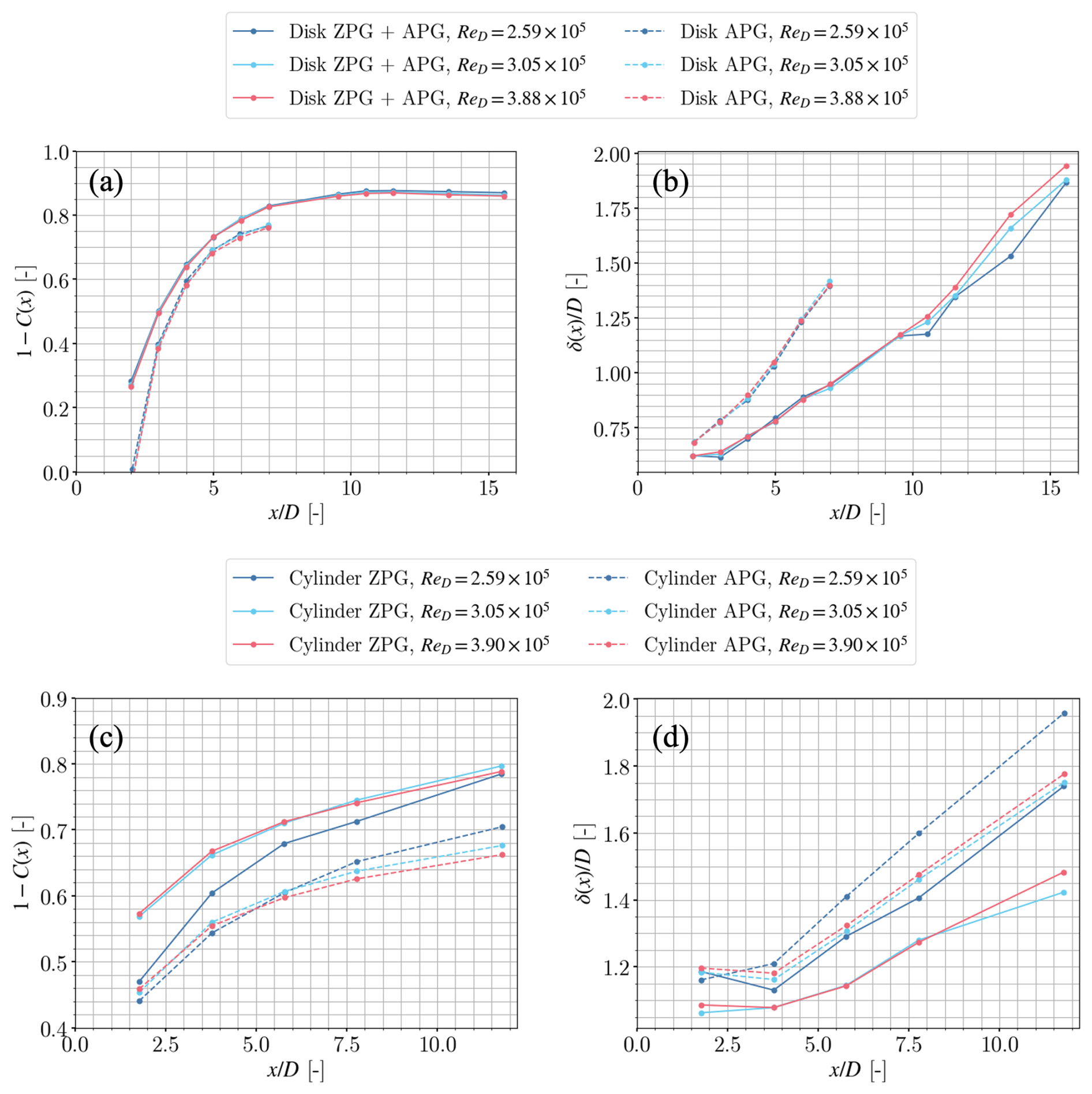
Figure 8 Velocity deficit (displayed as 1−C(x)) and wake width δ(x). Influence of the Reynolds number Re_D on these parameters for the disc (a, b) and the cylinder (c, d).

In the following, we discuss our dataset in terms of the models introduced in Sect. 2. Given the discussion above, we report only results collected at the largest value of the Reynolds number, namely ${\mathit{Re}}_D=\mathrm{3.9}\times {\mathrm{10}}^{\mathrm{5}}$.

5 Comparison with the models from the literature

We now focus on how our dataset can be described by the models discussed in Sect. 2. First, to be able to apply the theory, the turbulent wakes have to be self-similar, an aspect that has already been verified in the last section.

5.1 Porous disc

Figure 9a and b show the results of the model developed by Shamsoddin and Porté-Agel (2018), described in Sect. 2.1. In particular, Fig. 9a shows the model applied to a wake starting in a ZPG that continues into an APG. In order to apply the model, a baseline wake in the ZPG case is needed for the entire range up to x=15.8D as input for the model. Because the length of the test section was limited, no measurements exist after x=7D for the ZPG case. As discussed in Sect. 2.1, to generate the ZPG velocity deficit and wake width for x>7D, a power-law fit was made according to Eqs. (6) and (7). This fit is based on the ZPG case up to x=7D and extrapolated until x=15.8D. The velocity deficit and wake width are simultaneously fitted to the two-dimensional velocity field as a two-dimensional Gaussian fit with a fixed virtual origin. In this Gaussian fit (see also Eq. 1), the simultaneous velocity deficit and wake fits resulted in the following constants: A=1.330, α=1.10, B=0.187, β=0.51, and x₀=0.724. C₀(x) and δ₀(x) are then used to calculate λ₀ in Eq. (4). Then, Eq. (2) can be solved, obtaining the streamwise scaling of C(x).

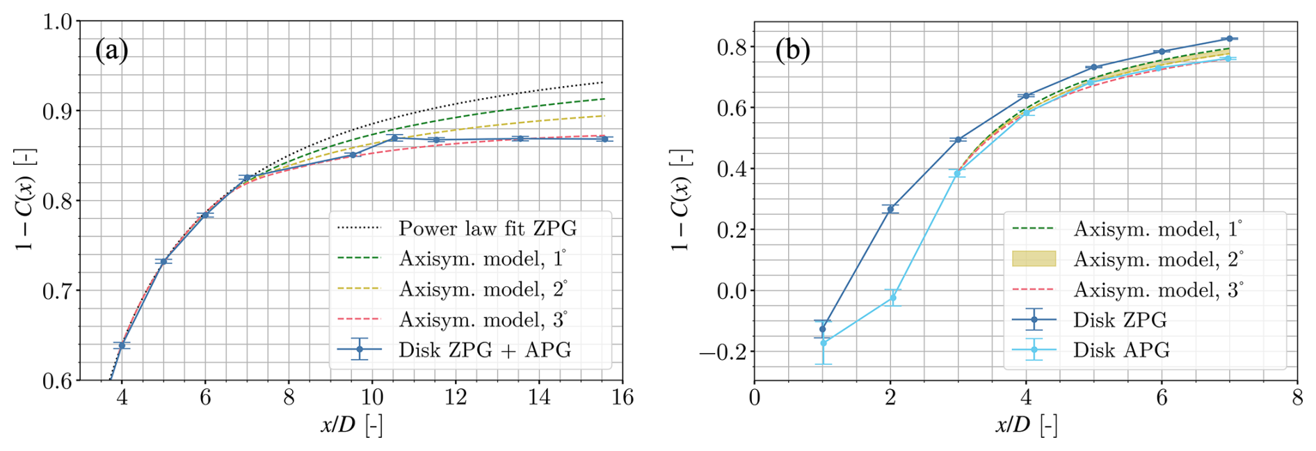
Figure 9 (a) Velocity deficit 1−C(x) in the wake of the disc with a ZPG continuing into an APG. A power-law fit shows how the wake is expected to evolve if there had been no pressure gradient after x=7D. (b) ZPG experimental results versus APG experimental results of the wake behind the disc. Model output with input from the ZPG case is shown for three different wall angles. The shaded area shows the difference between using λ₀ and λ_APG as input.

The model fits both cases considered in our experimental setup remarkably well, with the first case being the APG following a ZPG (i.e. the disc placed at the inlet of the test section and the turbulent wake evolving freely across the test section and into the diffuser, Fig. 9a). The model also properly describes the turbulent wake fully immersed in the APG (i.e. the generator installed in the diffuser, Fig. 9b). Moreover, while both possible expansions of the diffuser section work (i.e. 2 or 3°), the best fit is found for 3°. This is not fully consistent with the effective expansion found in Fig. 2 for an empty test section, yet it fits with the actual geometric expansion of the wind tunnel. Nevertheless, by only giving a starting point of C(x_i) and the ZPG wake, the model is able to predict the evolution of the velocity deficit in the wake in an APG extremely well. Small differences in terms of the expansion angle that fits the generators may also be related to blockage effects and differences in the boundary layer development at the walls in the presence of the wake generators.

The main difference between both situations considered is that when the wake fully develops in the test section, the model can only be applied downstream of the near wake, which in our case is $x/D\ge \mathrm{3}$. On the other hand, the model by Shamsoddin and Porté-Agel (2018) properly matches the transition of the wake from the ZPG to the APG. This is a reasonable expectation, as the model has been developed to describe the far-wake behaviour, where the transverse profiles are Gaussian (or near Gaussian), and the wake is self-similar.

Finally, in the case of the disc, the model is quite sensitive to the input λ₀. This becomes clear from Fig. 11a, where large differences are observed between the estimated wake widths. Generally, the model is unable to predict the actual wake width, unless the λ_APG is used. λ₀ and λ_APG should be the same, but a small difference, as observed in Fig. 7, results in a large difference in the wake width.

5.2 Porous cylinder

Comparing the evolution of the velocity deficit and wake width in the wakes of the cylinder and the disc in Fig. 6, one can see that the velocity deficit and wake width evolve differently for the wakes of the disc and cylinder. This supports the requirement of using the different ODE of Eq. (9) for the cylinder. Other than this feature, the porous cylinder presents a similar behaviour to the one described for the axisymmetric wake in the previous section.

As shown in Fig. 10, the streamwise evolution of the wake in the APG is very well modelled by Eq. (9). Nevertheless, whether this behaviour still holds further downstream (x>12D) remains an open question. In this case, an effective expansion between 1 and 2° works well as an input to the model. Furthermore, unlike the disc, the wake width is predicted well with the assumption of λ₀, as shown in Fig. 11b. The fits were still performed according to Eqs. (6) and (7), resulting in A=0.71, α=0.47, B=0.15, β=0.35, and $x_{\mathrm{0}}=-\mathrm{1.01}$. We remark that unlike for the disc, given the limitations of the experimental setup, for the cylinder the case where the cylinder is placed in the ZPG and the wake evolves from the ZPG into an APG has not been considered.

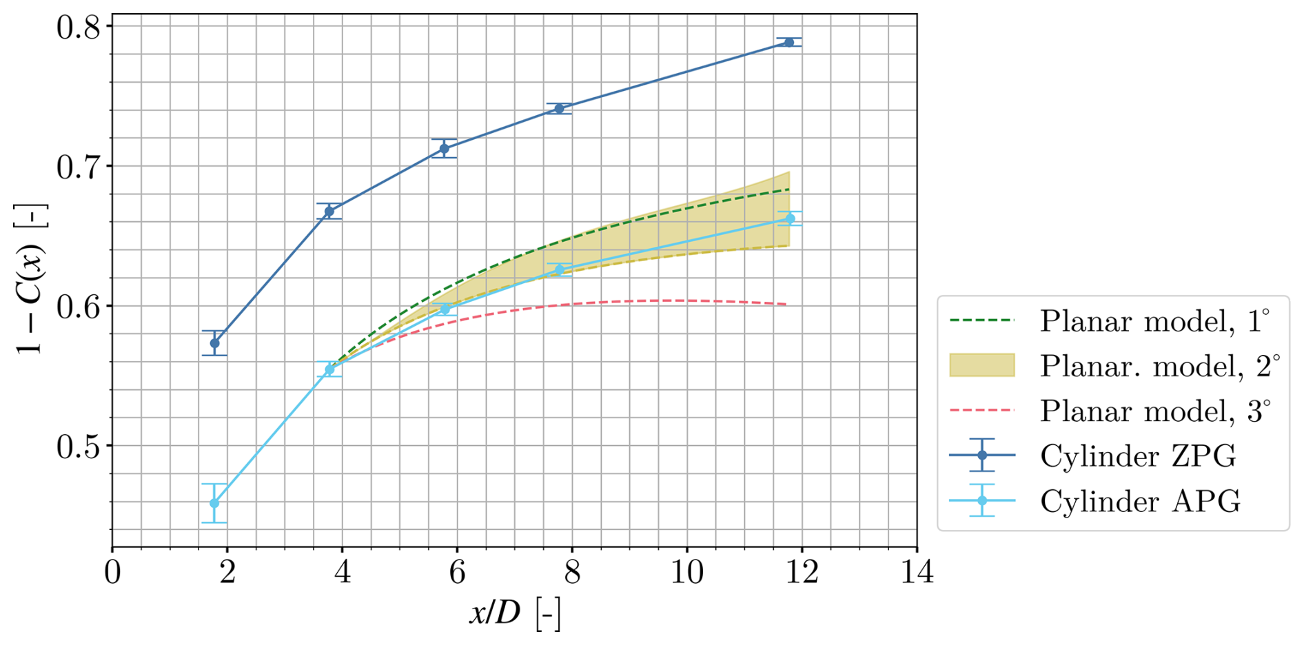
Figure 10 ZPG experimental results versus APG experimental results of the wake behind the cylinder. Model output with input from the ZPG case is shown for two different wall angles. The shaded area shows the difference between using λ₀ and λ_APG as input.

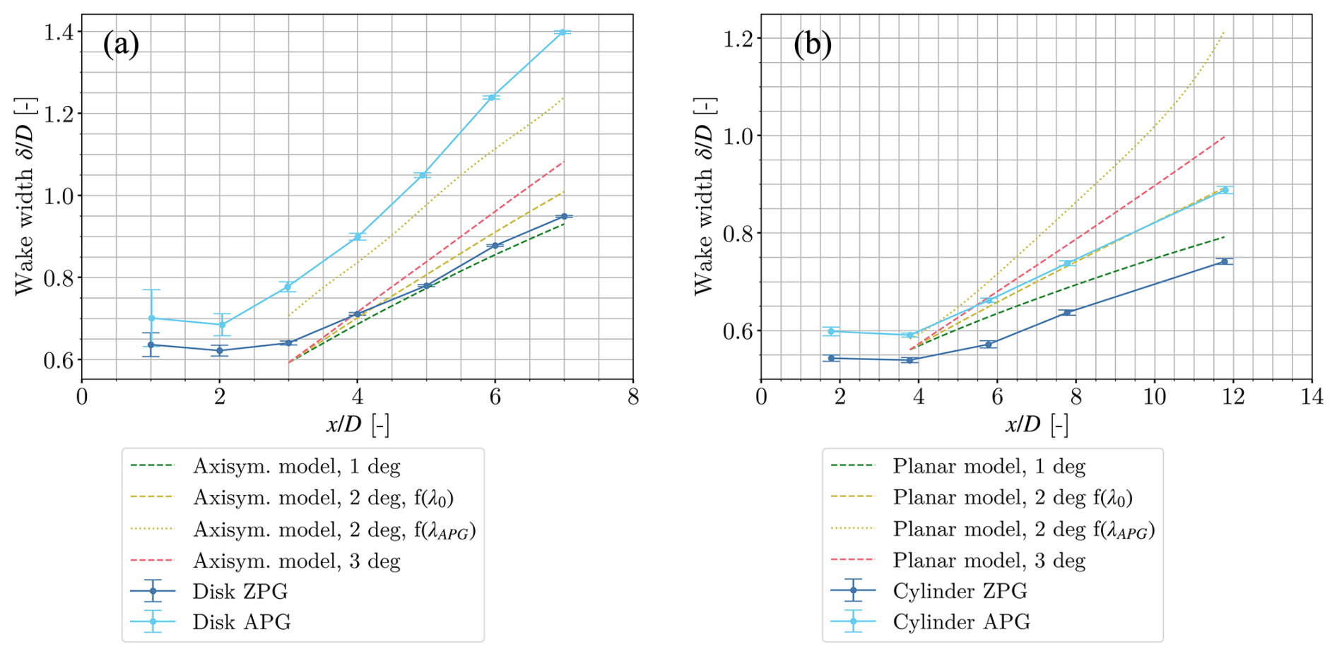
Figure 11 ZPG experimental results versus APG experimental results of the wake width of the wake behind the disc and cylinder. Model output with input from the ZPG case is shown for three different wall angles and a different λ. (a) Disc. (b) Cylinder.

To conclude this section, excellent agreement between our experimental dataset and the analytical models by Shamsoddin and Porté-Agel (2017) and Shamsoddin and Porté-Agel (2018) has been found for all experimental conditions tested. While our experimental setup is limited in terms of temporal resolution, further studies using hot-wire anemometry and/or particle image velocimetry could help to evaluate further statistics within an adverse pressure gradient. For instance, they would allow us to validate some hypotheses from the models, particularly regarding the self-similarity and axisymmetry of all relevant terms of the kinetic energy and momentum budgets.

6 Conclusions

In this work, we developed an experimental setup specially adapted to assess the influence of an adverse pressure gradient in a wind tunnel. Using the properties of the ISAE-ENSMA wind tunnel in Poitiers, the spatial evolution of a turbulent wake was characterized under conditions of either no pressure gradient or an adverse one. A streamwise range of distances pertinent to wind energy applications was evaluated (2 to 12 diameters) for a porous disc and a cylinder, which are known to be representative of horizontal- and vertical-axis wind turbines, respectively.

We found that the pressure gradient has a strong effect on the wake profile, centreline velocity deficit, and wake width for both families of generators. This effect is also different for the wake generated by a cylinder or a disc. Another significant difference is that, within the range of Reynolds numbers studied (2.6×10⁵ to 3.9×10⁵), the disc presents no Reynolds number effects, while the cylinder wake only becomes independent of this parameter for ${\mathit{Re}}_D>\mathrm{2.6}\times {\mathrm{10}}^{\mathrm{5}}$. Moreover, the lateral profile of the velocity deficit of the turbulent wake for both generators is properly modelled by a Gaussian curve for downstream distances larger than 4 diameters.

Within a regime that is independent of the Reynolds number based on the generator diameter, the centreline velocity deficit and wake width are significantly increased in the presence of such a gradient. This is verified for wakes that fully evolve within a pressure gradient (i.e. with the generator placed within it) or that develop through a zero-pressure gradient section followed downstream by an adverse one. Moreover, the analytical models developed by Shamsoddin and Porté-Agel (2017, 2018), based on averaged momentum conservation, properly match all of our experimental datasets.

These experiments are in good qualitative agreement with similar works on pressure gradients. The main novelty lies in the simultaneous study and comparison of planar and axisymmetric wakes within the same facility at relatively large values of turbulent Reynolds numbers. While most studies focus on averaged large-scale quantities, such as the velocity deficit and wake width, our experimental setup can also be repurposed to study small-scale turbulence quantities, such as intermittency, dissipation, and spectral dynamics. Such studies would contribute to the development of closures for theoretical and numerical models of wind-turbine- and water-turbine-generated wakes.