Efficient derivative computation for unsteady fatigue-constrained nonlinear aero-structural wind turbine blade optimization

Gradient-based optimization offers significant efficiency advantages for wind turbine blade design, but its application has often been limited by the cost and accuracy of finite-difference derivative calculations, especially when fatigue constraints are considered. In this work, we systematically compare and evaluate four differentiation techniques, namely algorithmic differentiation, implicit differentiation, sparsity exploitation, and parallelization, to determine their effectiveness in computing accurate gradients through time-domain aero-structural simulations. By integrating these techniques with unsteady nonlinear aerodynamic and structural models, we develop software designed for accurate gradient computation. We show that combining these techniques addresses memory and runtime challenges associated with long simulations required by design load cases. Specifically, the most effective combination reduces derivative computation wall time by over an order of magnitude compared to finite differencing while maintaining superior accuracy. We demonstrate this approach in a proof-of-concept aero-structural optimization of a wind turbine blade that improves the cost of energy by 12.78 %. This comparative study establishes a viable approach for fatigue-aware blade design that balances computational efficiency with modeling accuracy.

1 Introduction

Designing a cost-effective wind turbine blade is a difficult task for many reasons, but one salient challenge is including the large number of variables required to fully specify a design. Gradient-based optimization provides a systematic approach to this problem, as it typically finds optima more efficiently than gradient-free methods for design problems with many variables (Ning and Petch, 2016). Gradient-based optimization adds the additional challenge of obtaining the derivatives of the objective and constraints with respect to the design variables.

This challenge can be broken into two main categories: (1) derivative accuracy and (2) derivative computation time. Traditionally, derivatives have been calculated using finite-difference methods, which are limited in both accuracy and computation time. Despite the challenges, many have done excellent work in this field using finite differences. Døssing et al. (2012), Kwon et al. (2015), and Frontin et al. (2023) completed aerodynamic-only blade optimizations. Several studies have used traditional forms of finite differencing to complete aero-structural optimization (Bottasso et al., 2016; Zahle et al., 2016; Pavese et al., 2017; Bortolotti et al., 2018; McWilliam et al., 2018b, a; Ingersoll, 2020; Scott et al., 2022; Serafeim et al., 2022). Kenway and Martins (2008) and Madsen et al. (2022) used a complex-step finite-difference method.¹

Algorithmic differentiation (AD) provides a powerful alternative to finite-difference methods that directly addresses the challenges of gradient-based optimization. AD computes the derivatives of the individual operations of an analysis software. Iterative application of the chain rule propagates these derivatives through the code. This approach provides the desired derivatives of function outputs (Naumann, 2011). The main added cost of using AD is that the value of the derivative and tracking information must be stored, which results in increased memory requirements. AD approaches have already been included in several works, such as Ning and Petch (2016), Dhert et al. (2017), and Allen et al. (2020).

The computational cost of AD increases substantially when propagated through iterative solvers. Implicit differentiation methods offer an attractive solution by analytically computing derivatives of equations solved iteratively, bypassing the need to differentiate through the solver itself. Several studies have successfully applied implicit differentiation approaches (Dhert et al., 2017; Madsen et al., 2019; Batay et al., 2023; Mangano et al., 2025; Hermansen et al., 2025). However, manual implementation of implicit differentiation is often cumbersome and problem-specific. In previous work, we demonstrated how implicit differentiation can be automated by applying AD to converged solver residuals, enabling efficient derivative computation with minimal implementation effort for AD-compatible solvers (Ning and McDonnell, 2023).

Derivative computation can be made more efficient by taking advantage of two key properties: sparsity and parallelization. In many engineering problems, Jacobians are sparse, meaning that many of the entries in the Jacobian are zero. By identifying and leveraging this sparsity structure, techniques such as graph coloring can substantially reduce the number of derivative computations required. In previous work, we demonstrated how exploiting sparsity reduced the derivative computation cost in a steady aerodynamic optimization problem (Ning, 2021) and in wind farm layout optimization (Varela and Ning, 2023). Complementing this approach, parallelizing the derivative computations across multiple processors can further decrease the wall time required.

The design of a cost-effective wind turbine blade is inherently an aero-structural problem (Bottasso et al., 2016). One critical aspect of wind turbine design is accounting for the effects of fatigue in the design. Several different approaches have been used to include fatigue in the design, such as iterative methods (Bottasso et al., 2016; Bortolotti et al., 2018; Ingersoll, 2020), simplified models (Ning and Petch, 2016), frequency-domain approaches (Pavese et al., 2017), and precomputing fatigue loads and scaling them by the static stress (Hermansen et al., 2025). Although these approaches have been successful, they do not incorporate fatigue calculations based on the unsteady loads of the current design directly into the optimization loop. As a result, the optimization algorithm cannot fully explore the design space and often creates over-engineered designs.

While fatigue has been incorporated into wind turbine optimization through various approximations, Scott et al. (2022) directly compute fatigue damage from time-series simulations within the optimization loop. Their approach evaluates unsteady loading histories, applies the rainflow counting algorithm, and calculates fatigue damage explicitly rather than relying on surrogate models or approximations. This approach, however, depends on simplified modeling assumptions. Specifically, they employed a linearized aerodynamic model coupled with a modal beam model that neglects geometric nonlinearities. As with other linearized models, this formulation loses accuracy when evaluated away from the linearization point. Scott et al. (2022) report that this leads to overpredicted axial and torsional deflections, reduced aero-elastic damping, and inflated estimates of flapwise damage equivalent loads.

Analyzing fatigue in the optimization loop significantly increases the difficulties already presented by gradient-based optimization. The foremost challenge is obtaining accurate gradients through time. Time-domain gradient computation presents significant challenges, as Zahle et al. (2016) observed when computing finite-difference derivatives of tip-tower clearance. More recent work (Scott et al., 2022; Frontin et al., 2023) has shown ways to improve the accuracy of unsteady gradients. In addition to using more accurate differentiation techniques, tight convergence of the aerodynamic and structural states can improve accurate gradient computation. A secondary challenge that arises is the length of time-domain analyses required to compute fatigue loads. The design load cases (DLCs) require that wind turbine designs account for 600 s of turbulent inflow (International Electrotechnical Commission, 2019). Long simulations not only directly increase the derivative computation time, but also increase the memory requirements of AD. These challenges make the choice of analysis software critical. While higher-fidelity software increases the accuracy of the solution (and thus the gradient), it comes with time and memory requirements that make it intractable to include long enough time-domain simulations to conduct meaningful fatigue analysis in the optimization loop. Furthermore, current mid-fidelity software that would not be limited by time and memory requirements is not compatible with modern derivative computation methods.

We address the challenges of conducting fatigue analysis within the optimization loop by coupling unsteady nonlinear aerodynamic and structural solvers designed for accurate and efficient derivative calculation. To identify the most effective approach, we systematically compare multiple differentiation techniques: forward- and reverse-mode AD, implicit differentiation, parallelized implementations, and sparse formulations. We first introduce the model and its sub-models and then present the various differentiation approaches in the methods section. After describing the optimization problem, we verify the model and compare the computational performance of each differentiation technique before discussing the optimization results.

2 Methods

We first describe the aeroelastic model's coupling strategy and sub-models, establishing the computational structure through which derivatives must be propagated. The subsequent subsections detail our approach to derivative computation, including AD, automated adjoints, parallelization, sparsity exploitation, and constraint aggregation techniques that enable practical gradient-based optimization of this complex system.

2.1 Model overview

Our model architecture draws inspiration from the National Laboratory of the Rockies’ WEIS framework (https://github.com/WISDEM/WEIS, last access: 21 November 2025), which integrates OpenFAST (https://github.com/OpenFAST/openfast, last access: 21 November 2025), PreComp (https://www.nrel.gov/wind/nwtc/precomp, last access: 21 November 2025), and pCrunch (https://github.com/NREL/pCrunch, last access: 21 November 2025). We developed our own implementation rather than adopting these established tools for two key reasons. First, implementing everything in Julia (Bezanson et al., 2017) provides seamless access to automatic differentiation packages with minimal code modification. Julia's just-in-time compilation also delivers computational performance comparable to Fortran or other compiled languages. Second, our structural solver, GXBeam (https://github.com/byuflowlab/GXBeam.jl.git, last access: 3 December 2025), employs constant property linear elements with extended Milenković parameters. This formulation produces an exceptionally robust solver that avoids excessive quadrature, enabling tight convergence of structural states at each time step. Such robust convergence stabilizes the entire coupled aeroelastic solution and proves critical for obtaining accurate gradients through time. This Julia-based implementation is not intended to replace OpenFAST but rather serves as a research platform for rapidly prototyping and evaluating differentiation techniques. Successful approaches demonstrated here could inform future implementation in OpenFAST or similar established software packages.

Figure 1 summarizes the overall model, which may be partitioned into three distinct stages: a precomputation step, a time-domain analysis, and a post-processing step. The core of the time-domain analysis is a two-way coupled, partitioned model that converges across time. It uses blade element momentum theory (BEMT) to predict an angle of attack and an inflow velocity. The model uses the angle of attack and inflow angle to predict time-varying loads via the Beddoes–Leishman dynamic stall model. Geometrically exact beam theory (GEBT) uses those loads to predict the dynamic response of the wind turbine blade. The linear and angular deflections and velocities are used to augment the inflow conditions seen by the BEMT for the next time step. The code of the time-domain analysis is implemented in the package WATT.jl (https://github.com/byuflowlab/WATT.jl.git, last access: 3 December 2025). Verification of the current model is shown in Sect. 3.1.

Figure 1 Flowchart of the coupled wind turbine blade model.

The precompute step uses classical laminate theory (CLT) to calculate the required mass and compliance properties. Also computed before run time is a turbulent wind field using TurbSim (https://www.nrel.gov/wind/nwtc/turbsim, last access: 21 November 2025). The post-process step uses CLT to calculate the strain in each cross-section. Rainflow counting is used to separate the strain signal into load ranges and corresponding counts. Miner's rule is used to linearly accumulate damage. In the following subsections, we discuss each of the sub-models. Sub-models that are not referenced in their own repositories are included in this paper’s companion repository.

2.1.1 Blade element momentum theory

BEMT is well-documented in standard aerodynamic texts (Burton et al., 2011), so here we focus on its application within our aero-structural coupling framework. For our BEMT, we use Ning's (Ning, 2021) one-residual formulation inside of the code package CCBlade.jl (https://github.com/byuflowlab/CCBlade.jl, last access: 3 December 2025). Using a BEMT with one residual allows for solvers with guaranteed convergence such as Brent's method (Brent, 2013). This reliability transfers through to the derivative calculation, providing smooth derivatives of the aerodynamic solution across the design space.

Prandtl tip corrections are applied at both the hub and the tip. The 2D airfoil polars from the wind turbine description (Resor, 2013) are provided at 17 spanwise stations and have been smoothed using B splines. Linear interpolation between these stations produces airfoil polars at each blade node. The smoothing and interpolation are performed as a preprocessing step, while Akima splines (Akima, 1970) interpolate each polar during the solution process.

2.1.2 Dynamic stall model

To enable unsteady analysis with BEMT, we implement the Beddoes–Leishman dynamic stall model incorporating Gonzalez's modifications (Jonkman et al., 2017). Our implementation follows the discrete ordinary differential equation formulation from OpenFAST v3.5.1 and is available in DynamicStallModels.jl (https://github.com/byuflowlab/DynamicStallModels.jl, last access: 3 December 2025). The state predictions match those of OpenFAST to machine precision.

2.1.3 Turbulence model

In the pre-process step (and outside of all optimization loops), we generate a spatially uniform turbulent wind field using TurbSim. The outputs used at every time step of the time-domain analysis are the three components of the wind speed (U, V, and W). For simplicity, the velocity is assumed to be uniform across the rotor plane; however, WATT.jl could be easily extended to accommodate a spatially varying wind field. WATT.jl is already capable of using a temporal discretization independent of the time step used in the turbulence model, but the results are co-located for the purpose of this study.

2.1.4 Geometrically exact beam theory

As previously mentioned, we use the nonlinear GEBT solver GXBeam.jl (McDonnell and Ning, 2024) to predict the structural response of the wind turbine blade. The formulation of GXBeam allows large deflections and rotations, while maintaining solution robustness and derivative stability. GXBeam uses the Newmark-beta method to integrate the equations of motion across time. The inputs to the model are the loads, the blade geometry, and the material properties. The outputs used for the aero-structural coupling are the linear/angular deflections and velocities. The internal forces and moments are also available for post-processing. The blade is modeled as a cantilevered beam with a fixed root and free tip. Aerodynamic loads are rotated into the root reference frame and applied as non-following distributed loads, which are assumed constant across each element.

2.1.5 Classical laminate theory

To prepare the cross-sectional properties for the beam model, we use CLT to calculate the mass and compliance properties of the cross-section. Since traditional classical laminate theory is designed for composite flat plates, we use the Kollar and Springer formulation (Kollár and Springer, 2009) in the GXBeamCS.jl package (https://github.com/byuflowlab/GXBeamCS, last access: 3 December 2025). This formulation allows for the calculation of the mass and compliance properties of arbitrary cross-sections in a similar manner to PreComp. Key differences are the implementation of the shear flow model, compatibility with AD methods, and post-processing capabilities. Although classical laminate theory has its limitations in precisely predicting cross-sectional compliance, its accuracy remains sufficient for practical purposes, and its mesh-free nature greatly simplifies analysis and parameterization for optimization. Analysis is done at the elastic center and in the principal axes, so calculation of the axial strain is straightforward.

2.1.6 Material failure

We used three approaches for material failure analysis: ultimate strain, panel buckling, and linear accumulation of fatigue damage. The strain calculated in the cross-section analysis can be used to calculate material failure by comparing against the ultimate strain. Buckling is predicted using a simple panel buckling method (Bir, 2001).

To predict the fatigue damage, we use ASTM's range-pair rainflow counting algorithm (American Society for Testing and Materials, 2017) to separate the strain signal into load ranges and corresponding counts. Before applying Miner's rule, we apply the Goodman correction. Typically, fatigue damage is accumulated by analyzing the stress signal; however, we directly use the strain signal to avoid including the inaccuracies included in the compliance matrix from CLT. This action is equivalent to assuming that all of the off-diagonal terms of the compliance matrix are zero. This assumption is reasonable for our case since the CLT approach does not account for these compliance values, and they are already assumed to be zero.

2.2 Derivative computation

We perform all optimizations using SNOPT, a sequential quadratic programming algorithm (Gill et al., 2005). SNOPT uses a quasi-Newton approximation of the Hessian and thus only requires the computation of first derivatives of the objective function and constraints. In this work, we scale all derivatives by first normalizing function outputs to be of order one, followed by scaling the design variables such that the resulting gradient entries are also of order one.

The accuracy and efficiency of these derivatives are critical. Although derivative evaluation typically governs the overall computational cost, inaccurate derivatives can slow convergence or even prevent the optimizer from converging. Given this dependence on accurate and efficient derivatives, the method of derivative computation should become a primary consideration of design optimization. While calculating derivatives using finite differencing is straightforward to apply, it is not efficient and is inaccurate. The inaccuracies of finite differencing stem from subtractive cancelation and truncation error (neglecting higher-order terms in the Taylor expansion). As a result, the first-order central difference of a function with an optimal step size typically has errors of the order of $\mathrm{1}\times {\mathrm{10}}^{-\mathrm{6}}$ to $\mathrm{1}\times {\mathrm{10}}^{-\mathrm{8}}$ (if using 64 bit floating point numbers). Higher-order finite-difference formulas can reduce truncation error but at the expense of additional function evaluations. More importantly, finite differencing scales poorly with problem size: at minimum, one function evaluation is required per design variable, while a central difference requires two evaluations per variable, and higher-order schemes require more.

2.2.1 Algorithmic differentiation

As previously mentioned, AD provides a means of computing derivatives both more accurately and more efficiently than finite differencing. AD calculates the derivatives of the function by calculating the partial derivatives of each elementary operation in the code and then combining them using the chain rule (Naumann, 2011). In AD, the derivatives are computed after each operation is performed and then propagated through the code to obtain the function output and its derivative with respect to the function input. Because the derivatives are calculated analytically for each operation, the precision of the derivatives can match the precision of the function evaluation. The exact nature of AD-computed derivatives does not mean that the approach is impervious to error. Like any floating-point computation, numerical error can still accumulate through round-off error, particularly in complex models with many operations. This challenge is particularly poignant when iterative solvers are used, such as in Brent's method for the BEMT or in the Newmark-beta method for the GEBT.

Several factors influence the efficiency of AD. There are two modes of AD: forward mode and reverse mode. In forward mode, the derivatives are propagated from the inputs to the outputs, while in reverse mode, the derivatives are propagated from the outputs to the inputs. Since reverse mode backpropagates the derivatives in reverse, it requires a computational graph to be saved so that the derivative can be calculated in a reverse pass. Saving the computational graph increases memory usage, which can become prohibitive if the computational graph is large. Forward-mode AD, similar to finite differencing, calculates an entire column of the Jacobian at a time, whereas reverse-mode AD calculates an entire row of the Jacobian at a time. This means that the computational cost of forward-mode AD scales linearly with the number of inputs, while the computational cost of reverse-mode AD scales linearly with the number of outputs. Thus, reverse-mode AD is more efficient for functions with many inputs and few outputs, while forward-mode AD is more efficient for functions with few inputs and many outputs. In practice, forward mode is also more efficient for square Jacobians because of the overhead cost of storing the computational graph. Having two modes of AD to choose from allows the user to select the most efficient method for their specific problem. In this work we use the ForwardDiff.jl (Revels et al., 2016) and ReverseDiff.jl packages (https://github.com/JuliaDiff/ReverseDiff.jl, last access: 22 November 2025) for forward- and reverse-mode operator overloaded AD respectively.

One feature of ForwardDiff.jl with particular relevance to our study is chunking. ForwardDiff stores the primal (the function value) and derivative of each operation in an object called a dual number, rather than as a typical floating-point number. Each dual number can be tagged to several design variables, so the derivative of multiple design variables can be calculated in the same function call, at the expense of additional memory. These groups of design variables are called chunks. Theoretically, given enough memory, the chunk size can be increased to include all design variables, allowing the entire Jacobian to be calculated in a single function call, but typically memory limitations keep the chunk size around eight. The chunk size is determined by heuristics within ForwardDiff.jl and for this optimization problem is set to eight. While increasing the size of a chunk does not decrease the total number of computations required, it can improve the efficiency of the derivative computation process by reducing the overhead associated with running the code multiple times.

2.2.2 Automated implicit analytic differentiation

Implicit differentiation can be used to further improve the efficiency of derivative computation, specifically when iterative solvers are used. The operation of solving for the derivative of a nonlinear system of equations can be reduced to a single implicit analytic operation (Martins and Ning, 2021). Rather than differentiating through each solver iteration, implicit differentiation exploits the fact that the converged residual equals zero. By applying the chain rule to this converged residual equation, we obtain a linear system whose solution provides the desired derivatives. The required partial derivatives of the residual can be computed using AD. This process can be generalized to any solution process for which the residual can be evaluated with AD. In this work we automate this process by using the ImplicitAD.jl package, which we developed in previous work² (Ning and McDonnell, 2023).

An additional benefit of the automated adjoint, particularly with respect to using ForwardDiff and PolyesterForwardDiff, is that the nonlinear solve only needs to be computed once for a chunk. Because the primal solution is independent of the dual values, it can be applied to all design variables contained within that chunk. In principle, the primal solution may also be cached and reused across different chunks, provided the nonlinear solve is deterministic. This stands in contrast to finite differencing, which requires two nonlinear solves per design variable when using centered differences.

2.2.3 Parallelized derivative computation

Both AD and finite-difference methods can be parallelized. While this does not reduce the number of computations required, it can improve the real time required for derivative computations, especially for large-scale problems. Despite these improvements, finite differencing still suffers from accuracy errors, and AD should be used when it is available. In this work, we use the PolyesterForwardDiff.jl package (Mester et al., 2022) to parallelize the forward-mode AD calculations.

When applying PolyesterForwardDiff, the required number of processors can be determined from the following relationship:

$$\begin{array}{}\text{(1)}& N_{\mathrm{proc}}=\text{ceil}\left({\displaystyle \frac{N_{\mathrm{dv}}}{N_{\mathrm{chunk}}}}\right),\end{array}$$

where N_proc is the number of processors, N_dv is the number of design variables, and N_chunk is the chunk size. This relationship is the direct result of the chunking process described previously. While the parallel derivative computation cannot leverage more processors to reduce the wall time, parallelization can still be exploited in other parts of the problem, such as running multiple design load cases simultaneously.

2.2.4 Sparsity

As previously mentioned, Jacobians in many engineering problems exhibit sparsity. Sparse matrix formats store only the non-zero entries along with their indices, rather than the entire matrix. The indices of the non-zero entries form the sparsity pattern of the matrix. Sparse formats enable operations to be performed exclusively on non-zero entries, reducing computational cost. Additionally, sparse storage drastically reduces memory requirements compared to dense matrix formats.

By leveraging the sparsity pattern of the Jacobian, the number of computations required to compute the derivatives can be further reduced (Curtis et al., 1974). The process of leveraging the sparsity pattern is to (1) determine the sparsity pattern of the Jacobian, (2) find the colorings of the Jacobian, and (3) compute the colored Jacobian. The first two steps can be done before the optimization process begins, while the last step is done during the optimization process. We proceed by examining each of these three steps in more detail.

Since the sparsity pattern of a Jacobian may have variations throughout the design space, we estimate the global sparsity pattern by combining the sparsity pattern of randomly chosen designs. Sparsity patterns can be combined by summing the absolute values of each of the elements of the Jacobian:

$$\begin{array}{}\text{(2)}& {\mathbf{J}}_{\mathrm{global}}=\sum _{i=\mathrm{1}}^N\left|{\mathbf{J}}_i\right|,\end{array}$$

where J_global is the global sparsity pattern, J_i is the sparsity pattern of design i, and N is the number of designs used to determine the global sparsity pattern.

Coloring a Jacobian is the process of determining which columns (or rows) of the Jacobian are structurally orthogonal to one another. Two structurally orthogonal columns are those that do not share any non-zero entries in the same row. When computing the derivative, structurally orthogonal columns can be computed simultaneously without interference, effectively reducing the number of columns that need to be computed. Depending on the sparsity pattern of the Jacobian, multiple columns can be structurally orthogonal to one another. Columns that are structurally orthogonal are referred to as having the same color. In this work, we use the Greedy D1 coloring algorithm in SparseDiffTools.jl (https://github.com/JuliaDiff/SparseDiffTools.jl, last access: 22 November 2025) to determine the color of each of the columns of the Jacobian of the constraints. We compute the colored Jacobian following an approach similar to SparseDiffTools.jl but re-implement it to enable efficient parallelization. Specifically, we use PolyesterForwardDiff.jl to compute the colored Jacobian.

2.2.5 Constraint aggregation

While sparsity can be applied to both the columns and the rows of a Jacobian, constraint aggregation offers a complementary approach for compressing dense rows. Among various aggregation techniques, the Kreisselmeier–Steinhauser method effectively computes a smooth maximum over a constraint set. By formulating constraints as g_i≤0, multiple constraints can be combined into a single aggregate constraint. This aggregation provides minimal benefit for forward-mode methods (forward-mode AD, direct implicit differentiation, and finite differences) but substantially accelerates reverse-mode approaches by reducing the number of required reverse passes. The trade-off is that constraint intersections are smoothed into a single curve, introducing a small offset from the true feasibility boundary that depends on the aggregation parameter. This parameter must balance smoothness for differentiation against accuracy in representing the original constraints. Adaptive approaches, such as the approach proposed by Poon and Martins (2006), assist in selecting appropriate parameter values. We apply KS aggregation with reverse-mode AD later in this work to compute constraint Jacobians in a single reverse pass.

2.3 Optimization formulation

This section describes the optimization problem formulation used in this work. Our objective function incorporates a subset of the DLCs specified in IEC 61400-1 (International Electrotechnical Commission, 2019) international standards for turbine certification. Following common practice in the literature (Zahle et al., 2016; Scott et al., 2022), we select a representative subset rather than the complete DLC suite, enabling a focus on including unsteady fatigue in the design optimization. Specifically, we include three cases: power generation (DLC 1.1), parked extreme loading (DLC 6.1), and dynamic turbulent inflow (DLC 1.2). This subset adequately demonstrates our model's capabilities and derivative computation methods, particularly the integration of fatigue analysis within the optimization loop. We begin by describing the wind turbine, followed by a detailed explanation of the three analysis cases.

We use the NREL 5 MW wind turbine blade as described in Resor (2013). The chord and twist are parameterized across the blade using Akima splines. The chord uses five control points, where the root control point is fixed at the original design. This is done to allow the blade to interface with the original hub. The twist angle is also parameterized using an Akima spline with four control points. The Akima splines start after the cylindrical section because varying the aerodynamic twist of a cylinder is not physically meaningful. To allow more flexibility in the peak chord of the blade, we also allowed the optimizer to vary the radial location of the second chord control point. These eight design variables account for the aerodynamic geometric parameters.

To enable structural optimization, we introduce scaling factors that control composite layer thicknesses across the blade. We divide each cross-section chordwise into five segments: leading edge, leading-edge panel, spar cap, trailing-edge panel, and trailing edge (see Fig. 2). Each segment contains multiple composite layers (e.g., unidirectional fibers, biaxial fabrics, core materials). A scaling factor s_ij at radial station r_i uniformly multiplies the thickness of every layer in segment j. The index i ranges from 1 to 36 (the number of radial nodes), and j ranges from 1 to 5 (corresponding to the five chordwise segments). Five Akima spline control points define the spanwise variation in each segment's scaling factors. Shear webs remain unscaled since the analyzed design load cases do not significantly stress these components. Note that in the original design, the number of segments varies in cross-sections across the blade. The original design uses five to seven segments per cross-section depending on radial position. We consolidated cross-sections with more than five segments by merging adjacent regions and modifying the layup definitions accordingly. In cross-sections with trailing-edge webs to close the shell, we closed the shell with the trailing-edge segment.

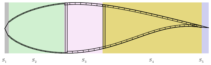
Figure 2 Cross-section of the NREL 5 MW wind turbine blade showing the segments used for thickness scaling.

A minimum manufacturable thickness constraint was formulated by considering the thickness of each layup in a segment and allowing the segment thicknesses to be scaled down until one layer reached the minimum manufacturable thickness. This constraint was applied to every cross-section, including between the control points. This added 25 design variables and 180 constraints to the optimization problem.

2.3.1 Power generation case

For the power generation case, we allow the optimizer to vary the tip speed ratio and the pitch of all 23 wind speeds. This accounts for 24 additional design variables. In total, this problem has 57 design variables. While a comprehensive blade optimization would include additional variable types, we limit the design space to maintain focus on demonstrating the derivative computation methods.

The objective function is the cost of energy. The cost of energy is estimated using the cost model in WISDEM (Fingersh et al., 2006; Harrison and Jenkins, 1994; Malcolm and Hansen, 2006; Maples et al., 2010):

$$\begin{array}{}\text{(3)}& \text{COE}={\displaystyle \frac{\text{FCR}\cdot \text{ICC}}{\mathrm{AEP}}}+{\displaystyle \frac{\text{OPEX}(\mathrm{1}-\mathrm{TR})}{\mathrm{AEP}}},\end{array}$$

where FCR is the fixed charge rate (assumed to be 0.1158), ICC is the initial capital cost, AEP is the annual energy production, OPEX is the annual operating expenses (assumed to be USD 144 000 per year), and TR is the tax rate (assumed to be 0.4). All of the assumed values in the cost model are based on values found in the implementation of the cost model in WISDEM (https://github.com/WISDEM/WISDEM, last access: 21 November 2025). The initial capital cost is calculated as

$$\begin{array}{}\text{(4)}& \text{ICC}=\text{BOS}+\text{TCC}+\text{WP},\end{array}$$

where BOS is the balance of station cost (assumed to be USD 2979 000), TCC is the turbine capital cost, and WP is the warranty premium (assumed to be 13 % of the turbine capital cost). The turbine capital cost is a summation of simple empirical models for the major components of the wind turbine, including the rotor, nacelle, and tower.

These models are dependent on various aspects of the design, such as the rotor diameter, the rated power, and the rated torque. The blade cost model is the most directly used in this optimization problem:

$$\begin{array}{}\text{(5)}& c_{\text{blade}}=\mathrm{14.6}{m}_{\text{blade}},\end{array}$$

where m_blade is the mass of the blade. The mass of each blade design is calculated by multiplying distributed weight (from the cross-section inertial data) of each beam element by the volume of the element (assuming that the density of each beam element is constant) and summing the result across the entire blade.

The AEP is calculated by integrating the power curve across a standard Weibull distribution with a mean wind speed of 6 m s⁻¹ and a shape parameter of 2.0. Since the power curve can be calculated via steady analysis, we perform this calculation just using CCBlade.jl (not including the entire aero-elastic solver). The power is constrained to be no greater than the rated power, and the thrust is constrained to be no greater than 600 kN at every wind speed. The thrust constraint is a surrogate for modeling the structural response of the tower. We also constrain the maximum rpm at each wind speed to 12. The power generation case contributes a total of 47 constraints to the optimization problem.

2.3.2 Parked extreme loading case

The second case, the parked extreme loading case, assumes a 50-year return-period wind speed of 70 m s⁻¹. Because the loading is treated as steady, the analysis shifts from a time-domain simulation to a steady aerodynamic analysis, with the dynamic stall model omitted. The resulting aerodynamic loads are applied directly to a steady-state beam model solution. The blade is assumed to be in its worst-case orientation (horizontal) with a pitch of 0°. The primary constraints for this case are buckling, ultimate strain, and tip deflection. The Bir buckling criterion is enforced at the top of each layer in the spar cap across all cross-sections, introducing 842 additional constraints. A conservative ultimate strain limit of 0.01 is applied to the top of every layer, in every segment, and across all cross-sections, resulting in 10 355 constraints. The ultimate strain limit incorporates a partial safety factor (γ_f) of 1.35 and a material safety factor (γ_m) of 1.1. The tip deflection is constrained to be less than the original design's overhang distance of 5.019 m with a safety factor of 1.15.

2.3.3 Dynamic turbulent inflow case

The third case is a dynamic turbulent inflow case. The turbulent inflow field is generated as specified in the pre-process step. We use the IEC Kaimal spectrum to generate a turbulent wind field with a 10 m s⁻¹ mean wind speed, a power law exponent of 0.2, and a surface roughness length of 0.03 m. The resulting wind field has an expected turbulence intensity of 0.16. Damage is extended from a simulation damage count to lifetime damage by simple scaling:

$$\begin{array}{}\text{(6)}& D=D_{\text{sim}}{\displaystyle \frac{t_{\text{lifetime}}}{t_{\text{simulation}}}}.\end{array}$$

The standard approach to calculating damage is by using a weighting of the lifetime damage from a range of different wind speeds. In this work, we calculate damage at only a single wind speed (the turbulent case at 10 m s⁻¹) to focus on demonstrating the capability to include fatigue damage in the optimization loop; full wind turbine design should consider the complete wind speed distribution. Furthermore, the damage analysis is only performed at key locations along the blade. While the strain analysis is relatively quick (93 ms), performing this analysis at every cross-section at every time step results in significant computational times. The damage was calculated at five locations along the blade: the root, the end of the cylinder section, and the three next-highest damage locations in the original design (25.79 %, 39.14 %, and 45.81 % of the blade length).

The IEC standard requires that damage be calculated based on 600 s of simulation in response to turbulent inflow. Typically, in OpenFAST, this is accomplished by running a 650 s simulation and removing the first 50 s of the simulation to allow the system to finish responding to the initial conditions (what we call the transient response). Including a 650 s simulation analysis in the optimization loop would result in significant computational times. To determine the length of simulation for the objective function, we swept the length of the simulation and experimented with several different cutoff times (see Fig. 3) when analyzing the initial design.

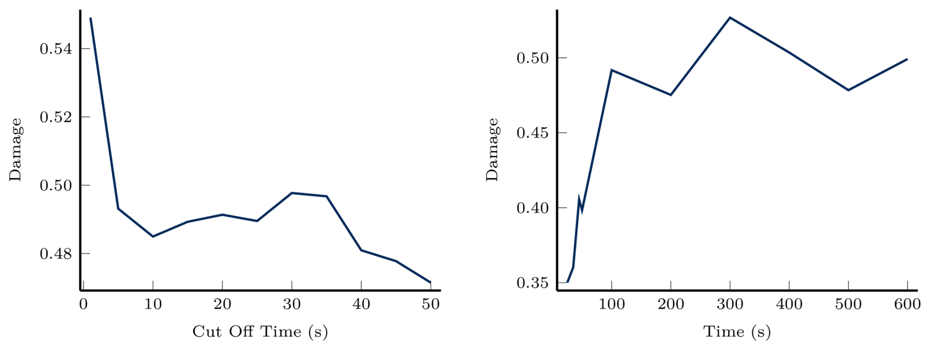
Figure 3 Left: varying the amount of time cut off from the beginning of the simulation. Right: varying the length of the simulation with the first 10 s removed.

The cutoff time was determined by running simulations of 600 s plus the portion removed at the beginning. Although the results did not demonstrate convergence at the standard 50 s cutoff, we selected a cutoff of 10 s for two reasons: (1) the relative percent difference in damage between all tested cutoff times and the standard 50 s cutoff was less than 3 %, and (2) including a cutoff reduces the influence of the transient response on the damage calculation. Extended cutoff times beyond 50 s showed no significant improvement in convergence, suggesting that the residual variation is inherent to the stochastic turbulent inflow rather than insufficient simulation duration. After fixing the cutoff at 10 s, we varied the total simulation length. A duration of 100 s was selected, as it was the shortest tested length yielding damage within 5 % of the 600 s result (specifically, within 1.48 %). The damage analysis introduces an additional 1811 constraints to the optimization problem. The damage metric exhibits high sensitivity to design changes, with values that can vary by multiple orders of magnitude. To improve optimizer performance, we apply a logarithmic transformation. Specifically, the damage is scaled by the safety factor (γ_fatigue=1.3), logarithmically transformed, and then constrained to be less than or equal to zero.

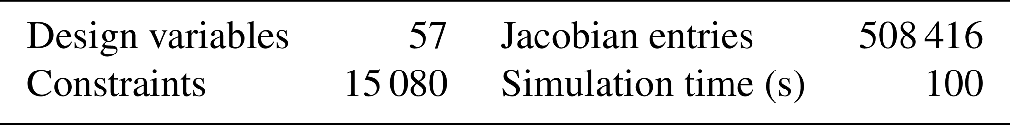
Finally, the tip deflection is constrained to be less than 90 % of the overhang distance at each time step throughout the same time period used for fatigue analysis. The simulation is run with a time step of 0.05 s, so the total number of time steps analyzed for fatigue and tip deflection is 1801. The size of the optimization problem is summarized in Table 1. The optimization problem is formulated as follows:

$$\begin{array}{}\text{(7)}& \begin{array}{rl}& \text{minimize: }\text{COE}\\ & \text{by varying: }{\mathit{c}}_i,{\mathit{\theta }}_i,{\mathit{s}}_n,{\mathit{\beta }}_j,\mathit{\lambda }\\ & \text{subject to: }\\ & \begin{array}{llll}{\mathit{P}}_j<P_{\text{max}}& {\mathit{T}}_j<T_{\text{max}}& \mathrm{\Omega }<{\mathrm{\Omega }}_{\text{max}}& {\mathit{\beta }}_j<{\mathit{\beta }}_{j+\mathrm{1}}\\ B_{\text{ult}}<\mathrm{1}& \frac{\mathit{\epsilon }}{{\mathit{\gamma }}_{\mathrm{f}}{\mathit{\gamma }}_{\mathrm{m}}{\mathit{\epsilon }}_{\text{ult}}}<\mathrm{1}& {\mathit{\delta }}_s<d_{\text{overhang}}& \\ {\mathit{\delta }}_k<\mathrm{0.9}{d}_{\text{overhang}}& \log (D/{\mathit{\gamma }}_{\text{fatigue}})<\mathrm{0}& \mathit{s}>s_{\text{min}},& \end{array}\end{array}\end{array}$$

where COE is the cost of energy, c is the chord length, θ is the aerodynamic twist angle, s values are the scaling factors of all of the layer thicknesses in a segment, β is the pitching angle, λ is the tip speed ratio, B_ult is a buckling constraint, ε_ult is an ultimate strain constraint, δ is a tip deflection constraint, d_overhang is the maximum allowable overhang distance, T_max is the maximum thrust force, Ω is the rpm (and corresponding constraint), D is the section damage constraint, and s_min is a minimum manufacturable thickness constraint. Note that the subscript i refers to values that vary across the blade, j refers to values that vary across wind speeds, and k refers to values that vary across time.

Table 1 Summary of optimization problem size. Note that the number of entries in the Jacobian is the number of non-zero entries.

3 Results and discussion

In this section, we demonstrate the capabilities of the approach. We begin with a verification case by comparing against OpenFAST. We then consider the performance of the differentiation approaches. We conclude with a discussion of the result of the optimization and how the differentiation approaches enable the inclusion of nonlinear fatigue analysis within the optimization loop.

3.1 Model verification

We verify WATT.jl by comparing its time-domain predictions with OpenFAST. The comparison consists of a 100 s simulation at 0.01 s time step with turbulent inflow averaging 10 ms⁻¹ and a rotor speed of 11.44 rpm. Other simulation details are provided in the companion repository. The verification focuses on three key blade responses: tip aerodynamic loading, tip deflection, and root flapwise bending moment. Figure 4 presents the first 50 s of these time histories, which captures the response variations while maintaining visual clarity.

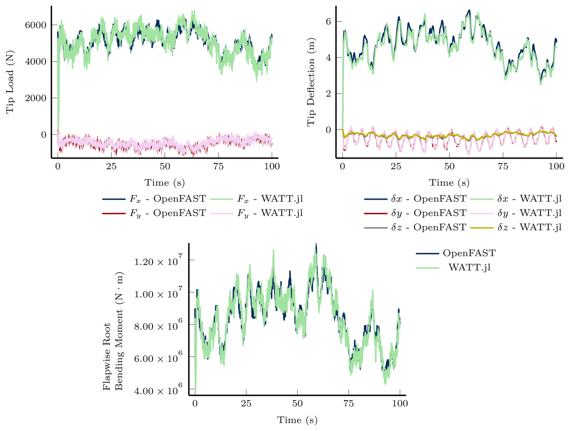
Figure 4 Comparison of the dynamic response to turbulent inflow of the NREL 5 MW wind turbine blade using OpenFAST and WATT.jl.

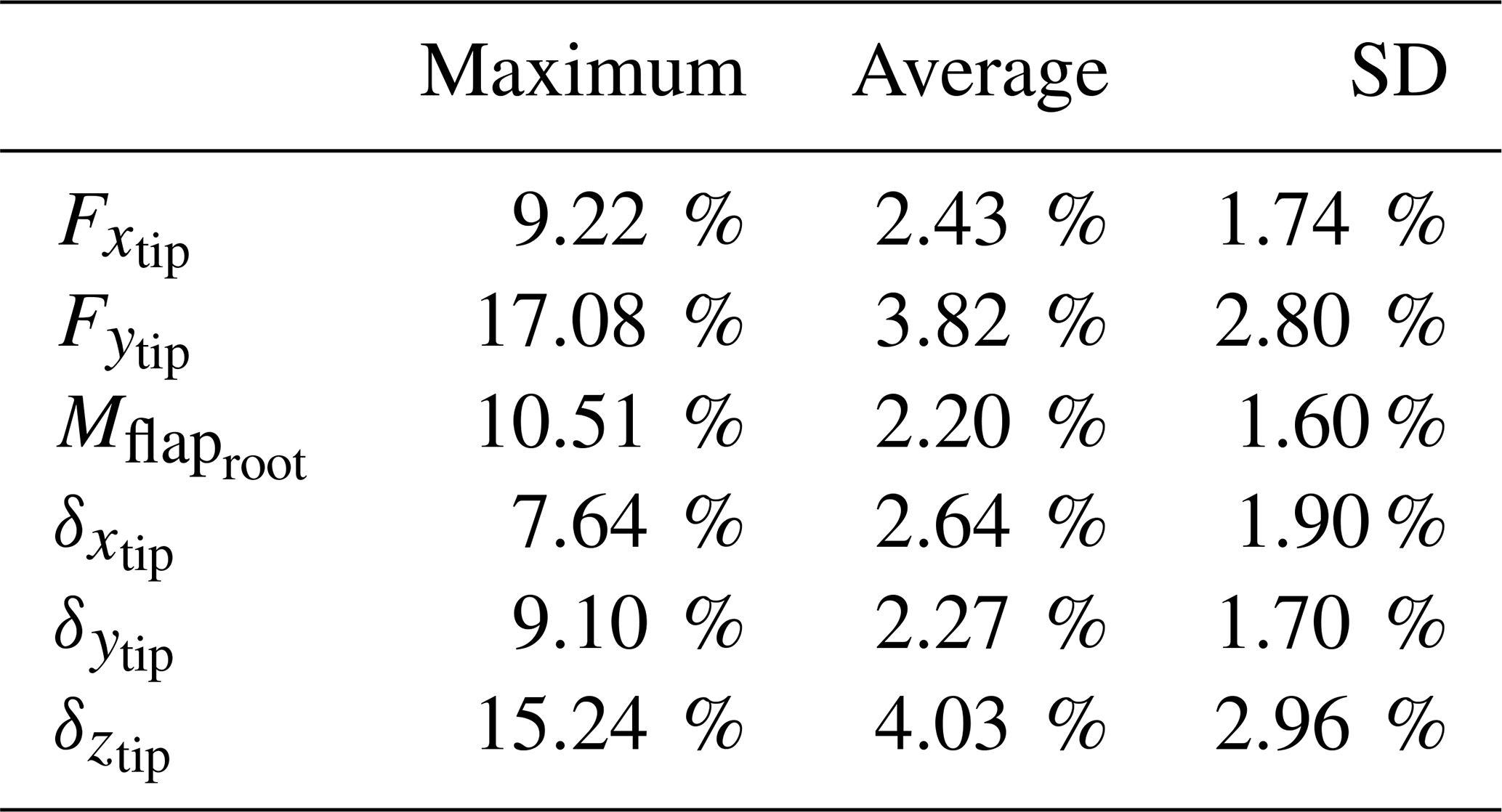
In general, this figure demonstrates fairly good agreement between the two models. To quantify their performance, we provide an error comparison. Because the lead–lagwise tip deflections frequently cross zero, we compare all blade responses using a maximum normalized relative error. We define the normalized error between two vector quantities as

$$\begin{array}{}\text{(8)}& {\mathit{E}}_i\left(\mathit{a},\mathit{b}\right)=\mathrm{100}{\displaystyle \frac{{\mathit{a}}_i-{\mathit{b}}_i}{\mathrm{sign}\left({\mathit{b}}_i\right)\left|\right|\mathit{b}|{|}_{\mathrm{\infty }}}},\end{array}$$

where E, a, and b are all vector quantities. The index i refers to the vector element being evaluated, and the infinity norm is applied to all elements of b. We use the normalized error for all comparisons for consistency. To provide interpretable results across time, we provide basic statistics on the normalized error, including the maximum, average, and standard deviation. The statistics of the aero-structural response are from 10 to 100 s to omit the transient response. Based on the results summarized in Table 2, we conclude that the two codes are in sufficient agreement for design optimization.

Table 2 Normalized error statistics between OpenFAST and WATT.jl.

Before examining derivative performance, we compare the computational costs of OpenFAST and WATT.jl. In the analysis shown in Table 2, the codes perform similarly: OpenFAST averages 67.3 s, while WATT.jl averages 65.2 s. The performance changes at larger time steps. When increased to 0.05 s, OpenFAST fails to converge, whereas WATT.jl completes the analysis in 13.1 s. WATT.jl's robust structural solver enables this larger time step without sacrificing accuracy – results remain within one percent of those obtained with the finer discretization. Simulations were conducted on a MacBook equipped with a 2.6 GHz six-core Intel i7 CPU and 32 GB of RAM.

3.2 Derivative performance

In this section, we examine how well the differentiation approaches from Sect. 2.2 perform when used in the optimization problem outlined in Sect. 2.3. We demonstrate the efficiency by first showing the derivative computation times of the different methods and then by showing how the methods scale with the number of design variables. We compare six different combinations of differentiation methods:

1. a centered finite difference,

2. forward-mode AD,

3. forward-mode AD with implicit differentiation around solvers,

4. reverse-mode AD with implicit differentiation and constraint aggregation,

5. parallelized forward-mode AD with implicit differentiation, and

6. parallelized sparse forward-mode AD with implicit differentiation.

3.2.1 Derivative computation times

Table 3 shows the wall time and number of allocations of the six different differentiation techniques. We discuss four different features of Table 3.

Table 3 Wall times to compute the Jacobian with a 100 s simulation for fatigue analysis.

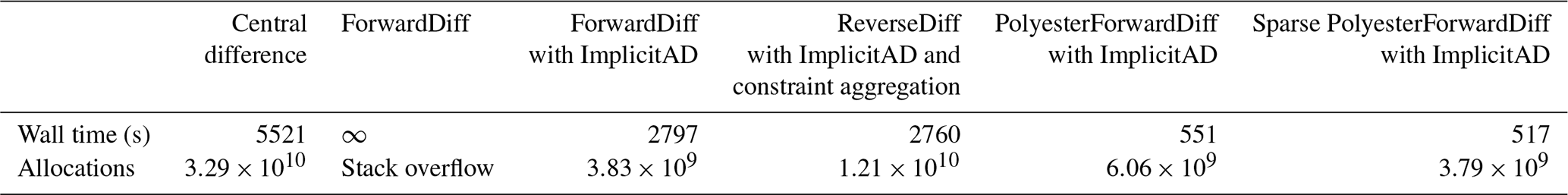
First, we see that if we naively apply forward-mode AD to the optimization problem, the stack memory requirements quickly become untenable, specifically when propagating derivatives through the nonlinear solver inside of the time-domain portion of the structural model. These memory issues are not inherent to forward-mode AD with iterative solvers in general but arise from our specific implementation. The structural model we use, GXBeam.jl, is optimized to utilize stack memory for efficient structural analysis by storing variables on the stack rather than on the heap. ForwardDiff.jl tracks derivatives by augmenting each scalar variable with additional derivative information, effectively replacing each number with a small data structure containing both the value and its derivatives. When GXBeam.jl's many stack-allocated variables are augmented with this derivative information, the stack memory capacity is quickly exceeded. Applying implicit differentiation around the iterative solves circumvents this issue by computing derivatives without propagating them through the solver iterations, making AD feasible. GXBeam.jl was designed with implicit differentiation methods in mind so that it can benefit from both the speed of stack memory and the accuracy of AD.

Second, we see a variation in memory usage across the different methods. The number of allocations is not a reflection of how much information is held in memory at once but how much the memory is being used. The reverse-mode method offers a modest reduction in wall time compared to the forward-mode method, at the cost of increased memory usage. However, the increased memory requirements are lower than what a centered finite difference demands. The parallelization of the derivatives provides the largest speedup but requires more allocations than plain forward-mode AD. This is because extra memory must be allocated to avoid data race conditions.

Third, there is opportunity for further speedup of the finite differencing by using more compute resources, specifically the number of threads used in the derivative computation. If memory is not a limiting factor, then theoretically the number of threads could be increased to the number of design variables times 2 (for centered finite differencing). This would reduce the wall time to be about the time it takes for a single function evaluation (about 48.43 s with 114 cores for this problem). Even though modern HPC resources could provide enough threads to make this cost tractable for small problems, they cannot improve the limited accuracy of finite differencing. Higher-order finite-difference schemes can improve derivative accuracy, but such methods are often impractical for large problems. Ultimately, the trade-off between computational resources and real-time performance is an engineering decision, where derivative accuracy remains a critical factor. Additionally, while higher-order finite-differencing schemes can improve the accuracy of the derivatives, they will always be limited by the truncation and round-off errors associated with finite differencing.

Fourth, the sparse method is the fastest method tested for the original optimization problem, over an order of magnitude faster than a centered finite difference. The sparse method is faster than the parallelized method because the sparsity means the method is solving a smaller problem. Because of the relatively low cost of evaluating the power generation case, we separate gradient evaluation from the Jacobian evaluation. Thus, we are able to color the Jacobian and compress the number of columns from 57 to 35 (a reduction of 22 columns or 38 %). The gradient is evaluated using reverse-mode differentiation, which takes about 0.1 s. The Jacobian is evaluated using parallelized forward-mode AD, which takes the rest of the time for the sparse differentiation method.

3.2.2 Derivative scaling

To demonstrate how the different methods scale with the number of design variables, we performed two types of sweeps: (1) varying the number of control points used in the chord and twist parameterizations and (2) varying the number of wind speeds analyzed in the power generation case. The first sweep increases the number of dense columns in the Jacobian, while the second sweep increases the number of columns that can be colored (see Fig. 5). Each method was evaluated 10 times, and the wall times were averaged. We compare methods by examining wall time increase per additional design variable. All methods exhibit approximately linear scaling (O(n)). Note that forward-mode AD without implicit differentiation is omitted due to prohibitive stack memory requirements.

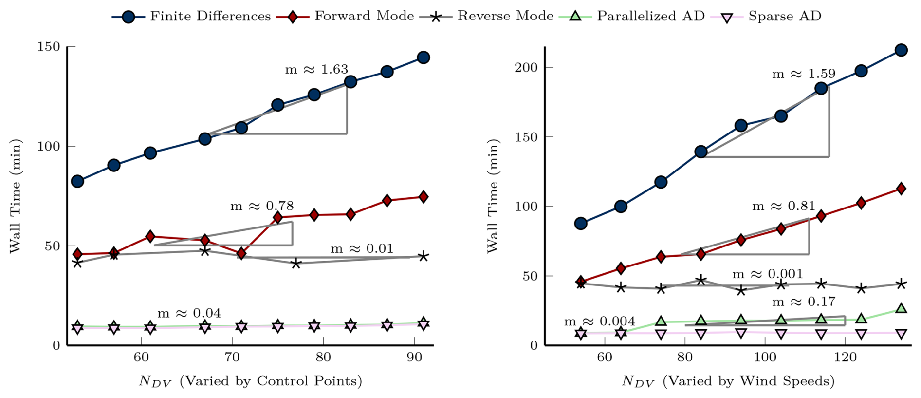
Figure 5 Scaling of derivative computation wall times with number of design variables. Left: varying the number of chord and twist control points. Right: varying the number of wind speeds analyzed in the power generation case.

The finite-difference method had the worst scaling in both sweeps. The small difference in the slopes for the two sweeps, 1.63 and 1.59 for the control point sweep and the wind speed sweeps respectively, is likely due to the relatively small sample size used in timing. Parallelizing the finite difference would dramatically increase the scaling of the method at the expense of an obvious increase in computational resources.

Forward-mode AD with implicit differentiation demonstrates superior scaling compared to finite differences, with an average slope of 0.795. This improvement stems from the reduced number of mathematical operations required. Centered finite differences evaluate each operation 1+2N times: once for the primal and twice (forward/backward perturbation) for every N design variables. Forward-mode AD evaluates each operation 1+N times: once for the primal and once per derivative direction. In ForwardDiff.jl, the primal is recomputed for each chunk, so each operation is repeated $\mathrm{ceil}\left(N/\text{chunk size}\right)+N$ times. With the application of implicit differentiation to the iterative solvers, the iterated operations are only evaluated for the primal solve and not for the derivative computation (although the residual is evaluated once for each derivative). Additionally, since the entire code is evaluated fewer times, there are improved memory savings from re-allocating vectors fewer times.

The reverse-mode derivative with implicit differentiation and constraint aggregation method has the best scaling in both sweep cases, 0.01 and 0.001. This is expected because of the fact that reverse-mode differentiation scales with the number of outputs, not the number of inputs. Since the constraints are aggregated into a single constraint, they can be calculated with a single pass. The differences in scaling between the two cases are likely due to the sample size and locations (i.e., if there were more samples, we would likely see a more consistent slope for the two methods). We do expect to see a slope (and some slight differences in the slope) because there is increased computational costs and memory overhead associated with evaluating a larger primal function. We note that in an optimization setting, instead of aggregating all constraints into a single constraint, you may seek more accuracy in your constraints and so you may aggregate constraints by type. In this case, you can decrease wall time by parallelizing constraint gradient computation.

The parallelized forward mode with implicit differentiation method has the next best scaling. The parallelized forward-mode AD method scales better than the forward-mode AD method because, as the number of columns increased, we increased the number of CPU cores available. To demonstrate the effect of not using an optimal number of cores, we used a constant number of cores in the second sweep. In the first sweep, the slope was 0.03, but the slope for the second sweep was 0.17. You can see two sections where the wall time increases (when it jumps from 64 to 74 design variables and when it jumps from 123 to 134 design variables). Since the chunk size is eight and the sweep uses eight CPU cores, we expect there to be jumps in the wall time when the number of design variables surpasses multiples of 64 (64, 128, 192, etc.). What is happening here is that every 64 design variables, the processors have to run another batch of derivatives in order to calculate all of the columns of the Jacobian. You can avoid these jumps by using more processors or increasing the chunk size. Recall that increasing the chunk size will increase memory requirements and may result in slower derivative computation times. Experimentation is required to determine the optimal chunk size to processor ratio. Outside of the jumps, the scaling of the second sweep is 0.04 (calculated by looking at just the wall times in between the two jumps). The slope of 0.17 is still better than the plain forward-mode method with implicit differentiation because there are more CPU cores working on the problem.

Finally, we consider the sparse parallelized forward mode with implicit differentiation method for calculating derivatives. Note that the slope goes from 0.04 for the first sweep to 0.004 in the second sweep. The slope improves greatly from the first sweep to the second sweep because adding wind speeds adds structurally orthogonal columns to the Jacobian. For this method, this means the only added cost is the added cost of calculating the primal values for the new analyses (in a similar fashion to the reverse-mode method). We note that for the second sweep, we also held the number of CPU cores constant, but because the number of columns of the Jacobian did not effectively change, we do not see any jumps in the wall time.

The techniques presented here can benefit gradient-based optimization across various applications, though implementation considerations differ depending on your starting point. For those developing new analysis tools, incorporating AD compatibility from the outset lays the groundwork for efficient gradient-based optimization. This early consideration should be balanced alongside other design decisions, such as ensuring numerical stability and convergence robustness. For existing codebases where restructuring for AD compatibility may be impractical, techniques like parallelization and exploiting sparsity offer more accessible performance improvements that do not require fundamental code changes. Tests are recommended as scaling is problem dependent.

3.3 Optimization results

To assess the practical effectiveness of the parallelized sparse forward mode with implicit differentiation method, we present two optimization studies. Our first study, a baseline optimization starting from the initial design, shows that the optimization produces realistic results and improves upon finite-difference approaches. The second study is a set of multiple optimizations from random starting points that verify that the derivatives remain stable and consistent across different regions of the design space. We primarily focus on the parallelized sparse forward mode with implicit differentiation (which we occasionally refer to as the sparse method for brevity) because it was the fastest for the problem sizes we checked.

3.3.1 Baseline optimization

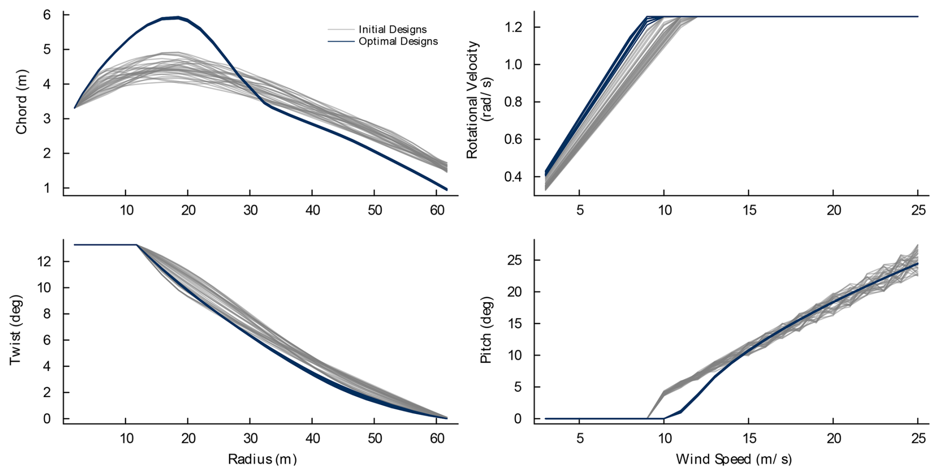
First, we consider the optimal design and then discuss the performance of the baseline optimization in comparison to a finite-difference approach. The optimization results are summarized in Table 4, and the optimal design is shown in Fig. 6.

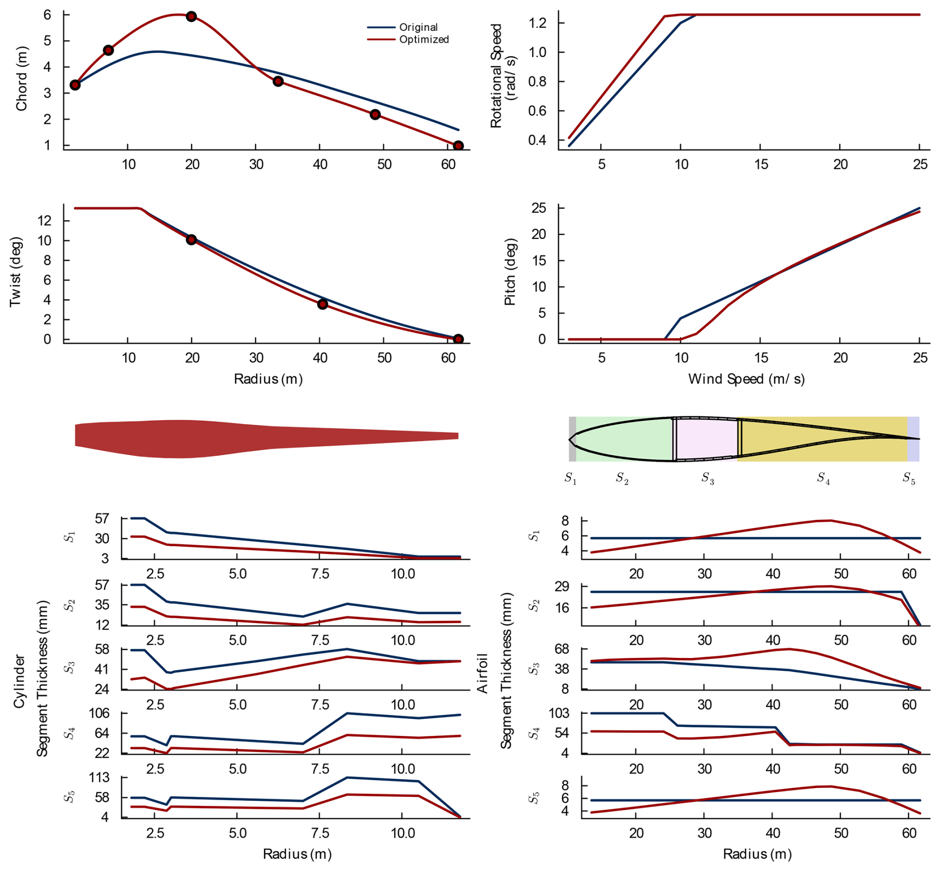
Figure 6 Reference optimization optimal design. Markers indicate the locations of the control points.

Table 4 Summary of optimization results. The number of active constraints is given at the initial (Con_i) and optimal (Con_opt) designs.

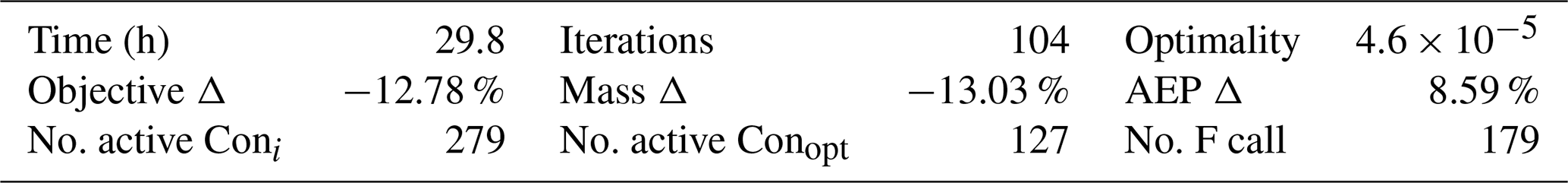
We performed the baseline optimization in 29.8 h using eight 2.45 GHz AMD EPYC 7763 CPU cores with 7 GB of RAM from the Fulton HPC resources at Brigham Young University. The optimization converged in 104 iterations to an optimality of $\mathrm{4.6}\times {\mathrm{10}}^{-\mathrm{5}}$, representing the infinity norm of the Lagrangian gradient. The objective function (COE) decreased by 12.78 % through a 13.03 % mass reduction and 8.59 % increase in annual energy production (AEP). The initial design had 279 active constraints, while the optimal design had 127 active constraints. The optimizer required 179 function calls, including line search evaluations.

When considering the optimal design, we highlight four design trends. We note that since the focus of our work is the optimization efficiency and robustness, we only provide a brief discussion of these trends. First, in Table 4, we see that the change in blade mass outweighs the change in annual energy production. Consistent with other studies (Yao et al., 2022), the material in the blade (and thus the mass) is the primary driver of decreasing the cost of energy. Second, in Fig. 6, we see a trade-off between the chord and the twist. We see that the chord is increased at the inboard region of the blade, whereas it is decreased near the outboard region. In the outboard regions the twist is also decreased. We see a similar trend in analytic aerodynamic-only optimal solutions (see Burton et al., 2011, for an example of the analytic BEMT optimal solution). However, as seen in Fig. 7, the solution does not reach the aerodynamic-only solution because the objective function prioritizes cost reduction rather than pure aerodynamic performance. Third, we see a trade-off between the chord and layer thicknesses. We see that in the inboard region, especially in the cylinder region, the layer thicknesses shrink in response to the increased chord. The larger chord is better able to resist the loads applied there, so the thicknesses can be reduced there to decrease the mass. Fourth, the optimized design has a delayed initiation of the blade pitch controller as compared to the initial design. Delaying pitch increases the loading, which in turn increases the torque, resulting in higher power generation. It is important to recognize that since the optimization considers design variables that affect both the design and the control of the wind turbine, it must also analyze the effects they have on each other so that they are co-designed.

Of the 127 active constraints at the optimal design, 28 were minimum-manufacturable-thickness constraints, 1 was the static deflection constraint, 7 were pitch monotonicity constraints, 15 were max power constraints, 73 were buckling constraints, 1 was the max thrust constraint, and 3 were fatigue constraints. The buckling constraints were active in three sections near the hub ranging from 1.9 to 2.1 m. The active fatigue constraints were all located in the trailing-edge segment of the cross-section at the end of the cylinder section. This is typical (see Bortolotti et al., 2016), as the trailing edge typically experiences the largest-amplitude strain oscillation.

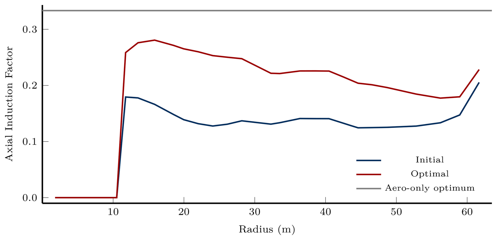
Figure 7 Axial induction factor distribution along the blade from steady aerodynamic-only analysis at rated wind speed (11.4 m s⁻¹).

Comparing our approach to finite difference highlights significant practical advantages. The AD-based optimization converged to an optimality of $\mathrm{4.6}\times {\mathrm{10}}^{-\mathrm{5}}$ in 29.8 h. From Sect. 3.2, we see that finite-difference gradients are approximately 10× slower than the parallelized sparse approach. Assuming that the optimizer would follow the same trajectory as when using the sparse approach, this implies that similar convergence would require roughly 298 h or just over 12 d. To compare against this projection, a centered finite-difference optimization was attempted directly. It failed within the first few iterations. The inherent error in finite-differenced derivatives exceeded the optimizer's default tolerances for gradient noise, causing premature termination before the optimization could progress. While careful hyperparameter tuning and scaling might enable some degree of convergence, reaching the same optimality achieved with accurate AD derivatives would be unlikely. The baseline optimization establishes two key findings: the derivative methods yield physically realistic designs in an optimization, and they significantly outperform finite difference. Single-point convergence alone, however, cannot establish derivative stability throughout the design space.

3.3.2 Multi-start optimizations

The second study evaluates derivative stability across the design space through multi-start optimization. Multi-start optimization is a well-established technique for robustly locating global optima (Chew et al., 2016; Rodrigues et al., 2024; Santa, 2024), and convergence behavior under this framework provides insight into gradient reliability. Consistent convergence from diverse starting points within the same basin of attraction indicates reliable derivatives, whereas chaotic or inaccurate gradients would prevent the optimizer from repeatedly reaching the same solution. We generated 50 starting designs by randomly perturbing all initial design variables within ±10 % of their baseline values. Design variable perturbations have small magnitudes such that starting designs are likely to occupy the same basin of attraction as the original design. We selected the sample size as it approximates the dimensionality of the optimization problem. Of the 50 runs, 34 optimizations converged smoothly and 16 failed due to structural analysis instabilities. The following analysis addresses converged cases first, followed by the non-converged cases.

The converged optimizations shown in Fig. 8 demonstrate remarkable consistency. The optimal designs cluster tightly together, with the optimal chord exhibiting an average standard deviation of just 1.08 cm. Such tight convergence indicates that the derivatives are both accurate and consistent across a sizable portion of the design space that the optimizer explored. While a stricter optimality tolerance could reduce this variability, doing so could substantially increase iteration counts and might necessitate stopping and rescaling design variables. If the optimizations were conducted with noisy or inaccurate gradients, we would expect to see a wider spread in the final designs.

Figure 8 Optimizations from different starting points converging to one solution.

A total of 16 randomly generated starting points failed to converge due to numerical instabilities in the unsteady aero-structural analysis, particularly within the structural solver. These failures typically stem from highly elastic blade designs that create positive feedback loops with the aerodynamic model. A finer temporal mesh generally resolves such instabilities. These failure modes are characteristic of the underlying physics and solver performance rather than deficiencies in the derivative computation. The gradients accurately reflect the challenging landscape near infeasible designs. The 34 converged cases validate derivative consistency in the feasible and near-optimal regions.

4 Conclusions

Gradient-based optimization is an effective approach to creating wind turbine blade designs that not only meet performance requirements but also minimize cost. The cost of calculating derivatives has historically made it infeasible to conduct nonlinear time-domain simulations to include fatigue analysis within the optimization loop. We use efficient derivative computation methods to allow for the inclusion of fatigue analysis within the optimization loop.

We evaluate six differentiation approaches: finite differences, forward-mode AD, forward-mode AD with implicit differentiation, reverse-mode AD with implicit differentiation, parallelized forward-mode AD with implicit differentiation, and sparse parallelized forward-mode AD with implicit differentiation. Using a proof-of-concept optimization problem, we compare computational costs and examine how each approach scales with problem size. The sparse parallelized forward-mode approach proves to be over an order of magnitude faster than traditional finite differences. Since this approach computes derivatives using algorithmic differentiation, it avoids the truncation and cancellation errors associated with finite differences, generally yielding more accurate gradients. Sparsity and parallelization reduce the computational cost further while preserving this accuracy advantage. The approach also exhibits favorable scaling characteristics as problem size increases.

To allow for AD compatibility, we present a new aeroelastic solver: WATT.jl. Similar to OpenFAST, the solver incorporates blade element momentum theory, the Beddoes–Leishman dynamic stall model, and a geometrically exact beam theory structural solver in a fully nonlinear two-way-coupled partitioned model. The analysis method is compared to OpenFAST and is within an average of 2 %–4 % of the time-domain loads and deflections. Additionally, classical laminate theory, the rainflow counting algorithm, and linear damage accumulation methods are integrated into the analysis framework.

The derivatives are used in a representative optimization problem to demonstrate feasibility. The optimization converges to an optimality of $\mathrm{4.6}\times {\mathrm{10}}^{-\mathrm{5}}$ in 29.8 h using only eight CPU cores and 7 GB of RAM. The cost of energy objective is reduced by 12.78 % by reducing the blade mass by 13.03 % and increasing the AEP by 8.59 %. Future work should include the exploration of additional design variables and constraints to better capture the complexities of the full wind turbine design problem. Because of the few resources required, it should be straightforward to scale up the problem to include more design load cases and a more complex design space.