Temperature profiling at the American WAKE ExperimeNt (AWAKEN): methodology and uncertainty quantification

We quantify the accuracy of the temperature profiling from ground-based spectral infrared radiance observations at the American WAKE ExperimeNt (AWAKEN). Results from pre-campaign tests and comparisons with in-situ ground-based and airborne sensors at AWAKEN indicate that temperature profiles agree satisfactorily with traditional instruments for wind energy applications. The bias is within a fraction of a degree and appears to be related to atmospheric stability. Root-mean-square differences from the reference instruments are always smaller than a degree and are often well described by the online uncertainty estimation product. Height-to-height and site-to-site temperature differences are in excellent agreement with in-situ observations, which justifies the use of temperature profilers to characterize static stability and spatial gradients of temperature.

1 Introduction

An accurate characterization of the atmospheric state is essential in understanding the mechanisms that govern the conversion of the flow of kinetic energy carried by the wind into mechanical and, ultimately, electrical power delivered to the grid by wind power plants. In fact, although wind energy represents a widely available resource and an established technology across the United States, globally, it introduces new challenges to the global power system due to its intermittency and uncontrollability. These are becoming more pressing concerns as the worldwide electricity demand grows by 4 % annually, driven largely by electrification, air-conditioning needs, and data centers (International Energy Agency, 2025).

The volatility of wind power is inherently connected to the complex dynamics of the atmospheric boundary layer (ABL) in which wind turbines operate. The ABL state is extremely difficult to predict, and current wind resource models still have significant biases (Lee and Fields, 2021; Bodini et al., 2024). A recent blind comparison of several turbine models attributed a large portion of the uncertainty to incomplete information regarding the inflow conditions, especially when the ABL is stably stratified (Doubrawa et al., 2020). Complexity of the wind field is further enhanced as the thermally stratified ABL interacts with even modest terrain features (Mahrt et al., 2021; Radünz et al., 2025) or the turbines themselves (Krishnamurthy et al., 2025; Abraham et al., 2025).

Atmospheric stability not only plays a role in shaping the undisturbed wind profiles experienced by the turbines but also governs the propagation of wind turbine wakes, with large implications for the overall efficiency and lifetime of the wind plant. This influence of thermal stratification on wake morphology has largely been proven in numerical (e.g., Abkar and Porté-Agel, 2015), lab-scale (e.g., Chamorro and Porté-Agel, 2010), and field-scale studies (e.g., Zhan et al., 2019).

The importance of atmospheric stability within the physics of wind energy has prompted many experts to advocate for a more comprehensive experimental characterization of the key quantities that govern the physics of the atmosphere, with particular emphasis on those that carry information regarding the thermal state of the ABL, primarily temperature profiles (Veers et al., 2019; Shaw et al., 2022).

Better knowledge of the temperature profiles around operating wind power plants could also help to elucidate a long-standing question about the effects of wind turbine wakes on local climate. Early coarse simulations of global weather patterns with extremely large wind penetrations showed potential climate impacts (Keith et al., 2004; Wang and Prinn, 2010; Li et al., 2018; Miller and Keith, 2018). However, experimental work using satellite-derived surface temperatures (Zhou et al., 2012, 2013; Xia et al., 2016; Liu et al., 2023; Walsh-Thomas et al., 2012) or observations near the ground (Baidya Roy and Traiteur, 2010; Rajewski et al., 2013; Smith et al., 2013; Moravec et al., 2018; Wu and Archer, 2021) highlighted temperature differences of generally less than 1 °C that appear to be induced by turbines. The general consensus is that turbines cause surface warming during nighttime stably stratified conditions, while daytime data draw a more uncertain picture. More recent meso- and micro-scale computational fluid dynamics studies proposed sound physical explanations for the thermal effects of wind turbines (Xia et al., 2019; Wu et al., 2023), especially thanks to the access to simulated vertical temperature profiles. However, observations of the thermal effects of wind turbines across multiple heights to support such hypotheses are still scarce.

Finally, a more practical but nevertheless important use of temperature information for wind energy is the estimation of air density profiles across the turbine rotor span, which is essential in assessing the energy yield and conducting power performance tests on wind turbines (International Electrotechnical Commission, 2022).

Based on the former discussion, temperature profiling has been one of the foci of the American WAKE ExperimeNt (AWAKEN, Moriarty et al., 2024), the largest experimental field campaign for wind energy conducted in the United States to date. At the AWAKEN site, temperature profiles were routinely measured through an innovative remote-sensing tool, which combined the observations from infrared spectrometers and historical radiosonde data to estimate vertical profiles of temperature throughout the ABL and beyond. Specifically, spectrometers called Atmospheric Sounder Spectrometer by Infrared Spectral Technology (ASSIST, Michaud-Belleau et al., 2025) by LRTech were deployed at several locations throughout the AWAKEN domain and recorded the downwelling spectral infrared radiance at the ground level. The physical retrieval algorithm Tropospheric Remotely Observed Profiling via optimal estimation (TROPoe, Turner and Blumberg, 2019; Turner and Löhnert, 2014; Adler et al., 2024) was then used to estimate temperature profiles that matched the observed radiance. The combined ASSIST–TROPoe system represents a thermodynamic profiler.

The AWAKEN project hosted the first large-scale deployment of thermodynamic profilers for wind energy research and included extensive validation. The TROPoe methodology is briefly described in Sect. 2, while the following sections discuss the details of the validation process. In the pre-campaign phase, two identical thermodynamic profilers were installed side by side to assess the magnitude of instrumental noise and calibration error (Sect. 3.2). The temperature estimated by the thermodynamic profilers was also compared to observations from a nearby meteorological (met) mast to quantify the overall error across different heights, mainly in the surface layer (Sect. 3.3). Later on, during AWAKEN, temperature profiles from a thermodynamic profiler were validated compared to radiosonde measurements, providing a comprehensive error quantification across the entire ABL (Sect. 4.2). Finally, differences in temperature between sites were compared to the same quantities observed by independent and co-located surface met stations to assess the ability of temperature profiling to characterize the spatial heterogeneity of the temperature field (Sect. 4.3). The key takeaways are provided at the end of each section, and overall conclusions are drawn in Sect. 5.

2 Methods

The temperature profiling method used at AWAKEN relies on the information regarding temperature and humidity profiles contained in the downwelling infrared spectral radiance observed on the ground by the ASSIST. This information, as shown in Fig. 1, is then combined with ancillary measurements (e.g., the cloud base height or CBH from a ceilometer) and used by TROPoe to estimate the thermodynamic state that agrees with the observed infrared radiance and has the highest likelihood based on the current observations and constrained by past climatology. The retrieved thermodynamic state includes the vertical temperature profile, as well as humidity and cloud properties, although we will focus on the first quantity in the present study. This section will review the fundamentals of temperature profiling at AWAKEN. For a more detailed discussion, refer to Letizia et al. (2025) and the references listed therein.

2.1 Instrumentation

The ASSIST is a hyperspectral infrared spectrometer that resolves the downwelling radiation in the wavenumber range 525–3300 cm⁻¹ with a spectral resolution of about 0.5 cm⁻¹. It shares many similarities with the older Atmospheric Emitted Radiance Interferometer (AERI, Knuteson et al., 2004a). In fact, the core instrument is a Fourier transform interferometer of the Michelson type. The online radiometric calibration is carried out by rotating a scene mirror that alternates views of two blackbodies and the sky. One blackbody is thermally regulated, and the other is allowed to drift according to the ambient conditions, and both act as known sources of emission in the linear calibration process. The ASSIST is able to generate an independent spectral radiance estimation every ∼14 s during sky views. High spectral accuracy is obtained thanks to a stable laser source that triggers the sampling of the raw interferogram at precise intervals along the mirror path. The interested reader is referred to Michaud-Belleau et al. (2025); Letizia et al. (2025) for more details.

2.2 Physics of radiation in the atmosphere

The spectral radiance observed at the ground, B, and the current thermodynamic state of the atmosphere are connected through the physics of infrared radiation. In fact, each layer in the column of air directly overhead the instrument emits infrared radiation based on the local temperature and proportionally to the local absorption coefficient, which varies spectrally due to the chemical–physical properties of various trace gases like water vapor and carbon dioxide. The volume of air between each emitting layer and the observer at the ground, in turn, absorbs and scatters the downwelling emission, also based on the local absorption coefficient. The latter is the physical parameter that quantifies the opaqueness of a medium to incident radiation and is highly dependent on the wavenumber, $\stackrel{\mathrm{̃}}{\mathit{\nu }}$, of the radiation itself (Siegel, 1971). In general, more opaque wavenumber regions will only allow emissions close to the observer to reach the ground-based spectrometer. Conversely, transparent wavenumber regions will let radiation emitted from higher altitudes be detected by the instrument. These properties are exploited to infer the vertical distribution of temperature profiles based on the spectral behavior of the radiance passively measured at the ground.

TROPoe utilizes a spectrally resolved and extensively validated radiative transfer model (Turner et al., 2004; Clough et al., 2005; Mlawer and Turner, 2016) to simulate the spectral radiance that is associated with a given thermodynamic profile (mainly temperature and water vapor content). The model includes a detailed description of the physics of radiation and the molecular mechanisms that govern the absorption and/or emission at different wavenumbers. The main task of the thermodynamic retrieval algorithm is then to solve the inverse radiative transfer problem based on the observations, which is an ill-posed mathematical operation. The solution method for this challenging problem is described next.

2.3 Fundamentals of TROPoe

Calculating the spectral radiance for a given temperature profile represents a complex but relatively established task; however, the inverse problem is significantly more challenging. Unlike other remote sensing instruments like lidars and radars, the ASSIST is completely passive in the sense that it does not emit any electromagnetic pulse that could be used to perform ranging, for instance, based on the time of flight. Instead, it observes only the radiation at the ground, whereas the estimation of the associated temperature profiles is done in a purely mathematical way by inverting the radiative transfer problem, which is an integral equation. This can be seen as the impossible task of guessing the shape of a solid object by just looking at its shadow.

TROPoe uses optimal estimation techniques (Rodgers, 2000; Turner and Löhnert, 2014) that leverage the statistical information on the temperature profiles collected by previous radiosonde launches to constrain the problem and converge to a unique solution. Specifically, the mean and level-to-level covariance of temperature, T, and water vapor mixing ratio, r, at different heights, z, are compiled into the so-called prior. The use of optimal estimation not only facilitates the convergence of TROPoe to a realistic solution but also provides the posterior covariance as an output, which quantifies the uncertainty of the retrieval. The embedded uncertainty quantification represents an advantage of TROPoe compared to regression or machine-learning-based methods for temperature profiling. The full details of TROPoe are given in Turner and Löhnert (2014); Turner and Blumberg (2019).

The process just described is depicted in Fig. 1, and it is generally more complex and computationally expensive than other techniques used to observe atmospheric quantities using in situ or remote sensing devices. However, physical–iterative retrieval frameworks like TROPoe have several advantages that more statistically based retrieval methods do not (Maahn et al., 2020; Letizia et al., 2025), such as the embedded uncertainty estimation, a broader generality, and easier troubleshooting. Understanding the limitations of temperature profiling is, indeed, crucial for an informed use of the data products. Therefore, the following section discusses the possible sources of uncertainty associated with our temperature profiling.

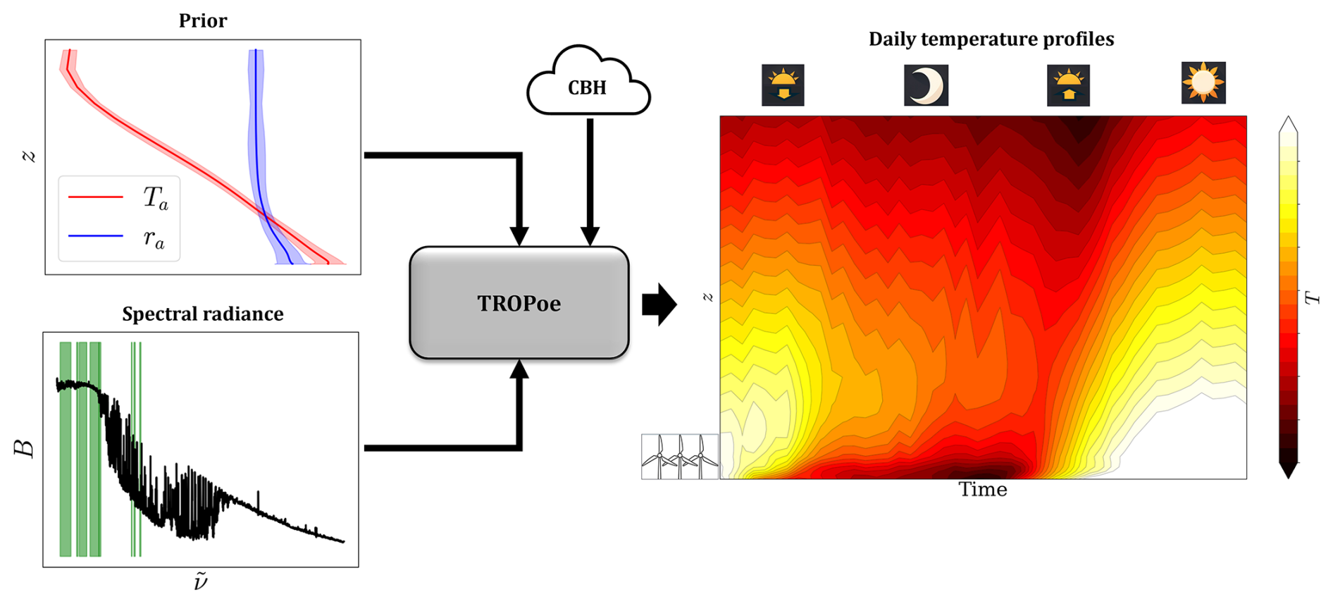
Figure 1 Workflow of temperature profiling. The green bands in the spectral radiance are those used for AWAKEN.

2.4 Sources of uncertainty

When discussing the accuracy in temperature profiles, it is important to distinguish between known and unknown uncertainties. The former are included in the posterior covariance generated by TROPoe, and the latter are not. The known error can be expressed as follows (Rodgers, 2000):

$$\begin{array}{}\text{(1)}& \widehat{x}-x=\stackrel{\text{smoothing}}{\overbrace{(\mathbf{A}-\mathbf{I})(x-x_a)}}+\stackrel{\text{noise}}{\overbrace{\mathbf{G}\mathit{ϵ}}},\end{array}$$

where

• $\widehat{x}$ is the estimated state (i.e., estimated temperature profiles);

• x is the true state (i.e., real temperature profiles);

• I is the identity matrix;

• A is the so-called averaging kernel or A-kernel, an important output of TROPoe;

• G is the so-called gain matrix, an intermediate product of TROPoe;

• ϵ is the noise on the observations (i.e., on the spectral radiance).

The known error is therefore the sum of the effect of smoothing and noise. The smoothing is a typical source of uncertainty in optimal-estimation-based atmospheric sounding. The retrieved profiles are, in fact, a smoothed version of reality with a vertical resolution that is roughly equal to the height above the ground level. This makes temperature profiling more accurate close to the ground (where, for instance, wind turbines operate) and less accurate at the top of the boundary layer. In fact, sharp temperature inversions that typically occur at the top of the ABL are often significantly smoothed out. Smoothing is the result of incomplete information on the thermodynamic state in the spectral radiance that makes TROPoe partly reliant on the prior statistics. However, the smoothing error is predictable and included in the posterior uncertainty.

The error due to noise, instead, comes from random, zero-mean fluctuations in the observed spectral radiance due to imperfect hardware. Noise in the ASSIST is generally very small and is estimated in real time by the instrument's processing software (Michaud-Belleau et al., 2025). The instrumental noise variance is included in TROPoe to calculate the posterior uncertainty of the solution.

Unknown uncertainties can generally be attributed to instrumental biases and an imperfect radiative model. Regarding the former, the 3σ bias in the spectral radiance is generally below 1 % of the ambient blackbody emission (i.e., the highest emission typically observed in an atmospheric scene). This is ensured by online radiometric calibration, which was perfected throughout the 30-year-long AERI program (Knuteson et al., 2004a, b; Mlawer and Turner, 2016) and has been verified (Turner et al., 2026). These specifications translate into a 3σ bias in temperature of less than 1 °C. Special calibrations using a third blackbody were also conducted before and after every relocation of each instrument at AWAKEN and confirmed that the instrumental noise and biases stayed within the specification targets.

The most insidious error comes from the imperfect description of the physics in the radiative transfer model. In fact, to make the model computationally efficient, TROPoe disregards some phenomena, such as atmospheric scattering. The physical constants in the model, for example, the spectral width of water vapor and carbon dioxide absorption lines, are also affected by uncertainty. An online estimation of the radiative transfer model error is possible but not practically viable at the moment (Maahn et al., 2020).

Finally, prior radiosonde measurements used to constrain the calculation could be a source of bias if they are not representative of the observed climatology. This is relatively straightforward to diagnose (Maahn et al., 2020) and can be prevented by using a statistically converged dataset of radiosonde observations. The latter should capture both the seasonal and diurnal thermodynamic variability of the site (i.e., at least 1 year of launches under both stable and unstable conditions).

3 Results from pre-campaign tests

3.1 Overview

Before AWAKEN, the three National Laboratory of the Rockies (NLR) ASSISTs were deployed at the NLR Flatirons Campus close to Boulder, Colorado, for testing (Fig. 2). ASSIST 1 (Letizia, 2022b) and 2 (Letizia, 2022c) were co-located and operated for 97 d from 18 May to 24 August 2022, providing an extensive record of observations that will be used in this article to assess the instrumental error (Sect. 3.2) and the total error (Sect. 3.3). Additionally, 24 d of temperature profiles from ASSIST 3 (Letizia, 2022a) are also available and will be occasionally used in Sect. 3.3. The 135 m M5 met mast (Clifton, 2014) is located on the northeast side of the campus and collected thermodynamic and kinematic atmospheric data at 1 Hz, representing our main reference dataset. A second met mast, the 82 m M2 tower, is installed on the western side of the campus and was used as a redundant measurement point, as discussed in Sect. 3.3. A Vaisala CL51 ceilometer (Hamilton, 2022) was also deployed at that time, approximately 425 m northwest of the ASSISTs, providing CBH to TROPoe. As indicated in Fig. 2, several wind turbines are present on site and are sporadically operated for research purposes. The local topography is characterized by a gentle ∼2 % west–east downslope, resulting in 7 m of difference in elevation between the ASSIST 1 and 2 and the reference met tower. In the following, temperature measurements will be compared based on the height above the local ground, thus assuming perfectly terrain-following temperature profiles. Neglecting terrain effect at the site is, in fact, common for instrument inter-comparisons (Wang et al., 2015; Letizia et al., 2024).

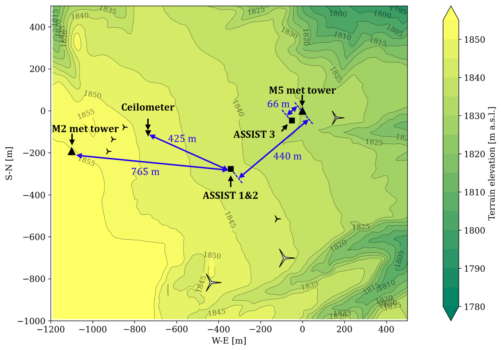
Figure 2 Map of the NLR Flatirons Campus in 2022. The size of the turbine rotors is to scale.

The climate at the site is typically semi-arid, with sunny conditions 70 % of the day, which generally produces a markedly diurnal cycle of atmospheric stability. Wind conditions are significantly affected by the diurnal cycle and by the presence of the Rocky Mountains to the west, which often channel the flow, creating strong winds (Hamilton and Debnath, 2019). The data collected by the M5 met tower confirmed these behaviors during the present campaign. In accordance with previous studies of the site (Aitken et al., 2014; Hamilton and Debnath, 2019), the atmospheric stability is classified based on the gradient Richardson number, Ri, evaluated between 3 and 122 m, using the ranges reported in Table 1. The hourly distribution of stability shows a clear daily cycle (Fig. 3a), also reflected in the daily averaged temperature (i.e., averaged every day at the same hour) signals at different heights above the ground (Fig. 3b). The wind rose is also shown in Fig. 3c.

Table 1 Stability classes based on the Richardson number calculated using 10 min-averaged temperatures and wind speed measured at 3 and 122 m.

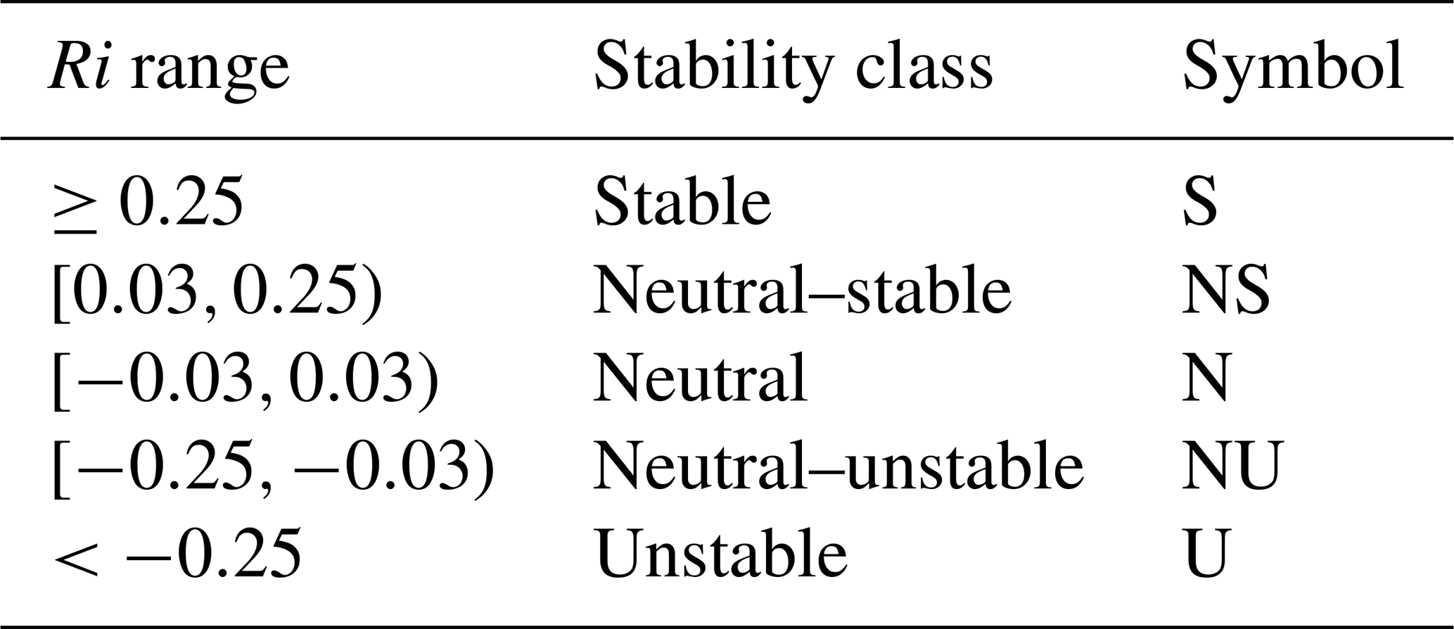
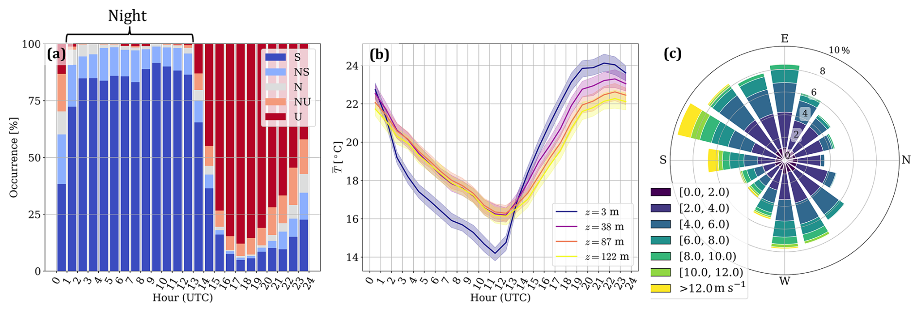
Figure 3 Climate statistics during the pre-AWAKEN campaign test from M5: occurrence of stability as a function of the time of day, based on the Richardson number between 3 and 122 m (S denotes stable, NS denotes neutral–stable, N denotes neutral, NU denotes neutral–unstable, U denotes unstable) (a). Daily averaged temperature at different heights, where the shaded region represents the 95 % confidence interval (b). Wind rose at 74 m (c). Precipitation and wake events are excluded.

Temperature profiles were retrieved using TROPoe v0.12 (Turner, 2026), which ingested the spectral radiance from the ASSIST at selected bands as the main observations. The prior used to facilitate the convergence of TROPoe includes ensemble means and level-to-level covariances of temperature and mixing ratio profiles from 1811 radiosonde launches in the Denver area. The lowest CBH from the ceilometer is also assimilated by TROPoe to enhance the accuracy of the solution in cloudy scenarios (Turner and Löhnert, 2014).

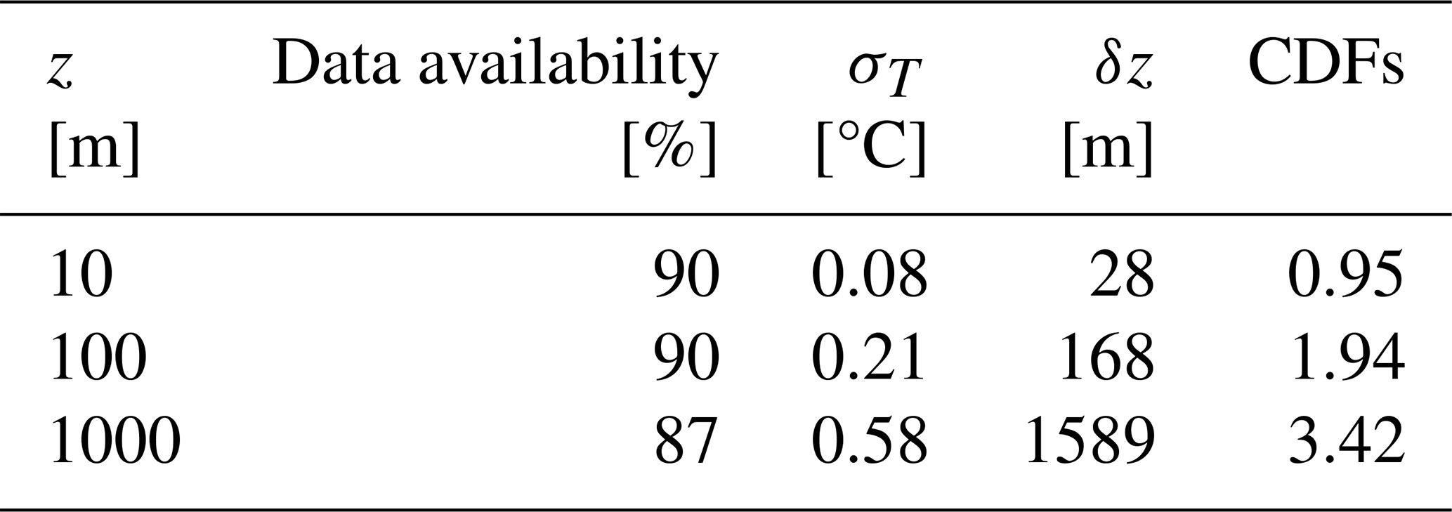
TROPoe profiles are quality-controlled by rejecting data above the base of optically thick clouds, with the root-mean-square (rms) between the observed and predicted radiance being larger than rms > 5 or with the convergence parameter being γ>1 (see Letizia et al., 2025, for details). Clouds detected when the TROPoe estimate for the liquid water path is less than 5 g m⁻² are considered to be optically thin and thus are bypassed. Table 2 reports the overall TROPoe temperature statistics for ASSIST 1 in terms of data availability after quality control, mean uncertainty (σ_T), mean vertical resolution (δz), and cumulative degrees of freedom (CDFs). The latter is a measure of the information content below the selected height (see Turner and Löhnert, 2014). Uncertainty and vertical resolution increase with height, while most of the information content is confined close to the surface. This is typical behavior of atmospheric sounding based on ground-based passive observations (Turner and Löhnert, 2021).

Table 2 Data availability; mean uncertainty, σ_T; and vertical resolution, δz, of TROPoe retrievals for ASSIST 1 based on 12 927 temperature profiles derived from data collected during the pre-campaign test.

Temperature profiles are generated every 10 min as a trade-off between temporal resolution and computational costs. To achieve this, TROPoe extracted the nearest-in-time spectral radiance collected by the ASSISTs at a sampling rate of ∼14 s. The radiative transfer model is non-linear, and so using high-frequency observation rather than, for instance, 10 min-averaged ones prevents the ingestion of non-realistic spectral radiances that can occur when averaging several sky scenes with different radiative properties. This is typical of scattered cloudy conditions. One drawback of using ASSIST data collected at the native sampling rate is that the noise is not averaged out as it would be when using time-averaged radiances. Therefore, the noise in the spectral radiances is removed through a principal component analysis filter (Turner et al., 2006).

Furthermore, the use of high-frequency data implies that the observed profiles include a significant turbulent contribution. To understand the behavior of turbulence at the site, we calculated the directional, daily averaged, 10 min second-order moments of both temperature and wind speed in the form of temperature standard deviation ($\sqrt{\stackrel{\mathrm{‾}}{T^{\prime ,\mathrm{2}}}}$) and turbulence intensity (TI) from 1 Hz met tower data (Fig. 4). The inner circle of the polar plot corresponds to nighttime, whereas the outer one corresponds to daytime. In other words, radial variations of the quantity indicate a diurnal cycle, and departures from axial symmetry represent the effects of wind direction. Both $\sqrt{\stackrel{\mathrm{‾}}{T^{\prime ,\mathrm{2}}}}$ and TI show the expected diurnal cycle, with larger fluctuations during the day (i.e., unstable conditions), although directional effects are also important. In particular, the temperature standard deviation plot at 3 m (Fig. 4a) reveals consistently large fluctuations during night hours, especially for western–southwestern winds. A TI peak for the same time and/or direction is not evident. The fluctuations occurred with periods of several minutes and were confined close to the surface, which is reminiscent of the gravity wave events documented by Sun et al. (2015). Further investigation is beyond the scope of this work; however, the effect of turbulent fluctuations on the temperature differences observed at different sites is discussed in Sect. 3.3.

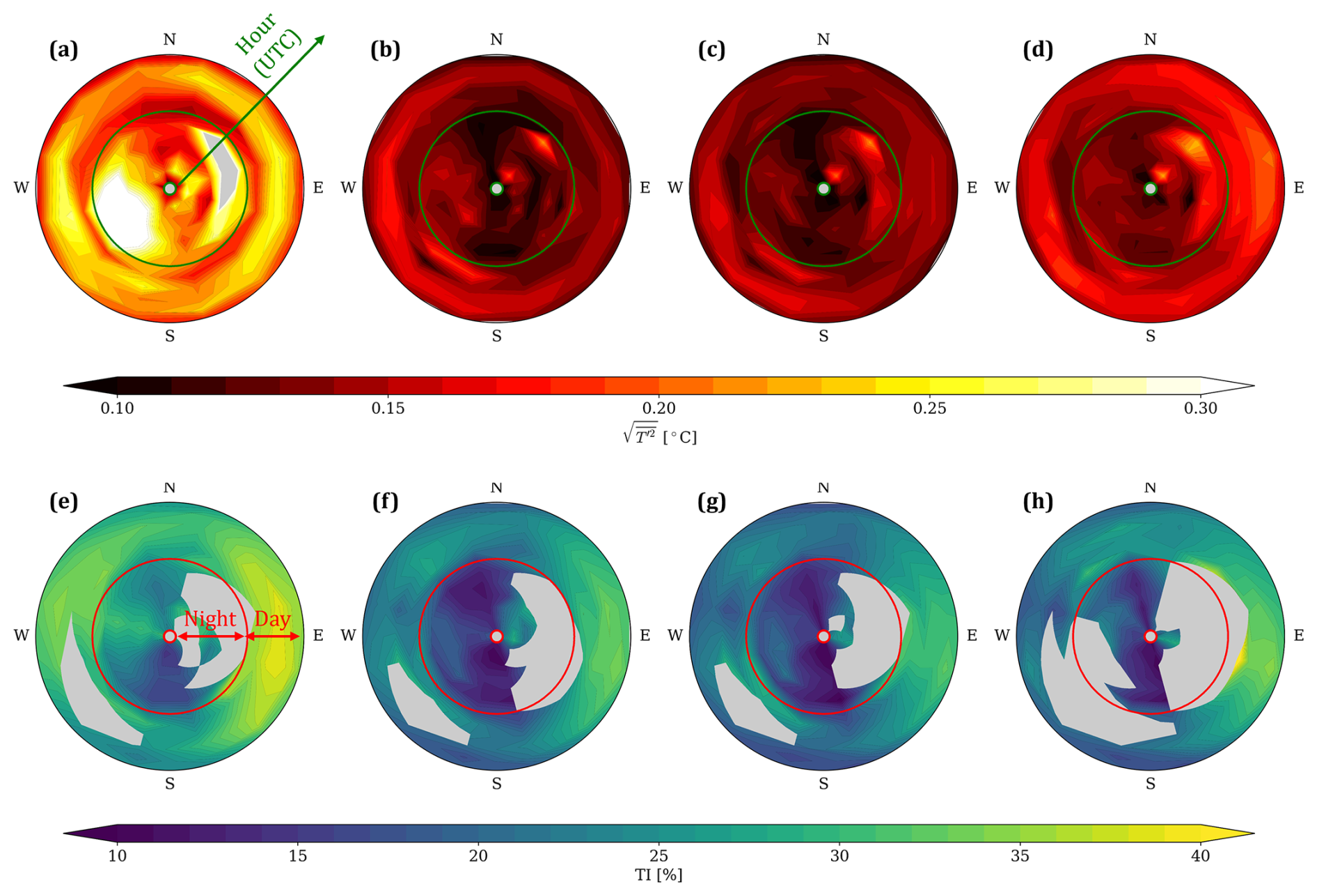
Figure 4 Directional, daily averaged standard deviation of temperature (a–d) and turbulence intensity (TI) (e–h) at different heights: 3 m (a, e), 38 m (b, f), 87 m (c, g), 122 m (d, h). The empty areas have a 95 % confidence interval larger than 0.1 °C or 10 % for temperature standard deviation and TI, respectively.

3.2 Exploring instrumental error: side-by-side test

In this section, we discuss the temperature differences observed between the co-located ASSIST 1 and 2. The comparison is important to assess the instrumental error. In fact, subtracting the temperature estimated by TROPoe for the two independent instruments leads to a theoretically perfect cancellation of the smoothing and radiative model errors in TROPoe. What is left is the effect of bias in the measurements (which would translate into a mean temperature difference) and noise (which would translate into a random, zero-mean temperature difference). By applying the general TROPoe posterior uncertainty (Eq. 1) to the temperature difference, we get the following:

$$\begin{array}{}\text{(2)}& \mathrm{\Delta }\widehat{T}={\widehat{T}}_{\mathrm{2}}-{\widehat{T}}_{\mathrm{1}}=\mathbf{G}({\mathit{ϵ}}_{\mathrm{2}}-{\mathit{ϵ}}_{\mathrm{1}}),\end{array}$$

where we have taken advantage of the equivalent TROPoe settings for both units to eliminate the smoothing error and isolate a common G matrix. Because instrumental noise, ϵ, is assumed to have zero mean, the theoretical mean of $\mathrm{\Delta }\widehat{T}$ is 0. We can safely assume negligible correlation between the instrumental noise of independent units so that the predicted covariance of the temperature differences is as follows:

$$\begin{array}{}\text{(3)}& S_{\mathrm{\Delta }\widehat{T}}=\mathbf{G}(S_{\mathit{ϵ},\mathrm{1}}+S_{\mathit{ϵ},\mathrm{2}}){\mathbf{G}}^{\mathrm{T}},\end{array}$$

where S_ϵ is the covariance of the instrumental noise for each instrument, a nearly diagonal matrix that is estimated by the ASSIST online. The instrument-to-instrument error standard deviation that we will use next, ${\mathit{\sigma }}_{\mathrm{\Delta }\widehat{T}}$, is then simply the square root of the diagonal $S_{\mathrm{\Delta }\widehat{T}}$.

To test the validity of this framework, we retrieved more than 10 000 temperature profiles through TROPoe from both ASSISTs and calculated statistics of the temperature difference, $\mathrm{\Delta }\widehat{T}$, at each height up to 2000 m above ground level. The results are shown in Fig. 5 in terms of the bias (i.e., mean difference) (a), rms of temperature difference (b), and probability of exceeding the 95 % TROPoe confidence interval (CI) predicted by TROPoe (c) as a function of height. The bias is extremely small (<0.02 °C) and practically irrelevant for most applications, which validates the assumption of negligible instrumental bias. The rms of $\mathrm{\Delta }\widehat{T}$ is below 0.3 °C and exhibits a gradual monotonic trend with height, except for a peak close to the surface; these bias and rms results agree with those of Turner et al. (2026). The error model based on TROPoe (${\mathit{\sigma }}_{\mathrm{\Delta }\widehat{T}}$ in Eq. 3 and the red line in the Fig. 5) is in fair agreement with the observations (black line). The trend as a function of height is well-captured, but the theory under-estimates the error below 100 m and overestimates it above this height. This discrepancy may arise from either an imperfect estimation of the noise from the ASSIST and/or noise that violates the assumption of Gaussianity used by TROPoe. To further explore the ability of theory to predict the distribution of $\mathrm{\Delta }\widehat{T}$, we plot the probability of $\mathrm{\Delta }\widehat{T}$ exceeding the 95 % CI obtained from Eq. (3) and assuming a Gaussian distribution (i.e., the probability that $\mathrm{\Delta }\widehat{T}\notin \pm \mathrm{1.96}{\mathit{\sigma }}_{\mathrm{\Delta }\widehat{T}}$). Close to the ground, where theory under-estimates the standard deviation of $\mathrm{\Delta }\widehat{T}$, there is up to 30 % probability of finding a value outside the CI, which is significantly larger than the expected 5 %. The corresponding real histogram (gray) and Gaussian fit (black line) of the probability density function (PDF) at z=10 m show a leptokurtic behavior of $\mathrm{\Delta }\widehat{T}$ not captured by TROPoe theory (red line), which always assumes Gaussianity. The model predicts fairly the bulk of variability around 0, but the likelihood of large and extreme $\mathrm{\Delta }\widehat{T}$ events is clearly under-predicted at this height. Moving to z=1000, we see an opposite behavior: the mean uncertainty estimation by Eq. (3) is too conservative, with real values being more tightly clustered around 0 than predicted. These opposite trends cancel out at z=100, where the prediction of TROPoe is spot on.

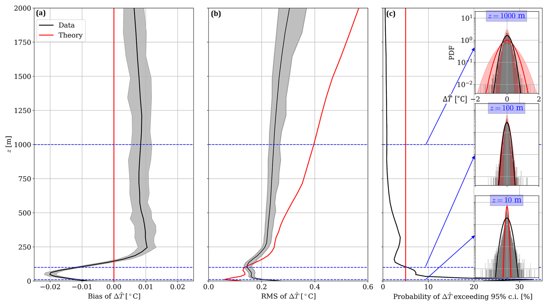
Figure 5 Vertical profiles of statistics of temperature differences between ASSISTs 1 and 2, $\mathrm{\Delta }\widehat{T}$: mean (a), rms (b), and probability of exceeding the 95 % TROPoe CI (c). The PDFs of temperature difference at selected heights are provided as insets with equal axes in (c). The shaded area in (a) and (b) represents the 95 % statistical CI, while that in (c) represents the PDFs with the largest and smallest TROPoe uncertainty. The red lines are the theoretical predictions.

The main takeaways of this section are as follows:

1. TROPoe temperature retrievals from two identical ASSISTs show negligible bias and an rms of <0.3 °C difference, with the latter being predicted fairly well by the TROPoe uncertainty product.

2. Random uncertainty from both the met data and TROPoe estimate spikes and departs from Gaussianity in the lowest 20 m, with TROPoe underpredicting its magnitude slightly.

3.3 Quantification of total error near the surface: comparison with met tower

Now that the instrument-to-instrument error has been documented and proven to be negligibly biased and predictable for common applications, in this section, we focus on a more comprehensive characterization of the total error. This includes contributions from the smoothing, forward model, and prior in addition to the error due to instrumental noise. The total error of the temperature profiles is quantified through a comparison with the temperature readings of the resistance temperature detector (RTD) platinum probes installed on the M5 tower. Specifically, the temperature profile is reconstructed by combining the absolute temperature measured by the RTD at 3 m and differential temperature measurements still from RTD pairs between 3 and 38, 38 and 87, and 87 and 122 m. The use of differential temperature measurement is advantageous because it maximizes the sensitivity of the probe, allowing the gain applied to the raw signal to be decreased and, thus, the error amplification to be reduced. Resulting temperatures at four heights (3, 38, 87, and 122 m) have a reported uncertainty of 0.1 °C (St. Martin et al., 2016), which we interpret as a 1σ value. Temperature probes are housed inside a radiation shield with active ventilation capabilities. However, during this campaign, some ventilation fans were not active. Therefore, the temperature readings from the unaspirated sensors on M5 were corrected for radiative error using the method by Nakamura and Mahrt (2005) and the M2 tower (which was aspirated) as a reference (see Appendix A for details).

The high-frequency temperature time series from M5 collected at 1 Hz are downsampled through a rolling average to match the sampling rate of the ASSIST (14 s) and then are linearly interpolated in time on the TROPoe time grid (one profile every 10 min). TROPoe data are interpolated linearly in z to match the met tower heights. No attempt is made to time shift either dataset to account for the advection across the 440 m distance between the two instruments, mainly because the dataset also encompasses wind sectors where the two instruments are not aligned with the wind. Differences in temperature due to the spatial decorrelation of turbulent thermal structures in space are, therefore, an additional source of random “representativeness” error in the data and will be discussed separately.

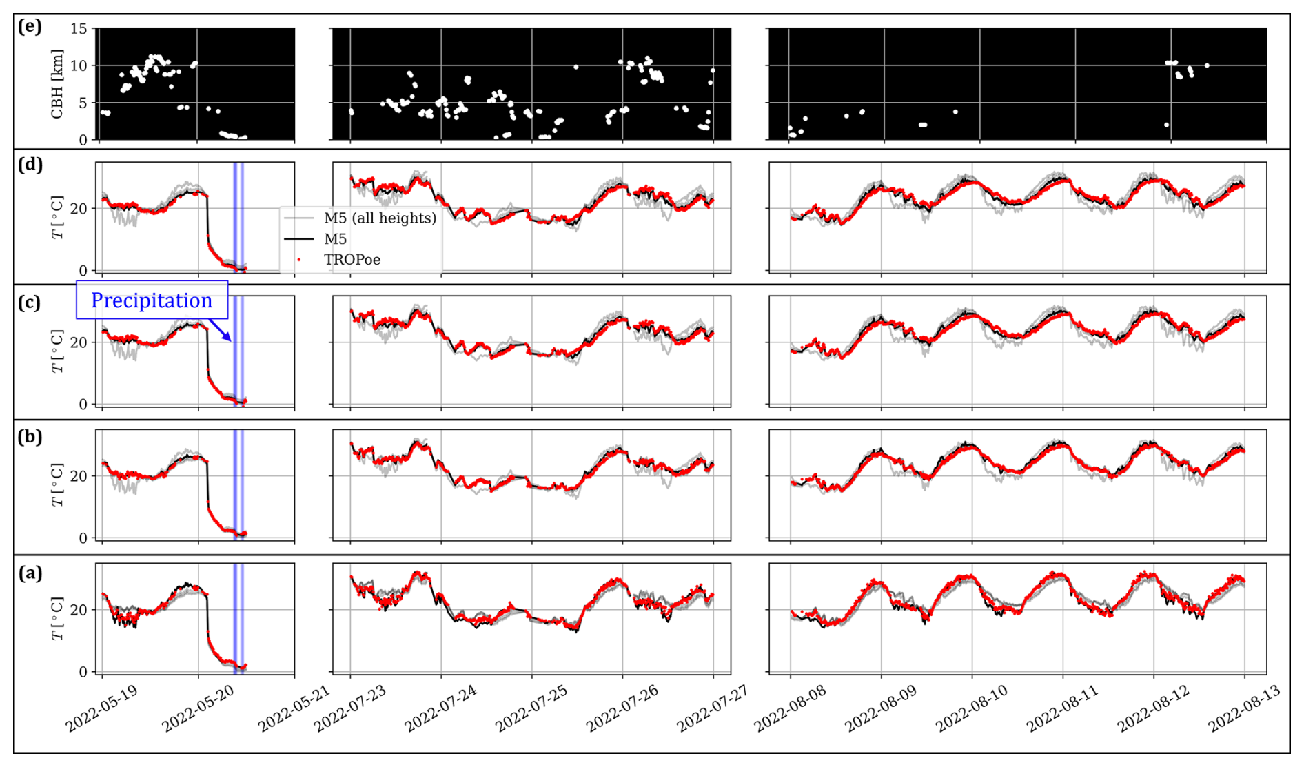
Figure 6 Selected time series of temperature from M5 and TROPoe at different heights: 3 m (a), 38 m (b), 87 m (c), and 122 m (d). The CBH is shown in (e). The light-gray lines represent the met tower observations at all heights and are superposed to evaluate the ability of TROPoe to match vertical temperature gradients.

Figure 6 shows three illustrative time series from both met probes and TROPoe at all available heights. The first was recorded during the passage of a cold front that caused a drop in temperature of about 15 °C in 20 min. TROPoe detects the drastic temperature change with excellent agreement when compared to M5, indicating the ability of our ground-based passive temperature profiling method to work robustly in dynamic atmospheric environments.

The second time series corresponds to an overcast event (see cloud height in the top panel) that disrupted the typical diurnal thermal cycle. Discrepancies during the coldest hours with low clouds are within a fraction of a degree. This is an early indication that temperature estimates close to the surface are minimally affected by clouds that, as we mentioned, represent a major challenge for temperature profiling using passive spectral infrared methods. The accuracy of TROPoe in this case is remarkable considering the fact that low clouds have a powerful emission in the infrared region that may have obscured the thermodynamic information.

The third and possibly more insightful time series corresponds to a sequence of hot, clear-sky days. Here, the differences between TROPoe and the met tower appear to be more systematic, with a consistent warm bias at night and a cold bias during the day, with the latter being less evident at the lowest height.

Figure 7 offers a more quantitative insight into the temperature differences over the entire dataset. Linear fits at different heights (Fig. 7a, b, c, d) show R² above 0.98; very small bias; rms <1 °C; and, interestingly, a slope of slightly less than 1 at all heights. Rather than being a statistical artifact (e.g., slope dilution; Frost and Thompson (2000)), this is more likely to be an indication that TROPoe is under-estimating either the diurnal variation of temperature compared to M5 or the effect of a residual error in the correction of the radiative error of M5 (see Appendix A). This feature is also consistent with the diurnal bias shown in Fig. 6.

Before digging into the possible cause of the observed discrepancies, an important question is as follows: how well does the TROPoe posterior uncertainty product capture the observed differences? To this aim, we visualize histograms of temperature differences at all heights (Fig. 7e, f, g, h) and superpose the expected error Gaussian PDF obtained by combining TROPoe–M5 uncertainties. The real PDF of ΔT (gray bars) is minimally biased and arguably Gaussian, especially above 3 m (the black line is the Gaussian fit). However, the standard deviation is 3 to 5 times larger than the predicted uncertainty, indicating an additional source of error in the dataset. Having excluded the instrumental bias or an under-predicted noise in Sect. 3.2, we are left with two main candidate sources of uncertainty: the spatial separation between the ASSIST location and M5 and the radiative transfer model (the prior was confirmed to match the observed climatology and thus was ruled out as a source of uncertainty).

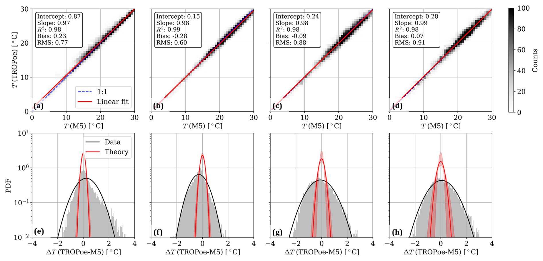
Figure 7 Statistical quantification of the temperature differences between TROPoe and M5 at different heights: (a–d) linear regression and (e–h) histograms, where the red-shaded area indicates the error PDF using the minimum and maximum combined TROPoe–M5 uncertainty. Heights are as follows: 3 m (a, e), 38 m (b, f), 87 m (c, g), and 122 m (d, h).

The error due to spatial separation is associated with the spatial decorrelation of turbulence. Its magnitude can be estimated through the temperature structure function, defined as the variance of the temperature difference as a function of space. For an ergodic, horizontally homogeneous field, this reads as follows:

$$\begin{array}{}\text{(4)}& D_T(\mathit{r},z)=\stackrel{\mathrm{‾}}{\left(T\right(\mathit{x})-T(\mathit{x}+\mathit{r}){)}^{\mathrm{2}}},\end{array}$$

where the overbar indicates the time average (in our case, over the standard 10 min window), r is the separation along a certain direction, and x is a reference point in space. A direct application of Eq. (4) would require the placement of multiple sensors at different locations. For the sake of simplicity, instead, it is customary to use Taylor's frozen-turbulence hypothesis (Taylor, 1938), which de Silva et al. (2015) showed to work well up to separation distances as large as the boundary layer height under neutral conditions. Han and Zhang (2022) showed that Taylor's hypothesis fails to replicate spatial-structure temperature functions under unstable conditions and for short separations, but it works well under other conditions. Here, we use Taylor's hypothesis to calculate the structure function based on temperature time series from the met tower up to separations of 440 m under all atmospheric conditions, which, based on the cited references, should represent an acceptable approximation of Eq. (4) for most of the cases. To maximize realism in the estimation of the spatial error between TROPoe and the met tower, we calculate the structure function of the temperature data downsampled to the ASSIST sampling rate of 14 s. Furthermore, we restrict the analysis to cases where the ASSIST and the met tower are aligned within 20° from the mean wind direction and to TI values smaller than 50 % (Stull, 1988).

Figure 8 shows the standard deviation of the temperature differences based on the (square-rooted) time-based structure function at different heights and stabilities. The choice to cluster data in this function is inspired by the classical scaling of structure functions (Wyngaard et al., 1971; Wyngaard, 1973), which relates this statistical parameter mainly to stability and height. The structure function is observed to generally decrease with height and increase under unstable conditions, where more turbulence is expected. In our dataset, it also increases moving from neutral to stable, which is likely to be connected to the nighttime temperature oscillations whose signature appears in Fig. 4.

In the same figure, we report the residual rms of the temperature difference between TROPoe vs. M5 after subtracting the known TROPoe–M5 uncertainty for ASSIST 1 (placed 440 m away from M5) and ASSIST 3 (placed 66 m away). If spatial variability were the only cause of the residual discrepancy, we would expect a match with the value estimated from the structure function at the corresponding distance, height, and stability. Although some trends do match (the highest rms values occur under stable and unstable conditions), the residual variability of ΔT far exceeds the estimated spatial component for most of the bins. An even stronger piece of evidence that the discrepancies between TROPoe and met are not only turbulence-driven is that the error does not decrease when moving from ASSIST 1 (440 m away) to ASSIST 3 (only 66 m away). The fact that some additional source of uncertainty other than turbulence is contributing to fattening the PDF of ΔT is also suggested by the cyclical (and, thus, not random as turbulence would be) difference observed in Fig. 6 for clear-sky conditions.

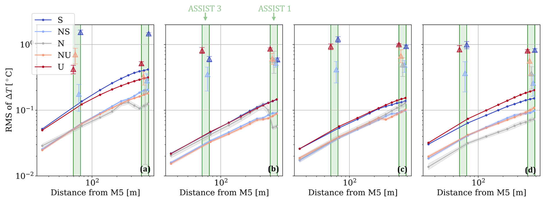
Figure 8 Estimated standard deviation due to spatial separation (lines) as a function of distance from M5 and stability at different heights and corresponding rms of temperature difference from ASSISTs 1 and 3 (triangles). Known TROPoe and met tower uncertainties were removed from the rms to isolate the residual component. Heights are as follows: 3 m (a), 38 m (b), 87 m (c), and 122 m (d).

After ruling out spatial variability as the only contributor to the temperature difference, we focus on describing the residual errors as a function of the atmospheric conditions. An objective way to assess the relevance of a set of inputs in describing a target parameter is the importance ranking through random forest permutations. We apply the framework described in Letizia et al. (2024) to the description of ΔT as a function of the atmospheric quantities in Fig. 9 for separate heights. The Richardson number (viz., stability) emerges as the most important parameter that describes the temperature differences. This confirms that the diurnal error pattern discussed earlier is ubiquitous in the dataset.

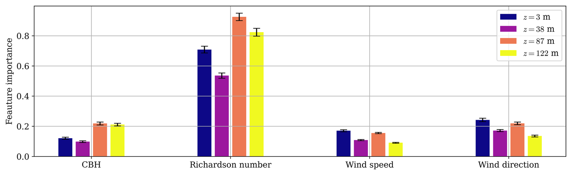
Figure 9 Random forest permutation feature importance of several atmospheric parameters as a descriptor of the temperature difference between TROPoe and M5.

To understand the magnitude of what appears to be a stability-dependent bias, we evaluate mean temperature profiles from TROPoe, M5, and M2 at the native heights for the different stability classes. Care is taken to ensure that only periods when all three sources are available are included. Figure 10 shows the mean profiles, along with their 95 % statistical CI. The stability-dependent bias between TROPoe and M5 is more severe at higher z and for unstable and stable conditions. Neutral and near-neutral conditions show a bias that is within the statistical uncertainty. Compelling evidence that the observed difference is an actual bias and not an instrumental error from the met sensors or the effect of persistent thermal inhomogeneity is the excellent agreement between M5 and M2. To sum up, the present analysis highlights a stability-dependent bias that is always less than 1 °C and is mostly positive under stable conditions (TROPoe warmer than met towers) and negative under unstable conditions (TROPoe colder than met towers, except very close to the ground). Differences in terms of this magnitude are similar to what has been reported by previous studies (Blumberg et al., 2015; Klein et al., 2015; Bianco et al., 2024).

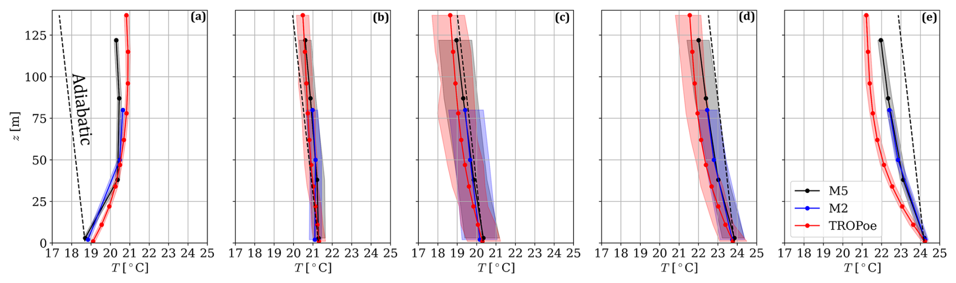
Figure 10 Mean temperature profiles for different stabilities: 6112 stable profiles (a), 862 neutral-stable profiles (b), 210 neutral profiles (c), 394 neutral-unstable profiles (d), and 3314 unstable profiles (e).

To conclude this section, we discuss the accuracy of temperature profiling in capturing vertical temperature gradients and, hence, the static stability of the surface layer. We first look at the linear regression between the vertical temperature gradient, ΔTΔz⁻¹, evaluated for M5 vs. TROPoe at height pairs (Fig. 11). The highest agreement is observed for the combination of heights that result in larger gradients (i.e., close to the ground or for large vertical spacing), with R² values of 0.88. The agreement is slightly worse than what was reported for the LABLE experiment (Klein et al., 2015), although that study only included temperature gradients in the ±0.01 °C m⁻¹ range and had a smaller distance between the thermodynamic profiler and the reference instrument (the radiosonde launch station was 300 m away from the spectrometer). Poorer scores occur for height combinations where ΔTΔz⁻¹ is small, which is expected for a constant level of random error or unexplained variance between the two variables. Also, at short vertical separations, the finite vertical resolution of the TROPoe grid begins to play a significant role.

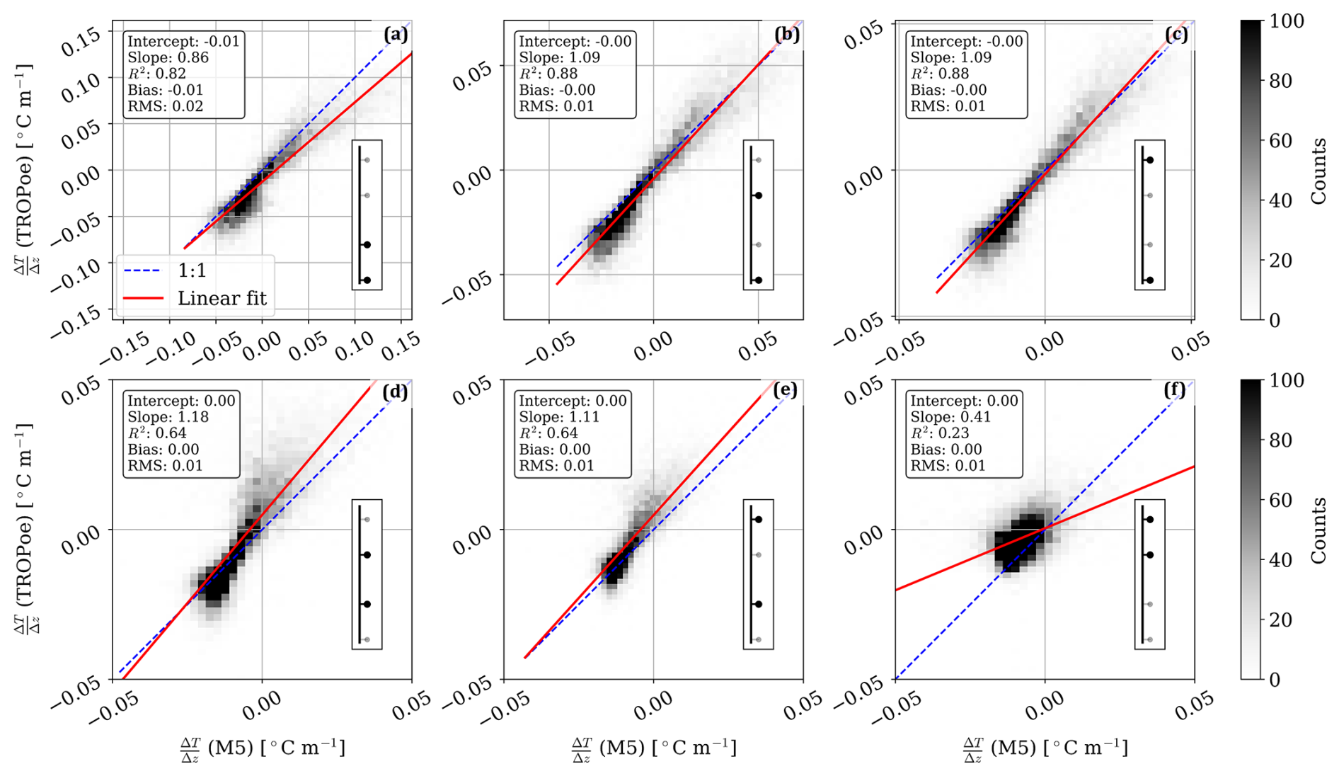
Figure 11 Linear regression between vertical temperature gradients from different height pairs: 3 and 38 m (a), 3 and 87 m (b), 3 and 122 m (c), 38 and 87 m (d), 38 and 122 m (e), and 87 and 122 m (f).

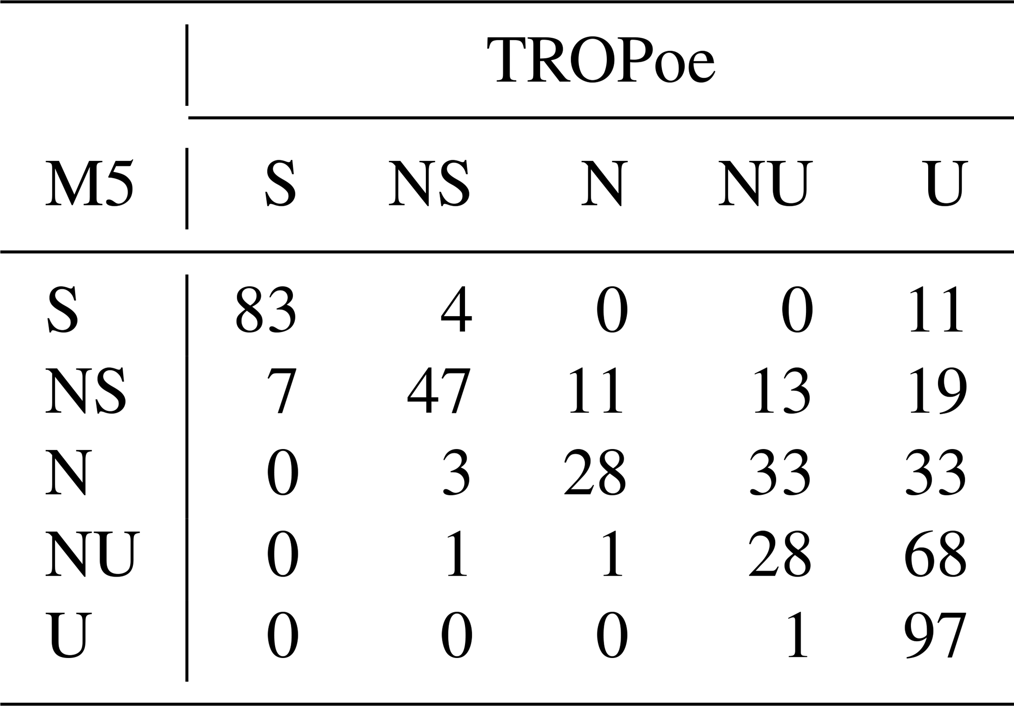
We finally assess the difference in Ri-based stability classification when using M5 vs. TROPoe data. The Richardson number from TROPoe uses temperature and moisture content from TROPoe itself, while wind gradients are still necessarily from M5. Table 3 shows, for each stability class defined from the Richardson number using M5 (rows), the percentage distribution of stability classes derived from the Richardson number using TROPoe (columns). Both Ri values are evaluated between 3 and 122 m. This contingency table shows good agreement for the stable and unstable classes (83 % and 97 % hits, respectively). More discrepancies are observed for neutral and near-neutral conditions. These classes are also the narrowest in terms of Ri range and constitute those with the lowest occurrence, thus making them more sensitive to differences in lapse rate. TROPoe exhibits an unstable bias compared to M5. For instance, 11 % of stable occurrences according to M5 are identified as unstable by TROPoe, which is consistent with the cold bias at 122 m shown in Fig. 10e. An imperfect removal of the overheating (Appendix A) due to solar radiation (the probe at 122 m is not aspirated) may also have contributed to the apparent unstable bias.

Table 3 Percentage contingency table of stability classification based on Richardson number from either M5 (rows) or TROPoe (columns).

The main takeaways of this section can be summarized as follows:

1. ASSIST–TROPoe performs satisfactorily at all of the heights and under all of the conditions we tested for what could be considered to be typical wind energy and meteorological applications, with an overall rms of temperature difference in relation to the met tower of less than 1 °C and negligible overall bias.

2. The rms of temperature differences could not be fully explained in terms of TROPoe and met tower uncertainty estimates and spatial decorrelation of thermal turbulence.

3. We identified a stability-dependent bias of less than 1 °C that deserves further investigation.

4. ASSIST–TROPoe is confirmed to be remarkably accurate in identifying the static stability of the surface layer, particularly for very stable and unstable conditions.

4 Results from AWAKEN

4.1 Overview

AWAKEN is a multi-institutional experimental campaign with the goal of investigating the interactions between the atmospheric boundary layer and land-based wind plants. It took place from 2023 to 2025 in northern Oklahoma in the United States. The reader is referred to Moriarty et al. (2024) and references therein for more details regarding the instrument layout and science goals.

Temperature profiling was an essential asset at AWAKEN and used the network of sensors shown in Fig. 12. This included three ASSISTs (“South”, “Middle”, and “North”), which were strategically placed to capture atmospheric conditions throughout the experimental domain. Each ASSIST was co-located with a surface met station (Goldberg, 2023e, f, g). Additional temperature profiling was conducted through radiosondes launched from the northernmost site (Keeler et al., 2023).

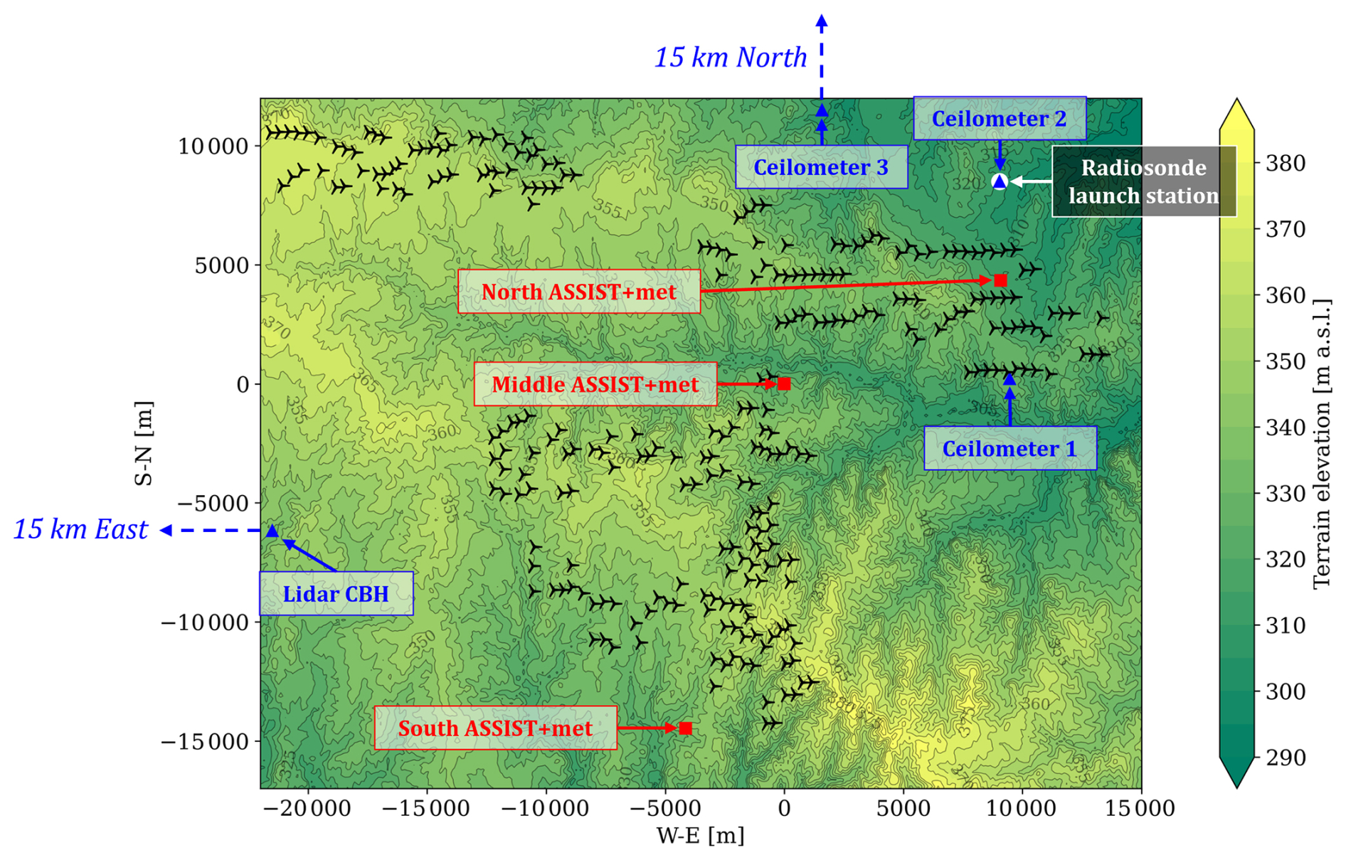
Figure 12 Map of the instruments used for temperature profiling and wind turbines at AWAKEN.

TROPoe was run with the same setup as that described in Sect. 3.1 and using a CBH from the three ceilometers (Hamilton, 2023; Zhang et al., 2023b, a) and including the lidar (Shippert et al., 2023), indicated on the map in blue. To account for the spatial variability of cloud cover, the CBH for each ASSIST site was estimated as the average CBH from all available sources weighted by the inverse of the respective distance. The data availability of all input instruments and TROPoe retrievals is shown in Fig. 13. Overall, roughly 1 year of temperature profiles is available from all of the sites combined.

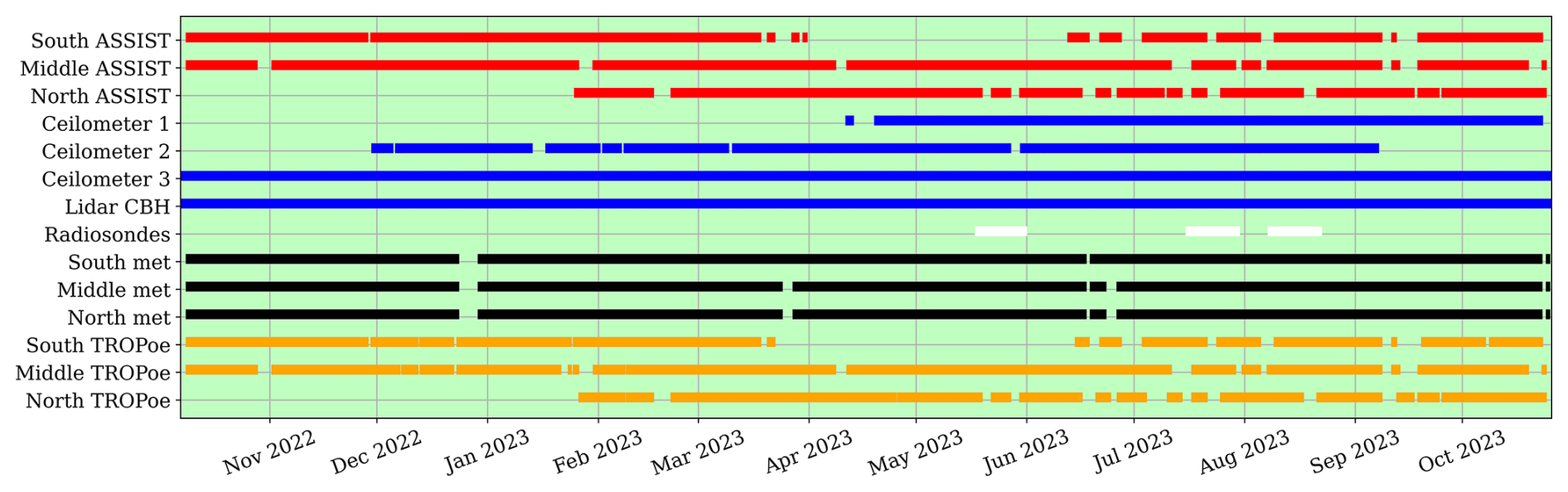
Figure 13 Timeline of the data availability in channels used for thermodynamic profiling at AWAKEN.

4.2 Quantification of error in the whole ABL: comparison with radiosondes

The goal of this section is to quantify TROPoe's total error and the accuracy of the uncertainty estimate across the ABL. To this aim, we compare TROPoe retrievals at the North site with observations from radiosondes at AWAKEN. Radiosondes were launched in different phases from 17 May to 22 August 2023 at site H. The radiosonde model is the Vaisala RS-90, with an accuracy of temperature measurement of 0.15 °C (Holdridge, 2020). The nominal schedule included five launches at 02:30, 05:30, 08:30, 11:30, and 23:30 UTC, aimed at probing the nocturnal ABL. Out of the 198 available radiosonde launches, 116 have concurrent TROPoe retrievals and are used in this analysis. The comparison is carried out in comparison to radiosonde profiles downsampled at the ASSISTs sampling rate (14 s), both at the native resolution vertical and at a “TROPoe-smoothed” resolution, as done by Blumberg et al. (2017). It can be proven (Letizia et al., 2025) that smoothing high-resolution profiles using the TROPoe averaging kernel and prior theoretically eliminates the smoothing error and isolates the noise contribution.

All profiles and error statistics are shown in Fig. 14. The bias (Fig. 14a) peaks at the surface, where it reaches the modest value of 0.2 °C, which is smaller than what was reported in previous similar studies (Blumberg et al., 2015; Klein et al., 2015; Blumberg et al., 2017; Turner and Blumberg, 2019; Turner and Löhnert, 2021). By looking at the temperature difference map in Fig. 14e, it appears to be the case that the cold bias close to the surface is due to persistent patches of negative temperature differences in the lowest 100 m associated with positive difference aloft that occurred for specific launches. Finally, smoothing the radiosonde profiles has little impact on bias.

The rms of temperature difference (continuous black line in Fig. 14b) shows a peak at the surface (0.9 °C) and a monotonic positive trend above 100 m. Values of the rms in the range of heights considered are in line with several references (Blumberg et al., 2015; Klein et al., 2015; Turner and Blumberg, 2019), except for the high value at the surface. This high rms close to the ground is also due to the bias just discussed. The TROPoe total uncertainty estimate (continuous red line in Fig. 14b) amplified with the radiosonde (small) uncertainty captures the trend of rms above 100 m remarkably well, although with an average 20 % under-estimation. This under-estimation may be due to the effect of spatial decorrelation at the distance between the two instruments (4 km at the ground). The rms difference with smoothed radiosonde profiles (dashed black line in Fig. 14b) is expectedly lower than the total rms due to the removal of the smoothing error, with TROPoe's noise-only–radiosonde uncertainty estimate being off by 40 %, in part due to the persistent bias, which is not smoothed out.

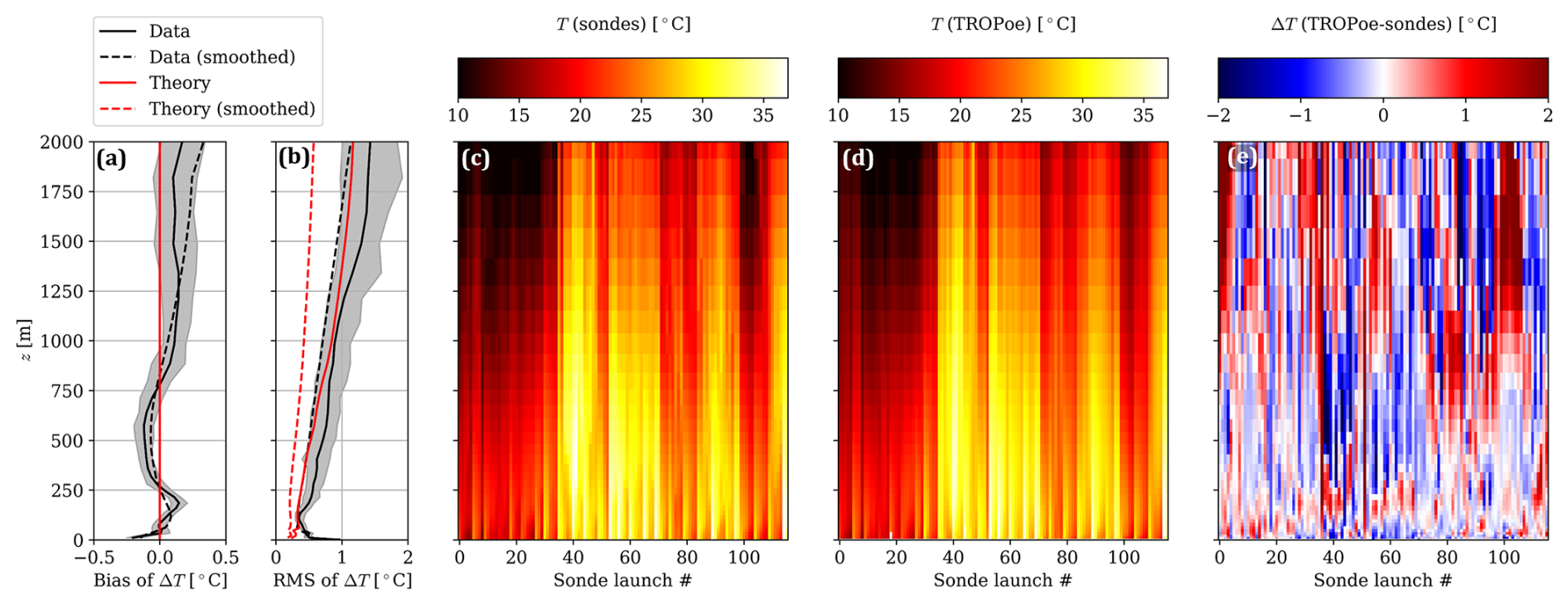
Figure 14 Vertical profiles of mean (a) and rms (b) of temperature differences between TROPoe at the North site and radiosondes, ΔT; all temperature profiles from radiosondes; (c) all temperature profiles from TROPoe at the North site (d); all temperature differences (e). Shaded areas in (a) and (b) correspond to the 95 % CI of the statistics for un-smoothed profiles.

The presence of a persistent temperature anomaly at heights where wind turbines operate at AWAKEN led to the hypothesis that the observed bias could be caused by wake effects. Turbine wakes are known to generate turbulence that warms up the air below the rotor height and cools down the region above it (Wu et al., 2023) by diminishing the lapse rate under stable conditions. What is shown in Fig. 14e, especially for launches 25 to 75, is compatible with wake effects affecting the radiosonde disproportionally more. The launch site is indeed downstream of the site where the North ASSIST operates (based on the prevalent wind direction) and, therefore, is in the wake of more turbines.

Early evidence that wake effects may have played a role in the observed temperature differences is provided in Fig. 15, which shows the temperature difference of TROPoe–sondes averaged from the ground to wind turbine hub height as a function of mean wind direction and wind speed in the turbine layer. The sign of the temperature difference is highly dependent on wind direction, with negative values occurring mostly for southern–southwestern winds and positive values for southeastern winds. Even if the complexity of the wind plant layout around both sites does not allow for an easy estimate of wake effects, the directionality of the temperature difference is a strong indication that site-specific conditions (wakes or terrain), rather than instrumental or TROPoe errors, are causing the bias.

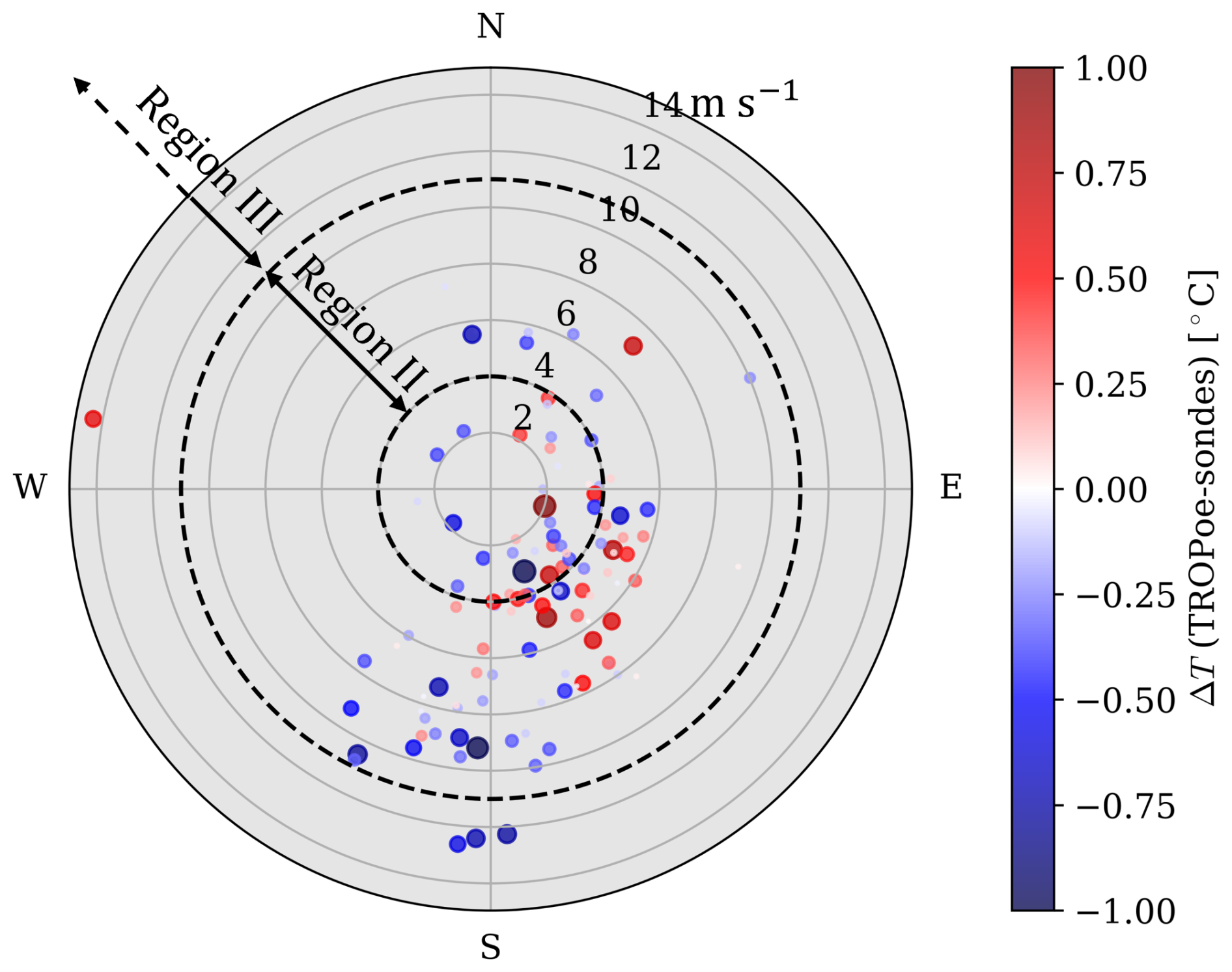
Figure 15 Mean temperature difference of TROPoe–sondes below hub height as a function of wind direction and wind speed in the turbine layer. The regions of the turbine power curve are also marked.

We can summarize the main results of this section as follows:

1. Temperature profiles are negligibly biased compared to radiosondes, and the random uncertainty is predicted fairly well by TROPoe.

2. Persistent temperature differences compatible with terrain or wake effects in the lowest 200 m contributed to increasing the rms of temperature differences close to the ground.

4.3 Ability to capture spatial gradients: comparison with surface met sensors

At AWAKEN, each ASSIST was co-located with a surface met station, which offers a unique opportunity to quantify the ability of temperature profiles to capture spatial gradients of temperature near the ground. For this comparison, we use temperature data collected by HMP45C Vaisala platinum resistance temperature detectors installed at 2 m above the ground level. The sensors have an average 1σ uncertainty of 0.25 °C (Campbell Scientific, 2007) and are shielded but not actively ventilated. We did not apply any correction for the radiative bias due to the absence of a reliable reference sensor.

The met data are provided natively as a 1 min average, which is a slower response than that of the ASSIST, and so what is shown next will include some representativeness error due to the different sampling rates. First, we characterize the difference between the met and TROPoe output interpolated to 2 m at the same site. The comparison is shown in Fig. 16. The agreement is excellent, with an R² of 1 to double-digit precision. The slope is consistently less than 1, similar to what we found in the pre-campaign test (Fig. 7). Diurnal overheating of the met sensors could also have contributed to reducing the slope. Positive biases of about half a degree are observed at the South and Middle sites. The North site is practically unbiased but shows slightly more scattering, possibly due to its proximity to the turbines, which may result in increased turbulence levels. The same ASSIST installed at the South site showed a much smaller bias in relation to the M5 met tower the year prior (Sect. 3.2). These South and Middle ASSISTs were also the same units used for the side-by-side comparison (Sect. 3.2), where they showed a negligible bias between each other. Given the pre-campaign results and the fact that the met and ASSIST were co-located at AWAKEN, we speculate that there may be ∼0.5 °C bias in some met sensors. The histograms of temperature differences (Fig. 16, bottom) suggest that the warm bias at the South and Middle sites is pretty consistent and not due to isolated outliers. It also proves that the uncertainty estimate of TROPoe–met agrees well with the variability noted in the observations (TROPoe uncertainty was, on average, larger at AWAKEN than in the pre-campaign test, mostly due to the different climatologies).

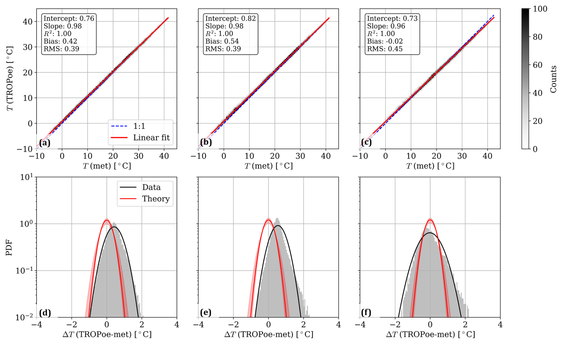
Figure 16 Statistical quantification of the temperature differences between TROPoe and met stations at the same site at 2 m: (a–c) linear regression; (d–f) histograms, where the red-shaded area indicates the error PDF using the minimum and maximum combined TROPoe–M5 uncertainty. South site (a, d), Middle site (b, e), and North (c, f). site.

After assessing that TROPoe performs remarkably well in capturing both the surface temperature and its uncertainty at AWAKEN, we move to a more challenging task: quantifying site-to-site temperature gradients. In fact, being a smaller quantity than the absolute temperature, it is more sensitive to inaccuracies. Figure 17 shows the comparison of the temperature differences from one site to the other as observed through TROPoe and the met. The linear regression shows expectedly poorer metrics compared to the previous comparison of absolute temperatures, but the agreement remains good. TROPoe can explain between 67 % and 86 % of the spatial variability of temperature, which is remarkable considering the fact that temperature differences hardly exceed 2 °C and that detection is done at a relatively high sampling rate (14 s). The agreement of the predicted uncertainty in the site-to-site gradient, Δ(ΔT), as shown in Fig. 17d–f, is also satisfactory. The previously observed bias at the South and Middle sites is canceled out in Fig. 17c but contributes to shifting the peak of the PDF in the other cases. The differences between the two instruments are, nevertheless, predicted well by TROPoe–met uncertainty at all sites.

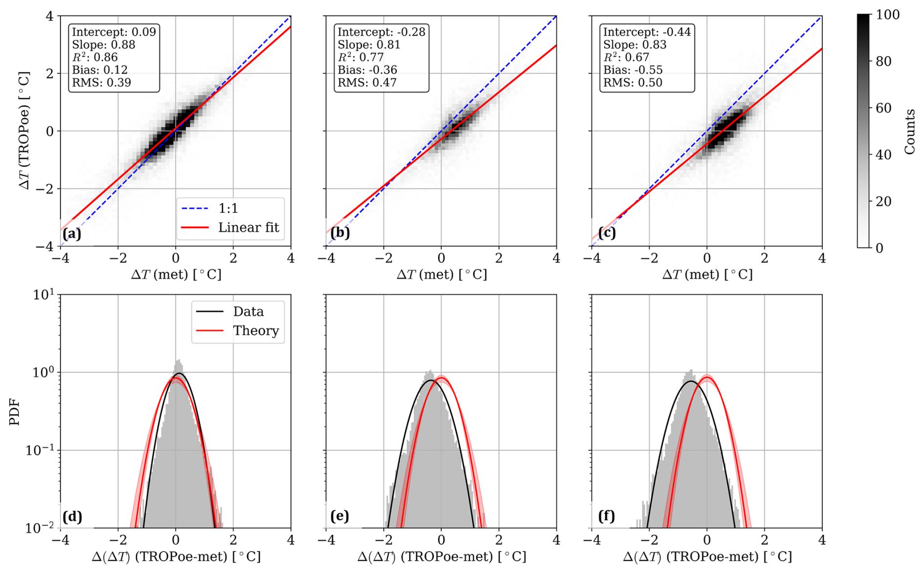
Figure 17 Statistical quantification of the differences between the site-to-site temperature gradients from TROPoe and met stations at 2 m: linear regression (a–c); histograms (d–f), where the red-shaded area indicates the error PDF using the minimum and maximum combined TROPoe–M5 uncertainty. Middle–South (a, d), North–South (b, e), and North–Middle (c, f).

Finally, to check if biases are still dependent on stability as we documented in the pre-campaign test, we calculate the mean temperature difference at the same site, ΔT, and the difference in terms of the site-to-site gradient, Δ(ΔT), for five stability classes. Stability classes are based on the Obukhov length detected by sonics at the nearby sites A2 and A5 (Pekour, 2022a, b) and using the table proposed by Krishnamurthy et al. (2021). As shown in the violin plots in Fig. 18a–c, the differences in absolute temperature do have a mild dependence on stability: the more stable, the warmer the bias in TROPoe vs. met, which is consistent with the pre-campaign results. This dependence is not present when looking at the differences in terms of site-to-site gradients (Fig. 18d–f). This seems to indicate that stability-driven biases in temperature profiles are consistent among different instruments and are canceled out when taking the difference.

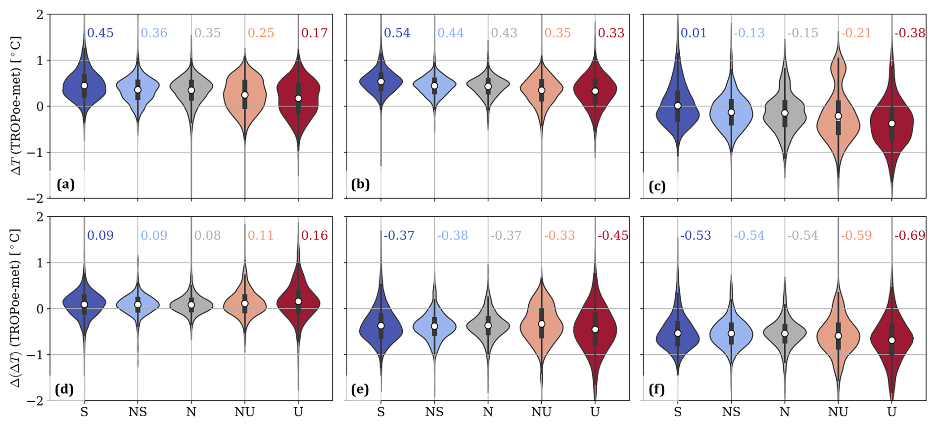
Figure 18 Violin plot of the difference in temperature (a–c) and site-to-site gradient (d–f) between TROPoe and met stations at 2 m for different stabilities: South site (a), Middle site (b), North site (c), Middle–South (d), North–South (e), North–Middle (f). The white dot and the number are the mean value, while the box spans the interquartile range.

To conclude the analysis of the AWAKEN dataset and to showcase the capabilities of the network of thermodynamic profilers in capturing relevant atmospheric phenomena, we take a close look at an interesting gravity wave event. The wave was likely to be the result of a bore generated by a thunderstorm located northwest of the AWAKEN site, which created gravity waves that traveled across the instrumented domain on 5 August 2023, from 10:40 to 11:20 UTC (just before sunrise). The event was detected by several permanent weather stations (National Weather Service, 2023; Newsom et al., 2023). The signature of the gravity wave appears most clearly in the reflectivity map of the weather radar in Vance, Oklahoma (National Weather Service, 2023). Snapshots of radar reflectivity are shown in Fig. 19, along with corresponding surface temperatures from all AWAKEN met stations (Goldberg, 2023a, b, c, d, e, f, g). We observe an increase in temperature at all sites during the passage of the bore, followed by a drop after 11:18 UTC as the cold air associated with the storm moves in.

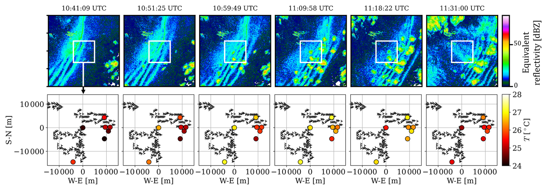
Figure 19 Snapshots of radar reflectivity and corresponding surface temperature from met stations during the wave passage on 5 August 2023.

The temperature overshoot is poorly understood when relying solely on surface temperature observations. The picture becomes much clearer when we include the temperature profiles (Fig. 20). We can readily identify a stably stratified surface layer before 10:50 UTC that is suddenly disrupted as the bore quickly passes through. The disruption takes the form of an initial surface warming, whereas the layers of air aloft rapidly cool down. The warming event occurs first at the South and Middle site and then at the North site about 10 min later, which is consistent with the west–east travel direction of the bore. After 11:20 UTC, the entire boundary layer at all sites eventually experiences the cold air. This is similar to a bore event observed by Haghi et al. (2019) using an AERI system. Another publication based on near-surface observations showed that nocturnal warming events associated with synoptic-scale cold fronts are common in Oklahoma (Nallapareddy et al., 2011). In our case study, we are likely to be observing a similar phenomenon but as a result of a thunderstorm outflow.

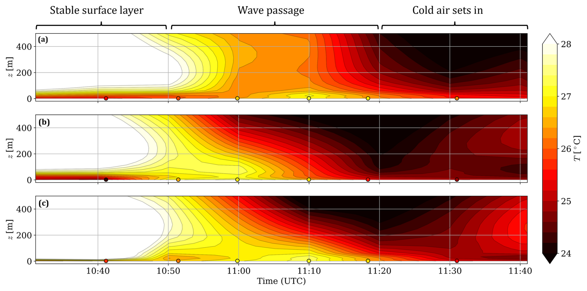
Figure 20 Time–height temperature maps from TROPoe at AWAKEN during a frontal passage on 5 August 2023: North site (a), Middle site (b), South site (c). The dots are colored according to the temperature from the met station at the respective site.

To summarize, in this section, we learned the following:

1. ASSIST–TROPoe temperatures agree extremely well with the measurements from surface stations at AWAKEN, with a nearly perfect R² and a bias of <0.5 °C, which is mostly site-dependent and weakly proportional to stability.

2. The TROPoe uncertainty estimate describes the observed differences in relation to the met stations well.

3. The network of thermodynamic profilers at AWAKEN are reliable tools for describing spatial gradients of temperature.

5 Conclusions

We documented the accuracy of temperature profiling methods used at AWAKEN through a four-stage validation exercise. We focused on temperature profiles obtained through the physical retrieval algorithm TROPoe and based on spectral radiance observations of ASSIST passive spectrometers.

First, we compared the difference in terms of temperature profiles between two thermodynamic profilers sitting side by side. The bias is negligible, and the random error is fairly predicted by TROPoe theory, except very close to the ground, where the tails of the temperature difference distributions are under-predicted.

Second, we assessed the difference between temperature profiles from one thermodynamic profiler and a nearby met mast up to 122 m above the ground. We saw an excellent agreement (R²>0.98, negligible bias, and rms difference of less than 1 °C). However, the temperature differences could not be explained solely by the sum of the TROPoe uncertainty estimate, the met sensors' nominal uncertainty, and the spatial decorrelation of thermal turbulence. Indeed, we identified a <1 °C stability-dependent bias whose analysis will be the subject of future work. We also verified the ability of temperature profiles to classify the static stability of the lower ABL, finding 83 % and 97 % hits for stable and unstable conditions, respectively.

Third, we compared temperature profiles at AWAKEN with 100+ radiosonde observations, reporting a <0.2 °C bias below 2000 m and an rms that follows the TROPoe prediction quite satisfactorily and never exceeds 1 °C below 1000 m.

Finally, we compared the site-to-site temperature gradients at AWAKEN from temperature profiles and the surface met station, finding a remarkable accuracy (R² between 0.67 and 0.86, bias of 0.5 °C, and rms well predicted by TROPoe) even for those small quantities.

In general, we confirmed that the combination of passive infrared spectrometers and physical retrievals allows for a fast, cost-effective, unsupervised, and continuous thermodynamic scanning of the lower atmosphere with traceable uncertainty. These results advocate for a wider use of this temperature profiling technique for wind energy and meteorology applications. Researchers will continue to improve the accuracy of temperature profiling to further reduce or explain the small but detectable differences with met tower observations. Future development efforts will also focus on making temperature profiling computationally and logistically less expensive, as well as expanding the data product to gas concentration profiles and cloud properties.

Appendix A: Correction of radiative error in temperature sensors

Lack of aspiration in the temperature sensors is known to cause overheating, especially under conditions of high solar radiation and low wind speed (Huwald et al., 2009). During the pre-campaign tests, the temperature sensors on M5 at the heights of 38, 87, and 122 m suffered from a failure in the aspiration system. However, temperature sensors on the M2 tower had operational ventilators for the duration of the experiment. Given the homogeneity of thermal conditions at the site, the average temperature difference between M5 and M2 was used as a proxy for the overheating due to solar radiation. This error has been subsequently corrected using the method proposed by Nakamura and Mahrt (2005) and tuned for the present site conditions.

First, the presence of radiative overheating was assessed by calculating mean temperature differences (interpolated) at 38 m as a function of global horizontal irradiance (GHI) and mean horizontal wind speed ($\stackrel{\mathrm{‾}}{U}$). The trends of the mean temperature differences, $\mathrm{\Delta }\stackrel{\mathrm{‾}}{T}$ (M5–M2), are shown in Fig. A1a. For GHI > 0 (daytime), there is a statistically significantly higher temperature at M5, which increases for low wind speed. This higher temperature is consistent with the presence of radiative overheating at M5. Interestingly, the highest temperature differences occur for moderate rather than high GHI. We speculate that, for high GHI, natural convection (not captured in the mean horizontal wind speed) may have contributed to cooling down the sensors. Negative GHI (nighttime) conditions also show a slight warming that could not be explained.

As suggested by Nakamura and Mahrt (2005), we estimate the overheating as a function of the following scaling parameter:

$$\begin{array}{}\text{(A1)}& X={\displaystyle \frac{\text{GHI}}{\mathit{\rho }{c}_p\stackrel{\mathrm{‾}}{T}\stackrel{\mathrm{‾}}{U}}},\end{array}$$

where ρ and c_p are the mean density and specific heat capacity of dry air. This quantity represents the ratio of radiative heating by the sun to the convective cooling by the wind. Figure A1b shows the 10 min and binned mean temperature difference vs. the scaling parameter and the associated linear fit. The slope of the linear fit is fairly close to the one provided in the original paper (434.76 vs. 373.40), hinting at similar heat transfer physics between the M5 sensors and those of Nakamura and Mahrt (2005). Still, the linear fit could explain only 32 % of the variance in the data, which suggests that other effects may have played a role (e.g., wind direction, spatial inhomogeneity). The linear correction in Fig. A1b based on 10 min averaged temperatures, wind speed, and GHI was applied to all M5 data and contributed to an average ∼0.2 °C drop in peak daytime temperature and a ∼10 %–15 % reduction in the rms of the temperature difference between TROPoe and M5.

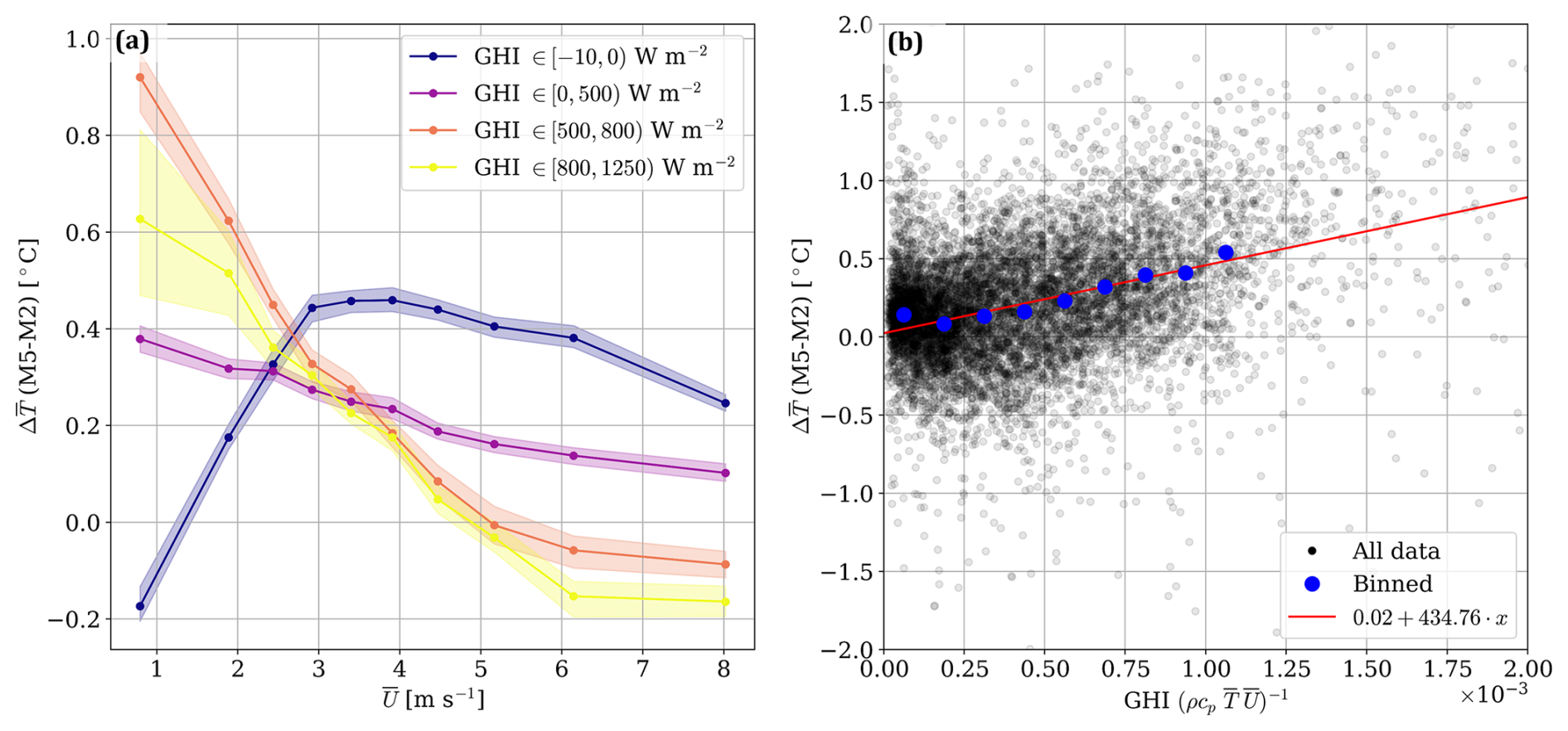
Figure A1 Summary of the aspiration correction: mean temperature difference (M5 − M2) at 38 m for different global horizontal irradiances and mean horizontal wind speeds, where the shaded area represents the 95 % CI (a), and linear fit of radiative error vs. overheating scaling parameter (b).