Lidar-enhanced closed-loop active helix approach

The helix approach has shown potential in increasing wind farm power production through enhancing wake mixing. By applying periodic blade pitch signals to upstream turbines, a helical wake is generated, which reduces velocity deficits for downstream turbines and mitigates the wake effect. While promising, the closed-loop implementation of the helix approach remains largely unexplored, which could enable handling uncertainties and model errors in wind farm applications. This work presents a framework that integrates lidar-based wake measurements to enable such closed-loop control. First, a downwind-facing continuous-wave lidar is used to extract the hub vortex as the controlled variable. Second, we developed a control algorithm that regulates the hub vortex position in the helix frame, thereby controlling the helical wake. Simulations in QBlade show that the framework enables a real-time, flow-informed closed-loop wake mixing approach. Compared with the open-loop cases, the framework corrects the shear-induced steady-state wake bias and enables measurement-informed, dynamic pitch adjustments under turbulence. In shear, bias correction increases downstream power but raises structural loads on both turbines; under turbulence, dynamic pitch control delivers a modest farm-level power gain with only minor load increases. These outcomes highlight the promise of flow-informed, closed-loop wake-mixing control and motivate further investigation.

1 Introduction

Wind energy plays a key role in mitigating climate change and achieving energy sustainability. However, in a wind farm, aerodynamic interactions between turbines reduce power production, increase structural loading and maintenance, shorten the lifetime of downstream turbines, and ultimately increase the levelized cost of energy (Houck, 2022). This interaction is called the “wake effect”, referring to the reduced wind speed and increased turbulence intensity that the downstream turbine experiences because of the upstream turbines' wake.

To mitigate the negative influences of wakes on the downstream turbines, some research aims at arranging wind turbines more effectively (Kusiak and Song, 2010), while other studies are working on control methods to get the best performance out of wind farms. These control approaches, known as wind farm flow control strategies (WFFCs), involve the coordinated control of individual turbines to actively manipulate the wake flow. The objective is to enhance overall performance metrics of the wind farm, such as total power output, system lifespan, or levelized cost of energy (Meyers et al., 2022). In general, three categories of solutions have been proposed, such as the axial induction control method proposed by Annoni et al. (2016), which involves deliberately operating the upstream turbine at less than its maximum capacity, with the aim of leaving more energy in the wake for downstream turbines. However, the potential for increased energy extraction from static induction control is rather low, making this method more suitable for load balancing within wind farms rather than overall production optimization (van der Hoek et al., 2019).

An alternative solution is wake steering, which refers to diverting the wake flow to mitigate the impact of the wake effect experienced by turbines downstream through yawing or tilting the upstream turbines. The redirected wake diverges from its initial path, decreasing its overlap with the rotor of a downstream turbine. As a result, the downstream rotor encounters higher speed and less turbulent wind, which can lead to an increase in power generation.

A different approach is suggested by Goit and Meyers (2015), where the wake is reduced by enhancing the mixing of the wake with the ambient free-stream air through dynamic variation of the induction. By promoting such mixing, the wake recovers energy more rapidly than through natural recovery alone. One implementation of this method is done by pitching periodically, hence creating a periodic structure in the wake; see Frederik et al. (2020b). Due to the periodic structure, this approach is more commonly referred to as the pulse approach. While this technique demonstrates substantial power gains in a two-turbine setup, it also leads to significant load increases due to variations in thrust force (Frederik and van Wingerden, 2022). Consequently, an alternative actuation method is proposed by Frederik et al. (2020a), where the position of the thrust force is rotated around its nominal axis rather than varying its magnitude. This generates a helical pattern in the wake, from which the approach derives its name as the helix approach. This approach significantly reduces power fluctuations while also achieving better overall performance than the pulse approach. The helix approach has attracted growing interest in the field, supported by large-eddy simulations (LESs) and wind tunnel experiments (van der Hoek et al., 2024), both demonstrating promising power gains.

Currently, the helix approach is implemented in an open-loop configuration, offering the advantage of being fast and easy to implement. However, the absence of feedback information regarding the output wake limits the system's ability to dynamically adjust control strategies in the presence of uncertainties and model errors. For instance, a constant bias in the output may arise from external wind conditions or unmodeled system dynamics. Robust feedback control can address these challenges by accommodating these uncertainties in wind energy production (Meyers et al., 2022). Enabling such control requires the measurement of the output, namely, the wake, which, from a control perspective, corresponds to integrating a feedback mechanism into the control architecture. To access the wake information generated from the upstream turbine, the current work of Kerssemakers (2022) has investigated the use of blade root bending moments from the downstream turbine. Our work explores an alternative way to integrate wake measurement into control by using light detection and ranging (lidar) sensing technology. When positioned downwind, a lidar can capture the wake generated by the upstream turbine, providing real-time feedback that enables the implementation of effective closed-loop control strategies. The work of Raach et al. (2017) utilizes this approach for closed-loop wake steering control, where a nacelle-based lidar system facing downwind is used to estimate the wake center and a control system is designed to steer the wake into a desired position. Simulation result shows an approximately 4.5 % increase in total power output for a two-turbine wind farm compared to the open-loop approach (Raach et al., 2016).

To the best of the authors' knowledge, closed-loop wake mixing control based on lidar measurements remains unexplored. Inspired by the work of Raach et al. (2017), this paper aims to develop and implement a closed-loop wake mixing framework. Among the two current wake mixing methods, this paper focuses on the helix approach due to the better mixing and reduced tower loads and power fluctuations (Frederik et al., 2020a). In summary, the following contributions are presented in this work:

1. We found an aerodynamic feature within the helical wake that exhibits a strong correlation with the wake dynamics and can be used for closed-loop wake mixing control.

2. We design and implement a framework, consisting of lidar and control subsystems, for the helix approach, achieving a flow-informed closed-loop implementation.

3. We evaluate (2) in a two-turbine setup in a free-vortex simulation platform (QBlade) simulation and compare it to the traditional open-loop framework.

The remainder of this paper is organized as follows. Section 2 introduces preliminary knowledge, after which Sect. 3 presents the main contributions: the design of the framework, the supporting data-processing pipelines, and the designed ℋ_∞ controller tuned based on an identified model. Section 4 describes the simulation setup and test cases, followed by a presentation and analysis of the corresponding results. Lastly, conclusions are drawn in Sect. 6.

2 Preliminary knowledge

In this section, a brief introduction is given to the helix approach and the simulation platform, which is essential background knowledge for understanding the proposed framework and the corresponding design.

2.1 The helix approach

The helix approach generates a helical wake by applying individual sinusoidal pitch signals to each blade, resulting in a directional moment on the rotor. This moment exerts a periodic force on the airflow, continuously steering the wake direction (Frederik et al., 2020a). Normally, the dynamics of wind turbine rotor blades are expressed in the rotating frame attached to the individual blades. The rotor, however, responds as a whole in the fixed frame. As a result, the multi-blade coordinate transform (MBC) is used to integrate the dynamics of individual blades and express them in a fixed frame, as Eq. (1) shows.

$$\begin{array}{}\text{(1)}& \left[\begin{array}{c}{\mathit{\beta }}_{\mathrm{col}}\\ {\mathit{\beta }}_{\mathrm{tilt}}\\ {\mathit{\beta }}_{\mathrm{yaw}}\end{array}\right]=\underset{T\left({\mathit{\omega }}_{r}t\right)}{\underbrace{{\displaystyle \frac{\mathrm{2}}{\mathrm{3}}}\cdot \left[\begin{array}{ccc}\mathrm{1}/\mathrm{2}& \mathrm{1}/\mathrm{2}& \mathrm{1}/\mathrm{2}\\ \cos {\mathit{\psi }}_{\mathrm{1}}& \cos {\mathit{\psi }}_{\mathrm{2}}& \cos {\mathit{\psi }}_{\mathrm{3}}\\ \sin {\mathit{\psi }}_{\mathrm{1}}& \sin {\mathit{\psi }}_{\mathrm{2}}& \sin {\mathit{\psi }}_{\mathrm{3}}\end{array}\right]}}\cdot \left[\begin{array}{c}{\mathit{\beta }}_{\mathrm{1}}\\ {\mathit{\beta }}_{\mathrm{2}}\\ {\mathit{\beta }}_{\mathrm{3}}\end{array}\right]\text{.}\end{array}$$

In Eq. (1), ψ_i represents the azimuth angle of blade i; β_col represents the collective pitch signal; and β_tilt and β_yaw denote the fixed frame and azimuth-independent tilt and yaw pitch signal, respectively. Conversely, the pitch angle of individual blades β_i can be acquired based on the collective, tilt, and yaw pitch signal of the rotor in the fixed frame by inverse MBC transformation:

$$\begin{array}{}\text{(2)}& \left[\begin{array}{c}{\mathit{\beta }}_{\mathrm{1}}\\ {\mathit{\beta }}_{\mathrm{2}}\\ {\mathit{\beta }}_{\mathrm{3}}\end{array}\right]=\underset{T^{-\mathrm{1}}({\mathit{\omega }}_{r}t+{\mathit{\psi }}_{\mathrm{off}})}{\underbrace{\left[\begin{array}{ccc}\mathrm{1}& \cos ({\mathit{\psi }}_{\mathrm{1}}+{\mathit{\psi }}_{\mathrm{off}})& \sin ({\mathit{\psi }}_{\mathrm{1}}+{\mathit{\psi }}_{\mathrm{off}})\\ \mathrm{1}& \cos ({\mathit{\psi }}_{\mathrm{2}}+{\mathit{\psi }}_{\mathrm{off}})& \sin ({\mathit{\psi }}_{\mathrm{2}}+{\mathit{\psi }}_{\mathrm{off}})\\ \mathrm{1}& \cos ({\mathit{\psi }}_{\mathrm{3}}+{\mathit{\psi }}_{\mathrm{off}})& \sin ({\mathit{\psi }}_{\mathrm{3}}+{\mathit{\psi }}_{\mathrm{off}})\end{array}\right]}}\cdot \left[\begin{array}{c}{\mathit{\beta }}_{\mathrm{col}}\\ {\mathit{\beta }}_{\mathrm{tilt}}\\ {\mathit{\beta }}_{\mathrm{yaw}}\end{array}\right]\text{,}\end{array}$$

where ψ_off represents an azimuth offset that compensates for unmodeled actuator delays and blade flexibility, which is essential for achieving full decoupling of the tilt and yaw channel (Mulders et al., 2019).

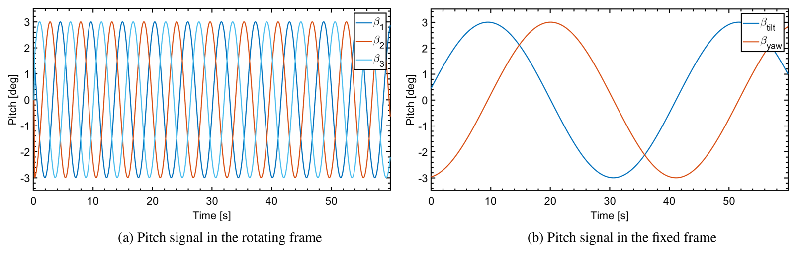
Figure 1 Pitch control signals used to generate a counterclockwise helix. The left figure shows the signal in the rotating frame, while the right figure shows the transformed signal in the fixed frame by using the MBC transform.

In practice, the helix approach is implemented by applying sinusoidal signals to the tilt (β_tilt) and yaw (β_yaw) angles. The frequency at which these signals are varied is characterized by the non-dimensional Strouhal number St:

$$\begin{array}{}\text{(3)}& \mathrm{St}={\displaystyle \frac{f_{\mathrm{e}}D}{U_{\mathrm{\infty }}}}\text{,}\end{array}$$

where f_e is the excitation frequency of the tilt and yaw commands, D is the rotor diameter, and U_∞ is the free stream wind velocity. Strouhal values are generally selected between 0.2 and 0.4, as recommended by previous work (Frederik et al., 2020b, a). This leads to the tilt and yaw pitch commands for helix wake mixing as shown by the following equation:

$$\begin{array}{}\text{(4)}& \left[\begin{array}{c}{\mathit{\beta }}_{\mathrm{tilt}}\\ {\mathit{\beta }}_{\mathrm{yaw}}\end{array}\right]=\left[\begin{array}{c}A\sin \left({\mathit{\omega }}_{\mathrm{e}}t\right)\\ A\sin ({\mathit{\omega }}_{\mathrm{e}}t\pm \mathit{\pi }/\mathrm{2})\end{array}\right]\text{,}\end{array}$$

where A is the amplitude of helix excitation, usually no larger than a few degrees due to practical constraints such as pitch rate limitations (Taschner et al., 2023), and ω_e=f_e2π.

Two helix variants are distinguished by a phase difference of $+\mathit{\pi }/\mathrm{2}$ and $-\mathit{\pi }/\mathrm{2}$ between the tilt and yaw pitch signals, resulting in a clockwise (CW) and counterclockwise (CCW) helix, respectively. While the actuation frequency in the fixed frame remains identical for both variants, the actual frequency applied by the pitch actuator varies once the tilt and yaw control commands are mapped to the rotating frame. This mapping leads to a helix frequency in the rotating frame of ω_r±ω_e (1P±f_e), depending on whether the helix is CW or CCW. Generally, a CCW helix results in higher farm-level energy gains (Taschner et al., 2023), while the CW helix is favored for lower damage to the pitch bearing (van Vondelen et al., 2023), which can be explained by the lower effective actuation frequency of 1P−f_e. In this work, the CCW helix is selected due to better energy gain.

2.2 Simulation tools

This study employs the NREL 5 MW wind turbine as the object of study; see Jonkman et al. (2009) for details. This turbine is widely used in wind energy research, offering a well-established benchmark. All simulations are conducted using QBlade (Marten et al., 2013), which uses a free-wake vortex method to simulate the flow field and the wake around the turbine. This method is known for its accuracy in the near wake and for being computationally more efficient than the LES method (Shaler et al., 2020). Although free-wake vortex methods may suffer from numerical instabilities in the far wake (van den Berg et al., 2023), this limitation is not critical for this study, as the downstream turbine is positioned within the near- to mid-wake region. This placement is sufficient to capture relevant wake dynamics, as demonstrated in Marten et al. (2020).

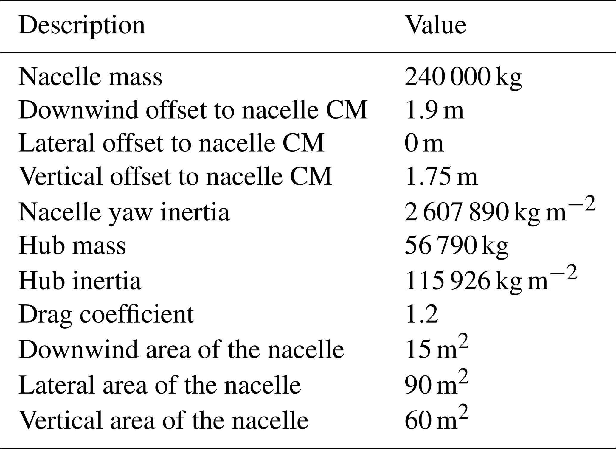
This work assumes that the dynamics of the hub vortex aft of the hub and nacelle are adequately resolved. However, this can be challenging in practice. In QBlade, the hub and nacelle properties of the NREL 5 MW wind turbine, including mass and inertia, are specified in Table 1. In QBlade, the nacelle is modeled with limited fidelity. While this is unlikely to influence the mean downwind velocity field in the far wake, it can influence the turbine power fluctuations and turbulence kinetic energy, as noted in the work of Foti et al. (2019). Moreover, Santoni et al. (2017) supports this experimentally. The study of Coquelet et al. (2024) further shows that the rotating pattern of the hub vortex still holds in the LES when the helix approach is applied. This suggests that the data-processing pipeline developed in this work, which is based on tracking the motion of the hub vortex, remains applicable despite these modeling limitations. Nevertheless, future work should validate the proposed control framework using a high-fidelity simulation environment where the aerodynamics of the nacelle are more accurately modeled, enabling a more comprehensive assessment of the system's behavior.

Table 1 Parameters of the hub and nacelle in QBlade of the NREL 5 MW wind turbine. “CM” stands for “center of mass”.

Lastly, the QBlade setup for aerodynamic simulation in this work is chosen under the principle of finding a trade-off between computational time and accuracy. Both wake modeling and the vortex modeling settings influence this balance: the former directly regulates the number of elements in the wake, while the latter are settings that influence vortex performance. The simulation settings used in this work follow those in van den Berg et al. (2023), as the two-turbine configurations are identical.

3 Closed-loop active wake mixing framework

This section serves as the core contribution of this paper: the proposed structure and design of the closed-loop active wake mixing framework. The following section focuses on the overall framework structure, followed by the design details about the lidar and control subsystems. Note that some details of the design can be found in the Appendix section. The goal of this section is to provide a high-level overview.

3.1 Overall framework structure

To enable lidar-based closed-loop wake mixing control within a wind farm, two main tasks must be considered: (1) the measurement task and (2) the control task. Thus, the overall system is designed to have two subsystems, each dedicated to fulfilling one of these tasks:

1. The lidar subsystem consists of a lidar facing downwind and a supporting pipeline for data processing. The design should fulfill two functionalities in real time:

   • helical wake data sampling

   • helical wake feature acquisition.

2. The control subsystem consists of a controller and the supporting components for closed-loop control. The design should fulfill the functionality of the following:

   • generate individual blade pitch inputs β_i based on real-time flow measurements

   • correct the helical wake based on the current output of the system and the given reference, compensating for any detected misalignment.

Consequently, the block diagram of the overall system is constructed as shown in Fig. 2. The design of the overall framework structure is inspired by the work of Raach et al. (2017).

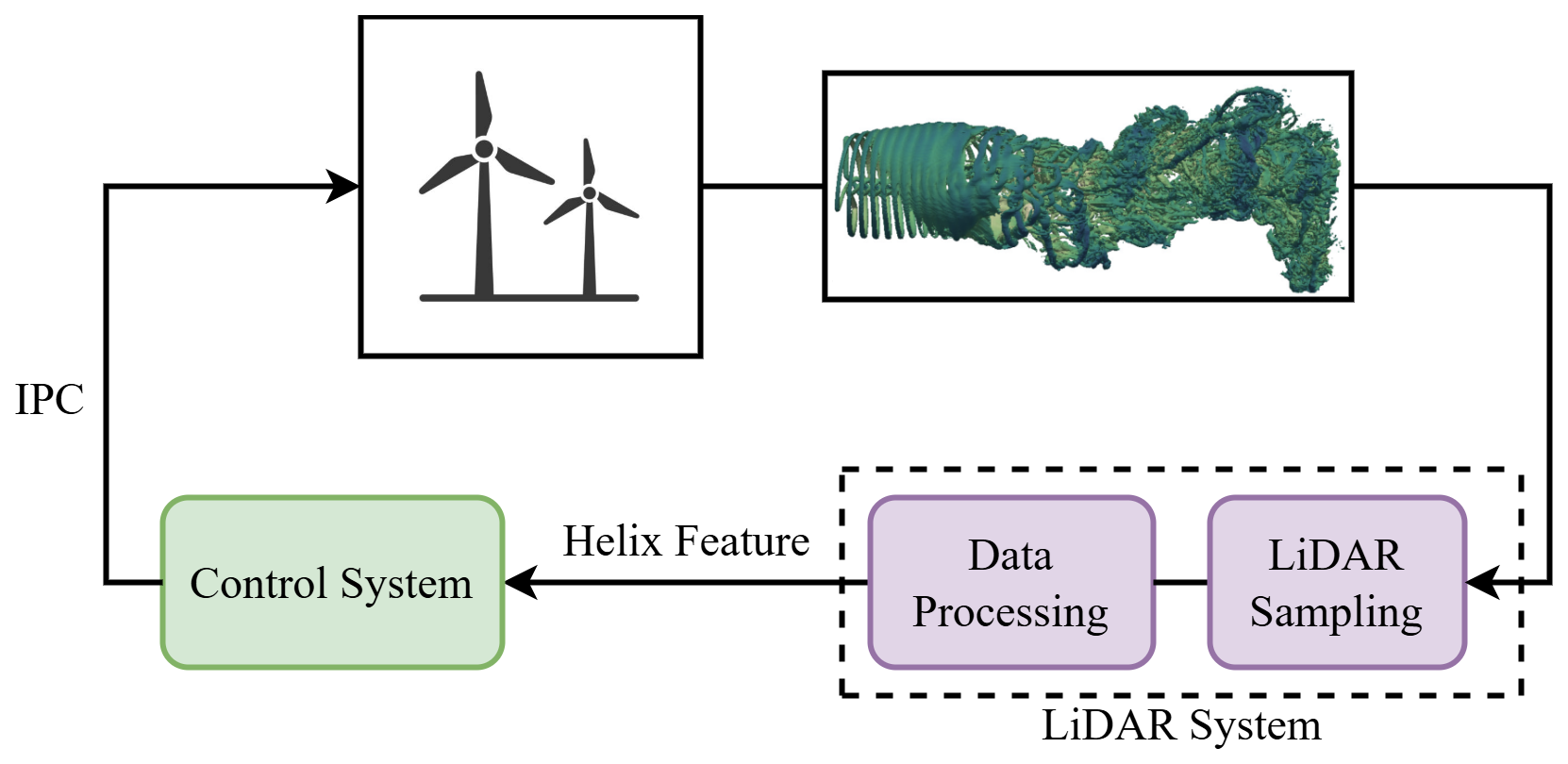
Figure 2 The diagram of the overall closed-loop control system consisting of the lidar subsystem and the control subsystem. The helical wake figure is adopted from the work of Korb et al. (2023).

3.2 Lidar subsystem design

To achieve the aforementioned functionalities, this section first presents the lidar configuration, supporting assumptions, and modeling approach. Subsequently, a feature for control is then selected. Finally, a coordinate transformation similar to the MBC transform is introduced to simplify the controller design.

3.2.1 Lidar setup and modeling

Lidar is a remote sensing method for measuring wind speed that has gained attention in the wind energy industry in recent years. It enables additional wake measurements to be incorporated into wind turbine controllers, thereby facilitating the development of advanced control strategies (Scholbrock et al., 2016). A detailed explanation of the lidar, the model, and the practical concerns can be found in Appendix A. In this work, we adopt a continuous-wave lidar due to its uniform return time of all measurements, which simplifies controller design.

Figure 3 shows a three-dimensional view of the lidar setup: a lidar is mounted on the top of the wind turbine nacelle, orienting downwind. The lidar measures the wind speed information of a plane with the same diameter as the rotor disk with a focal distance of 1D. This distance is chosen as a trade-off between wake data quality, measurement feasibility, and the upper bandwidth limit of the controller imposed by output delay, further discussed in Sect. 3.3. Furthermore, the lidar captures the flow information across the entire rotor disk by simultaneously sampling 80 points uniformly distributed in the Cartesian coordinate system. The number of sampling points is determined to balance the spatial resolution and the computational cost. Lastly, the lidar is modeled to have a sampling frequency of 10 Hz to ensure consistency with the QBlade simulation time step of 0.1 s.

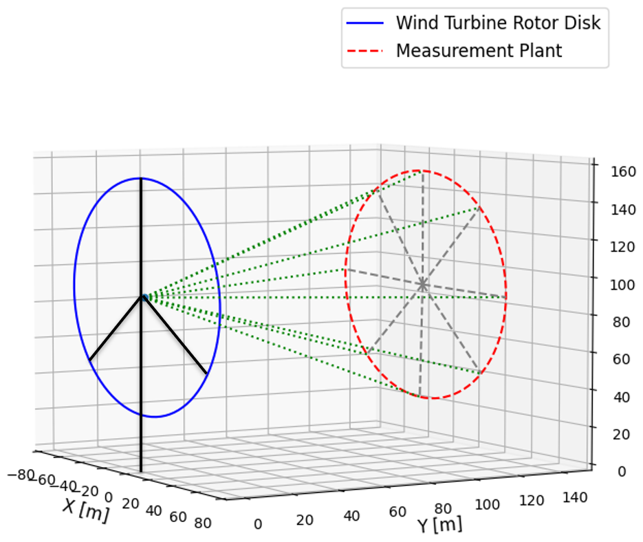
Figure 3 The three-dimensional view of the lidar setup.

3.2.2 Helix feature extraction

This section identifies a suitable controlled variable in the helical wake experimentally by analyzing the lidar-sampled data in simulations with the helix approach being activated.

Figure 4 Lidar sampling snapshots over a complete helix cycle T_e.

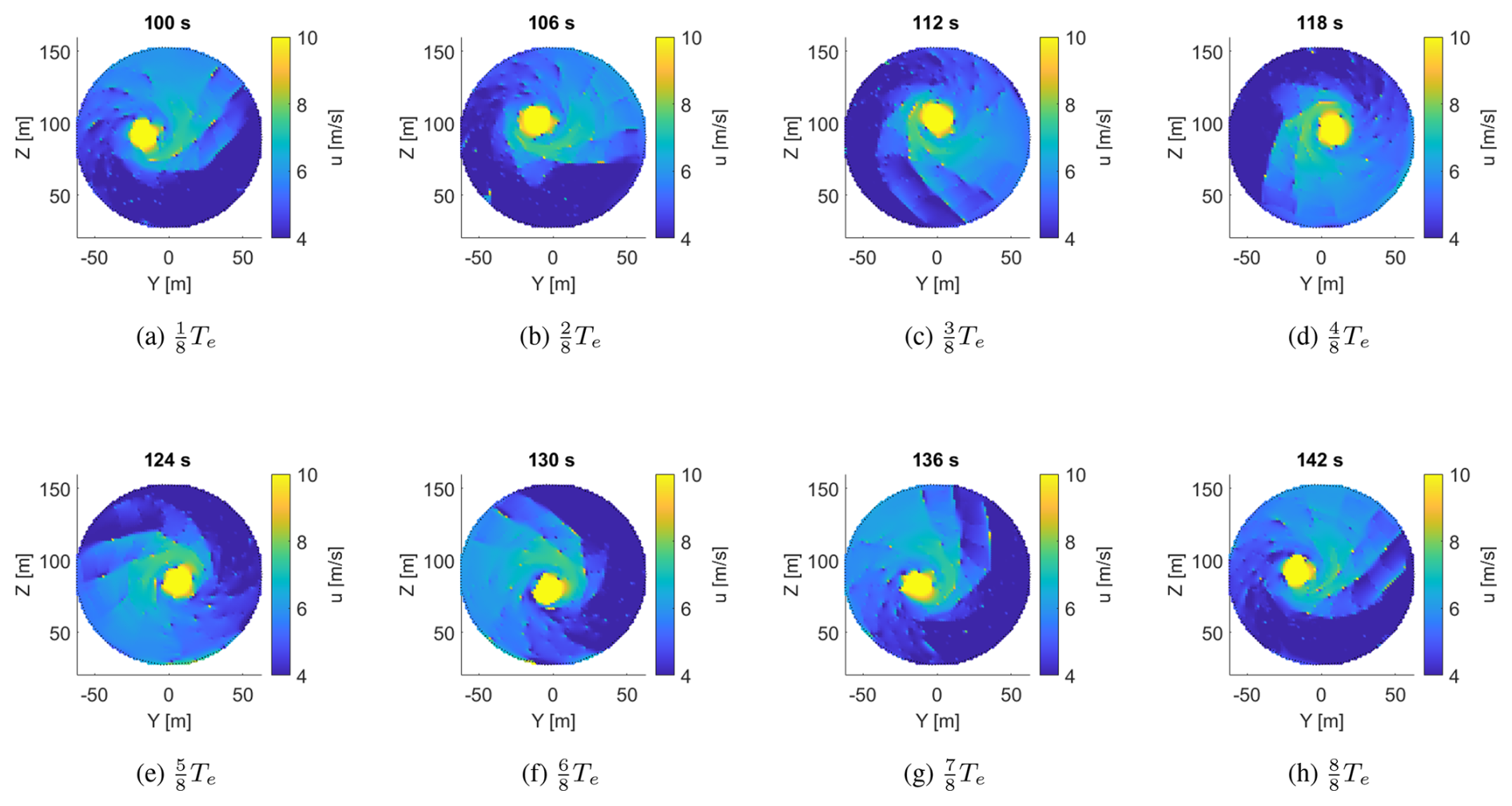
Figure 4 presents lidar sampling snapshots in QBlade over a complete helix cycle T_e. A counterclockwise (CCW) helix is applied with a Strouhal number of St=0.3, a uniform inflow wind speed of 10 m s⁻¹, and a helix amplitude of 3°. In the figure, wind speed is visualized through a color map, where higher velocities correspond to brighter shades. A distinct high-velocity region is observed rotating at the excitation frequency f_e, corresponding to the hub vortex of the wind turbine. This structure extends along the streamwise direction and has been previously documented in Iungo et al. (2013). The findings of Coquelet et al. (2023) further confirm the existence and rotational behavior of the hub vortex in helical wakes. Additionally, we analyzed sampled data under varying wind conditions, including vertical shear (exponential factor 0.2), turbulence (intensity 6 %), and their combination, while maintaining an average wind speed of 10 m s⁻¹. In all cases, the hub vortex remains distinguishable and retains its rotational behavior.

Experiments were conducted by randomly varying the helix amplitude between 1 and 6° and the Strouhal number between 0.1 and 0.4 while recording the rotation magnitude and frequency of the hub vortex. These parameter ranges were selected as the regime in which the helix is most effective; see Taschner et al. (2023). The correlation between the hub vortex rotation magnitude and the helix amplitude was found to be 0.9987, and the correlation between the hub vortex rotation frequency and the Strouhal number was 0.9995. These results show that helix amplitude changes directly affect hub vortex rotation magnitude, while Strouhal number changes affect rotation frequency. This strong correlation indicates that controlling the hub vortex is equivalent to controlling the helical wake. Additionally, the hub vortex is readily distinguishable through signal filtering due to its elevated velocity. It is therefore selected as the controlled variable of the helical wake.

3.2.3 Helix frame transformation

A noticeable characteristic of the hub vortex is its continuous rotation relative to the fixed frame at the helix frequency f_e. To simplify the controller design, the helix frame transformation proposed by van Vondelen et al. (2025b) is employed to map the hub vortex from the fixed frame to the helix frame, in which the vortex appears relatively stationary.

Table 2 The frequency of helical wake in different coordinate frames.

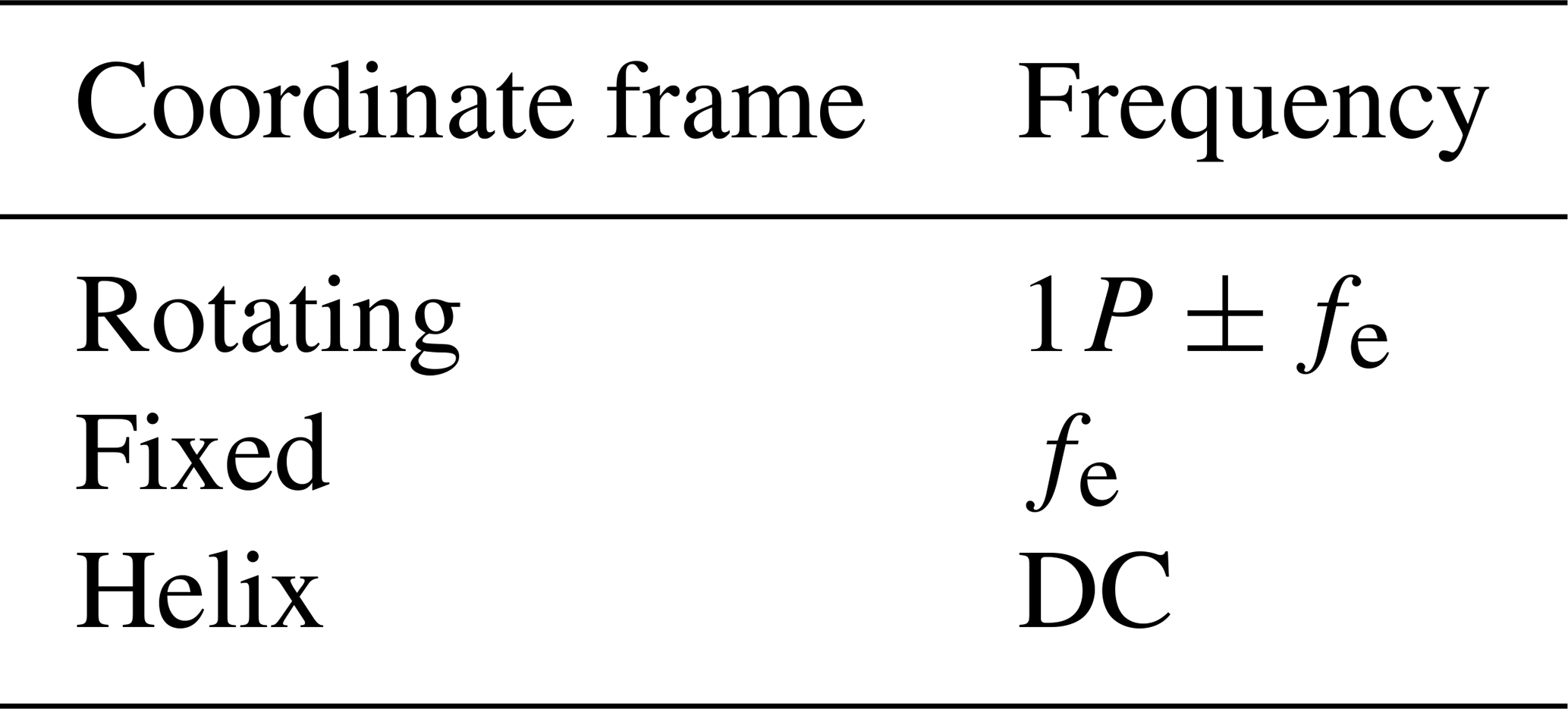
To achieve this, the principle of modulation–demodulation is applied, transforming the rotating helix from the rotating coordinate frame to the helix coordinate frame, shifting the 1P+f_e helix rotation (assuming a CCW helix) to the DC gain. The summary of the frequency of the helix in different coordinate frames is shown in Table 2. The derivation of the helix frame transform resembles the MBC transform. The main difference is that the excitation frequency ω_e is included:

$$\begin{array}{}\text{(5)}& \left[\begin{array}{c}{\mathit{\beta }}_{\mathrm{col}}^e\\ {\mathit{\beta }}_{\mathrm{tilt}}^e\\ {\mathit{\beta }}_{\mathrm{yaw}}^e\end{array}\right]=T_{\mathrm{cm}}\left({\mathit{\omega }}_{\mathrm{e}}t\right)\left[\begin{array}{c}{\mathit{\beta }}_{\mathrm{1}}\\ {\mathit{\beta }}_{\mathrm{2}}\\ {\mathit{\beta }}_{\mathrm{3}}\end{array}\right]\text{,}\end{array}$$

where

$$\begin{array}{}\text{(6)}& T_{\mathrm{cm}}\left({\mathit{\omega }}_{\mathrm{e}}t\right)={\displaystyle \frac{\mathrm{2}}{\mathrm{3}}}\left[\begin{array}{ccc}\mathrm{1}/\mathrm{2}& \mathrm{1}/\mathrm{2}& \mathrm{1}/\mathrm{2}\\ \cos \left({\mathit{\omega }}_{\mathrm{1}}\right)& \cos \left({\mathit{\omega }}_{\mathrm{2}}\right)& \cos \left({\mathit{\omega }}_{\mathrm{3}}\right)\\ \sin \left({\mathit{\omega }}_{\mathrm{1}}\right)& \sin \left({\mathit{\omega }}_{\mathrm{2}}\right)& \sin \left({\mathit{\omega }}_{\mathrm{3}}\right)\end{array}\right]\text{,}\end{array}$$

and ${\mathit{\omega }}_i={\mathit{\psi }}_i+{\mathit{\omega }}_{\mathrm{e}}t$, representing the CCW helix frequency. A detailed explanation of the helix frame transform can be found in Appendix B. As a result, this transform maps the rotating input and output signals, (β_tilt,β_yaw) and (z,y), to a more static signal representation, (${\mathit{\beta }}_{\mathrm{tilt}}^e,{\mathit{\beta }}_{\mathrm{yaw}}^e$) and (z^e,y^e), simplifying the subsequent controller design. Note that mean centering needs to be applied to signals to eliminate extra oscillating components.

As a result, the overall lidar-processing pipeline is developed as shown by Fig. 5, consisting of three parts:

1. Lidar sampling. Capture wind speed data u_LOS at the specified focal distance of 1D downwind.

2. Data processing.

   • Hub vortex filter. Extract the coordinates of the hub vortex in the rotating frame, (y,z), by isolating the high-speed region and averaging the positions of the filtered points.

   • Low-pass filter. Remove high-frequency noise from the signal. The finite-impulse response (FIR) filter is chosen for its desirable properties like guaranteed stability, absence of limit cycles, and linear phase (Neuvo et al., 1984). The filter order is selected as 50 in the trade-off between phase delay and filtering performance, and the cut-off frequency of the low-pass filter is chosen as 0.05 Hz since the helix is in the frequency of 0.0238 Hz.

3. Helix frame transform. Map the hub vortex from the fixed frame to the helix frame where it becomes static.

Figure 5 Flow chart of the lidar data-processing pipeline.

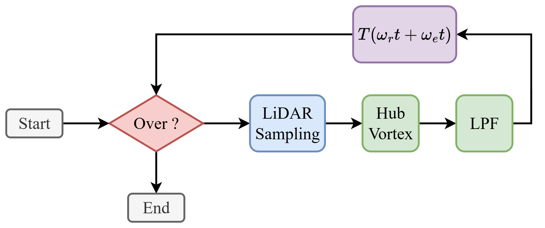
Figure 6 presents the output of the data-processing pipeline. The helix approach, configured with St=0.3 and $u=\mathrm{10}\mathrm{m}{\mathrm{s}}^{-\mathrm{1}}$, is activated during two discrete intervals: from 50 to 150 s and from 250 to 350 s. Outside these periods, the wind turbine operates under baseline conditions. The result confirms that the pipeline effectively maps the rotating signals from the fixed frame to the helix frame. Although the signal in the helix frame is not fully static, likely due to residual noise that the low-pass filter cannot fully eliminate, a clear trend toward a constant value is still observable.

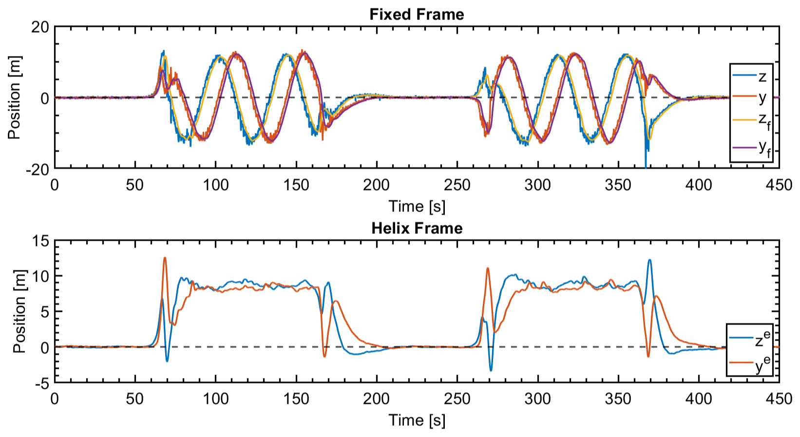
Figure 6 Output of the data-processing pipeline. The top panel shows hub vortex signals in the fixed frame; the bottom panel shows them in the helix frame. Here, (y,z) are the original signals, (y_f,z_f) the filtered ones, and (y^e,z^e) the results after applying the helix frame transform.

3.3 Control subsystem design

The main challenge of designing the control system is the presence of a time delay τ, as the wake needs to take time to travel to the measurement location. This delay τ is categorized as the output delay, defined as the delay between the time the system state or output changes and the time this change is observed (Zhang and Xie, 2007). For control purposes, two assumptions are made for the delay τ in this work:

1. The value of τ is assumed to align with Taylor's frozen turbulence hypothesis (Taylor, 1938) as introduced by Scholbrock et al. (2016), which states that the value of delay is only determined by the measurement distance x and the average inflow wind speed u_in:

   $$\begin{array}{}\text{(7)}& \mathit{\tau }=\mathit{\alpha }\cdot {\displaystyle \frac{x}{u_{\mathrm{in}}}}\text{.}\end{array}$$

   The coefficient α is used for calibrating the value.

2. The delay for each output y_i to each input u_j remains the same, since the helix frame transform does not alter the physical advection time of the yaw and tilt components of the helical wake, which reach the measurement point simultaneously. As a result, the dynamic of the system in the helix frame can be expressed as

   $$\begin{array}{}\text{(8)}& \left[\begin{array}{c}{z}^e\\ y^e\end{array}\right]=\underset{\mathbf{\text{G}}}{\underbrace{\left[\begin{array}{cc}{G}_{\mathrm{11}}\left(z\right)& G_{\mathrm{12}}\left(z\right)\\ G_{\mathrm{21}}\left(z\right)& G_{\mathrm{22}}\left(z\right)\end{array}\right]z^{-\mathit{\tau }}}}\left[\begin{array}{c}{\mathit{\beta }}_{\mathrm{tilt}}^e\\ {\mathit{\beta }}_{\mathrm{yaw}}^e\end{array}\right]\text{.}\end{array}$$

In this work, the average inflow wind speed of every case is set to be 10 m s⁻¹. Accordingly, a consistent delay time is found as T=11.2 s via Padé approximation.

Figure 7 The block diagram of the control system.

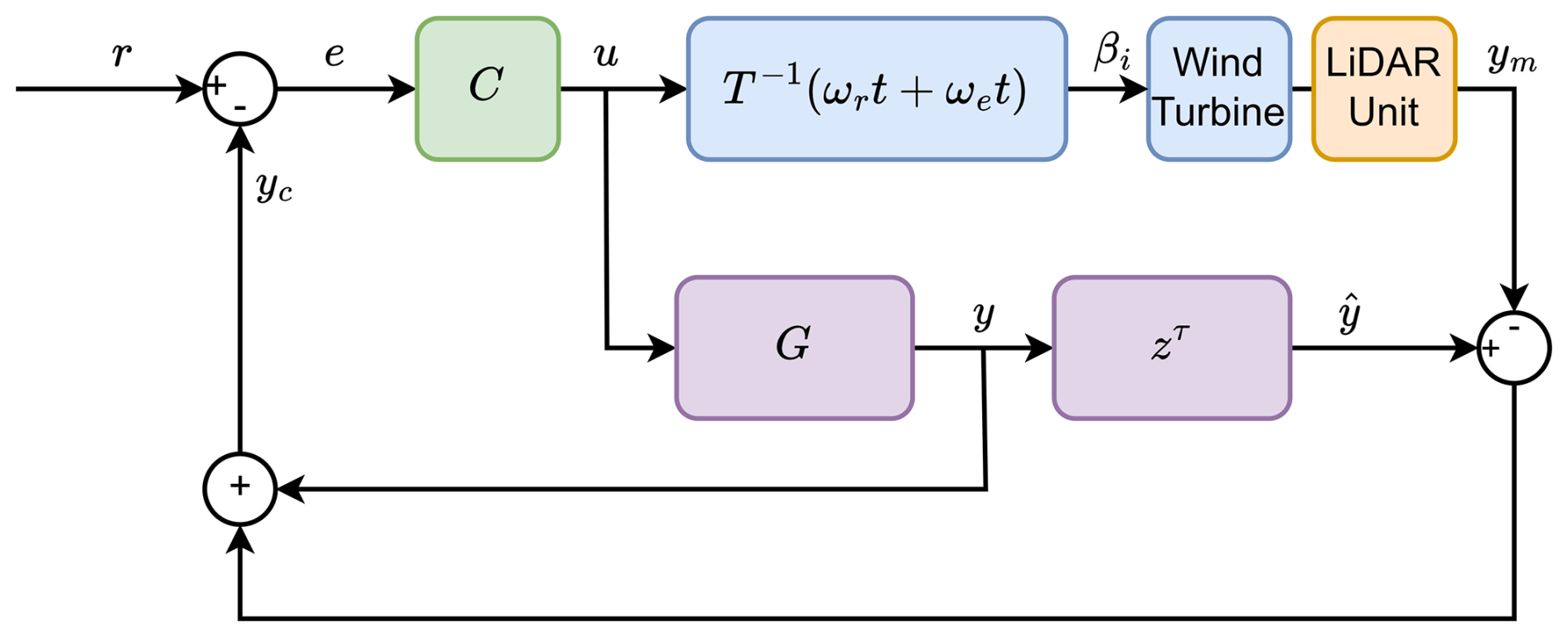
To control a delayed system, the Smith predictor based on internal model control (IMC) is adopted, as it effectively compensates for time-invariant delays. This approach is well-suited for systems with known constant dead time, as demonstrated in Abe and Yamanaka (2003). Figure 7 shows the general concept of the controller. The reference signal r is the desired coordinate of the hub vortex in the helix frame, represented by $[z_r^e,y_r^e{]}^T$. The control input u denotes the tilt and yaw pitch signal in the helix frame, expressed as $[{\mathit{\beta }}_{\mathrm{tilt}}^e,{\mathit{\beta }}_{\mathrm{yaw}}^e{]}^T$. Since the wind turbine cannot directly receive tilt and yaw signals, the inverse helix frame transformation $T^{-\mathrm{1}}({\mathit{\omega }}_{r}t+{\mathit{\omega }}_{\mathrm{e}}t)$ is applied to convert the inputs into the blade pitch signals β_i. Moreover, the lidar unit samples the wind turbine output and converts the hub vortex into the helix frame.

3.3.1 Internal model identification

The presented controller follows the idea of internal model control, in which the difference between the actual system output and a predicted output is used within the controller to regulate the system (Raach et al., 2017). Therefore, a model G that describes the dynamics of the helical wake effect, or the dynamics of $({\mathit{\beta }}_{\mathrm{tilt}}^e,{\mathit{\beta }}_{\mathrm{yaw}}^e)\to (z^e,y^e)$, is essential. In this work, the internal model G is acquired through system identification of the experimental data, focusing on wind speed $u_{\mathrm{in}}=\mathrm{10}\mathrm{m}{\mathrm{s}}^{-\mathrm{1}}$. The primary motivation for deriving this model is to simplify the subsequent controller design and to ensure computational efficiency. Since the proposed framework is intended for real-time implementation, the surrogate model must maintain a low computational cost. Since both input and output signals are mapped to the helix frame, where they exhibit approximately linear behavior, building a linear model is an effective choice.

The detailed introduction of the system identification process can be found in Appendix C. Consequently, the frequency domain response of the identified model is illustrated in Fig. 8, indicating several observations:

1. The identified system successfully captures the system dynamics within the frequency range.

2. The difference in steady-state magnitude between the diagonal and off-diagonal transfer functions indicates a degree of decoupling within the system. Specifically, the steady-state gains of G₁₁ and G₂₂ are positive, while those of G₁₂ and G₂₁ are negative. This implies that ${\mathit{\beta }}_{\mathrm{tilt}}^e$ influences z^e and ${\mathit{\beta }}_{\mathrm{yaw}}^e$ influences y^e predominantly in steady-state frequencies. The steady-state RGA matrix of $\left[\begin{array}{cc}\mathrm{0.9935}& \mathrm{0.0065}\\ \mathrm{0.0065}& \mathrm{0.9935}\end{array}\right]$ supports this further.

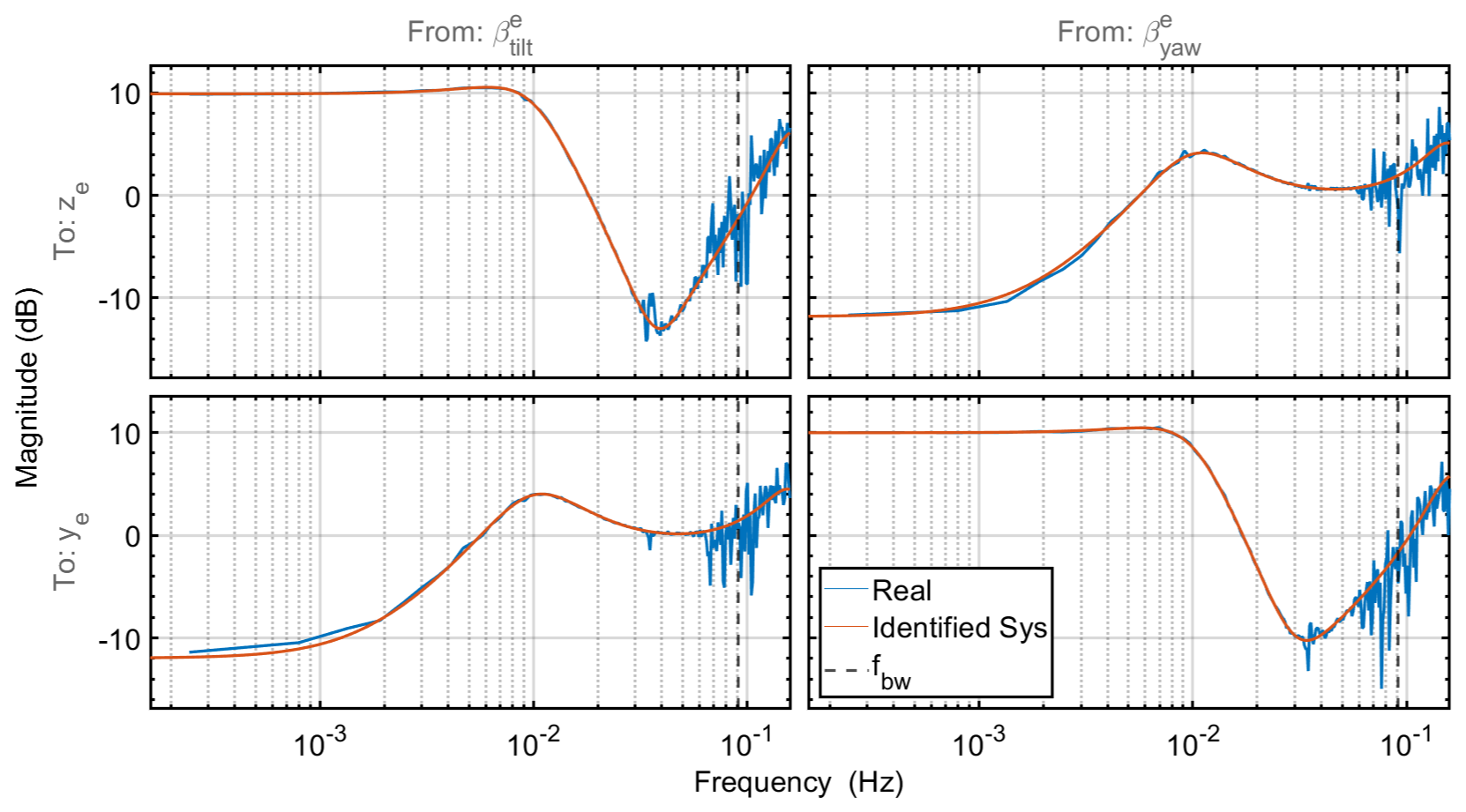
Figure 8 Comparison of the PBSID-opt identified model (orange) against the spectral averaged input and output data (blue). The dashed line indicates the estimated bandwidth frequency, which defines the frequency of interest.

Since this research employs a linear system identification method, G is linearly time invariant. Consequently, G is only applicable within a specific operating range. Although the model G exhibits steady-state decoupling, strong couplings at the bandwidth frequency, supported by the RGA matrix at the bandwidth frequency of $\left[\begin{array}{cc}-\mathrm{1.2780}& \mathrm{2.2780}\\ \mathrm{2.2780}& -\mathrm{1.2780}\end{array}\right]$, complicate the design of a decentralized controller combined with a pre-compensator, such as a diagonal control structure adopted in van Vondelen et al. (2025b). A diagonal controller could be implemented by choosing a very low crossover frequency, but the slow reaction time would offer limited benefit. Consequently, an ℋ_∞ controller is adopted for its robustness to uncertainty and modeling errors in MIMO systems.

3.3.2 ℋ_∞ controller synthesis

The ℋ_∞ controller synthesis uses the general control configuration, as shown in Fig. 9, where P is the generalized plant and K the generalized controller.

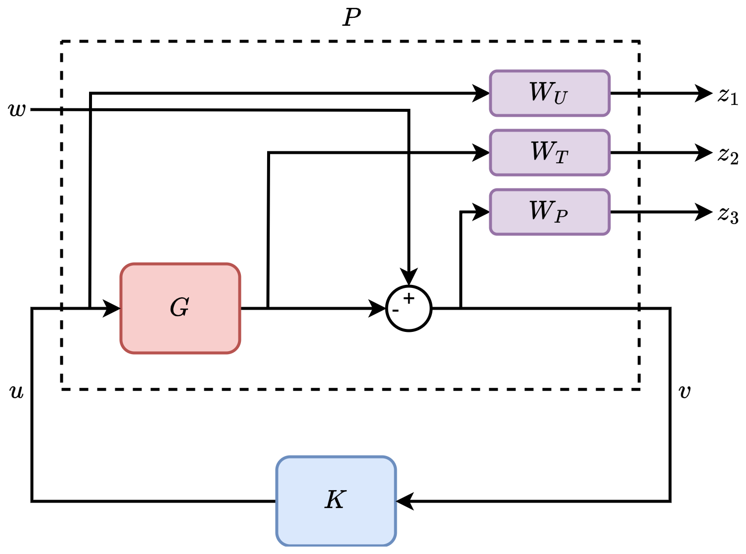
Figure 9 Generalized plant P with performance signals z₁, z₂, and z₃ and input w. Furthermore, G denotes the identified model; K represents the controller; and W_P, W_U, and W_T represent the performance weights.

The idea of formulating a general control problem is to find a controller K to minimize the ℋ_∞ norm of the transfer function from input w to performance output z; see Skogestad and Postlethwaite (2005). Weight functions W_U, W_T, and W_P are integrated to provide different weighted performance measures from outputs z₁ to z₃. The ℋ_∞ controller synthesis considers three criteria to design and evaluate the performance of the controller: the sensitivity S, the complementary sensitivity T, and the controller sensitivity U, defined as

$$\begin{array}{}\text{(9)}& S={\displaystyle \frac{\mathrm{1}}{\mathrm{1}+GK}}\text{,}T={\displaystyle \frac{GK}{\mathrm{1}+GK}}\text{,}U={\displaystyle \frac{K}{\mathrm{1}+GK}}\text{.}\end{array}$$

For the physical interpretation, S gives the transfer function from the disturbance to the system output, T is the transfer function from the reference to the output, and −U is the transfer function from the disturbance to the control signal.

As a result, the controller K is obtained by solving the mixed-sensitivity optimization problem, as defined in Eq. (10):

$$\begin{array}{}\text{(10)}& \underset{K}{min}{∥\begin{array}{c}{W}_{P}S\\ W_{T}T\\ W_{U}U\end{array}∥}_{\mathrm{\infty }}=\underset{K}{min}{∥\begin{array}{c}{W}_P(\mathrm{1}+GK{)}^{-\mathrm{1}}\\ W_{T}GK(\mathrm{1}+GK{)}^{-\mathrm{1}}\\ W_{U}K(\mathrm{1}+GK{)}^{-\mathrm{1}}\end{array}∥}_{\mathrm{\infty }}\text{.}\end{array}$$

For the closed-loop system, a good disturbance rejection is desired, and therefore, S should be small for low frequencies. Furthermore, the control effort should be limited by having a roll-off in T after the bandwidth. Based on this, the weight functions are designed. W_P(s) is designed as a low-pass filter with the form of

$$\begin{array}{}\text{(11)}& W_P\left(s\right)={\displaystyle \frac{s/M+{\mathit{\omega }}_{\mathrm{cl}}}{s+A{\mathit{\omega }}_{\mathrm{cl}}}}\text{,}\end{array}$$

where ω_cl denotes the desired closed-loop bandwidth, A is the desired disturbance attenuation inside the bandwidth, and M is the desired bound on $\left|\right|S|{|}_{\mathrm{\infty }}$ and $\left|\right|T|{|}_{\mathrm{\infty }}$. The upper bound M and lower bound A of S are set to M=10 and A=0.625, respectively. The desired closed-loop bandwidth ω_cl is set to ${\mathit{\omega }}_{\mathrm{cl}}=\mathrm{0.02}\mathrm{rad}{\mathrm{s}}^{-\mathrm{1}}$ due to the limitation introduced by the non-minimum-phase zeros of G(s). Specifically, the upper bound of ω_cl is selected to remain below $z/\mathrm{2}$, where z is the real part of the non-minimum-phase zeros in continuous time, as proven in Skogestad and Postlethwaite (2005). These non-minimum-phase zeros are likely introduced by unmodeled delays in the system: the residual pitch actuator delay that is not fully compensated for by the azimuth offset ψ_off, as well as the inherent downwind sensing delay. It remains unclear whether the intrinsic dynamics of the helical wake also contribute to this non-minimum-phase behavior. Therefore, future work should investigate whether the helix-induced dynamics influence the emergence of non-minimum-phase zeros.

The non-minimum-phase zero indirectly limits the controller gains for the stability requirement. Consequently, the controller weight function W_U(s) is designed as a band-limited high-pass filter to attenuate the control input in the high frequency as shown below:

$$\begin{array}{}\text{(12)}& W_U\left(s\right)=\mathrm{0.4}{B}^{\mathrm{2}}\cdot {\displaystyle \frac{s^{\mathrm{2}}+\sqrt{\mathrm{2}}{\mathit{\omega }}_{\mathrm{c}}+{\mathit{\omega }}_{\mathrm{c}}^{\mathrm{2}}}{s^{\mathrm{2}}+B\sqrt{\mathrm{2}}{\mathit{\omega }}_{\mathrm{c}}s+(B{\mathit{\omega }}_{\mathrm{c}}{)}^{\mathrm{2}}}}\text{.}\end{array}$$

Parameter B scales the frequency at which control effort starts to be limited, and ω_c is related to the cutoff frequency. In this study, B is selected as 10, and the crossover frequency ω_c is set to 0.15 rad s⁻¹ according to the pitch controller changing rate; a scaling factor of 0.4 is adopted to ensure the controller achieves the trade-off between performance and robustness without overly penalizing control effort. Finally, W_T(z) is kept at 0 since we focused on tracking performance and disturbance rejection at low frequencies (Skogestad and Postlethwaite, 2005).

4 Results and analysis

This section presents the results of the proposed control framework, including an evaluation of its reference tracking performance and its impact on power production and blade damage-equivalent loads (DELs) in both flapwise and edgewise directions.

4.1 Simulation setup

The proposed framework is evaluated in QBlade. The controller is tested by comparing it with the open-loop controller in four different wind conditions: uniform wind, shear, turbulence, and combined shear and turbulence.

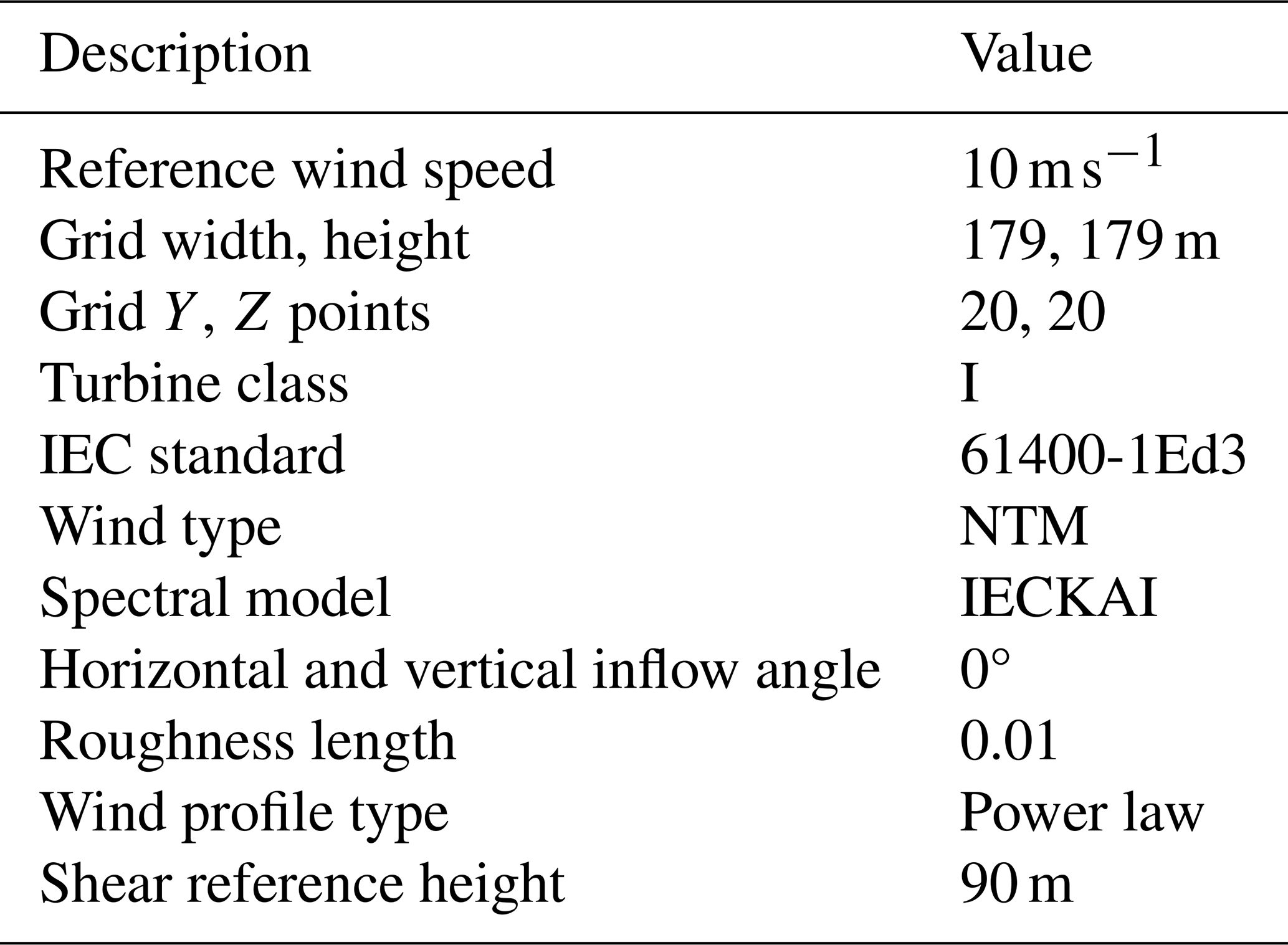
A two-turbine wind farm is created for simulation, where the downstream turbine is placed 4 rotor diameters (4D) away from the upstream turbine. This distance balances the trade-off between the QBlade simulation quality with realistic turbine spacing. The exponential factor of shear is set to 0.2, and the turbulence intensity (TI) is set to 6 % according to the IEC 61400-1 design standard to mimic the usual condition offshore (Burton et al., 2011). In this work, shear and turbulence are added by using the Turbulence Simulator (TurbSim); see Jonkman (2014). The primary parameters of the generated wind field are summarized in Table 3.

Table 3 Parameters of wind field generated by TurbSim.

The NREL 5 MW turbine is selected as the object of study. Its power-production operation is governed by two independent control systems: a generator-torque controller and a collective blade-pitch controller, designed to operate in the below-rated and above-rated wind speed range, respectively (Jonkman et al., 2009). The goal of the former is to maximize power capture below the rated wind speed, whereas the latter aims to regulate generator speed above the rated wind speed. In reality, the helix approach is typically implemented under below-rated wind conditions, where power losses are more substantial compared to those encountered in above-rated conditions (Frederik and van Wingerden, 2022). Consequently, a kω² torque controller is employed to maintain an optimal tip speed ratio to maximize the power production. The gain constant k is set to 2.3323 based on Jonkman et al. (2009).

To study the effect of the proposed control framework on power production and fatigue, eight cases are performed as listed in Table 4. Each scenario was evaluated via a single simulation run, serving as a proof of concept to demonstrate the efficacy of the proposed control framework. For all cases, the average inflow wind speed is kept constant at $u_{\mathrm{in}}=\mathrm{10}\mathrm{m}{\mathrm{s}}^{-\mathrm{1}}$, and the Strouhal number is set to St=0.3. All helical wakes generated rotate in the CCW direction. Each simulation ran for 15 min, with the initial 300 s excluded from analysis to account for wake development and transient effects.

The main goal of this study is to eliminate variations in the helical wake introduced by external wind conditions, generating a more consistent helical wake relative to the uniform-wind case. In our simulation, we found that the performance of the wind farm varies under different wind conditions, accompanied by changes in helical wake structure. Thus, we aim to ensure this consistency by eliminating the variation in the helical wake. As a result, the output of OL₁ in the helix frame is used as the reference for all cases. This simple target was selected to demonstrate the feasibility of the closed-loop helix approach as a proof of concept. However, this assumption does not guarantee the optimality of the decision. Additionally, it is crucial to acknowledge the difficulty of defining a definitive reference point as priorities vary across different interests, and thus the given reference varies. For instance, as shown in a later section, both the upstream and the downstream turbines have significantly increased load under shear despite increases in power. Thus, eliminating variations in the wake might not be a good idea in this case; instead, a reference that balances the power production increase and the fatigue load increase could be given. Furthermore, in the case of extreme wind conditions like high veer, the chosen reference may simply be infeasible. Therefore, the reference signal should be selected flexibly depending on the operator, and future studies should explore whether a consistent helical wake matches the stakeholders' interest and explore more condition-based reference choices.

Table 4 Overview of all test cases. “WT₁” and “WT₂” stand for upstream and downstream turbines. In the wind column, the shear exponential factor and turbulence intensity are listed. Moreover, “CCW” stands for counterclockwise, and “Greedy” means only the basic kω² torque controller was implemented.

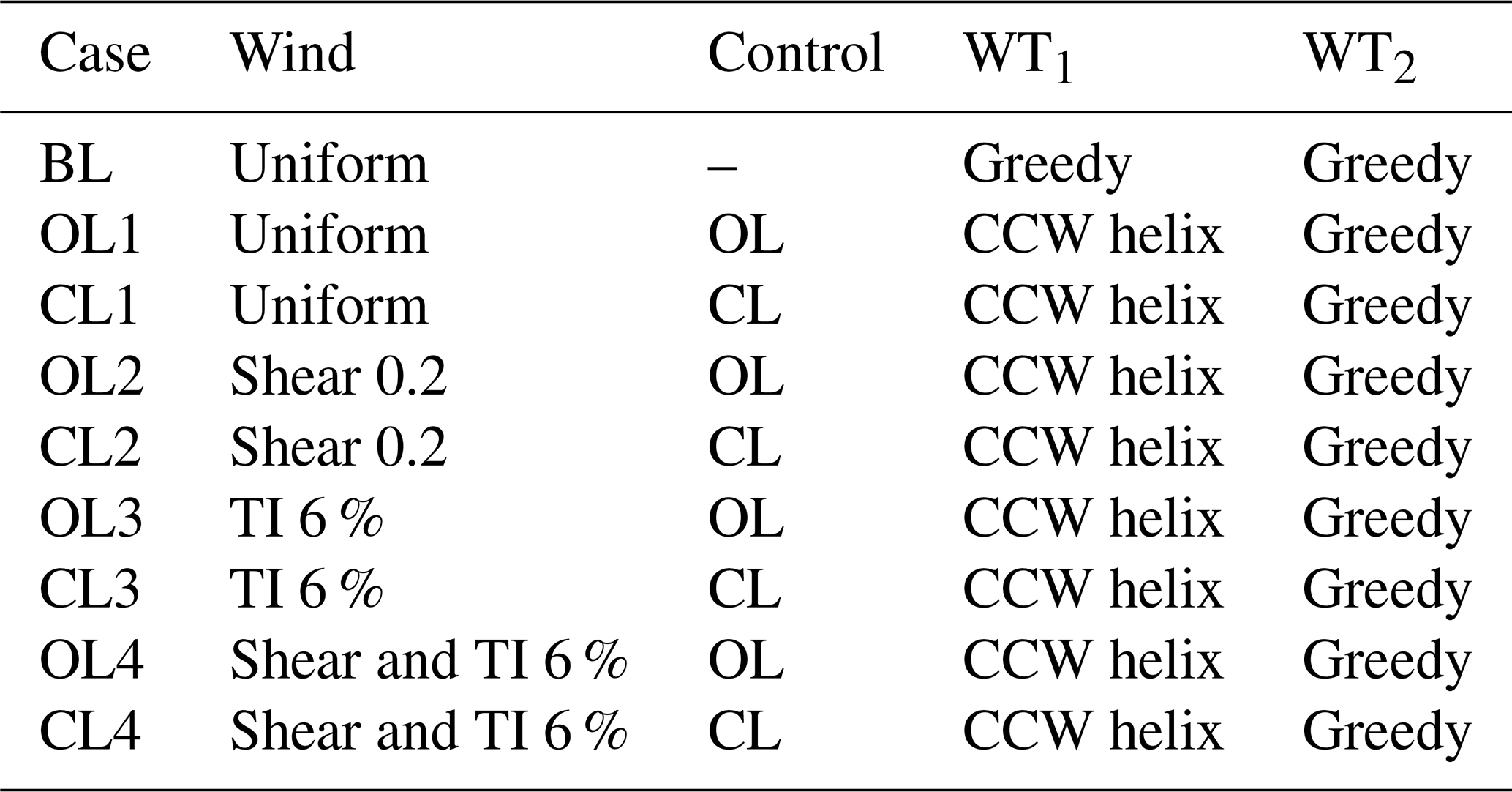
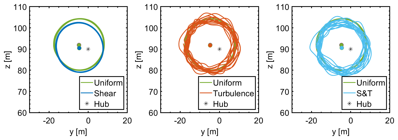
Figure 10 Comparison of hub vortex trajectory in the fixed frame of open-loop cases in uniform-wind conditions (OL₁) to shear (OL₂), turbulence (OL₃), and combined shear and turbulence (OL₄). “Hub” denotes the hub of the wind turbine.

4.2 Open-loop helix in different wind conditions

Figure 10 illustrates the hub vortex trajectory in the fixed frame of different wind conditions compared to the uniform-wind case. The figure reveals a consistent bias in the z direction under shear conditions, increased oscillations with turbulence, and the presence of both bias and oscillation when shear and turbulence are combined. These trajectory changes impact both power production and fatigue loading, as shown in Fig. 11. The results reveal the following:

1. Shear. When only shear is present, the power loss of both turbines is evident. This is consistent with the findings of Parinam et al. (2023), which report that a higher shear resulted in a reduction in wake recovery and a lower TI in the wake as a whole, thereby increasing the power loss of turbines located downstream. Moreover, the cumulative blade edgewise and flapwise DEL decreased.

2. Turbulence. Compared to the helix in the uniform-wind case, OL₃ shows increments in power production and fatigue for both turbines. This can be explained by the increased TI and the natural mixing effects of turbulence (van den Berg et al., 2023).

3. Combined shear and turbulence. When both shear and turbulence are present, the wind farm has a cumulative loss in power production and cumulative increments in both flapwise and edgewise DEL.

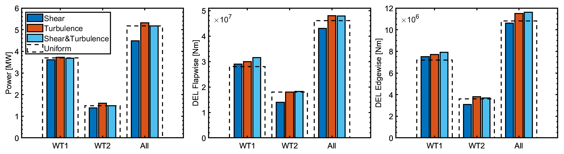
Figure 11 The power and DEL of OL₂ (blue), OL₃ (orange), and OL₄ (sky blue) compared to case OL₁ (dashed line). “WT1”, “WT2”, and “All” denote the upstream turbine, the downstream turbine, and the entire two-turbine wind farm.

The comparison offers insights into the expected behavior of the closed-loop controller. Given that the goal of this study is to generate a more consistent helix, the corresponding objectives of the controller in terms of the hub vortex trajectory can be summarized:

1. Uniform. The performance of CL₁ should match that of OL₁ by generating an identical helix.

2. Shear. Compared to OL₂, the controller should rectify the steady-state bias.

3. Turbulence. The controller is expected to mitigate the extra oscillation of the hub vortex introduced by the turbulence. However, because the dominant turbulence frequency exceeds the roll-off frequency of the controller, this mitigation effect is going to be compromised. Thus, complete stabilization of the hub vortex rotation is unlikely. Nevertheless, the controller will still attempt the mitigation by generating dynamic pitch inputs.

4. Combined shear and turbulence. The controller should correct the bias while trying to mitigate the oscillation as much as possible.

4.3 Closed-loop framework performance and analysis

This section shows the performance of the closed-loop system. In uniform-wind conditions, both the open-loop and the closed-loop systems generate identical helical wake structures, confirming the effectiveness of the proposed framework. For brevity, only cases where shear and turbulence are added are presented.

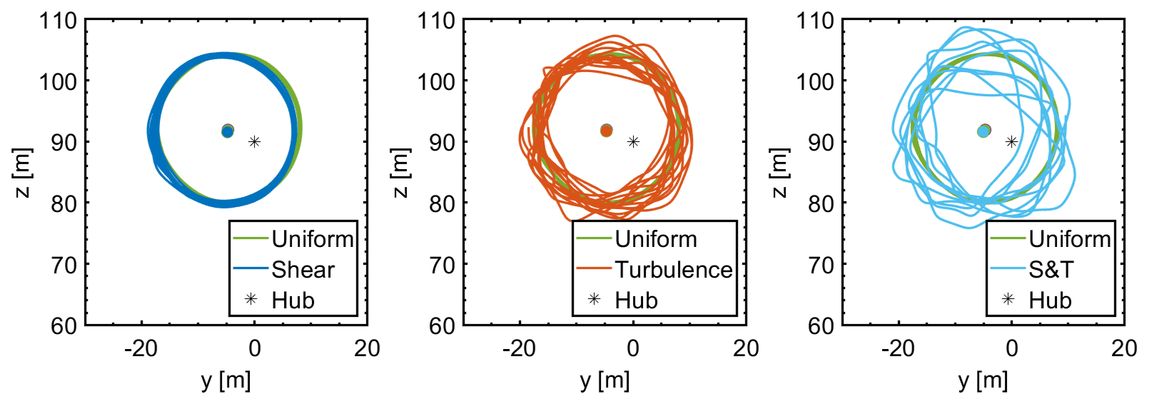
Figure 12 Comparison of hub vortex trajectory in the fixed frame of the uniform-wind open-loop case (OL₁) to closed-loop cases under shear (CL₂), turbulence (CL₃), and combined shear and turbulence (CL₄).

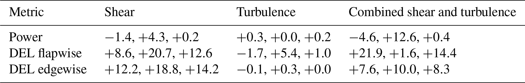
Figure 12 illustrates the hub vortex trajectory generated by the closed-loop system compared to the reference. The corresponding change in the wind farm performance compared to the open-loop system is shown in Table 5. The performance and the corresponding analysis of these three different wind conditions are presented in the following sections.

Table 5 Comparison of percentage change in performance between open-loop and closed-loop frameworks under three wind conditions. All values are presented as percentages (%). Each cell is formatted as WT₁,WT₂, and All, where WT₁, WT₂, and All stand for the upstream turbine, the downstream turbine, and the overall wind farm, respectively.

4.3.1 Shear

Under the shear condition, the closed-loop system effectively corrects the steady-state bias in the hub vortex trajectory, leading to a measurable increase in downstream power production. This improvement is driven by the redirection of the helical wake, which results in higher average inflow wind speeds at the 4D downstream position for the closed-loop case (CL₂) compared to the open-loop baseline (OL₂). However, these gains are accompanied by a trade-off between increased DELs for both turbines and a slight reduction in upstream power. These effects stem from the more aggressive control actions required for bias correction. Specifically, as shown in Fig. 13, the closed-loop controller superimposes oscillatory components onto the tilt and yaw pitch inputs (${\mathit{\beta }}_{\text{tilt}}^e$ and ${\mathit{\beta }}_{\text{yaw}}^e$). This contrasts with the constant inputs used in the OL₂ case and likely contributes to the increased fatigue observed in the upstream turbine.

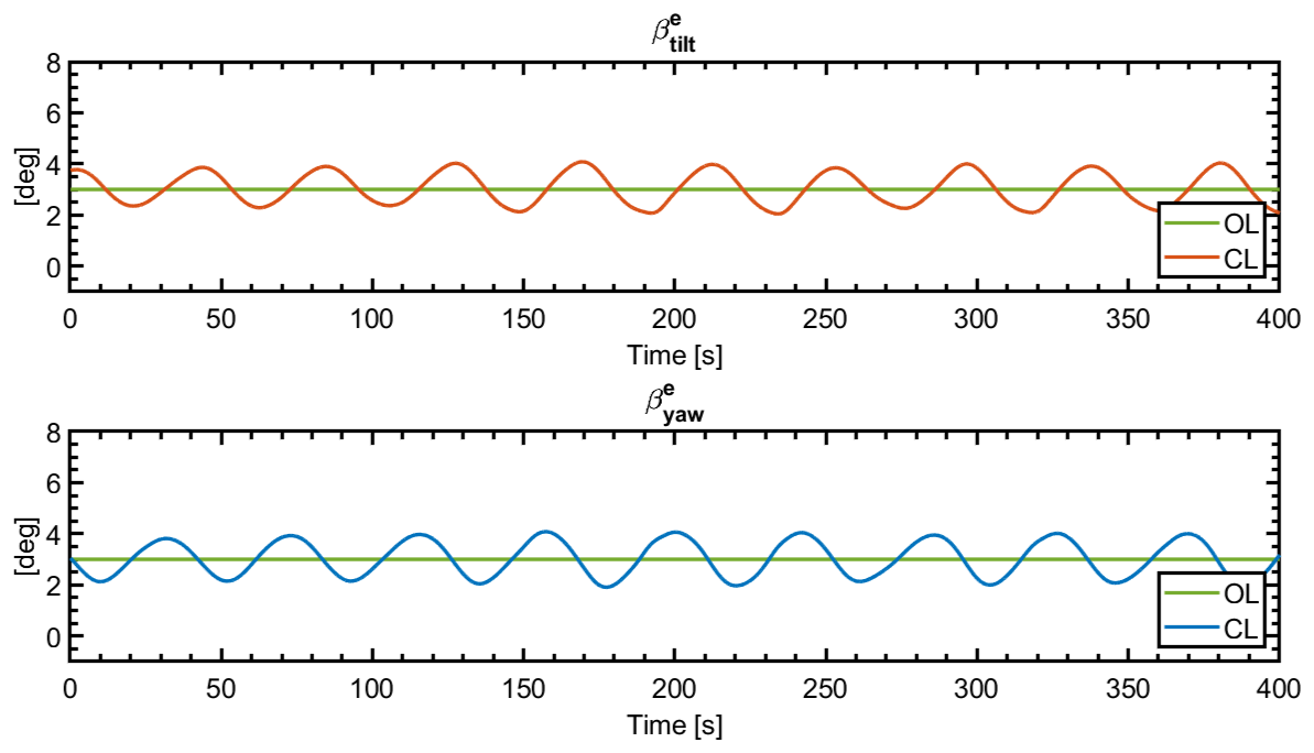
Figure 13 The comparison of pitch inputs in the helix frame between the open-loop (OL₂) and closed-loop (CL₂) case under shear. Compared to OL₂, the additional oscillating components in CL₂ of both channels are obvious.

4.3.2 Turbulence

Under the turbulence condition, the closed-loop system performs according to its design limitations. Analysis of the hub vortex trajectory reveals no significant improvement in wake movement between the open-loop (OL₃) and closed-loop (CL₃) cases. This is primarily because the dominant turbulence frequency exceeds the controller’s roll-off frequency, preventing effective tracking of the rapid fluctuations. Consequently, the downstream power remains largely unchanged, as the wake recovery is dominated by natural turbulent mixing.

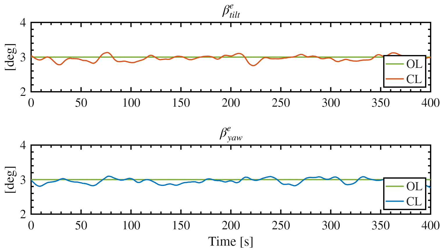
Figure 14 The comparison of pitch inputs in the helix frame between the open-loop (OL₃) and closed-loop (CL₃) cases under turbulence. Compared to OL₃, the pitch inputs of CL₃ are more dynamic.

However, a slight increase in overall power production is observed, largely attributed to the upstream turbine. This can be explained by the comparison of the pitch input signals in Fig. 14, which shows that the closed-loop controller achieves a lower time-averaged magnitude despite more dynamic inputs. Specifically, the time-averaged magnitudes of ${\mathit{\beta }}_{\mathrm{tilt}}^e$ and ${\mathit{\beta }}_{\mathrm{yaw}}^e$ are 2.95 and 2.93, respectively, compared to the constant value of 3 in the open-loop case. As established by Taschner et al. (2023), this reduction in average pitch magnitude improves upstream power production. This demonstrates that incorporating wake measurements allows the controller to reduce unnecessary actuation compared to a fixed input, thereby enhancing overall performance and supporting the value of closed-loop wake control.

Regarding structural loads, the flapwise DEL increases for the downstream turbine and the farm overall, whereas the edgewise DEL remains nearly unchanged. This result is consistent with van Vondelen et al. (2023), who noted the lower sensitivity of edgewise DEL to variations in helix magnitude.

4.3.3 Combined shear and turbulence

In the combined shear and turbulence scenario, the closed-loop system effectively corrects the shear-induced steady-state bias, though it does not fully mitigate the additional turbulence-induced oscillations. This correction facilitates enhanced wake mixing, leading to increased power production for the downstream turbine and the wind farm overall. However, these gains come at the cost of higher fatigue and a power reduction in the upstream turbine.

Compared to the open-loop baseline (OL₄), the hub vortex in the closed-loop case (CL₄) exhibits larger oscillations. This behavior can be explained by two primary reasons. The first reason is the higher time-averaged pitch actuation of 3.06 (${\overline{\mathit{\beta }}}_{\text{tilt}}^e$) and 3.03 (${\overline{\mathit{\beta }}}_{\text{yaw}}^e$) due to the increased control effort required to simultaneously correct the shear-induced bias and the attempt to stabilize turbulence-induced oscillations. The second reason is the close relationship between enhanced wake recovery and premature vortex breakdown, a phenomenon supported by the findings of Hodgson et al. (2023) and Gambuzza and Ganapathisubramani (2023). Consequently, the increased hub vortex oscillations in CL₄ may be explained by this accelerated vortex breakdown. While these results are promising, further fluid dynamics studies are necessary to fully characterize this phenomenon. Finally, the power gain in this combined case is larger than that observed in the shear-only case (CL₂), as the inherent natural mixing from the turbulence further accelerates the wake recovery process.

These observations demonstrate the closed-loop framework's efficacy in correcting shear-induced steady-state bias while simultaneously highlighting its performance boundaries under high-frequency turbulence. These results establish the technical feasibility of the controller but also show several practical trade-offs. To bridge the gap between simulations and field deployment, the following section provides a detailed discussion on the practical implementation and broader implications of the proposed framework.

5 Discussion

The previous contents of this paper demonstrate the feasibility of incorporating wake measurement in closed-loop active wake mixing control. However, some imposed assumptions imply that modifications are required before adopting the proposed framework in reality. Therefore, this section serves as a discussion of practical concerns of the trade-off between power production and load increase and the potential of integrating the wake measurement.

The simulation results presented in Sect. 4 indicate that the proposed framework has the best performance under turbulence, where an increase in power production is accompanied by a minor increase in fatigue load. However, the significant increase in fatigue load when shear is present indicates that a balance needs to be found between increasing power production and fatigue load. Although such an increase in power may be attractive to operators during periods of high electricity prices, the accompanying growth in fatigue loads must be carefully considered. Under shear conditions, the increased fatigue load of the upstream turbine can be explained by the additional pitch movement generated to correct the shear-induced steady-state bias. However, the mechanism leading to the increased fatigue load for the downstream turbine remains unknown. Therefore, further study should be conducted to understand this behavior.

Lastly, these findings yield two insights. First, the proposed framework may be better deployed under turbulent wind conditions rather than shear-dominated conditions. Furthermore, our initial strategy of moving the helix center back to the uniform open-loop counterpart may not be optimal. To improve the performance of the proposed framework under shear, further studies should therefore be conducted to examine the effect of shifting the helix center to different positions and assess how these choices influence the wind farm's performance and the corresponding operation cost. These analyses would ultimately support a more balanced wind farm performance.

6 Conclusions

This study proposed a framework for closed-loop wake mixing control, with a focus on the helix approach. A downwind-facing continuous-wave lidar is used to sample the hub vortex as the controlled variable, and a control system is designed to track the target hub vortex position in the helix frame. Simulations show that the framework performs as intended in uniform-wind conditions and shows effectiveness for the downstream turbine when shear is involved. In the latter case, the controller successfully compensates for the steady-state bias in the hub vortex trajectory, resulting in a power increase of 4.3 % and 12.6 % for the downstream turbine under shear and combined shear–turbulence conditions. Performance is limited under turbulence due to a controller roll-off induced by non-minimum-phase zeros. Nevertheless, wake-measurement-informed pitch adjustments yield modest upstream and farm-level power gains with minimal load increases, reinforcing the value of incorporating wake measurement for closed-loop control. Thus, the framework offers a novel flow-informed strategy for wake mixing control.

Future work can proceed along several perspectives. First, the proposed framework should be validated using a more realistic lidar model and in a higher-fidelity simulation environment. This enables a thorough analysis and understanding of the proposed framework. Moreover, the results presented in this paper are obtained from a single simulation with one wind seed, as this study primarily aims to serve as a proof of concept to demonstrate the feasibility of incorporating flow information into dynamic wake mixing control. Future work should therefore consider simulations with multiple wind seeds to mitigate the influence of numerical randomness and to provide a more comprehensive characterization of wind farm behavior. To balance the power production and fatigue load, simulations with more turbine settings and different wind seeds should be conducted to evaluate the balance between energy and fatigue load. Additionally, the choice of reference signal needs to be further studied to guarantee the feasibility and optimality of the wind farm performance under different wind conditions. Moreover, controllers that take the actuator and structural constraints into consideration can be designed to mitigate the increased loading on the upstream turbine. To further improve the overall performance and fully utilize the potential of the proposed framework, future works should consider conducting better feature extraction and performing quantitative flow analysis, similar to the study of Yalla et al. (2025), to directly facilitate wake mixing and better understand the influence of the proposed framework on wind flow. Simultaneously, the framework's adaptivity to naturally varying wind fields can be enhanced by integrating real-time inflow estimation techniques, such as BEM-based methods (Bertelè et al., 2017; Larsen et al., 2005), ensemble Kalman filters (Doekemeijer et al., 2017), or immersion and invariance estimators (Liu et al., 2021). Finally, it is recommended to explore integrating the proposed framework with existing methods for wake mixing to enable closed-loop control. For example, combine this study with phase synchronization (van Vondelen et al., 2025a) to enable a more adaptive application.

Appendix A: The lidar system

A lidar measures the wind speed based on the “Doppler effect” with different scanning configurations. Figure A1 illustrates the working mechanism of a single-beam measurement device: the sent and reflected wavelengths are compared, and the Doppler effect is used to derive the wind speed (Mikkelsen, 2014). The same analysis can be expanded to a multi-beam device; the main difference is that measurements along the beam are also taken into consideration by a weight function. A primary limitation of wind lidar systems is that they measure only the component of the wind velocity along the laser beam’s direction, referred to as the line-of-sight (LOS) velocity, denoted by u_LOS (Raach et al., 2017).

The scanning configuration of a lidar refers to how the laser beams scan the space to get information. There are two types of lidar applied in the field of WFFC:

1. Continuous-wave lidar shoots a continuous beam of light into the atmosphere, focusing on a predetermined distance ahead. Hence, this type of lidar only measures the wind field information at a specific distance.

2. Pulsed lidar uses a timing-based method that waits for the reflected light to return at different times after a pulse of light is emitted from the lidar. This pattern enables the measurement of wind speeds at various distances.

The work of Köpp et al. (2005) compared wake–vortex measurement quality between continuous-wave and pulsed lidar and found them to be nearly equivalent. The key distinction is that pulsed lidar samples multiple ranges at different return times, enabling analysis of the temporal evolution of vortex circulation, whereas continuous-wave lidar measures at a single focal distance, so all measurements share the same return time.

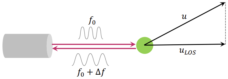
Figure A1 A simplified illustration that demonstrates the working mechanism of a single-beam measurement based on the Doppler effect. Here, f₀ and f₀+Δf denote the frequency of the sent and received waves, u denotes the wind velocity, and u_LOS denotes the line-of-sight component of the wind velocity.

The modeling of lidar in this work follows the following assumptions:

1. The half-cone angle φ of the lidar is configured to encompass the information of the entire plane with a diameter that is the same as that of the rotor disk D.

2. The focal distance of the lidar is the same as the diameter of the rotor disk D.

3. A plane can be considered a collection of many points; when a lidar measures information about a plane, it effectively samples data from these individual points by emitting multiple laser beams. Furthermore, it is assumed that these laser beams are emitted simultaneously with no phase delay.

The lidar measurement can be modeled by a point measurement in the wind field (Raach et al., 2017). In the inertial coordinate system, this is done by projecting the wind vector in three directions $u=\left[\begin{array}{ccc}{u}_{i,x}& u_{i,y}& u_{i,z}\end{array}\right]$ onto the normalized laser vector in the ith point $\left[\begin{array}{ccc}{x}_i& y_i& z_i\end{array}\right]$ with focus distance $f_i=\sqrt{x_i^{\mathrm{2}}+y_i^{\mathrm{2}}+z_i^{\mathrm{2}}}$ by

$$\begin{array}{}\text{(A1)}& u_{\mathrm{LOS},i}={\displaystyle \frac{x_i}{f_i}}{u}_{i,x}+{\displaystyle \frac{y_i}{f_i}}{u}_{i,y}+{\displaystyle \frac{z_i}{f_i}}{u}_{i,z}.\end{array}$$

In the last part of this appendix, we discuss the practical concern of using lidar. The lidar adopted in this study assumed perfect wake acquisition 1 rotor diameter downstream of the upstream turbine. However, real lidar systems may violate those assumptions, introducing various sources of uncertainty to the wake measurement. The work of Hsieh et al. (2021) compares the wake measurement of a simulated lidar and a real lidar. Overall, the study finds that the simulated lidar is able to capture the trend of the wake successfully. However, the accuracy of the lidar's measurement in the wake deficit and turbulence intensity decreases near the center of the wake due to the time and spatial averaging effect. Additionally, the work of Simley et al. (2014) demonstrates that the weight function and line-of-sight measurement introduce range weighting errors and a directional bias error, further reducing the wake measurement accuracy. Finally, the instrument-related errors of a realistic lidar, such as height-resolution limitations and environmental influences, compromise the wake measurement, as denoted by Courtney et al. (2008). As a result, the proposed pipeline needs to be retuned when applying the proposed framework with a realistic lidar. It is highly recommended to perform a field calibration before adopting the proposed framework in practice.

Appendix B: The helix transform

For ease of implementation, this work decouples the transform T(ω_rt+ω_et) as shown in van Vondelen et al. (2025b). This process starts with the sum of the angles by using the angle sum identity matrix as shown by Eq. (B1):

$$\begin{array}{}\text{(B1)}& \begin{array}{rl}\left[\begin{array}{c}\cos ({\mathit{\omega }}_{r}t+{\mathit{\omega }}_{\mathrm{e}}t)\\ \sin ({\mathit{\omega }}_{r}t+{\mathit{\omega }}_{\mathrm{e}}t)\end{array}\right]& =\left[\begin{array}{cc}\cos \left({\mathit{\omega }}_{\mathrm{e}}t\right)& -\sin \left({\mathit{\omega }}_{\mathrm{e}}t\right)\\ \sin \left({\mathit{\omega }}_{\mathrm{e}}t\right)& \cos \left({\mathit{\omega }}_{\mathrm{e}}t\right)\end{array}\right]\\ & \cdot \left[\begin{array}{c}\cos \left({\mathit{\omega }}_{r}t\right)\\ \sin \left({\mathit{\omega }}_{r}t\right)\end{array}\right]\text{.}\end{array}\end{array}$$

Subsequently, Eq. (5) can be rewritten as Eq. (B2) with R(ω_et) being the rotation matrix:

$$\begin{array}{ll}{\displaystyle }\left[\begin{array}{c}{\mathit{\beta }}_{\mathrm{col}}^e\\ {\mathit{\beta }}_{\mathrm{tilt}}^e\\ {\mathit{\beta }}_{\mathrm{yaw}}^e\end{array}\right]& {\displaystyle }=\underset{R\left({\mathit{\omega }}_{\mathrm{e}}t\right)}{\underbrace{\left[\begin{array}{ccc}\mathrm{1}& \mathrm{0}& \mathrm{0}\\ \mathrm{0}& \cos \left({\mathit{\omega }}_{\mathrm{e}}t\right)& -\sin \left({\mathit{\omega }}_{\mathrm{e}}t\right)\\ \mathrm{0}& \sin \left({\mathit{\omega }}_{\mathrm{e}}t\right)& \cos \left({\mathit{\omega }}_{\mathrm{e}}t\right)\end{array}\right]}}\\ {\displaystyle }& {\displaystyle }\times \underset{T\left({\mathit{\omega }}_{r}t\right)}{\underbrace{{\displaystyle \frac{\mathrm{2}}{\mathrm{3}}}\cdot \left[\begin{array}{ccc}\mathrm{1}/\mathrm{2}& \mathrm{1}/\mathrm{2}& \mathrm{1}/\mathrm{2}\\ \cos {\mathit{\psi }}_{\mathrm{1}}& \cos {\mathit{\psi }}_{\mathrm{2}}& \cos {\mathit{\psi }}_{\mathrm{3}}\\ \sin {\mathit{\psi }}_{\mathrm{1}}& \sin {\mathit{\psi }}_{\mathrm{2}}& \sin {\mathit{\psi }}_{\mathrm{3}}\end{array}\right]}}\\ \text{(B2)}& {\displaystyle }& {\displaystyle }\cdot \left[\begin{array}{c}{\mathit{\beta }}_{\mathrm{1}}\\ {\mathit{\beta }}_{\mathrm{2}}\\ {\mathit{\beta }}_{\mathrm{3}}\end{array}\right]\text{.}\end{array}$$

Consequently, the helix frame transform is implemented simply by multiplying a rotation matrix R(ω_et) by the MBC transform, allowing the original non-rotating frame to rotate at a frequency of ω_e rad s⁻¹, thereby making the previously rotating hub vortex stationary in the helix frame. Conversely, the inverse helix frame transformation can be derived as shown by Eq. (B3), noting that the azimuth offset ψ_off is added to decouple the tilt and yaw channels (Mulders et al., 2019):

$$\begin{array}{ll}{\displaystyle }\left[\begin{array}{c}{\mathit{\beta }}_{\mathrm{1}}\\ {\mathit{\beta }}_{\mathrm{2}}\\ {\mathit{\beta }}_{\mathrm{3}}\end{array}\right]& {\displaystyle }=\underset{T^{-\mathrm{1}}({\mathit{\omega }}_{r}t+{\mathit{\psi }}_{\mathrm{off}})}{\underbrace{\left[\begin{array}{ccc}\mathrm{1}& \cos ({\mathit{\psi }}_{\mathrm{1}}+{\mathit{\psi }}_{\mathrm{off}})& \sin ({\mathit{\psi }}_{\mathrm{1}}+{\mathit{\psi }}_{\mathrm{off}})\\ \mathrm{1}& \cos ({\mathit{\psi }}_{\mathrm{2}}+{\mathit{\psi }}_{\mathrm{off}})& \sin ({\mathit{\psi }}_{\mathrm{2}}+{\mathit{\psi }}_{\mathrm{off}})\\ \mathrm{1}& \cos ({\mathit{\psi }}_{\mathrm{3}}+{\mathit{\psi }}_{\mathrm{off}})& \sin ({\mathit{\psi }}_{\mathrm{3}}+{\mathit{\psi }}_{\mathrm{off}})\end{array}\right]}}\\ \text{(B3)}& {\displaystyle }& {\displaystyle }\times \underset{R^{-\mathrm{1}}\left({\mathit{\omega }}_{\mathrm{e}}t\right)}{\underbrace{\left[\begin{array}{ccc}\mathrm{1}& \mathrm{0}& \mathrm{0}\\ \mathrm{0}& \cos \left({\mathit{\omega }}_{\mathrm{e}}t\right)& \sin \left({\mathit{\omega }}_{\mathrm{e}}t\right)\\ \mathrm{0}& -\sin \left({\mathit{\omega }}_{\mathrm{e}}t\right)& \cos \left({\mathit{\omega }}_{\mathrm{e}}t\right)\end{array}\right]}}\cdot \left[\begin{array}{c}{\mathit{\beta }}_{\mathrm{col}}^e\\ {\mathit{\beta }}_{\mathrm{tilt}}^e\\ {\mathit{\beta }}_{\mathrm{yaw}}^e\end{array}\right]\text{.}\end{array}$$

Appendix C: Internal model identification

To identify the model, the pseudo-random binary noise (PRBN) is selected as the excitation signal due to its effectiveness in exciting a broad spectrum of system frequencies, facilitating a comprehensive capture of the system’s dynamic characteristics (Godfrey, 1991). The magnitude of the signal is set to 1°. Additionally, the signal is filtered by a bandpass filter between a frequency range of [0,0.03] Hz to ensure compatibility with the actuator's bandwidth. Furthermore, optimized predictor-based subspace identification (PBSID-opt) is used. This method is based on the well-established stochastic subspace identification approach, which uses input–output data to estimate a linear model by persistently exciting the system with an input signal containing a wide range of frequencies (van der Veen et al., 2013). The sizes of past and future windows are set identically to 200 to achieve a balance among computational speed, noise sensitivity, and accuracy. Analysis of the singular values produced by the PBSID-opt method shows a noticeable drop beyond order 4, indicating that a model of order 4 appropriately captures the spectral characteristics of the input–output data. This order offers a balance between model fidelity and computational complexity. An azimuth offset of ψ_off=6° is applied to facilitate decoupling, as it yields diagonal elements of the RGA matrix close to 1, indicating a well-decoupled system.