Adaptive economic wind turbine control

Model predictive control (MPC) for wind turbines offers several interesting advantages over simpler techniques, as for example the direct optimization of a goal function, the inclusion of constraints, non-linear coupled dynamics, and wind preview (when available). To enable real-time execution, MPC uses a reduced-order model (ROM) that approximates the dynamics of the controlled system using only a limited number of degrees of freedom. As a result, the accuracy of the ROM is often the main limit to the performance of MPC. To address this problem, an adaptive controller-internal model can reduce plant-model mismatches, potentially leading to improved performance.

This work proposes an adaptive economic non-linear MPC (ENMPC) for wind turbines. The controller maximizes profit by optimally balancing fatigue damage cost with revenue due to power generation. The cyclic fatigue cost is formulated directly in the controller using the novel parametric online rain flow counting (PORFC) approach. PORFC provides a rigorous continuous expression of the discontinuous cyclic fatigue cost using time-varying parameters. Adaptivity is obtained by a controller-internal gray-box model that combines reduced-order physical dynamics with data-driven correction terms. These are implemented via a neural network that is trained offline. Additionally, system state and disturbance estimators are included in the closed-loop controller.

The improvement in state predictions due to model adaptation is first assessed and compared with the non-adapted baseline ROM in open loop. The performance of the adaptive ENMPC and the impact of a reduced plant-model mismatch is then assessed in closed loop for a reference multi-MW onshore wind turbine in a realistic simulation environment. Results show that the adaptive ENMPC yields higher economic profits at significantly lower pitch and torque travels compared to the baseline non-adaptive ENMPC. While the enhanced closed-loop performance and economic gains of the proposed model adaptation are significant, they come at the cost of a slight increase in the computational burden of the controller.

1 Introduction

1.1 Beyond power maximization: economic wind turbine control

Wind turbine operation and control have recently shifted from the traditional goal of power maximization to more economically driven goals. In this new paradigm, turbines are operated with damage awareness in mind (Njiri and Söffker, 2016; Barradas-Berglind and Wisniewski, 2016; Loew and Bottasso, 2022; Anand et al., 2022; Loew et al., 2023). This shift is driven by the impact of fatigue damage, which shortens the operational life of turbines, and increases operation and maintenance (O&M) costs. In fact, these factors are critical to the economic profitability of operators of wind energy assets (Canet et al., 2021; Stehly et al., 2020).

One widely used method for developing economic controllers for wind turbines is model predictive control (MPC) (Rawlings et al., 2017). MPC optimizes control actions over the short-term future by predicting system behavior, and then solving an economic optimization problem based on these predictions (Rawlings et al., 2012). Existing literature shows that economic MPC formulations for wind turbine control – using the conventional objective of maximizing revenue from power generation – achieve better performance than baseline controllers and standard MPC approaches (Pustina et al., 2022; Gros and Schild, 2017; Hovgaard et al., 2015; Gros, 2013; Yan et al., 2013). However, when considering wind energy systems, an economic optimization should balance the conflicting objectives of maximizing revenue from power generation and of minimizing the cost of fatigue-related damage. Additionally, a controller should always guarantee that the system operates within feasible limits. The effectiveness of the controller ultimately depends on the quality of the solution of this constrained optimization, which essentially relies not only on the economic model but also on the quality of predictions of the controller-internal model.

1.2 The challenge of including fatigue in control formulations

The existing literature on the economic control of wind turbines using MPC is based on two main approaches for estimating cyclic fatigue: indirect and direct methods.

The indirect approach uses a proxy for fatigue (Barradas-Berglind and Wisniewski, 2016). This method is convenient because it avoids the use of cycle counting that, because of its branching nature, introduces discontinuities in the calculations (Loew et al., 2021). As a result, with the indirect approach, gradient-based methods can be used to solve the optimization problem. However, this also means that fatigue is only approximatively taken into account through a proxy quantity, which might not always provide for accurate results.

The direct approach, on the other hand, estimates fatigue explicitly using online cycle counting directly in the MPC framework (Loew et al., 2020b; Anand et al., 2022). This method, termed parametric online rain flow counting (PORFC), is relatively new and was first introduced in our previous work Loew et al. (2020a). It has since been applied in its fundamental form in various contexts, including wind turbine fatigue control (Loew et al., 2020b), battery cyclic aging control (Loew et al., 2021), and control of grid-connected wind-battery hybrid systems (Anand et al., 2021, 2022). To the authors' knowledge, PORFC is the only approach that allows for the rigorous treatment of fatigue, as it was designed to produce the same results on receding horizons that would be obtained by cycle counting the whole response time history a posteriori (Loew et al., 2020a).

1.3 The challenge of relying on controller-internal models of reduced complexity

In both approaches mentioned above, the controller relies on an internal model of the wind turbine to predict its behavior over the MPC horizon. However, due to computational effort and time constraints, the internal representation of the system response is typically obtained through a reduced-order model (ROM). ROMs approximate the system dynamics using a limited number of degrees of freedom (DOFs), enabling the real-time execution of the controller. The accuracy of these predictions plays a crucial role in the performance of the controller. A closer match between the predicted and actual wind turbine dynamics allows for the controller to make more precise decisions when optimizing the objective function, while at the same time ensuring compliance with system constraints. In fact, the degree of model mismatch not only affects optimality but may also impact the ability of the closed-loop system to operate strictly within admissible or desired limits.

One way to address model mismatches is by using state observers and estimators (Anand et al., 2022; Loew and Bottasso, 2022), where measurements of the response of the wind turbine from previous time steps are used to estimate and adjust the initialization of the controller for the next step. However, the effectiveness of this approach is limited when estimates are obtained from underlying models of scarce accuracy.

A more compelling alternative is to adapt the internal model dynamics of the controller, either by using measured operational data or synthetic results from models of sufficiently high fidelity that can accurately represent the plant behavior. One of the aims of this paper is to develop practical methods for enabling adaptivity in wind turbine ROMs.

1.4 Offline adaptation for certifiable learning control

Data-driven adaptation can be implemented online, offline, or in a hybrid manner, each of these options offering distinct trade-offs in terms of advantages, challenges, and practical applicability to economic control.

Online adaptation allows for quickly adjusting model behavior in real time based on observed plant response. However, for industrial applications, it is difficult to imagine how one could guarantee the correct learning of model corrections and how such a system could be demonstrated to always be safe and certifiable in practice.

In contrast, offline adaptation allows for the systematic integration of data, enabling a rigorous verification and validation of any learned correction terms prior to their deployment in the field. A rigorous offline verification and validation opens the door to the certification of adaptive controllers, which must meet strict standards in performance, safety, and reliability before deployment in real-world operations.

In the context of economic MPC, offline model adaptation can be achieved in several ways: by adjusting the parameters of the ROM (Schreiber et al., 2020), by incorporating a correction term into the ROM or MPC optimization function (Bottasso et al., 2006; Collet et al., 2021; Soloperto et al., 2022), or by a combination of both methods.

It is, however, important to note that a ROM captures only selected aspects of the behavior of the plant – and does so only with limited accuracy. As a consequence, the tuning of ROM parameters alone is often insufficient and may even produce non-physical results, because parameter tuning cannot compensate for missing physics. Instead, data can be leveraged to learn and incorporate the missing physics into the internal model used by the controller. This is the approach followed in this work.

The few existing studies on adaptive economic MPC for wind turbine control focus primarily on the tuning of controller gains (Shaltout et al., 2018; Tang et al., 2023). These works rely on simplified linearized models and Bayesian optimization techniques to achieve robust performance under uncertain and varying wind conditions, but they do not explicitly address model mismatch. More in general, gain tuning cannot compensate for missing or inaccurate representation of relevant physics. Recent contributions to economic MPC introduce more complex, non-linear internal models (Pustina et al., 2022, 2025); however, these approaches still lack adaptive mechanisms that explicitly compensate for modeling errors.

Furthermore, although the economic optimization in all of these studies incorporates profit-related objectives, it relies solely on indirect penalization of system states and does not explicitly account for fatigue damage, whose relevance has been highlighted by Loew and Bottasso (2022) and Anand et al. (2022).

1.5 Toward model-adaptive fatigue-aware economic wind turbine control

The key contribution of this work is the development of a novel fatigue-aware economic non-linear model predictive controller (ENMPC) with offline-adaptive capabilities enabled by data-learned ROM corrections.

The controller maximizes profit by balancing two competing factors: revenue from power generation and costs associated with fatigue damage of the turbine components. The cost of cyclic damage is formulated using the novel PORFC approach, which performs online rain flow analysis over the stress history and its future predictions to generate time-varying parameters. These parameters are then used to obtain a continuous expression of the discontinuous fatigue cost, which is incorporated into the MPC optimization. The profit formulation used here does not explicitly incorporate the effects of fatigue on component reliability and O&M costs, simply because of a lack of data and appropriate models linking loads with failure rates, instead representing fatigue-related costs solely through the amortization of the overall component cost, as discussed in TotalControl (2022).

The controller-internal model is a gray box that combines reduced-order physical dynamics with offline-computed correction terms. These terms are formulated as neural networks trained on high-resolution measured or synthetic data of the wind turbine. Their objective is to reduce model mismatch, thereby improving online closed-loop performance.

The paper is structured as follows. Section 2 introduces the proposed model adaptation approach. It describes both the simplified wind turbine model used as internal ROM and the data-driven modeling of the correction term. Section 3 provides a detailed formulation of the ENMPC, discussing various aspects of the underlying optimization problem. This section also describes the state and wind speed estimators, which provide initial conditions and disturbance predictions for the ENMPC. Section 4 presents and discusses the results from a case study. The analysis begins with an open-loop assessment of the model adaptation approach, followed by a closed-loop evaluation of its impact on economic performance, actuator usage, and computational burden. Additionally, this section examines the benefits of the proposed model adaptation under different wind input and preview scenarios. Section 5 summarizes the key findings of this work and outlines potential directions for future research.

2 Model adaptation

The proposed model adaptation approach enhances the ROM dynamics by introducing a data-driven correction function ΔF_ROM(⋅). This function is designed to compensate for the mismatch between the ROM and the actual wind turbine behavior. The adapted model dynamics, denoted as ${\mathit{F}}_{{\mathrm{ROM}}_{\mathrm{aug}}}(\cdot )$, can be expressed as

$$\begin{array}{}\text{(1)}& \dot{\mathit{x}}\left(t\right)={\mathit{F}}_{\mathrm{ROM}}\left(\mathit{x}\right(t),\mathit{u}(t),\mathit{d}(t\left)\right)+\mathbf{\Delta }{\mathit{F}}_{\mathrm{ROM}}\left(\mathit{x}\right(t),\mathit{u}(t),\mathit{d}(t),\mathit{p}),\end{array}$$

where F_ROM(⋅) represents the original non-linear ROM dynamics. By adding the corrective function ΔF_ROM(⋅), the adapted model more accurately captures the behavior of the plant. Here, x(t), u(t), and d(t) represent the continuous system states, control variables, and external disturbances, respectively. The correction ΔF_ROM depends on these same quantities but also on free parameters p that are learned based on data.

2.1 Reduced-order model

A simplified wind turbine model with only 3 degrees of freedom (drivetrain angular speed, and tower fore-aft and side-side deflections) is considered to represent the ROM dynamics F_ROM(⋅). The incident wind V_w induces an aerodynamic torque Q_a about the rotor axis and an aerodynamic force F_T along it. The aerodynamic torque directly excites the drivetrain rotational dynamics

$$\begin{array}{}\text{(2)}& J_{\mathrm{r}}\dot{\mathit{\omega }}=Q_{\mathrm{a}}-Q_{\mathrm{g}},\end{array}$$

ignoring mechanical losses, where J_r, ω, and Q_g represent the rotor moment of inertia, rotor speed, and generator torque referred to the low-speed shaft, respectively. The aerodynamic force F_T, coupled with the drivetrain dynamics, excites oscillations in the tower. These can be quantified by using the tower-top deflections in the fore-aft (noted $d_{T_{\mathrm{FA}}}$) and side-side (noted $d_{T_{\mathrm{SS}}}$) directions, which are governed by the following equations of dynamic equilibrium:

$$\begin{array}{}\text{(3a)}& {\displaystyle }{\ddot{d}}_{T_{\mathrm{FA}}}={\displaystyle \frac{\mathrm{1}}{{\mathbb{f}}_{\mathrm{1}}}}(F_{T_{\mathrm{FA}}}-{\mathbb{f}}_{\mathrm{2}}{\dot{d}}_{T_{\mathrm{FA}}}-{\mathbb{f}}_{\mathrm{3}}{d}_{T_{\mathrm{FA}}}),\text{(3b)}& {\displaystyle }{\ddot{d}}_{T_{\mathrm{SS}}}={\displaystyle \frac{\mathrm{1}}{{\mathbb{s}}_{\mathrm{1}}}}(F_{T_{\mathrm{SS}}}-{\mathbb{s}}_{\mathrm{2}}{\dot{d}}_{T_{\mathrm{SS}}}-{\mathbb{s}}_{\mathrm{3}}{d}_{T_{\mathrm{SS}}}-{\mathbb{s}}_{\mathrm{4}}{Q}_{\mathrm{g}}).\end{array}$$

Tower oscillations result in cyclic stresses σ_FA and σ_SS, respectively, at tower base. Here, $F_{T_{\mathrm{FA}}}$ and $F_{T_{\mathrm{SS}}}$ represent the rotor-plane-orthogonal (thrust) and rotor-in-plane (side-side force) components of the aerodynamic force F_T, whereas 𝕗₁₋₃ and 𝕤₁₋₄ are model parameters. The aerodynamic torque $Q_{\mathrm{a}}(\mathit{\omega },{\mathit{\beta }}_{\mathrm{b}},(V_{\mathrm{w}}-{\dot{d}}_{T_{\mathrm{FA}}}\left)\right)$ and force components $F_{T_{\mathrm{FA}}}(\mathit{\omega },{\mathit{\beta }}_{\mathrm{b}},(V_{\mathrm{w}}-{\dot{d}}_{T_{\mathrm{FA}}}\left)\right)$ and $F_{T_{\mathrm{SS}}}(\mathit{\omega },{\mathit{\beta }}_{\mathrm{b}},(V_{\mathrm{w}}-{\dot{d}}_{T_{\mathrm{FA}}}\left)\right)$ introduce non-linearities in the model.

The turbine model has two control variables: the commanded generator torque Q_gc and the commanded blade pitch angle β_c. The dynamics of the generator is given as

$$\begin{array}{}\text{(4)}& {\dot{Q}}_{\mathrm{g}}={\displaystyle \frac{\mathrm{1}}{{\mathbb{g}}_{\mathrm{1}}}}(Q_{\mathrm{gc}}-Q_{\mathrm{g}}),\end{array}$$

where coefficient 𝕘₁ represents the time-constant of the first-order dynamic model. The pitch dynamics is modeled as

$$\begin{array}{}\text{(5)}& {\ddot{\mathit{\beta }}}_{\mathrm{b}}=-{\mathbb{b}}_{\mathrm{1}}{\dot{\mathit{\beta }}}_{\mathrm{b}}-{\mathbb{b}}_{\mathrm{2}}({\mathit{\beta }}_{\mathrm{b}}-{\mathit{\beta }}_{\mathrm{c}}).\end{array}$$

Here, β_b represents the effective collective blade pitch angle, and the coefficients 𝕓₁₋₂ are model parameters representing properties of the second-order pitch model.

The reduced-order wind turbine model consists of eight system states

$$\begin{array}{}\text{(6)}& \mathit{x}=(\mathit{\omega },d_{T_{\mathrm{FA}}},{\dot{d}}_{T_{\mathrm{FA}}},d_{T_{\mathrm{SS}}},{\dot{d}}_{T_{\mathrm{SS}}},{\mathit{\beta }}_{\mathrm{b}},{\dot{\mathit{\beta }}}_{\mathrm{b}},Q_{\mathrm{g}}),\end{array}$$

and two control input variables

$$\begin{array}{}\text{(7)}& \mathit{u}=({\mathit{\beta }}_{\mathrm{c}},Q_{\mathrm{gc}}).\end{array}$$

The wind speed V_w is considered as the single disturbance input to the model, i.e.,

$$\begin{array}{}\text{(8)}& \mathit{d}=V_{\mathrm{w}}.\end{array}$$

The reduced-order model outputs the wind turbine electrical power

$$\begin{array}{}\text{(9)}& P_{\mathrm{gen}}={\mathit{\eta }}_{\mathrm{gen}}\mathit{\omega }{Q}_{\mathrm{g}}\end{array}$$

and the tower-base stresses

$$\begin{array}{}\text{(10)}& {\mathit{\sigma }}_{\mathrm{FA}/\mathrm{SS}}={\mathbb{t}}_{\mathrm{1}}{d}_{T_{\mathrm{FA}/\mathrm{SS}}}\end{array}$$

in the fore-aft and side-side directions, modeled as linear functions of the respective tower-top deflections. Here, η_gen denotes the drivetrain conversion efficiency, and 𝕥₁ is a constant of proportionality derived from the tower-base geometry and material properties.

2.2 Data-driven correction

With advancements in computing technologies, machine learning techniques – including supervised and unsupervised learning – have become highly effective for a wide range of data-driven system identification tasks. A key advantage of supervised learning over unsupervised learning is its access to both input states and their corresponding target states during training. This allows the model to generalize and predict system behavior for previously unseen input combinations. A particularly effective approach for supervised learning in this context is based on the training of a neural network (NN). NNs can approximate arbitrarily complex functions while also providing gradients, making them especially well suited for integration in an optimal control framework.

In this work, the NN is designed to provide a static mapping from inputs to outputs. The network architecture consists of multiple hidden layers and a single output layer, with each layer composed of a certain number of neurons. Each neuron is defined by weights, biases, and an activation function. Within a given layer, the input data is first transformed by applying the weights and biases associated with the neuron. The resulting weighted sums are then passed to the next layer through the selected activation function. Activation functions apply a non-linear mapping to the weighted input plus bias, which determines whether and to what extent a neuron is activated, thereby enabling the network to model complex, non-linear relationships between inputs and outputs. The choice of activation function therefore plays a key role in shaping the flow of information through the network and, consequently, its predictive performance. Moreover, for use in an ENMPC, the activation function must be continuous and differentiable, so that first- and second-order derivatives can be computed. These derivatives are required for the numerical solution of the underlying optimization problem by gradient-based methods (Rawlings et al., 2017).

A feed-forward NN with one hidden layer and one output layer is considered in this work. The static mapping of the input features x_NN to the output features y_NN for the considered NN can be written as

$$\begin{array}{}\text{(11)}& {\mathit{y}}_{\mathrm{NN}}={\mathit{f}}_y^{\mathrm{act}}\left({\mathbf{W}}_y^T{\mathit{f}}_h^{\mathrm{act}}\right({\mathbf{W}}_h^T{\mathit{x}}_{\mathrm{NN}}+{\mathit{b}}_h)+{\mathit{b}}_y).\end{array}$$

Here, W, b, and f^act(⋅) represent the weights, biases, and activation functions, respectively, where the subscript h denotes the hidden layer and the subscript y denotes the output layer.

Before training the NN, the generated dataset is split into training and testing sets. Moreover, every feature in the input and the target set is normalized by subtracting the minimum of the feature vector from the feature vector itself, and then dividing the result by the range (difference of maximum and minimum), i.e.:

$$\begin{array}{}\text{(12)}& {\mathit{y}}_{\mathrm{NN}}={\displaystyle \frac{{\mathit{y}}_{\mathrm{NN}}-{\mathit{y}}_{\mathrm{NN}}^{min}}{{\mathit{y}}_{\mathrm{NN}}^{max}-{\mathit{y}}_{\mathrm{NN}}^{min}}}.\end{array}$$

Furthermore, the normalized datasets are shuffled to reduce the possible clustering of conditions that might create biases. After preprocessing the training set, the parameters p of the NN, defined as

$$\begin{array}{}\text{(13)}& \mathit{p}=({\mathbf{W}}_h,{\mathit{b}}_h,{\mathbf{W}}_y,{\mathit{b}}_y),\end{array}$$

are computed using the Levenberg–Marquardt algorithm to minimize the sum of squares of error between the predicted output and target output.

The accuracy of NN predictions depends heavily on the quality of its training process, which requires a comprehensive dataset of inputs and corresponding target outputs. Wind turbine original equipment manufacturers (OEMs) typically have validated high-fidelity models from design and prototyping that can generate representative datasets, and they may also have access to high-resolution data from on-board sensors of operational turbines to supplement them. In the present work, data are obtained from a high-fidelity simulation model, using both standard measurements and estimates derived from these measurements.

Figure 1 illustrates the proposed approach of acquiring input and target data for NN training, where the solid blue circles represent the plant states ${\mathit{x}}_i^{\mathrm{Plant}}$ at a given time instant i. To generate training data, the ROM is initialized with each plant state sample, setting ${\mathit{x}}_i^{\mathrm{ROM}}={\mathit{x}}_i^{\mathrm{Plant}}$. The ROM then predicts the next state ${\mathit{x}}_{i+\mathrm{1}}^{\mathrm{ROM}}$, based on the applied control inputs ${\mathit{u}}_i^{\mathrm{Plant}}$ and the influence of external disturbance ${\mathit{d}}_i^{\mathrm{Plant}}$.

Figure 1 Data acquisition for model adaptation.

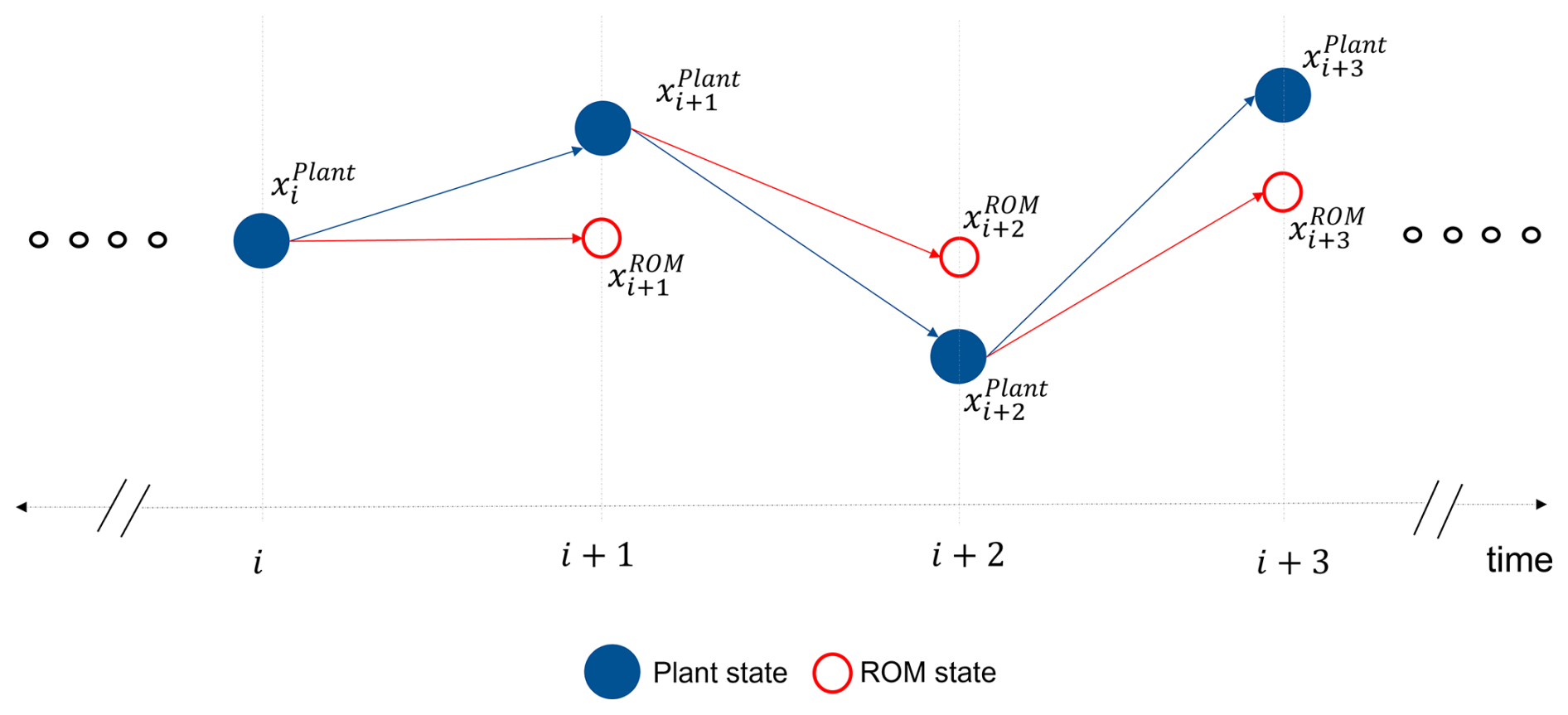
The error between the derivatives of the ROM model and the plant is defined as

$$\begin{array}{}\text{(14)}& {\mathit{e}}_{i+\mathrm{1}}={\dot{\mathit{x}}}_{i+\mathrm{1}}^{\mathrm{Plant}}-{\dot{\mathit{x}}}_{i+\mathrm{1}}^{\mathrm{ROM}},\end{array}$$

and constitutes the target dataset. Derivatives are calculated using the current state ${\mathit{x}}_i^{\mathrm{Plant}}$ at time t_i and the corresponding next states ${\mathit{x}}_{i+\mathrm{1}}^{\mathrm{Plant}}$ and ${\mathit{x}}_{i+\mathrm{1}}^{\mathrm{ROM}}$ at time t_i+1 via finite differences, i.e. $({\mathit{x}}_{i+\mathrm{1}}-{\mathit{x}}_i)/(t_{i+\mathrm{1}}-t_i)$. The set of the current states, control inputs, and disturbances applied to the plant constitutes the input dataset $({\mathit{x}}_i^{\mathrm{Plant}},{\mathit{u}}_i^{\mathrm{Plant}},{\mathit{d}}_i^{\mathrm{Plant}})$ for the ith time sample. This simple temporal discretization, although of limited numerical accuracy, is deemed sufficient for the present application, where modeling errors are typically larger than the numerical ones.

3 ENMPC formulation

The ENMPC is formulated based on the augmented internal model ROM_aug, as expressed by Eq. (1), to predict the system states and associated outputs over a short future horizon T_horizon. The discretization of time-continuous variables is performed over the prediction horizon using N_u control time steps of duration $T_{\mathrm{ctrl}}=T_{\mathrm{horizon}}/N_u$. The predictions of states and outputs are used to calculate control inputs that optimize a desired meaningful economic objective function (here chosen as profit, with the goal of balancing revenue and costs). Moreover, constraints are enforced to the optimization problem to ensure that the controller keeps the plant states and applied inputs within feasible ranges.

The proposed ENMPC optimization problem is formulated as

$$\begin{array}{}\text{(15a)}& \begin{array}{rl}\underset{\mathit{u},\mathit{\xi }}{min}& -(J_{\mathrm{generation}}^{\mathrm{Power}}{)}^{\mathrm{2}}+(J_{\mathrm{tower}\mathrm{fatigue}}^{\mathrm{FA}}{)}^{\mathrm{2}}+(J_{\mathrm{tower}\mathrm{fatigue}}^{\mathrm{SS}}{)}^{\mathrm{2}}\\ & +\underset{t_{\mathrm{0}}}{\overset{t_{\mathrm{0}}+T_{\mathrm{horizon}}}{\int }}(W_{\mathrm{1}}^{\mathit{\xi }}{\mathit{\xi }}_{\mathrm{1}}^{\mathrm{2}}+W_{\mathrm{2}}^{\mathit{\xi }}{\mathit{\xi }}_{\mathrm{2}}^{\mathrm{2}})\mathrm{d}t,\end{array}\end{array}$$

subject to

$$\begin{array}{}\text{(15b)}& {\displaystyle }{\dot{\mathit{x}}}_{\mathrm{c}}={\mathit{F}}_{{\mathrm{ROM}}_{\mathrm{aug}}}({\mathit{x}}_{\mathrm{c}},\mathit{u},\mathit{d},\mathit{p}),\text{(15c)}& {\displaystyle }\underset{\mathrm{¯}}{\mathit{u}}\le \mathit{u}\le \stackrel{\mathrm{‾}}{\mathit{u}},\text{(15d)}& {\displaystyle }\underset{\mathrm{¯}}{\mathit{x}}\le \mathit{x}\le \stackrel{\mathrm{‾}}{\mathit{x}},\text{(15e)}& {\displaystyle }\underset{\mathrm{¯}}{\mathit{\xi }}\le \mathit{\xi }\le \stackrel{\mathrm{‾}}{\mathit{\xi }},\text{(15f)}& {\displaystyle }\underset{\mathrm{¯}}{{\dot{Q}}_{\mathrm{g}}}\le {\dot{Q}}_{\mathrm{g}}\le \stackrel{\mathrm{‾}}{{\dot{Q}}_{\mathrm{g}}}.\end{array}$$

The meaning of all variables and terms in this problem are explained in Sect. 3.1–3.3.

3.1 Optimization variables

The optimization variables in the problem expressed by Eq. (15a)–(15f) are the control inputs $\mathit{u}=({\mathit{\beta }}_{\mathrm{c}},Q_{\mathrm{gc}})$ and the slack variables $\mathit{\xi }=({\mathit{\xi }}_{\mathrm{1}},{\mathit{\xi }}_{\mathrm{2}})$. The purpose of introducing slack variables is to achieve recursive feasibility of the MPC optimization problem in the presence of model uncertainties and system perturbations (Gros, 2013). Hence, in the present formulation, the state variable ω and the output variable P_gen are augmented using the bounded slack variables ξ₁ and ξ₂, respectively. This approach is used because ω, despite the smoothing effect provided by the large rotor inertia, is subject to wind perturbations and model errors that affect the economic MPC problem (Gros, 2013). The modified set of states x_c is expressed as

$$\begin{array}{}\text{(16)}& {\mathit{x}}_{\mathrm{c}}=(\mathit{\omega }+{\mathit{\xi }}_{\mathrm{1}},d_{T_{\mathrm{FA}}},d_{T_{\mathrm{SS}}},{\mathit{\beta }}_{\mathrm{b}},{\dot{\mathit{\beta }}}_{\mathrm{b}},Q_{\mathrm{g}},P_{\mathrm{gen}}+{\mathit{\xi }}_{\mathrm{2}}).\end{array}$$

3.2 Optimization objective

The optimization objective aims to maximize the generated profit by maximizing the revenue accrued from wind power generation and minimizing the cost incurred due to fatigue damage. The cost of fatigue damage should be expressed by appropriate models, which will differ depending on the component; for example, it is reasonable to assume that the effects of cyclic loading on a pitch bearing will in general be very different from the ones on a gearbox. Here, for the lack of specific models and relevant data, we simply consider the tower as an exemplary component that is often fatigue critical. It is clear that this is only an academic example, and more realistic scenarios could be readily developed by using the same methodology for multiple components using dedicated component-specific cost models.

The wind power generation is maximized by considering the aerodynamic power capture

$$\begin{array}{}\text{(17)}& J_{\mathrm{generation}}^{\mathrm{Power}}=w_P\underset{t_{\mathrm{0}}}{\overset{t_{\mathrm{0}}+T_{\mathrm{horizon}}}{\int }}\left(\mathit{\omega }{Q}_{\mathrm{a}}\right(\mathit{\omega },{\mathit{\beta }}_{\mathrm{b}},(V_{\mathrm{w}}-{\dot{d}}_{T_{\mathrm{FA}}})\left)\right)\mathrm{d}t,\end{array}$$

where w_P denotes the revenue rate for providing electricity to the grid. It should be noted that even though revenue is accrued based on the overall electrical power generation, in this work the aerodynamic power is maximized. This is to avoid the greedy extraction of rotor kinetic energy by MPC (referred to as “turnpike effect” in Gros, 2013).

In general, the revenue rate w_P depends on time, because time-dependent ambient conditions influence the energy mix and because market prices may vary dynamically. However, the typical time scales of these variations are much longer – usually on the order of tens of minutes and specifically 15 min in intra-day markets – than the receding horizon used in MPC, which typically spans only a few seconds. For this reason, even though w_P appears outside the integral in Eq. (17), the present formulation remains fully applicable to variable electricity prices.

The tower cyclic fatigue damage is minimized by a direct penalization of fatigue via the PORFC approach. The PORFC algorithm uses a preprocessing step to identify fatigue cycles c for a given set of stress samples σ and splits the respective cyclic fatigue damages over the contributing samples. In the general case, a particular stress sample may belong to no cycle (when it is not an extremum), one cycle (when it is part of only one half or full cycle), or two cycles (when it lies at a cycle-junction point) (Shi et al., 2018, 2019). The output of the preprocessing step is the PORFC mean parameters ${\mathit{\sigma }}_{m,c}^{\mathrm{PORFC}}$ and PORFC weight parameters ${\mathit{\sigma }}_{w,c}^{\mathrm{PORFC}}$ (Loew et al., 2021).

A Python script to extract the PORFC parameters for a given set of stress trajectories is shared with this work (Anand and Bottasso, 2025). This allows for a detailed understanding of the novel formulation, and its adaptability and usage for economic MPC. The script performs standard rain flow counting to identify cycle characteristics and extract PORFC parameters. These parameters are then used to reformulate the cycle amplitudes and weights over stress samples in a continuous manner.

The cost of tower fatigue damage $J_{\mathrm{tower}\mathrm{fatigue}}^{\mathrm{FA}}$, due to tower root fore-aft cyclic stress σ_FA, is formulated as

$$\begin{array}{}\text{(18a)}& {\displaystyle }{J}_{\mathrm{tower}\mathrm{fatigue}}^{\mathrm{FA}}={\displaystyle \frac{\mathrm{1}}{T_{\mathrm{ctrl}}}}\underset{t_{\mathrm{0}}}{\overset{t_{\mathrm{0}}+T_{\mathrm{horizon}}}{\int }}\sum _{c=\mathrm{1}}^{\mathrm{2}}{J}_{c,{\mathit{\sigma }}_{\mathrm{FA}}}^{\mathrm{PORFC}}({\mathit{\sigma }}_{\mathrm{FA}},{\mathit{\sigma }}_{\mathrm{FA}m,c}^{\mathrm{PORFC}},{\mathit{\sigma }}_{\mathrm{FA}w,c}^{\mathrm{PORFC}})\mathrm{d}t,\text{(18b)}& {\displaystyle }{J}_{c,{\mathit{\sigma }}_{\mathrm{FA}}}^{\mathrm{PORFC}}={\mathit{\sigma }}_{\mathrm{FA}w,c}^{\mathrm{PORFC}}{a}_{\mathbb{m}}{\mathit{\sigma }}_{\mathrm{FA}\mathrm{eq},c}^{\mathbb{m}},\text{(18c)}& {\displaystyle }{\mathit{\sigma }}_{\mathrm{FA}\mathrm{eq},c}=|{\mathit{\sigma }}_{\mathrm{FA}}-{\mathit{\sigma }}_{\mathrm{FA}m,c}^{\mathrm{PORFC}}|{\displaystyle \frac{R_{\mathbb{m}}}{R_{\mathbb{m}}-{\mathit{\sigma }}_{\mathrm{FA}m,c}}}.\end{array}$$

Here, a_𝕞 denotes the capital cost of the component and is determined from the initial capital expenditure of the machine (see also Loew et al., 2023, for details), R_𝕞 denotes the ultimate tensile strength of the material, and 𝕞 represents the positive exponent derived from the material S-N characteristic.

The tower cyclic fatigue damage $J_{\mathrm{tower}\mathrm{fatigue}}^{\mathrm{SS}}$, due to tower root side-side cyclic stress σ_SS, is formulated in a similar manner.

Although the optimization objective, shown in Eq. (15a), separately considers the costs of tower fore-aft and side-side fatigue, the final evaluation is based on the projected total cost, as explained below. In addition to the fact that fore-aft and side-side components depend on wind direction, which is not constant, this also ensures that any potential increase or decrease in tower side-side stress oscillations resulting from control actions aimed at minimizing tower fore-aft stress (and vice versa) is properly accounted for.

To obtain the cost of cyclic fatigue damage for each projection at a given azimuth direction on a tower section, the following steps are taken. First, rain flow counting is performed on the projected stress trajectory. Then, the Goodman equation is applied for mean stress correction. The damage cost of each stress cycle is determined using the S-N curve of the material of the tower and the component cost. Finally, the Miner–Palmgren algorithm is used to sum the costs of individual cycles and obtain the total cost; refer to Loew et al. (2023) for a detailed description of this formulation.

This approach – here illustrated for the tower – is readily generalized to other components. Once cyclic fatigue is assessed on each prediction horizon for each component of interest, a dedicated model could provide failure rates and/or maintenance activities resulting from such loading, in turn generating the associated costs, which would be included in the optimization merit function.

It should be noted that the objective terms of the optimization problem are not assigned arbitrary or heuristic weights. Instead, each term is weighted according to its actual economic value. As a result, the optimization outcomes are economically meaningful and directly aligned with practical decision-making considerations, rather than being influenced by ad hoc tuning of weights. For instance, the weighting term to calculate revenue due to power production is represented by the (optionally time-varying) revenue rate w_P, as shown in Eq. (17). Similarly, the cost due to accumulated tower fatigue damage is weighted using the initial capital-cost parameter a_m through the online rain flow analysis, as shown in Eq. (18a–18c).

3.3 Optimization constraints

The ENMPC optimization problem expressed by Eq. (15a)–(15f) is subjected to various constraints.

The equality constraints expressed by Eq. (15b) enforce the governing equations of the augmented plant-model ROM_aug(⋅) and have the role of informing the problem of the underlying system dynamics.

The optimization is also subjected to inequality constraints. To ensure feasible states and control inputs, box constraints are provided through Eq. (15c) and (15e), respectively. Slack variables are bounded using Eq. (15d) to ease convergence. Finally, the rate of change of generator torque ${\dot{Q}}_{\mathrm{g}}$ is bounded using Eq. (15f) to reduce torque travel and fatigue in the drivetrain.

3.4 Estimators

3.4.1 State estimator

The controller-internal model is initialized using the currently measured initial states x₀. However, not all system states of the internal model can actually be measured directly on the plant using standard on-board sensors. For instance, both the tower-top deflection and velocity states ($d_{T_{\mathrm{FA}}}$, ${\dot{d}}_{T_{\mathrm{FA}}}$,$d_{T_{\mathrm{SS}}}$, ${\dot{d}}_{T_{\mathrm{SS}}}$) for ROM and ROM_aug cannot be measured directly on a real turbine. Only the rotor speed ω, the blade pitch angle β_b, and the tower-top accelerations ${\ddot{d}}_{T_{\mathrm{FA}}}$ and ${\ddot{d}}_{T_{\mathrm{SS}}}$ can be measured by on-board sensors, whereas the remaining states need to be estimated using measured quantities. Furthermore, as the controller-internal model is only a reduced representation of the plant, the initial values measured directly on the plant may not be suitable for initializing the ENMPC. As a consequence, a state estimator is additionally required to provide initial value estimates x_est of the system states for the ENMPC internal model, using the available measurements from the plant.

A classical approach for state estimation is the Kalman filter, also widely used for wind turbine control (Bottasso and Croce, 2009; Ritter, 2020). However, due to the non-linear nature of the system and the need to enforce constraints on both stage and terminal states, here we instead adopt a moving horizon estimator (MHE). A detailed comparison between optimization-based state estimation techniques based on MHE and Kalman filters has been presented in Loew and Bottasso (2022). The MHE formulation used in this study builds upon the approach discussed in Anand et al. (2022).

MHE utilizes system information from the plant over a finite past horizon, noted as T_horizon,est, to calculate the initial state estimates x_est(t₀) for the current ENMPC step. The MHE optimization problem is formulated as

$$\begin{array}{}\text{(19a)}& {\displaystyle }\begin{array}{rl}\underset{\overline{\mathit{\nu }}}{min}& \underset{t_{\mathrm{0}}-T_{\mathrm{horizon},\mathrm{est}}}{\overset{t_{\mathrm{0}}}{\int }}\left(\right||{\mathit{x}}_{\mathrm{est}}-{\mathit{x}}_{\mathrm{est},\mathrm{prev}}|{|}_{{\mathbf{W}}_{\mathrm{prev}}}^{\mathrm{2}}+\left|\right|{\mathit{y}}_{\mathrm{est}}\\ & -{\mathit{y}}_{\mathrm{meas}}|{|}_{{\mathbf{W}}_{\mathrm{meas}}}^{\mathrm{2}}+|\left|\overline{\mathit{\nu }}\right|{|}_{{\mathbf{W}}_{\overline{\mathit{\nu }}}}^{\mathrm{2}})\mathrm{d}t,\end{array}\text{(19b)}& {\displaystyle }\text{subject to}\text{(19c)}& {\displaystyle }{\dot{\mathit{x}}}_{\mathrm{est}}={\mathit{F}}_{\mathrm{est}}\left({\mathit{x}}_{\mathrm{est}}\right(t),{\mathit{d}}_{\mathrm{est}}(t\left)\right)+\overline{\mathit{\nu }}\left(t\right).\end{array}$$

The objective function is represented by the weighted sum of the squares of state and output deviations, and of the noise variable $\overline{\mathit{\nu }}$ (Gros, 2013; Huang et al., 2010). The diagonal weighting matrices W_meas, W_prev, and ${\mathbf{W}}_{\overline{\mathit{\nu }}}$ are obtained by a trial and error tuning, such that a satisfactory performance is achieved.

The role of the state deviation term is to ensure a smooth estimator output over consecutive MHE steps.

The estimated and measured outputs are respectively defined as ${\mathit{y}}_{\mathrm{est}}=({\mathit{x}}_{\mathrm{est}},{\ddot{d}}_{T_{\mathrm{FA},\mathrm{est}}},{\ddot{d}}_{T_{\mathrm{SS},\mathrm{est}}})$ and ${\mathit{y}}_{\mathrm{meas}}=({\mathit{x}}_{\mathrm{meas}},{\ddot{d}}_{T_{\mathrm{FA},\mathrm{meas}}},{\ddot{d}}_{T_{\mathrm{SS},\mathrm{meas}}})$. The estimated tower-top fore-aft acceleration ${\ddot{d}}_{T_{\mathrm{FA},\mathrm{est}}}$ and side-side acceleration ${\ddot{d}}_{T_{\mathrm{SS},\mathrm{est}}}$ are obtained using the non-linear output equation expressed by Eq. (3a) and (3b), respectively. The measured tower-top fore-aft acceleration ${\ddot{d}}_{T_{\mathrm{FA},\mathrm{meas}}}$ and the side-side acceleration ${\ddot{d}}_{T_{\mathrm{SS},\mathrm{meas}}}$ are obtained from the plant as a result of standard sensor measurements. The measured tower-top velocity and deflection in both the fore-aft and side-side directions are obtained by numerical integration of the tower-top acceleration and velocity, respectively.

The optimization problem is subjected to the equality constraints expressed by Eq. (19c), which inform the estimator of the underlying system dynamics. In Eq. (19c), ${\mathit{d}}_{\mathrm{est}}\left(t\right)=\left(V_{\mathrm{w}}\right(t),{\mathit{\beta }}_{\mathrm{b}}(t),Q_{\mathrm{g}}(t\left)\right)$ are the disturbance inputs to the system, which are already set by the ENMPC and are hence fixed for the current MHE step. Here, x_est represents the estimator system states, corresponding to the wind turbine system states x, as discussed in Sect. 2.1. Moreover, F_est(⋅) represents the system of ODEs for wind turbine dynamics discussed in Sect. 2.1.

After the execution of an MHE step, the terminal state at the end of the MHE horizon becomes the initial state at the beginning of the ENMPC prediction horizon, i.e. ${\mathit{x}}_{\mathrm{0}}=\mathit{x}\left(t_{\mathrm{0}}\right)={\mathit{x}}_{\mathrm{est}}\left(t_{\mathrm{0}}\right)$.

3.4.2 Disturbance estimator

The wind speed V_w is considered as a disturbance input to the ENMPC formulation and needs to be estimated over the prediction horizon T_horizon of the controller. This work considers a simple rotor-effective wind speed (REWS) estimator, based on the approach discussed in Soltani et al. (2013). The REWS estimator utilizes the drivetrain dynamics, expressed by Eq. (2), to estimate the aerodynamic torque as

$$\begin{array}{}\text{(20)}& {Q_{\mathrm{a}}}_{\mathrm{est}}={\displaystyle \frac{{P_Q}_{\mathrm{est}}}{{\mathit{\omega }}_{\mathrm{meas}}}}\approx {\displaystyle \frac{{P_{\mathrm{gen}}}_{\mathrm{meas}}+J_{\mathrm{r}}\dot{\mathit{\omega }}}{{\mathit{\omega }}_{\mathrm{meas}}}},\end{array}$$

where ${P_{\mathrm{gen}}}_{\mathrm{meas}}$ is the measured generator power and ω_meas is the measured rotor speed. The rate of change of rotor speed $\dot{\mathit{\omega }}$ is computed by finite difference from ω_meas. The estimated aerodynamic torque ${Q_{\mathrm{a}}}_{\mathrm{est}}$ is then equated to the aerodynamic torque $Q_{\mathrm{a}}({\mathit{\omega }}_{\mathrm{meas}},{{\mathit{\beta }}_{\mathrm{b}}}_{\mathrm{meas}},{V_{\mathrm{w}}}_{\mathrm{est}})$, described in Sect. 2.1, to estimate wind speed ${V_{\mathrm{w}}}_{\mathrm{est}}$ for the measured pitch angle ${{\mathit{\beta }}_{\mathrm{b}}}_{\mathrm{meas}}$ and ω_meas.

4 Results and discussions

4.1 Case study

The ability of the adapted model to accurately predict the plant states depends directly on the precision of the data-driven corrections. Additionally, to determine the extent of model adaptation required, it is necessary to assess how reducing the model mismatch influences the closed-loop performance of the controller. To answer these questions, we consider a plant represented by the NREL 5 MW reference wind turbine (Jonkman et al., 2009), which is modeled using OpenFAST (Jonkman et al., 2022), a widely used tool for simulating wind turbine dynamics.

The plant model includes the first and second flapwise, and the first edgewise bending modes for each of the three blades. Additionally, it also includes the first and second tower bending modes in both fore-aft and side-side directions, as well as the torsional flexibility of the drivetrain and the generator DOF.

The model, which incorporates pitch and torque actuators but excludes the yaw mechanism, consists of 33 system states. There are eight states for the tower dynamics, 18 for the blades (six per blade), two for drive-shaft torsion, two for rotor rotation, two for collective blade pitch actuation, and one for generator torque actuation.

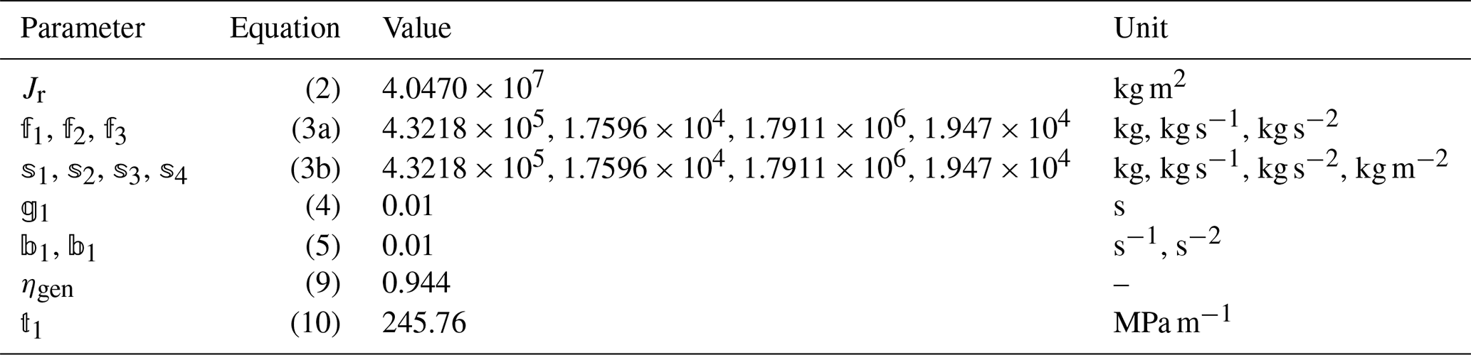
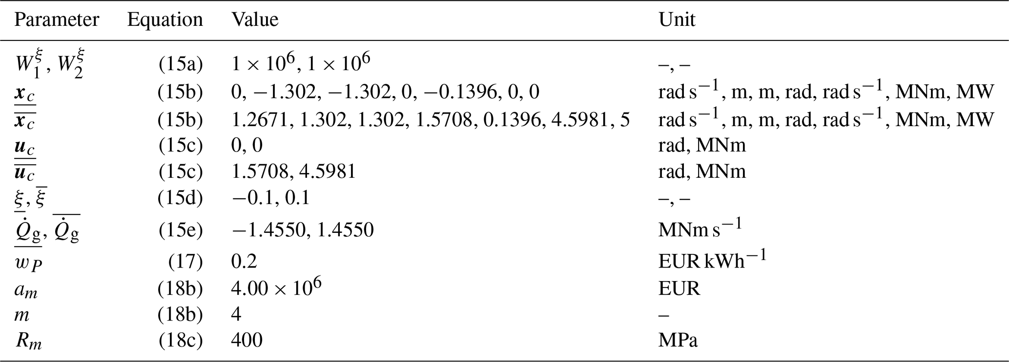
The fixed model parameters of the corresponding ROM, namely 𝕗₁₋₃, 𝕤₁₋₄, 𝕘₁, 𝕓₁₋₂, and 𝕥₁, are derived from the NREL report describing the 5 MW reference wind turbine (Jonkman et al., 2009). Table 1 summarizes these parameters and lists their corresponding values.

Table 1 ROM parameters derived from the 5 MW reference wind turbine report and OpenFAST baseline-controller simulations (Jonkman et al., 2009).

4.1.1 Data generation

The performance of an NN depends heavily on the quality of its training, which requires an exhaustive dataset that encompasses a wide range of operating conditions. To generate a comprehensive training dataset, the OpenFAST model is simulated in turbulent wind conditions using the baseline controller provided in the OpenFAST package. Full-field turbulent wind inputs are generated using TurbSim (Jonkman, 2009), considering the class-B normal turbulence model. Simulations are performed for wind speeds ranging from cut-in to cut-out in 1 m s⁻¹ steps. For each wind speed, six different turbulent wind seed simulations are conducted.

Figure 2 presents the Pearson correlation coefficients of the states (x), inputs (u), and disturbances (d) of the ROM with the corresponding state errors (refer to Sect. 2.2), computed over the entire dataset. The Pearson correlation coefficient quantifies the linear relationship between two variables (Faizi and Alvi, 2023). Each entry in the table of Fig. 2 displays the absolute value of the coefficient, where a higher magnitude indicates a stronger correlation. The same relationship is visualized through a color gradient map, where darker shades represent stronger correlations and lighter shades indicate weaker ones.

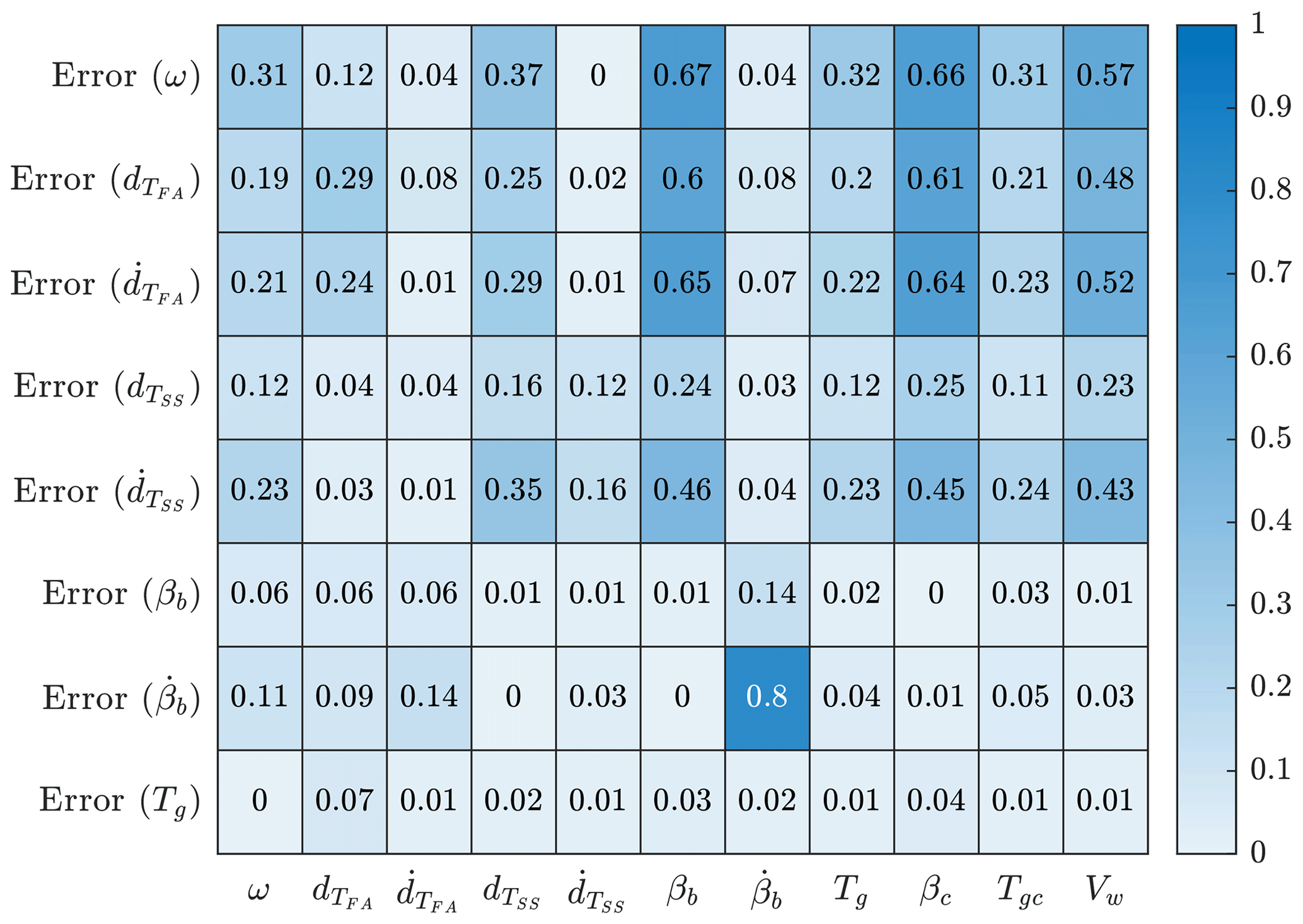
Figure 2 Correlation coefficient of states, inputs, and disturbance of the controller-internal model (as columns) with the error in states (as rows) for the generated dataset, rounded off to two significant digits. The number in each cell denotes the absolute value of the Pearson correlation coefficient, while the cell color visually denotes the degree of correlation.

Figure 2 shows that all ROM states and inputs significantly influence the state errors, as evidenced by their non-zero correlation coefficients. In particular, the rotor speed (ω) and blade states (${\mathit{\beta }}_{\mathrm{b}},{\dot{\mathit{\beta }}}_{\mathrm{b}}$) exhibit the strongest correlation with both rotor speed errors and tower state errors. Additionally, the control inputs (β_c and Q_gc) and wind speed (V_w) strongly affect the mismatch across all states. Furthermore, the non-zero yet distinct correlation magnitudes for blade pitch (β_b) and collective blade control (β_c) highlight the importance of blade dynamics, expressed by Eq. (5), in the internal model of the controller. This suggests that, while the ROM captures an approximation of the complex aeroelastic response, it does not fully represent the detailed dynamics present in the plant.

4.1.2 NN training

The proposed NN input set x_NN contains 11 features (eight system states, two control variables, and one disturbance input), and each output set y_NN contains eight features representing errors in the derivatives of states calculated using the plant and ROM states. The selection of input features is guided by the correlation coefficients presented in Fig. 2, which indicate a non-zero correlation between all variables in the input and target sets. The hidden layer of the network consists of 20 neurons, each utilizing a radial basis activation function, while the output layer comprises eight neurons with linear activation functions. The number of neurons in the hidden layer was determined through hyperparameter tuning, ensuring optimal training performance.

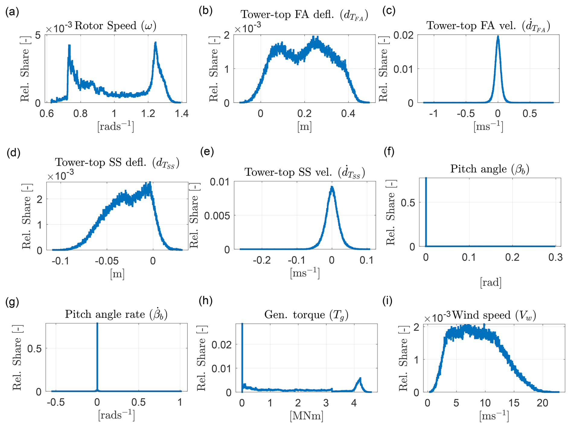
Before training the NN, the generated dataset is split into training and testing sets. During wind turbine operation, more data are naturally collected for operating conditions, corresponding to more probable wind speed values. To account for this effect in the application of the proposed methodology, the dataset split is performed according to a hypothetical site-specific Weibull distribution. Figure 3 illustrates the distribution of selected input features in the training dataset.

The various subplots in Fig. 3 show that the dataset covers a broad operational range of the wind turbine, allowing the NN to predict the target variables across a wide range of input conditions. Furthermore, Fig. 3i confirms that the wind speed distribution in the training dataset closely follows the Weibull shape, ensuring a realistic representation of operating conditions.

Figure 3 Distribution of different input features in the training set.

The training dataset consists of 216 071 sample points. This number is small compared to the number of data points typically generated for design load case (DLC) 1.2 of the IEC Standards 61400-1 applicable to wind turbine certification and testing (IEC, 2019), which – assuming six turbulence seeds and a sampling rate of 0.1 s – would result in 3 312 000 data points. This suggests that model adaption may be based on datasets that are 1 order of magnitude smaller than datasets routinely collected for standard design and certification purposes.

4.2 Open-loop evaluation

The ability of the augmented internal model to track system states accurately is essential for ensuring both the optimality and the stability of the closed-loop behavior. To evaluate this aspect of the proposed approach, both ROM_aug and ROM are simulated using each input combination from the testing dataset (refer to Sect. 4.1.2), with the initial state accordingly set. The final states predicted by both models are then compared to the corresponding plant states, and the prediction error is computed to quantify the accuracy achieved by each model.

Figure 4 presents the kernel density plot of the absolute prediction errors for both ROM (solid blue line) and ROM_aug (solid green line) across all system states. For each of the subplot, the x axis represents the absolute error values, while the y axis shows the probability density estimate (PDE), calculated using a normal kernel function.

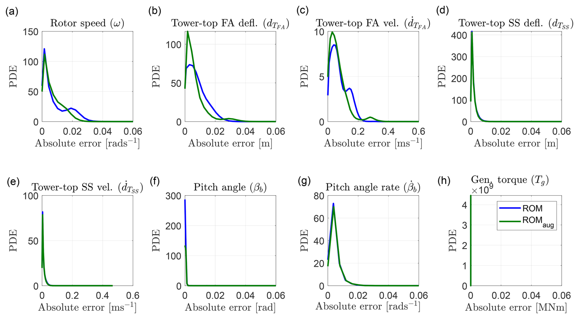
Figure 4 PDEs of the open-loop prediction errors for both ROM_aug and ROM, shown in green and blue, respectively, evaluated over the test set.

In the ROM case, certain states, such as “Tower-top FA defl.” and “Tower-top FA vel.”, exhibit their highest PDE at a non-zero error value, indicating a mismatch in model fidelity. In contrast, in the ROM_aug case, this mismatch is corrected using the proposed adaptation scheme. As a result, the PDE peak shifts toward zero, signifying an improved state prediction accuracy. Furthermore, for most system states, the PDE peak magnitude in the ROM_aug case is higher than in the ROM case. This indicates a greater concentration of cases where ROM_aug achieves lower absolute errors than ROM, further demonstrating the effectiveness of the proposed model augmentation. The figure also shows that the accuracy of some quantities cannot be improved, although their typical errors are always very small.

To quantify the effectiveness of ROM_aug in minimizing plant-model mismatch in open-loop, a statistical evaluation was conducted using the mean and standard deviation (STD) of prediction errors. Table 2 presents the percentage reduction in both the error mean and STD for ROM_aug, relative to ROM, across the test set.

Table 2 Percentage reduction in error mean and STD thanks to model augmentation, as assessed on the test set.

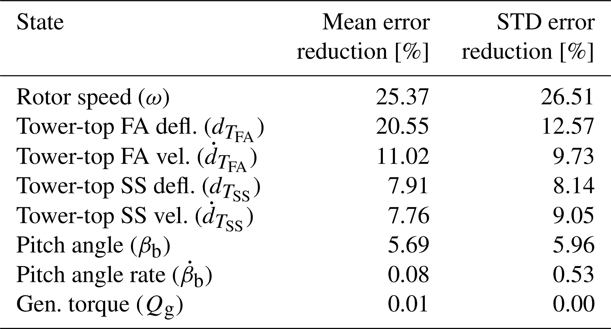
The results show varying degrees of improvement in state prediction, demonstrating that NN-based augmentation reduces not only the average error but also the error spread over different operating conditions. A greater reduction in prediction error is observed for states with higher absolute error magnitudes in Fig. 4. This highlights the effectiveness of weight tuning during the NN training stage, which prioritizes correcting states with significant errors. These findings further emphasize the effectiveness of the proposed offline data-driven approach in reducing plant-model mismatch, improving the overall accuracy of the internal model.

For a practical application of the model adaptation, it is interesting to quantify the amount of training data that are needed to achieve a desired level of performance. To this end, multiple data subsets are created from the original training set. Each subset contains a specified fraction of the data samples from the original training set.

Figure 5a illustrates the distribution of wind speed for multiple subsets, ranging from 45 % to 95 % of the original training set. The x axis represents the wind speed, while the y axis shows the corresponding relative share. Each subset is used to train an NN, with the same architecture as described in Sect. 4.1.2.

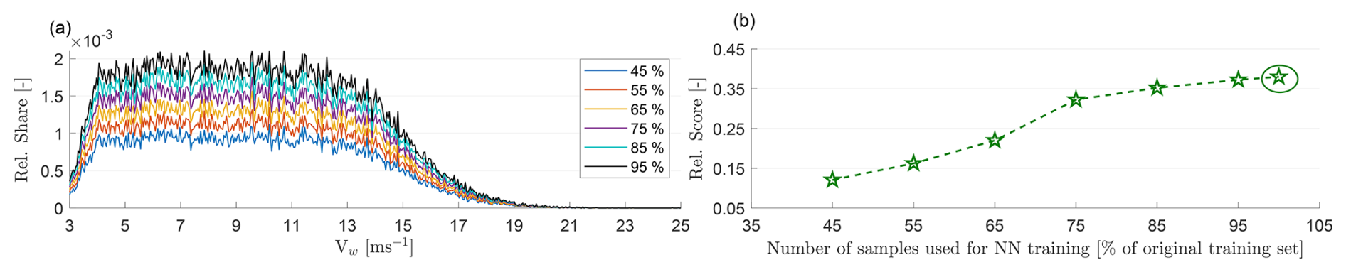
Figure 5 Open-loop evaluation of the proposed model adaptation where the NNs are trained using subsets of the full training set. Relative share of wind speed (V_w) in the NN training set (a). Corresponding performance score of ROM_aug relative to the performance score of ROM as a function of test set size (b).

Figure 5b presents the performance of the adapted models evaluated on the same test set. The performance score is calculated by summing the root mean square error (RMSE) of predictions for all eight states. The y axis reports the performance scores of the different ROM_aug models, normalized against the performance score of ROM. The x axis displays the number of samples in percentage of the full training set. The figure also reports the normalized performance score of the ROM_aug model trained with the full dataset, represented by the green circle.

The results show that, as expected, incorporating more data into the training process provides the NN with additional information, leading to improved performance. However, even a relatively small subset of training data helps to reduce the plant-model mismatch. Furthermore, performance begins to level off beyond a certain point, as additional data samples no longer significantly contribute to improving the model because they do not carry any extra useful informational content that is not already present in the data pool. In this study, performance starts to plateau once 85 % of the training dataset is used. As noted earlier, even when using the full dataset, the number of data points that are necessary for model adaption is small compared to the typical datasets collected in standard aeroelastic analyses conducted during routine design and certification activities.

4.3 Closed-loop evaluation

Although the long tail of the PDE plots in Fig. 4 indicate that the prediction errors of the augmented ROM remain non-zero for some operating conditions, it is still useful to examine the potential benefit of reducing plant-model mismatch on closed-loop performance, as this helps to quantify the necessary level of compensation. To investigate this aspect of the formulation, the proposed adaptive economic controller is implemented in closed loop with the plant. This configuration is referred to as ENMPC_aug. To assess the impact of the augmentation, the plant performance is also evaluated using the same ENMPC formulation but based on the original, non-augmented ROM, referred to as ENMPC.

Several studies on wind turbine control have demonstrated that economic MPC formulations yield superior performance compared to baseline controllers (Jonkman et al., 2009; Abbas et al., 2022), as well as standard reference-tracking-based MPC formulations. This holds both for pure power-maximization objectives (Pustina et al., 2022; Hovgaard et al., 2015; Gros and Schild, 2017; Yan et al., 2013) and for combined power-maximization and fatigue-minimization objectives (Loew and Bottasso, 2022; Soleymani et al., 2024; Wang et al., 2025). Therefore, the discussion in this section focuses only on the closed-loop behavior of ENMPC and ENMPC_aug formulations, in order to quantify the performance improvement resulting from model adaptation.

We consider DLC 1.2 at 11 m s⁻¹ wind speed. The ENMPC-MHE optimization problem (refer to Sect. 3) is solved via the state-of-the-art Acados framework (Verschueren et al., 2019). The interior-point solver HPIPM is used for solving the underlying quadratic programs (QP) in the non-linear program (NLP). Several sequential quadratic program (SQP) iterations are carried out at each controller step. The multiple shooting approach is employed with a Newton step length of 1. To address potential numerical issues caused by the highly non-standard formulation produced by PORFC (Loew et al., 2020b), the Hessian matrix is automatically convexified. It is important to note that solving multiple SQPs can improve performance. However, it also increases the computational burden.

The ENMPC and MHE horizon lengths, T_horizon and T_horizon,est, are both set to 2 s, each having 20 discretization steps. This results in a sample time T_ctrl of 100 ms for both the controller and the estimator. The sample time of the plant, T_sim, is set to 10 ms. The optimal control inputs applied to the plant model are considered as piece-wise constant values over T_ctrl. Measurements from the plant are taken every T_ctrl. Table 3 lists the fixed optimization parameters for the ENMPC. The weighting matrices for the MHE optimization are listed in Loew and Bottasso (2022).

Table 3 Fixed optimization parameters for closed-loop evaluation. The values are derived from Loew et al. (2023); Anand et al. (2022); Sutherland (1999); Jonkman et al. (2009).

The closed-loop simulations run for a duration of 10 min. Six turbulent wind speed seeds, generated using TurbSim, are used to characterize uncertainties in fatigue damage. The controller uses the estimated wind speed REWS (refer to Sect. 3.4.2) as input, which remains constant over the prediction horizon of the controller.

The closed-loop control performance is evaluated using the following performance indicators:

1. Revenue due to power generation, calculated considering a fixed feed-in tariff w_P and turbine electrical power generation η_gen ω Q_g (refer to Eq. 17 for details).

2. Cost due to projected tower-base fatigue damage. To calculate the projected damage, the tower fore-aft σ_FA(t) and tower side-side oscillations σ_SS(t) are first projected along the various azimuth directions at the tower base. Next, the fatigue damage cost is computed for each of these projections, as discussed in Sect. 3.2. Finally, the maximum cost across all projections is selected.

3. Profit, calculated as the difference of revenue and cost.

4. Pitch travel, showing the total degrees that the blades traveled for a given control formulation. This can be considered as a proxy for the usage of pitch actuators, which may be prone to wear and tear, calling for extra maintenance.

5. Torque travel, showing the total amount of torque that the generator had to apply. This can be considered as a proxy for the usage of the turbine drivetrain, leading to the wear and tear of bearings and the gearbox. Additionally, it also serves as a proxy for switching-related damage in the power electronic converters.

4.3.1 Economic performance of the controller

Figure 6 presents the performance indicators calculated over 10 min, with results averaged across different seeds. The set of bars in the left and right parts of the figure represent the performance for the ENMPC and ENMPC_aug formulations, respectively. The color of the bars corresponds to different performance indicators. The results for ENMPC_aug are normalized with the ENMPC ones to facilitate comparison. The y axis shows these relative values, which are also noted in black above each bar. Additionally, the numbers on the face of each bar, shown in purple text, represent the absolute values.

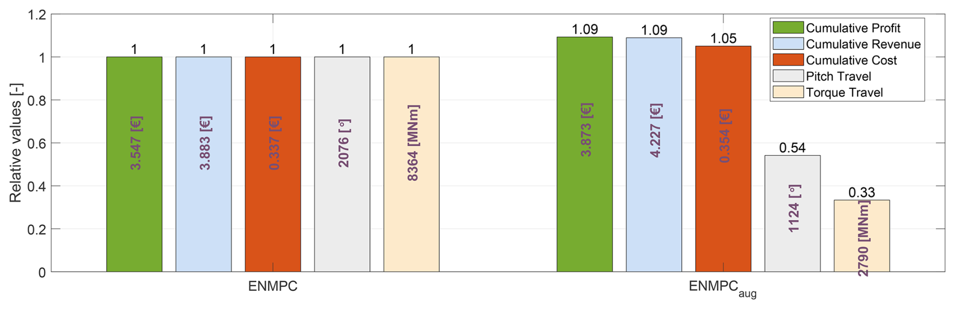
Figure 6 Performance indicators for closed-loop simulations using controllers employing the baseline ROM (ENMPC) and the augmented ROM (ENMPC_aug) as internal models. The black numbers on the top of each bar denote the corresponding relative cumulative values. The purple text on the face of each bar denotes the absolute cumulative values.

Figure 6 shows that ENMPC_aug results in 9 % higher economic profit than ENMPC. This improvement is due to the more accurate estimation of revenue and cost in ENMPC_aug, which is made possible by a better prediction of the system states. The higher profit is directly attributed to an increased revenue, with a slight increase in cost. Since the absolute economic value of revenue exceeds that of cost (as shown by the purple numbers on the face of the bars), ENMPC_aug effectively balances the two, leading to a higher overall economic profit.

In contrast, for the ENMPC case, while the controller aims to maximize economic profit, the plant-model mismatch leads to control actions that are not economically optimal. As a result, the controller struggles to accurately estimate and balance revenue and cost, ultimately resulting in a lower economic profit.

Furthermore, since the future predictions in the controller more closely match the actual evolution of the plant in the ENMPC_aug formulation, the controller requires less frequent control actions. This is reflected in the significantly smaller pitch and torque travel compared to the ENMPC case.

As a result, reducing plant-model mismatch to improve system state predictions not only enhances performance but also leads to a substantial reduction in actuator usage. It is reasonable to assume that this, in turn, will result in lower maintenance costs for both the actuators and the drivetrain. This effect was, however, not quantified here, as a result of a lack of data and of specific and reliable models.

4.3.2 Benefits under different wind inputs

Advanced wind turbine control formulations require the current wind speed as an input. Improved foresight of the wind speed enables the ENMPC to determine the most suitable control actions.

Wind speed can be gauged using a simple wind speed estimator, as utilized in this work (refer to Sect. 3.4.2), or through advanced estimators as discussed in Soltani et al. (2013). Alternatively, the current wind speed can be measured directly, either using a nacelle-mounted anemometer or a light detection and ranging (LiDaR) device. LiDaRs not only provide real-time wind speed data but also offer short-term wind speed previews. This capability makes LiDaRs an ideal complement to MPC-based wind turbine control, where the MPC optimization uses system states derived from wind speed forecasts over the MPC prediction horizon (Loew and Bottasso, 2022; Canet et al., 2021).

Here, the benefits of the proposed model adaptation for reducing plant-model mismatch under different wind input estimates are assessed. Figure 7 presents various wind profiles used as input to the controller.

Figure 7 Exemplary wind profiles used as disturbance inputs to the ENMPC formulations.

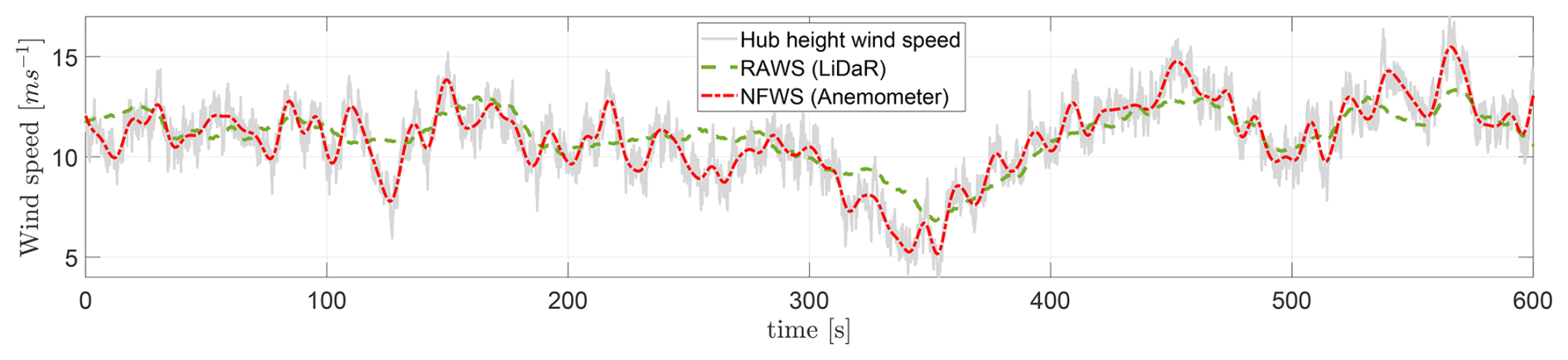
The solid gray curve represents the longitudinal component of the full wind field generated using TurbSim at the turbine hub height for a 10 min duration. This scenario is labeled “Hub height wind speed”. This is only shown to illustrate wind fluctuations, but it is not used as input to the controller. The dash-dotted red curve corresponds to the nacelle filtered wind speed (NFWS), which is a rough approximation of what an anemometer mounted on the nacelle would measure. Typically, anemometer measurements are subjected to various disturbances, including – among others – flow distortion due to proximity of the nacelle (a bluff body), periodic effects caused by blade passage, interference due to the wake, and sensor noise. For the lack of models of these complex phenomena, here we have simply filtered the wind field at the nacelle location using a standard bandpass filter. This case is referred to as “Anemometer”. The dashed green curve shows the rotor-averaged wind speed (RAWS). The RAWS is a much simplified representation of what a nacelle-mounted scanning LiDaR system with discrete scanning and spatial averaging would estimate under a frozen turbulence hypothesis, i.e., with a purely rigid transport of the flow from the measurement volume to the rotor disk (Loew and Bottasso, 2022). This case is referred to as “LiDaR”.

It can be observed that the anemometer-measured wind speed follows the highly turbulent fluctuations of the wind speed at hub height. Additionally, the RAWS shows even less dynamic variation in the wind speed but successfully captures the long-term wind speed trends. Although these speeds are only very rough approximations of the wind that could be actually measured on a wind turbine, they still capture a range of situations from point-wise exact values to spatial and temporal averages.

Figure 8 presents the results obtained with the closed-loop control formulations, considering different wind speed estimates. For each wind speed input scenario, two sets of bars are displayed: the first set represents the ENMPC case, while the second corresponds to the ENMPC_aug case. In each set, each of the five performance indicators is shown as a bar of a different face color. The various sets of bars correspond to the following situations:

• The first and second sets show results when the controllers use REWS, described in Sect. 3.4.2, as disturbance input and the current wind speed is held constant over the prediction horizon. These results are the same as discussed in Fig. 6 and are shown here again for ease of comparison.

• The third and fourth sets show results when the controllers use NFWS (Anemometer) as disturbance input and the current wind speed is held constant over the prediction horizon.

• The fifth and sixth sets show results when the controllers use LiDaR measurements as input and the current wind speed is held constant over the prediction horizon.

• The seventh and eighth sets show results when the controllers use LiDaR measurements as input and a perfect preview of wind condition over the prediction horizon is considered. This case has been labeled as LiDaR-PF.

The results are normalized with respect to the ENMPC case, which is shown in the first set. The black text above each bar represents the relative cumulative values. To aid interpretation, the results from different wind input scenarios are highlighted with distinct background colors. The red background corresponds to the Anemometer scenario, the light-green shade represents the LiDaR scenario, and the dark-green background indicates the LiDaR-PF scenario.

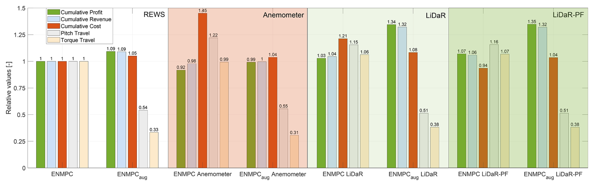
Figure 8 Performance indicators for closed-loop simulations using ENMPC and ENMPC_aug. The background colors denote different wind input scenarios: white for REWS, red for Anemometer, light-green for LiDaR, and dark-green for LiDaR-PF. For a given background color, the left and right columns show ENMPC and ENMPC_aug results, respectively. The black numbers on the top of each bar denote the corresponding relative cumulative values.

The results show that providing the controller with more accurate information about the wind disturbance input leads to an increase in economic profit for both ENMPC and ENMPC_aug. As expected, the Anemometer scenario, providing only a disturbed point-wise wind measurement, results in the lowest economic profit, while the LiDaR-PF scenario yields the highest economic profit.

Furthermore, for all wind input scenarios, the proposed model adaptation results in higher economic profit and reduced pitch and torque travel. The magnitude of the performance improvement varies across the different wind input scenarios. For example, ENMPC_aug achieves a 7 % higher economic profit in the Anemometer scenario and a 30 % increase in the LiDaR scenario, compared to the corresponding ENMPC formulation. It is noteworthy that the economic performance of ENMPC_aug in the LiDaR scenario is only slightly worse than that in the LiDaR-PF scenario. This suggests that, for this case study, a perfect wind preview does not significantly pay off, and a simple constant speed estimate is sufficient. However, a more general conclusion can only be drawn by evaluating the two scenarios over a wider range of turbine inflow conditions.

4.3.3 Computational performance

An economic controller is real-time feasible if the computational time required to generate the optimal control actions is less than the sample time of the plant. The length of the prediction horizon, along with the nature of the underlying internal model and the optimization problem, directly affects the number of SQP iterations needed for the controller to converge to a solution. A higher number of SQP iterations increases the computational time.

Although this work does not focus on optimizing the computational performance of the formulated controllers to ensure real-time feasibility, the impact of the proposed model adaptation on the computational performance of the controllers is assessed.

Figure 9 presents the economic profit and computational time for ENMPC_aug LiDaR, with the controller limited to a maximum of 3, 5, and 10 SQP iterations, as reported on the x axis. The results are normalized with respect to the ENMPC LiDaR formulation, which uses a maximum of 10 SQP iterations. The y axis on the left shows the relative economic profit in blue, while the y axis on the right displays the relative mean CPU time per controller iteration in orange. The results for ENMPC_aug LiDaR are marked with circular markers filled in blue, and the results for ENMPC LiDaR are marked with circular markers filled in green.

The simulations were performed on a desktop computer with an Intel i7 processor, a 64-bit operating system, and 8 GB of RAM.

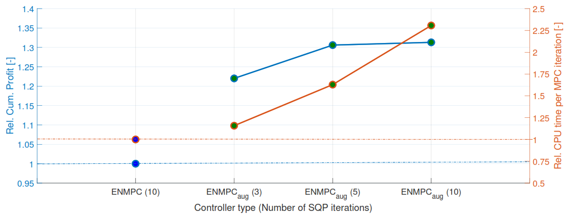
Figure 9 Economic performance and the corresponding CPU time requirement for the ENMPC_aug LiDaR formulation utilizing an increasing number of SQP iterations. Performance is normalized with respect to the ENMPC LiDaR formulation utilizing 10 SQP iterations.

The results clearly show that increasing the number of SQP iterations leads to a higher relative economic profit. For 10 SQP iterations, ENMPC_aug LiDaR results in a 30 % higher economic profit, but it requires more than double the computational effort compared to ENMPC LiDaR. This is because of the additional calculations in the NN part of the model.

Interestingly, ENMPC_aug LiDaR with only five SQP iterations still achieves a 22 % higher economic profit than ENMPC LiDaR with 10 SQP iterations, while requiring just 15 % more computational effort. This demonstrates that, although the proposed model adaptation increases the CPU time for ENMPC, the improvement in economic performance outweighs the additional computational cost. Moreover, the adapted model requires fewer SQP iterations to generate economically optimal control actions at a smaller actuator usage.

This effect, combined with the use of high-performance computational platforms and further software optimization for speed may result in real-time feasible economic controllers.

5 Conclusions

MPC uses an approximate representation of the plant to predict the system evolution over a short future horizon. The internal models used by MPC are typically a reduced representation of the plant. The resulting model mismatch affects the feasibility and the optimality of the closed-loop performance. This study presented a fatigue-aware adaptive ENMPC for closed-loop control of wind turbines. The ENMPC directly incorporates cyclic fatigue costs using a novel online rain flow counting approach and is able to generate more accurate model predictions through a data-driven adapted model.

The proposed adaptive ENMPC aims to maximize economic profit, which is here computed as the revenue from power generation minus the cost of fatigue damage at the tower base. Revenue is calculated based on the (optionally time-varying) market tariff and the energy supplied to the grid. The cyclic fatigue damage is estimated using online rain flow counting on adapted model predictions, while also accounting for residual cycles. While cycle counting is the only approach to precisely account for fatigue, it also inherently introduces discontinuities in the MPC optimization problem. To address this problem, the PORFC approach is used to externalize fatigue estimation from the MPC optimization. This method estimates time-varying fatigue-related parameters, allowing for a continuous formulation of cyclic fatigue costs that can be numerically optimized in the MPC.

The ENMPC optimization problem is subject to bound constraints on system states and control variables, ensuring feasible solutions and a stable closed-loop behavior. The ENMPC formulation is further enhanced by integrating state and disturbance estimators. These estimators account for measurement uncertainties and provide accurate initial values for the ENMPC.

The proposed approach utilizes wind turbine operational or synthetic data with machine learning techniques to predict the mismatch in the system states of plant and ROM. A data-driven model is developed to estimate the error in the states across a range of relevant inflow and control conditions. This process results in an adapted model, where the underlying dynamics are represented by a simple physics-based model combined with data-driven correction terms. The adapted ROM is then used as the internal model in the controller. This process is performed offline, which offers two important advantages. First, it does not introduce additional computational effort during operation, thereby facilitating real-time performance. Second, it results in a certifiable controller, for which safety and performance can be fully assessed offline before deployment in the field. The same is far more difficult – if possible at all – for controllers based on online learning.

The performance of the proposed approach is assessed through a case study using an OpenFAST model of the NREL 5 MW reference wind turbine as a plant. This model generates measurement data for the study. The plant model has 15 degrees of freedom and includes 33 system states, while the ROM has only 3 degrees of freedom and consists of 8 system states. The simulation data is generated across a wide range of operational conditions. A feed-forward NN is developed to predict the error in plant and ROM states, and is then used in the adapted model dynamics.

The performance of the proposed model adaptation is initially evaluated in an open-loop setup. In this case, the predictions of the adapted model ROM_aug and the baseline ROM are compared with the actual behavior of the plant across a range of operational conditions. The kernel density estimates of the prediction error show that the adapted model performs significantly better than the original model for all eight system states. The performance improvement is further quantified in terms of statistics of the prediction error. The results reveal a reduction in both the mean and standard deviation of errors for all system states, with an approximate 20 % reduction in the angular velocity error of the rotor.

Additionally, the effect of dataset size on the open-loop performance of the proposed model adaptation is assessed. Results indicate that even a relatively small subset of training data helps to reduce the plant-model mismatch. Performance starts to plateau once 85 % of the generated training dataset is used, as additional data samples no longer significantly improve the model. This amount of data is about 1 order of magnitude smaller than the number of data points typically collected during aeroelastic analyses carried out as part of routine design and certification activities.

To further quantify the impact of model adaptation on the economic control of wind turbines, the closed-loop performance of the proposed economic MPC formulation is assessed using ROM_aug as the internal model of the controller. Five performance indicators are considered: revenue (due to wind power generation), cost (due to tower fatigue damage), profit (calculated as the difference of revenue and cost), pitch travel (as a proxy for actuator usage), and torque travel (as a proxy for damage of power electronic converters and drivetrain usage).

The performance of ENMPC_aug that uses the enhanced model is compared to the ENMPC formulation that uses the baseline ROM as its internal model. Results show that ENMPC_aug achieves 9 % higher economic profit than ENMPC. This improvement is attributed to more accurate revenue and cost estimations, made possible by better predictions of the system states. Additionally, since the future predictions in ENMPC_aug are closer to the actual evolution of the plant, the controller requires relatively fewer control actions. This is reflected in a significantly smaller pitch and torque travel compared to the ENMPC formulation.

The benefits of the proposed model adaptation are further assessed across different wind input scenarios. The results show an increased economic profit with improved wind foresight for both ENMPC_aug and ENMPC. Moreover, the model adaptation leads to higher economic profit – up to 30 % in the LiDaR scenario – and reduced pitch and torque travel for all wind input scenarios.

Although this study did not focus on optimizing the computational performance of the controllers for real-time feasibility, the impact of model adaptation on computational performance was also evaluated. The results show that increasing the number of SQP iterations leads to higher economic profit but also increases computational expenses. Additionally, for the same number of SQP iterations, ENMPC_aug is more computationally expensive than ENMPC due to the extra computational cost due to NN evaluations. However, when considering LiDaR wind estimates, ENMPC_aug achieves a 22 % higher economic profit while requiring only 15 % more computational effort compared to ENMPC. Therefore, the proposed model adaptation, combined with high-performance computing platforms and additional software optimization (not considered here), could enable real-time feasible economic controllers.

The accuracy of offline data-driven model corrections depends strongly on the quality of the training process, which requires a comprehensive dataset that characterizes the range of operational conditions experienced by a wind turbine. In practice, wind turbine OEMs typically have validated high-fidelity turbine models developed during design and prototyping, and these models can be used to represent turbine behavior and generate the required dataset. Moreover, OEMs often have access to high-resolution measurements from on-board sensors of operating turbines, which can further contribute to the dataset. The generalized usability of the adapted model depends on how similar turbine behavior is across different installation sites, an aspect that has not been investigated in this work.

Future work should focus on developing a more comprehensive economic objective that accounts for fatigue damage affecting additional turbine components, such as the bearings and the drivetrain, while also incorporating a more realistic profit model. This would require applying the PORFC formulation to other fatigue-critical components of the turbine and integrating it into ENMPC as either an objective function or a constraint. The assessment can be extended to new scenarios that consider more dynamic variations of exogenous inputs, such as market prices over longer evaluation periods. At present, the profit formulation neglects the influence of fatigue on component reliability and O&M costs, and it considers only tower fatigue damage. In addition, the physics-based internal model can be expanded to capture dependencies on a wider set of system states. The model can also be improved by introducing online tuning of model parameters in addition to the offline augmentation used in this study.

Appendix A: Nomenclature and abbreviations

DLC	Design load case
DOF	Degree of freedom
ENMPC	Economic non-linear model predictive control
ENMPCaug	Economic non-linear model predictive control having ROMaug as the controller-internal model
FA	Fore-aft
LiDaR	Light detection and ranging
MHE	Moving horizon estimator
MPC	Model predictive control
NFWS	Nacelle filtered wind speed
NLP	Non-linear program
NN	Neural network
O&M	Operation and maintenance
ODE	Ordinary differential equation
OEM	Original equipment manufacturer
PDE	Probability density estimate
PF	Perfect foresight
PORFC	Parametric online rain flow counting
QP	Quadratic program
RAWS	Rotor-averaged wind speed
REWS	Rotor-effective wind speed
RMSE	Root mean square error
ROM	Reduced-order model
ROMaug	Augmented reduced-order model
SQP	Sequential quadratic program
SS	Side-side
STD	Standard deviation
ξ	Slack variable
$\overline{\mathit{\nu }}$	Noise variable
ω	Rotor speed
βb	Blade pitch angle
βc	Commanded blade pitch angle
σ	Stress at tower base
η	Power conversion efficiency of the drivetrain
F	Set of dynamic equations of a model
ΔF	Set of dynamic equations of the correction model
FT	Aerodynamic thrust force
J	Optimization objective
Jr	Moment of inertia of the rotor
Nu	Number of intervals in the controller prediction horizon
P	Electrical power output of the turbine
Qa	Aerodynamic torque
Qg	Generator torque
Qgc	Commanded generator torque
R𝕞	Ultimate tensile strength of the material

Tctrl	Sample time of the internal model and the controller
Thorizon	Prediction horizon of the controller
Thorizon,est	Prediction horizon of the state estimator
Tsim	Sample time of the plant
Vw	Wind speed
W	Weight
a𝕞	Initial capital cost of the machine
b	Bias
c	Cycle
d	Disturbance variable
$d_{T_{\mathrm{FA}}}$	Tower-top deflection in fore-aft direction
$d_{T_{\mathrm{SS}}}$	Tower-top deflection in side-side direction
e	Error in state
fact	Activation function
i	Time instant
m	Time-varying PORFC parameter: mean
p	Free model parameter
t	Time
Δt	Time step
u	Control variable
w	Time-varying PORFC parameter: weight
x	State variable
xNN	Input feature of the NN
yNN	Output feature of the NN
𝕓1−2	Model parameters for blade dynamics
𝕗1−3	Model parameters for tower fore-aft dynamics
𝕘1	Model parameters for generator dynamics
𝕞	Fatigue exponent derived from material properties
𝕤1−4	Model parameters for tower side-side dynamics
𝕥1	Model parameters for estimating tower-base stresses using tower-top deflections
□aug	Augmented
□est	Estimation
□gen	Generation
□meas	Measurement
□prev	Previous
□sim	Simulation