Generating high-fidelity wind fields from the wind speed correlation tensor

In this publication a new method to generate stochastic representations of homogeneous and isotropic wind fields is presented. In contrast to the typically employed algorithm, the new approach is based on the wind speed correlation tensor. This allows for the simulation of a homogeneous and isotropic turbulent wind field with very high accuracy, achieving a deviation of the obtained dataset's structure function from the theoretical one that is at least 1 order of magnitude lower than that of the commonly used method. A compensation method to decrease this error even further is proposed. Moreover, being a generic method, it can be used to simulate other Gaussian phenomena (e.g., temperature or index of refraction fluctuations) in various spatial domains with uniformly spaced rectangular grid shapes. The motivation for this paper is to develop an algorithm that is able to synthesize high-fidelity homogeneous and isotropic wind speed datasets within an arbitrary model domain geometry without the need for optimizing weighting parameters. This is achieved by eliminating the band-pass effect of the discrete Fourier transform inherent to the typically used algorithm.

1 Introduction

In recent decades, researchers and engineers have increasingly relied on the use of synthetic datasets to represent complex physical phenomena during the design process. Examples include the generation of wind speed along the three spatial dimensions, used in the design of airframe structures (as described in Hoblit, 1988, or in the aviation regulations, CS25, 2023) and the computation of wind turbine loads (as specified in IEC61400-1, 2019). Further, synthetic datasets are relevant for the generation of phase screens, used in modeling optical propagation through the turbulent atmosphere (Andrews and Phillips, 2005). For this reason, within the last 60 years, several stochastic synthesis methods have been developed, particularly for phenomena that are considered to be Gaussian and stationary (e.g., temperature fluctuations and homogeneous, isotropic turbulence). These methods are based on different statistical approaches, including modal decomposition techniques (Fried, 1965), autoregressive models (Baran and Infield, 1995), linear dynamical system solutions (Beghi et al., 2011), machine learning (Wold et al., 2024), or the spectral representation of the phenomenon. This last family of algorithms can be further divided into the methods computing the dataset using the relation between the phenomenon's correlation function and power spectral density (PSD) (Borgman et al., 1984); the ones embedding the correlation matrix, computed from the correlation function, into a circulant matrix from which the dataset is generated by means of eigenvalue decomposition (Dietrich and Newsam, 1993; Wood and Chan, 1994); and the ones synthesizing the dataset directly from the spectrum of the phenomenon (Mann, 1998). The latter class of algorithms, referred to in this article as the random phase method (RPM) after Wilson (1998), has been widely used in the realization of stochastic wind fields in the last 20 years (e.g., Friedrich et al., 2022; Chen et al., 2022). However, to the authors' knowledge, there is still no algorithm capable of synthesizing a high-fidelity wind field dataset (i.e., achieving a deviation from the theoretical correlation of less than 1 %) in different spatial domains (e.g., a cuboid of 2000 m × 2000 m × 2000 m or a parallelepiped of 8000 m × 500 m × 500 m) without the need for specific optimization or weighting parameters. The here-proposed method builds on the RPM and the Fourier integral method (FIM), developed by Pardo-Iguzquiza and Chica-Olmo (1993), solving the optimization issues needed for different spatial domains and allowing one to obtain a high-fidelity 1-D, 2-D, or 3-D dataset for a wide range of uniformly spaced spatial domains with rectangular grid shapes. This is achieved using the relation between the correlation function and the PSD, thereby eliminating the band-pass effect of the discrete Fourier transform (DFT) arising while using the RPM. Since this method is based on the correlation tensor, it has been decided that it will be called the correlation-based random phase method (CB-RPM).

The paper is structured as follows: in the first section, the theory behind the RPM is presented. The dataset's verification procedure is described in the second section, while the RPM's discretization errors are explained with an example in the third section. In the fourth section the theory behind the CB-RPM is presented, while, in the fifth section, the error of the latter method is computed for different spatial domains. Finally, in the sixth section, the RPM and the CB-RPM results are compared.

2 The legacy approach: RPM

First applied by Shinozuka and Jan (1972) in the field of structural analysis, the synthesization of stochastic datasets from the PSD has become basically the method of choice in different areas, such as wind engineering (Mann, 1998), acoustics (Wilson, 1998), and astronomy (Lane et al., 1992). Considering a homogeneous random field u(s), where s is the space vector and u is a vector composed of the components along the three axes $\mathit{u}\left(\mathit{s}\right)=\left(u_x\right(\mathit{s}),u_y(\mathit{s}),u_z(\mathit{s}\left)\right)$, the field's spectral representation can be written in the form of a Fourier–Stieltjes integral with a random complex amplitude dψ(k) (Cramer and Leadbetter, 1967):

$$\begin{array}{}\text{(1)}& \mathit{u}\left(\mathit{s}\right)=\underset{-\mathrm{\infty }}{\overset{+\mathrm{\infty }}{\int }}{e}^{\mathrm{i}\mathit{k}\mathit{s}}\mathrm{d}\mathit{\psi }\left(\mathit{k}\right),\end{array}$$

where k is the wavenumber vector, and i is the imaginary unit. The process ψ(k) is directly related to the PSD Φ(k)(Cramer and Leadbetter, 1967):

$$\begin{array}{}\text{(2)}& \stackrel{\mathrm{‾}}{\left|\mathrm{d}\mathit{\psi }(\mathit{k}{)}^{\mathrm{2}}\right|}=\mathrm{\Phi }\left(\mathit{k}\right)\mathrm{d}\mathit{k},\end{array}$$

where the overline symbol $\stackrel{\mathrm{‾}}{\mathit{\psi }}$ denotes the mean. In the case of a three-dimensional turbulent wind field, the PSD is described by the 3 × 3 tensor Φ_pq(k) (Batchelor, 1953), where the subscripts p and q are the tensor indices. Considering a discretized volume, the integral in Eq. (1) can be approximated with a discrete Fourier series (Mann, 1998):

$$\begin{array}{}\text{(3)}& u_p\left(\mathit{s}\right)=\sum _{j=\mathrm{1}}^N{e}^{\mathrm{i}{k}_j\mathit{s}}{C}_{\text{pq}}\left(\mathit{k}\right){\mathit{\mu }}_q\left(\mathit{k}\right),\end{array}$$

where N is the number of points in the dataset (i.e., the total number of the grid's pixels), μ_q(k) is a set of complex random variables with zero mean and unit variance, and C_pq(k) denotes the Fourier coefficients, related to the wind speed tensor by Mann (1998).

$$\begin{array}{}\text{(4)}& C_{\text{pt}}^{\ast }{C}_{\text{qt}}={\displaystyle \frac{(\mathrm{2}\mathit{\pi }{)}^m}{V}}{\mathrm{\Phi }}_{\text{pq}}\left(\mathit{k}\right)\end{array}$$

In the above, V is the volume of the considered grid, the star symbol ^∗ denotes the complex conjugate, and m is the number of dimensions of the considered spatial domain (e.g., m=2 for a 2-D grid). Once the Fourier coefficients C_pq are computed, Eq. (3) can be solved efficiently by means of the inverse Fourier transform (Cooley and Tukey, 1965):

$$\begin{array}{}\text{(5)}& u_p\left(\mathit{s}\right)=\text{Re}/\text{Im}\left\{{\mathcal{F}}^{-\mathrm{1}}\left(\mathit{\mu }\left(\mathit{k}\right){\displaystyle \frac{(\mathrm{2}\mathit{\pi }{)}^{m/\mathrm{2}}}{\sqrt{V}}}N\sqrt{{\mathrm{\Phi }}_{\text{pq}}\left(\mathit{k}\right)}\right)\right\},\end{array}$$

where $\text{Re}/\text{Im}$ means that either the real or the imaginary component of the result can be used, and ℱ⁻¹ stands for the discrete inverse Fourier transform (DIFT). The $\sqrt{{\mathrm{\Phi }}_{\text{pq}}\left(\mathit{k}\right)}$ term is computed utilizing matrix decomposition techniques, such as the Cholesky (1910) decomposition or the dimension-dependent factorizations suggested in Mann (1998). The result is not unique, differing according to the implemented technique, and it can be numerically challenging to compute.

3 Verification of the synthesized dataset

To check the quality of the dataset generated using Eq. (5) (i.e., computing the dataset's correlation deviation from the theoretical one), the dataset's structure function, D, can be compared with the theoretical one, D_th, as suggested in Johansson and Gavel (1994). D can be computed in two different ways:

• directly from its definition (Tatarski, 1961),

  $$\begin{array}{}\text{(6)}& D\left(\mathit{r}\right)=\stackrel{\mathrm{‾}}{\left(u\right(\mathit{s}+\mathit{r})-u(\mathit{s}){)}^{\mathrm{2}}},\end{array}$$

  where r is the separation vector, defined as the radial distance from the center of the grid;

• or, in a faster way, by means of the relation between the structure function and the correlation function, B, a statistical function that describes the mutual relation between the values of a grid at different spatial positions. The procedure is outlined below.

  • 1.

    Compute the dataset's PSD, Φ(k) following

    $$\begin{array}{}\text{(7)}& \mathrm{\Phi }\left(\mathit{k}\right)=\stackrel{\mathrm{‾}}{\left|\mathcal{F}\left(u\right(\mathit{s}){)}^{\mathrm{2}}\right|}={\displaystyle \frac{\mathcal{F}\left(u\right(\mathit{s}\left)\right)\mathcal{F}\left(u\right(\mathit{s}){)}^{\ast }}{N}},\end{array}$$

    where the symbol ℱ denotes the DFT.

  • 2.

    Compute the dataset's correlation function B(r). According to the Wiener–Khinchin theorem (Wiener, 1930), B(r) is the inverse Fourier transform of Φ(k).

    $$\begin{array}{}\text{(8)}& B\left(\mathit{r}\right)={\mathcal{F}}^{-\mathrm{1}}\left(\mathrm{\Phi }\right(\mathit{k}\left)\right)\end{array}$$
  • 3.

    Finally, the dataset's structure function can be computed as

    $$\begin{array}{}\text{(9)}& D\left(\mathit{r}\right)=\mathrm{2}\left(B\right(\mathbf{0})-B(\mathit{r}\left)\right),\end{array}$$

    where 0 is the null vector.

Once the dataset's structure function is computed using Eq. (9), the dataset's error can be quantified as follows:

$$\begin{array}{}\text{(10)}& \mathit{\epsilon }\left(\mathit{r}\right)=\left|{\displaystyle \frac{D\left(\mathit{r}\right)}{D_{\text{th}}\left(\mathit{r}\right)}}-\mathrm{1}\right|.\end{array}$$

For a more detailed explanation of the structure function and the correlation function, the interested reader is referred to Tatarski (1961).

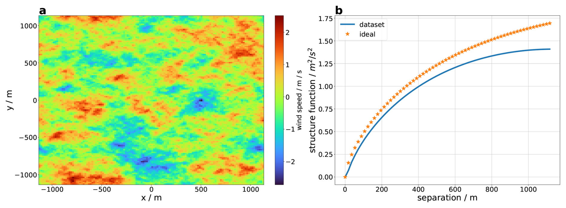
Figure 1 A 2-D wind field example generated by the RPM. (a) A single wind field generated using the RPM. (b) Theoretical structure function in orange stars; dataset's expected structure function in blue.

4 RPM's discretization errors

As an example of the RPM application, consider generating a 2-D wind field representing only the velocity component along the x axis, u_x(s). In this case, Eq. (4) becomes

$$\begin{array}{}\text{(11)}& C_{\text{xx}}\left(\mathit{k}\right)=\sqrt{{\mathrm{\Phi }}_{\text{xx}}\left(\mathit{k}\right)}.\end{array}$$

Consequently, u_x(s) is

$$\begin{array}{}\text{(12)}& u_x\left(\mathit{s}\right)=\text{Re}/\text{Im}\left\{{\mathcal{F}}^{-\mathrm{1}}\left(\mathit{\mu }\left(\mathit{k}\right){\displaystyle \frac{\mathrm{2}\mathit{\pi }}{\sqrt{L_x{L}_y}}}{N}_x{N}_y\sqrt{{\mathrm{\Phi }}_{\text{xx}}\left(\mathit{k}\right)}\right)\right\},\end{array}$$

where L_i is the domain size in the ith direction, N_i is the number of pixels in the ith direction, and μ(k) is a N_x×N_y matrix of complex random variables with zero mean and unit variance. To test the RPM accuracy, a single wind field has been generated implementing Eq. (12) considering a von Kármán (VK) spectrum with a turbulence outer scale of L₀ = 756 m on a square grid of dimensions 3L₀×3L₀. The expected dataset's structure function is computed by setting μ(k)=1 in Eq. (12), while the theoretical structure function is computed using Eq. (9), where, in the case of the velocity component along the x axis in a 2-D domain, the correlation function B(r) is as follows (Batchelor, 1953):

$$\begin{array}{}\text{(13)}& B\left(\mathit{r}\right)={\mathit{\sigma }}^{\mathrm{2}}\left[{\displaystyle \frac{r_x^{\mathrm{2}}}{{\mathit{r}}^{\mathrm{2}}}}f\left(\mathit{r}\right)+{\displaystyle \frac{r_y^{\mathrm{2}}}{{\mathit{r}}^{\mathrm{2}}}}g\left(\mathit{r}\right)\right],\end{array}$$

where σ² is the wind speed variance, and f(r) and g(r) are the longitudinal and lateral correlation functions, respectively. Assuming a VK spectrum, these are as follows (Wilson, 1998):

$$\begin{array}{}\text{(14)}& {\displaystyle }f\left(\mathit{r}\right)={\displaystyle \frac{\mathrm{2}}{\mathrm{\Gamma }(\mathrm{1}/\mathrm{3})}}{\left({\displaystyle \frac{\mathit{r}}{\mathrm{2}{L}_{\mathrm{0}}}}\right)}^{\mathrm{1}/\mathrm{3}}{K}_{\mathrm{1}/\mathrm{3}}\left({\displaystyle \frac{\mathit{r}}{L_{\mathrm{0}}}}\right),\text{(15)}& {\displaystyle }\begin{array}{rl}g\left(\mathit{r}\right)=& {\displaystyle \frac{\mathrm{2}}{\mathrm{\Gamma }(\mathrm{1}/\mathrm{3})}}{\left({\displaystyle \frac{\mathit{r}}{\mathrm{2}{L}_{\mathrm{0}}}}\right)}^{\mathrm{1}/\mathrm{3}}\\ & \times \left[K_{\mathrm{1}/\mathrm{3}}\left({\displaystyle \frac{\mathit{r}}{L_{\mathrm{0}}}}\right)-{\displaystyle \frac{\mathit{r}}{\mathrm{2}{L}_{\mathrm{0}}}}{K}_{\mathrm{2}/\mathrm{3}}\left({\displaystyle \frac{\mathit{r}}{L_{\mathrm{0}}}}\right)\right],\end{array}\end{array}$$

where K_ν is the modified Bessel function of the second kind of order ν. The generated wind field; its structure function; and the expected one, computed substituting Eq. (13) in Eq. (9), are represented in Fig. 1. By analyzing the expected and theoretical structure functions, it is clear that the generated wind field does not properly represent the required statistics, underestimating the spectral power and, thus, the wind speed variance, especially for larger values of the separation vector r.

This error arises due to the fact that the PSD is not a bandwidth-limited function in the desired wavenumber domain; hence, the implementation of the DFT generates a sampling error, as stated in the Nyquist–Shannon sampling theorem (Shannon, 1949). In fact, using the DFT, the wavenumber domain on which the PSD is computed is determined by the grid's spatial resolution, as represented in Fig. 2, where it is clear how the spatial grid acts as a sort of band-pass filter, considering only part of the spectra. A possible way to circumvent the power underestimation at low wavenumbers is to increase the actual spatial grid size while maintaining the same spatial resolution. However, this approach depends on the considered PSD and on the grid shape, and so it has to be optimized for each specific case. Moreover, for some applications (e.g., when employing this approach in a Monte Carlo setup), this is not possible due to computational reasons because of the large memory size that the grid would end up having. Consequently, other methods that reduce this error calculation-wise have been developed.

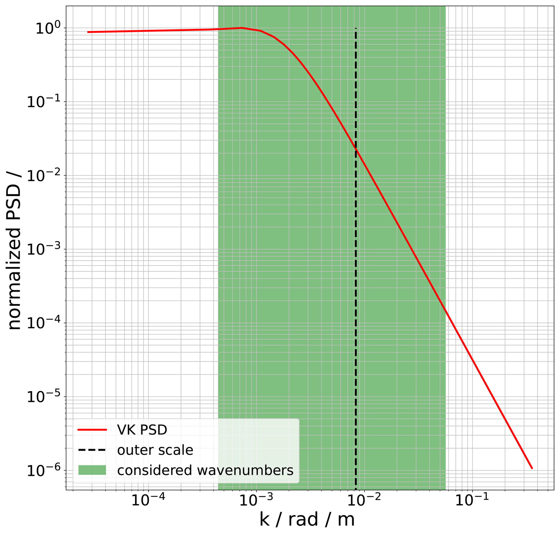
Figure 2 The spatial grid acting as a band-pass filter. The green rectangle represents the considered wavenumbers for a spatial domain of the order of 3 times the outer scale. In this case, it is expected to underestimate the power both at the high and at the low wavenumbers. The red line represents the VK spectrum, and the dashed black line represents the turbulence outer scale – also referred to as the integral length scale.

For example, the sub-harmonic method (Sedmak, 1998) decreases the inaccuracies in the low-wavenumber region, replacing the single sample at the origin in the wavenumber domain with nine (or even more) sub-samples. These samples represent an equivalent length that is 3 times higher than the length of a simple grid, allowing us to sample the PSD at lower wavenumbers and enhancing the dataset accuracy at high spatial scales.

Another corrective method, proposed in Xiang (2014), implements a modal decomposition of the correlation function. The correlation function is pre-processed, extracting the piston and tilt components, and a mask is applied. The tilt and piston components are then used to compute a tilt screen that is added to the dataset generated using Eq. (12). However, the drawback of such methods is that they are not of a general nature (i.e., they cannot be applied for all kinds of PSDs); consequently it is necessary to compute different weighting parameters for each considered spatial domain. Moreover, these methods can be applied only on square grids.

5 The CB-RPM: generating the wind field from the correlation tensor

The here-proposed CB-RPM has been developed with the aim of eliminating the bandpass effect of the DFT that arises while using the RPM. To solve this problem, the relation between the correlation function and the PSD (i.e., the two quantities being a Fourier pair, as expressed in Eq. 8) can be used. Indeed, by calculating the PSD used in the dataset's synthesis from the theoretical correlation function, computed on the spatial domain s, the sampling error is eliminated. This solution and how to generate a stochastic dataset from it were first investigated theoretically in Cramer and Leadbetter (1967), from which several methods, mainly used in the field of geostatistics, have followed. Some of these methods (Dietrich and Newsam, 1993; Wood and Chan, 1994) rely on embedding a Toeplitz correlation matrix, computed from the correlation function, in a circulant matrix, from which the desired dataset is synthesized by means of eigenvalue decomposition. However, these methods do not allow us to compute the dataset directly from the wind correlation function. Another proposed method, the FIM (Pardo-Iguzquiza and Chica-Olmo, 1993), is very similar to the here-proposed CB-RPM, computing the PSD from the correlation function. However, in the case of the CB-RPM, no arrangements of the Fourier coefficients in the wavenumber domain are needed before computing the dataset. The CB-RPM can be described by the following steps:

1. Compute the correlation function. In the case of a homogeneous turbulent wind field, the correlation tensor is (Batchelor, 1953)

   $$\begin{array}{}\text{(16)}& B_{\text{pq}}\left(\mathit{r}\right)={\mathit{\sigma }}^{\mathrm{2}}\left[{\displaystyle \frac{r_p{r}_q}{{\mathit{r}}^{\mathrm{2}}}}f\left(\mathit{r}\right)+\left({\mathit{\delta }}_{\text{pq}}-{\displaystyle \frac{r_p{r}_q}{{\mathit{r}}^{\mathrm{2}}}}\right)g\left(\mathit{r}\right)\right],\end{array}$$

   where δ_pq is the Dirac delta function, and f(r) and g(r) are the longitudinal and lateral correlation functions. In the case of a 2-D domain and assuming a VK spectrum, they are defined by Eqs. (14) and (15), respectively.

2. Compute the PSD. The corresponding PSD, Φ_CB-RPM(k), is the Fourier transform of the theoretical correlation function, B_pq(r).

   $$\begin{array}{}\text{(17)}& {\mathrm{\Phi }}_{\text{CB-RPM}}\left(\mathit{k}\right)=\mathcal{F}\left(B_{\text{pq}}\right(\mathit{r}\left)\right)\end{array}$$

   In the above, the obtained Φ_CB-RPM is not the theoretical PSD, but it is the discrete Fourier pair of the theoretical correlation function B_pq(r) in the desired spatial domain. Note that Φ_CB-RPM(k) is not a tensor, as in Mann (1998), because it is the Fourier transform of the tensor component B_pq and not of the whole tensor. B_pq already takes into account the longitudinal and lateral correlation, as described in Eq. (16).

3. Synthesize the dataset. The random dataset u_p(s) can be generated by taking the real or imaginary component of the DIFT of the square root of Φ_CB-RPM(k) multiplied with a set of complex Gaussian random variables with zero mean and unity variance μ(k).

   $$\begin{array}{}\text{(18)}& u_p\left(\mathit{s}\right)=\text{Re}/\text{Im}\left\{{\mathcal{F}}^{-\mathrm{1}}\left(\mathit{\mu }\left(\mathit{k}\right)\sqrt{{\mathrm{\Phi }}_{\text{CB-RPM}}\left(\mathit{k}\right)N}\right)\right\}\end{array}$$

   The novelty of the CB-RPM with respect to the FIM lies in this last step. Indeed, the CB-RPM does not need to divide the wavenumber domain into different regions where the amplitude spectrum's coefficients (i.e., the square root of the PSD) are computed as it is needed in the FIM, but the PSD Φ_CB-RPM is used directly in that computation, resulting in a faster computation having one step less than the FIM.

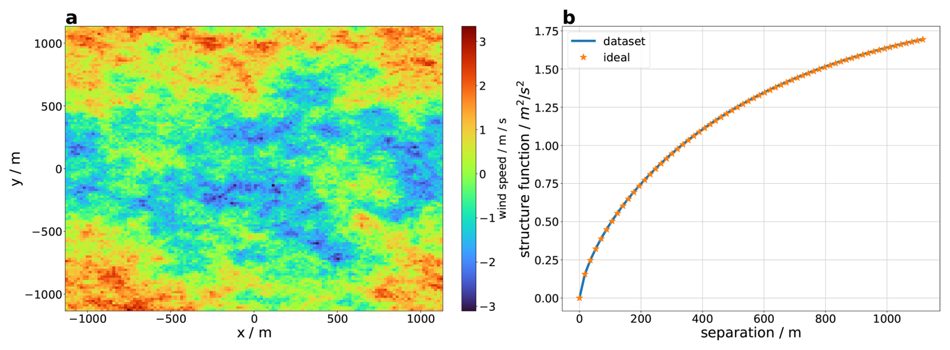
Figure 3 A 2-D wind field example generated with the CB-RPM. (a) A single wind field generated using the CB-RPM. (b) Theoretical structure function in orange stars; dataset's expected structure function in blue.

6 Validating the CB-RPM in different spatial domains

As an example of the CB-RPM application, a single component wind field has been generated on a 2-D domain using the same parameters as in Sect. 4. In the case of a 2-D domain and considering the velocity along the x axis, the generated wind field u_x(s) is

$$\begin{array}{}\text{(19)}& u_x\left(\mathit{s}\right)=\text{Re}/\text{Im}\left\{{\mathcal{F}}^{-\mathrm{1}}\left(\mathit{\mu }\left(\mathit{k}\right)\sqrt{\mathcal{F}\left(B_{\text{xx}}\left(\mathit{r}\right)\right)N_x{N}_y}\right)\right\},\end{array}$$

where B_xx is the VK correlation function, computed using Eq. (13). The synthesized wind field u_x, its structure function, and the expected one are represented in Fig. 3. The expected structure function matches the theoretical one exactly, demonstrating that the synthesized dataset u_x(s) respects the required statistics.

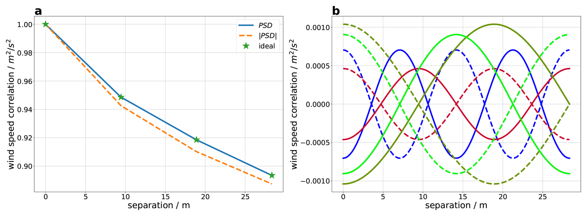
Figure 4 Negative DFT coefficient contribution. (a) The theoretical correlation function is in green stars, the correlation function computed assuming negative values in the PSD is in blue, and the correlation function computed using the absolute value of the PSD is in dashed orange. (b) The different colors represent the contribution to the correlation function computation of four different DFT coefficients. The contribution of the negative coefficients is represented with continuous lines, and the contribution of the same coefficients but with a positive value is represented with dashed lines. The difference between the sum of the two sets of lines gives the expected error if the absolute value of the PSD is used.

In order to verify the actual generality of the method (i.e., it can be used without the need for any parameter optimization in any spatial domain), the expected structure function has been calculated for a wide range of spatial grid dimensions, starting from 0.01L₀ up to 10L₀. Similarly to the function Φ_FFT in Xiang (2014), for very small spatial domains with respect to the turbulence outer-scale L₀, the obtained PSD, Φ_CB-RPM(k), yields negative values. This is theoretically incorrect because the PSD is defined as a positive function. The cause of the occurrence of these negative values is due to the implementation of the DFT on very small spatial domains. In fact, for very small spatial domains, the correlation function becomes almost flat, requiring some of the DFT coefficients to be phase-shifted by a factor π (i.e., having negative-amplitude values) in order to synthesize the desired shape in the spatial domain. Considering the extreme case in which the correlation function is a circular flat surface, its Fourier transform would be a jinc function (Goodman, 1996). Thus, the appearance of negative values in Φ_CB-RPM(k) is expected for very small spatial domains. One simple solution would be to take the absolute value of Φ_CB-RPM(k); however, this would lead to an error in the dataset's correlation function as shown in Fig. 4, where a single component wind field is generated on a 2-D, 8 × 8 grid of length 0.1L₀ and L₀ = 756 m.

To tackle the issue regarding negative PSD values, it is possible to consider only the positive part of the PSD and to reduce the error by pre-compensating for the correlation function, as proposed in Xiang (2014). The proposed pre-compensation consists of subtracting to the theoretical correlation function, defined in Eq. (13), with the weighted error being generated by neglecting the negative-amplitude wavenumbers of the PSD:

$$\begin{array}{}\text{(20)}& B_W\left(\mathit{r}\right)=B_{\text{xx}}\left(\mathit{r}\right)-W\left(\mathit{r}\right){\mathrm{\Delta }}_{\mathrm{\Phi }}\left(\mathit{r}\right),\end{array}$$

where the error Δ_Φ(r) is computed as

$$\begin{array}{}\text{(21)}& {\mathrm{\Delta }}_{\mathrm{\Phi }}\left(\mathit{r}\right)=B_{\text{xx}}\left(\mathit{r}\right)-\mathcal{F}\left[H\left({\mathrm{\Phi }}_{\text{CB-RPM}}\right(\mathit{k}\left)\right){\mathrm{\Phi }}_{\text{CB-RPM}}\left(\mathit{k}\right)\right],\end{array}$$

where H() is the Heaviside function, and the weight W(r) has the shape of an elliptic super Gaussian window.

$$\begin{array}{}\text{(22)}& W\left(\mathit{r}\right)=A{\mathrm{e}}^{-C\left[{\left(\frac{r_x}{E}\right)}^g+{\left(\frac{r_y}{F}\right)}^g\right]},\end{array}$$

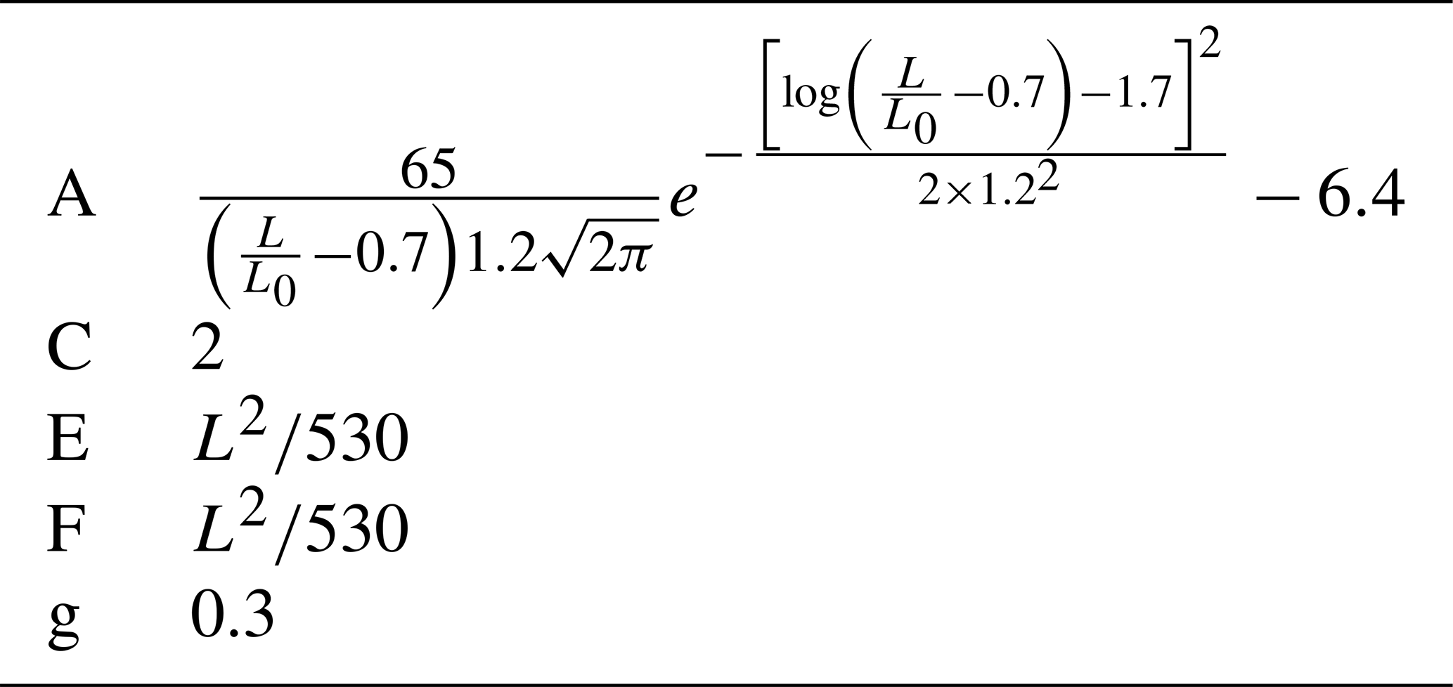
In the above, g is the super Gaussian function exponent, and A, C, E, and F are parameters that can be optimized depending on the considered PSD and the required dataset's accuracy. In this case, Eq. (19) becomes the following:

$$\begin{array}{}\text{(23)}& u_p\left(\mathit{s}\right)=\text{Re}\left\{{\mathcal{F}}^{-\mathrm{1}}\left(\mathit{\mu }\left(\mathit{k}\right)\sqrt{\mathcal{F}\left(B_W\left(\mathit{r}\right)\right)N_x{N}_y}\right)\right\}.\end{array}$$

The parameters proposed for a square 64 × 64 grid with dimensions of L × L and a VK spectrum are reported in Table 1.

Table 1 WCB-RPM compensation parameters.

Using the weighted CB-RPM (WCB-RPM) with these parameters, the obtained error is 3 to 5 times lower than the one obtained with the CB-RPM for very small spatial domains with respect to the turbulence outer-scale L₀.

7 Comparing the RPM and the CB-RPM

The errors of both methods have been compared on a wide range of spatial grid dimensions, starting from 0.01L₀ up to 10L₀. For each grid, the method error Δ_i has been computed as follows:

$$\begin{array}{}\text{(24)}& {\mathrm{\Delta }}_i=\text{max}\left(\mathit{\epsilon }\right({\mathit{r}}_i\left)\right),\end{array}$$

where ε(r_i) is computed using Eq. (10) for the separation vector r_i, and the dataset's structure function D(r_i) is computed using Eq. (9), where the dataset's correlation function is computed as

$$\begin{array}{}\text{(25)}& B\left({\mathit{r}}_i\right)=\stackrel{\mathrm{‾}}{u_x\left(\mathit{s}\right)u_x(\mathit{s}+{\mathit{r}}_i{)}^{\ast }}.\end{array}$$

It has been decided that we should consider the maximum error value for each spatial domain for conservative reasons. The comparison between the two methods is represented in Fig. 5, where it is clear how the CB-RPM outperformed the RPM by at least 1 order of magnitude, confirming that the method is a reliable solution in the synthesis of Gaussian processes without the need for any parameter optimization. For spatial domains greater than 2.5L₀, a region which is relevant for the simulation of aircraft turbulence encounters (Kiehn et al., 2022), the CB-RPM can be declared to be exact in principle (Wood and Chan, 1994), meaning that the method error is limited by the computer arithmetic inaccuracies. The novelty of the CB-RPM with respect to the RPM lies in its performance, especially for spatial domains greater than 2.5L₀, as represented in Fig. 5. If a greater accuracy is needed in low spatial domains, the WCB-RPM can be used by implementing Eq. (23) (dashed green line in Fig. 5) and by reducing the error by up to 2 orders of magnitudes with respect to the RPM. It should be noted that the WCB-RPM parameters presented here can be further optimized. However, this is left to possible later applications as the authors' objective is to generate wind fields for spatial domains around 20L₀, where the CB-RPM performs excellently. Initially it was thought to compare the synthesized datasets with their PSDs, but, to avoid the biases generated by computing the dataset's PSD using Eq. (7) and the underestimation of the dataset's power due to windowing (Thomson, 1982), it was considered to be more appropriate to compare the synthesized datasets' correlation functions, computed using Eq. (25). For the Wiener–Khinchin theorem, the datasets' correlation functions are the Fourier transform of the PSDs. Thus, in the case where the errors of the datasets' correlation functions with respect to the theoretical ones are low, this also applies to the errors of the datasets' PSDs.

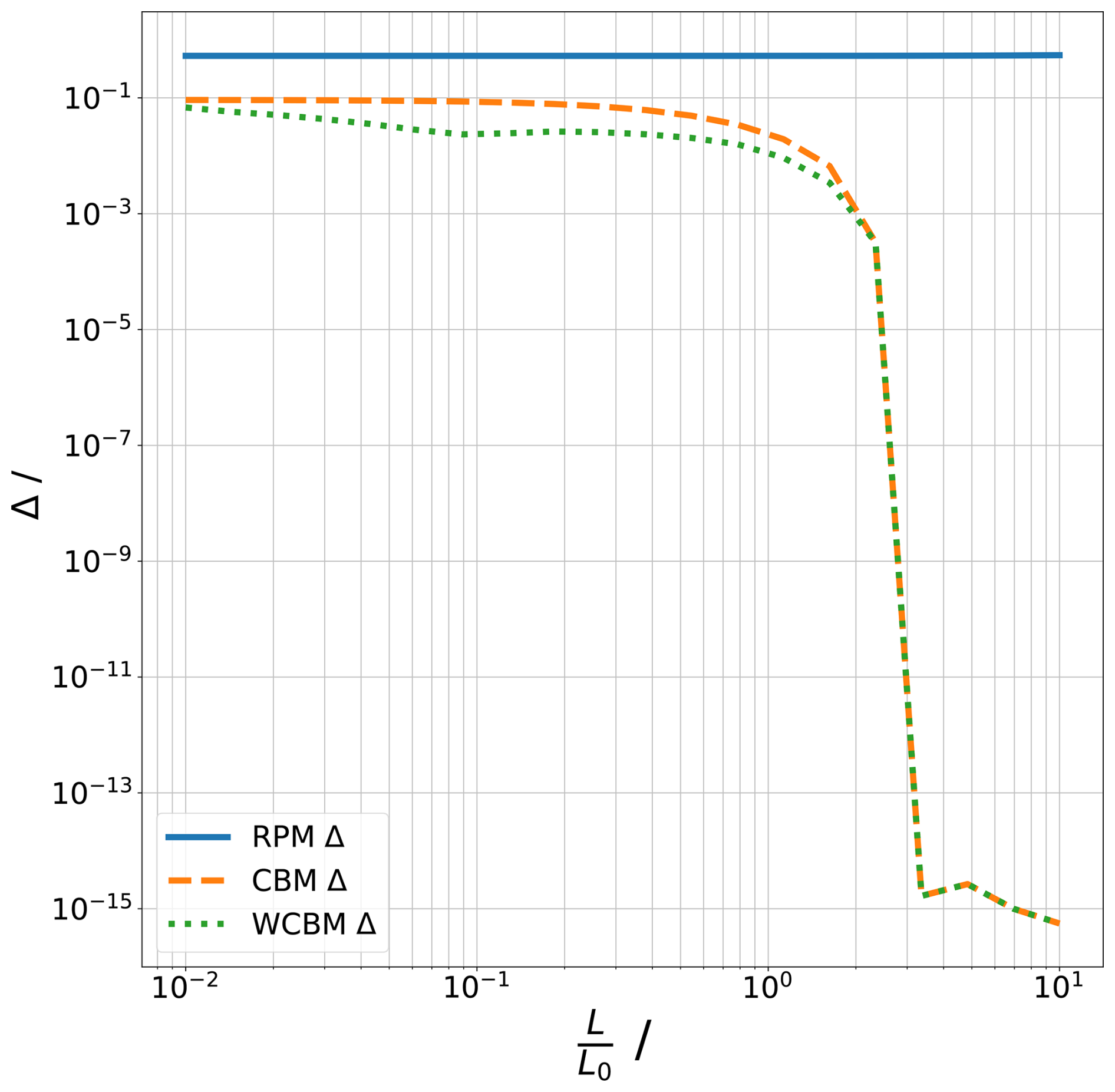
Figure 5 Method comparison. RPM errors are in blue, CB-RPM errors are in dashed orange, and WCB-RPM errors are in dotted green. The x axis indicates the ratio between the considered spatial domain and the turbulence outer scale.

8 Conclusions

In this publication a new method for synthesizing Gaussian and stationary phenomena has been presented. This new method allows the generation of a dataset with an error of at least 1 order of magnitude lower than the commonly used RPM. For spatial domains greater than 2.5L₀, the CB-RPM can be declared to be exact in principle. This refers to the computational errors and not to how close the synthesized wind field is to reality. Indeed, the CB-RPM was developed to decrease the errors of the synthesized wind field with respect to the theoretical structure function and not real data. In this paper the assumption of homogeneous and isotropic turbulence has been made; however, especially for turbulence near the surface, this assumption is no longer valid (Panofsky and Dutton, 1984). In this case, the wind field correlation function can be refined by computing it from real data, measured employing anemometers or five-hole probes, from high-resolution large-eddy simulation (LES) results (Yoshimura et al., 2023) or by considering a non-stationary wind and following the method presented in Wilson (1997). The authors are working to expand the use of CB-RPM to these cases as well. Furthermore, being a general method, it can be used to synthesize any phenomenon considered to be Gaussian and stationary (e.g., index of refraction fluctuations, temperature fluctuations, homogeneous and isotropic turbulence) only by knowing the phenomenon's structure or correlation function. These functions can be obtained by means of analytical solutions (e.g., from the Kolmogorov cascade theory, Kolmogorov, 1941) or from real measurement data, allowing us to synthesize phenomena for which no analytical solutions exist (e.g., clear-air turbulence (CAT) events; Knox, 1997). A further advantage of the method is that it allows, in a relatively simple way, the representation of anisotropies in the phenomenon of interest: these can be directly added to the theoretical correlation from which the PSD is computed (Pardo-Iguzquiza and Chica-Olmo, 1993). The method is also valid for non-symmetrical spatial domains, an interesting result that can be applied to highly customized wind speed dataset generation. The authors are working on adding other types of spectra (e.g., the Kaimal spectrum, Kaimal et al., 1972, or the Mann uniform shear turbulence model, Mann, 1994) to the CB-RPM. A further development would be the use of the CB-RPM for the synthesis of wind fields starting from any wind dataset provided by the user. This would allow further investigation of anisotropies found during aircraft measurements (Nowak et al., 2025) while still assuming homogeneous turbulence. Moreover, it is foreseen that there will be the possibility of implementing the addition of non-Gaussian features to the synthesized wind field following the method proposed in Friedrich et al. (2022). Finally, a routine to automatically compute the weighting function W(r) starting from the error Δ_Φ(r) is being developed. This would allow us to achieve better performance in small spatial domains with respect to the turbulence outer-scale L₀.