Gaussian process surrogate modeling for efficient controller tuning and fatigue load prediction of the helix wake-mixing method

Wind farms experience reduced power production and elevated structural loading due to wake interactions. Wake-mixing control techniques, which dynamically excite upstream turbine wakes to accelerate recovery, have demonstrated promising improvements in downstream power production but at the expense of increased fatigue loading. Identifying the optimal control settings and quantifying the resulting load implications remain challenging because these methods require high-fidelity simulations that capture both the dynamic actuation and the resulting turbulence. Moreover, existing load surrogate models do not incorporate wake-mixing control, largely because conventional engineering wake models are unable to reproduce periodic wake excitation. This study presents two complementary advances to improve the design of wake-mixing strategies using a limited number of large eddy simulations (LES) and Gaussian process (GP) regression. First, we develop an efficient simulation-driven framework to identify optimal frequency and amplitude parameters for wake-mixing control, yielding a clear optimal power gain of 7.5 % near a Strouhal number of 0.25 and pitch amplitudes of around 4° for a two-turbine array. Second, we present a surrogate model capable of predicting fatigue loads for wake-mixing control. Using LES-derived rotor-plane inflow fields for aeroelastic simulations, we construct a load database that encompasses various combinations of wake overlap, turbine spacing, and wind farm control settings. The result is a load surrogate model based on GP regression trained on sector-averaged inflow quantities that accurately predicts damage equivalent loads, including the effect of increased excitation in the wake. This model enables the joint evaluation of power gains and load penalties at the wind farm level, supporting a more informed design of wake-mixing control strategies. Applying the load surrogate model to a two-turbine case study demonstrates the trade-off between additional power gain and increased structural loading of both turbines with the helix method.

1 Introduction

Wind farms that are densely spaced suffer from power production losses and increased structural loads as wind turbines are, at times, subject to turbulent wakes (Meyers et al., 2022). These wakes arise as turbines extract energy from the incoming flow, leaving a zone characterized by lower wind speeds and higher turbulence. The field of wind farm flow control (WFFC) attempts to minimize the negative implications of the wake effect by altering the wake to improve power efficiency and/or reduce fatigue loading. Wind farm flow control methods can be categorized into three groups. First, static induction control (SIC) tries to reduce the velocity deficit and turbulence intensity in the wake by altering one of the steady-state operating setpoints (generally the pitch angle or tip-speed ratio) of a turbine (Kanev et al., 2018). Effectively, this method more evenly redistributes the power output and loading over multiple turbines, without significantly improving the overall wind farm performance (van der Hoek et al., 2019). Second, wake steering control adds an additional control variable to the turbine in the form of a yaw misalignment. This misalignment of the turbine with the dominant wind direction introduces a lateral component of the thrust force acting on the incoming flow, resulting in a wake that is steered away from downstream turbines (Fleming et al., 2014; Gebraad et al., 2016). While a yaw misalignment reduces the energy production of a wind turbine, downstream turbines benefit from higher inflow velocities and can improve the combined power output of the wind farm. Last, for wake-mixing control, upstream turbines are dynamically actuated to excite the wake and trigger wake recovery mechanisms at an earlier stage. This is generally achieved by feeding a periodic reference signal for collective pitch control (Munters and Meyers, 2018b), individual pitch control (Frederik et al., 2020a), or yaw control (Munters and Meyers, 2018a).

Unlike WFFC methods that adjust a static control setpoint such as SIC or wake steering, the effectiveness of wake-mixing techniques also relies on the amplitude and frequency of excitation. Where steady-state wind farm simulation tools like FLORIS (NREL, 2024) or PyWake (Pedersen et al., 2023) are generally used to optimize yaw angles and induction factors, the optimal frequency and amplitude for wake-mixing methods are obtained through high-fidelity models such as large eddy simulations (LES). Initial studies on periodic dynamic induction control indicated an optimal frequency for a Strouhal number of St=0.25 (Munters and Meyers, 2018b). The dimensionless Strouhal number is expressed as $\mathit{St}=f_{\mathrm{e}}\cdot D/U_{\mathrm{\infty }}$, with excitation frequency f_e, rotor diameter D, and inflow velocity U_∞. Successive simulation studies (Frederik et al., 2020a; Muscari et al., 2022) and experimental campaigns (Frederik et al., 2020b; van der Hoek et al., 2024) on wake-mixing methods observed slightly different optima in the range of St=0.2–0.4. These previous studies indicate that the optimal frequency can depend on multiple aspects, such as the ambient conditions (e.g., wind speed, turbulence intensity), the turbine model, and the simulation environment. When adding the actuation amplitude as a control variable, one can imagine that determining the optimal control settings requires a large number of computationally expensive simulations.

Compared to other WFFC strategies, wake-mixing techniques such as the helix method do not rely on precisely redirecting the wake away from the downstream rotor, a task that is particularly sensitive to wind direction uncertainty. Wake mixing has instead been shown to increase power performance by enhancing wake recovery directly (Frederik et al., 2020a; Taschner et al., 2023). Under low wind veer conditions, the helix method has even been found to outperform wake steering in terms of power production (Frederik et al., 2025), and recent studies also showed the helix to be more robust to wind direction variations than wake steering in the case of full turbine alignment (Taschner et al., 2024; Baricchio et al., 2026). This performance benefit, however, comes at the expense of increased fatigue loading (Frederik et al., 2020a).

van Vondelen et al. (2023) showed increased fatigue loads using aeroelastic simulations for a turbine applying the helix method for all components considered. Furthermore, the increase in fatigue loads was shown to be more sensitive to increasing pitch amplitudes than to actuation frequency. Similar studies by Frederik and van Wingerden (2022) and Frederik et al. (2025) combining LES and aeroelastic simulations also focused on the effect of wake-mixing methods on fatigue loads of a downstream turbine. These studies showed increased loading due to the additional turbulence introduced into the wake by the periodic excitation. However, the simulations were limited to a select number of cases with fixed distance and alignment of the two turbines, and a single pitch amplitude. A more comprehensive study on the effects of wake-mixing techniques on downstream turbine loads, considering different spacing and alignment cases, is currently missing from the literature.

To assess the fatigue loading to which wind turbines are subjected under different conditions (i.e., atmospheric, operational, wake effects), load surrogate models are a more efficient alternative to running expensive simulations for each case. These models are generally based on large databases of aeroelastic simulations and can predict fatigue loads based on some inflow or layout variables. Although these models require a large number of simulations for training, once trained, they enable efficient prediction and offer significant flexibility. Dimitrov et al. (2018) used various site-specific ambient conditions (e.g., wind speed, turbulence intensity, shear exponent, wind veer) to construct a load database and used these conditions as inputs to compare multiple surrogate models for predicting fatigue loads. Accurate load predictions were obtained with polynomial chaos expansion (PCE) and Kriging methods. However, their database did not consider turbines operating in wake conditions. To account for wake-induced loads, a follow-up study included additional information, consisting of turbine spacing, wake incidence angle, and the number of upstream turbines, in the surrogate models (Dimitrov, 2019). A similar approach from Mendez Reyes et al. (2019) used wake parameters such as depth, width, and lateral spacing between the wake and the rotor to build a multidimensional lookup table (LUT) based on aeroelastic simulations. Furthermore, this LUT included the effect of WFFC methods, such as wake steering and SIC, on fatigue loads. The load surrogate models discussed so far required information on the location of a turbine with respect to the wake. More recently, several studies presented layout-agnostic load surrogate models. Shaler et al. (2022) removed the location dependency by solely considering several inflow statistics along different lines spanning the rotor plane to train a variety of surrogate models. Alternatively, the rotor wind field can be reconstructed using proper orthogonal decomposition (POD), which provides a reduced-order model of the flow through the superposition of a selected number of modes (Liew et al., 2024). A further simplification was proposed by Guilloré et al. (2024), who discretized the inflow (velocity and turbulence intensity) into sectors. An artificial neural network (ANN) trained with these sector-averaged inflow quantities provided accurate fatigue load estimates using only four sectors.

While some of the studies discussed in the previous paragraph evaluated the effect of WFFC on fatigue loads, the implementation of wake-mixing techniques was not included. This is primarily related to the methods for generating the load databases, which rely on the combination of aeroelastic simulations to compute the turbine loads, synthetic turbulence to generate the inflow, and engineering wake models to generate the wake inflow for downstream turbines. For example, Shaler et al. (2022) and Guilloré et al. (2024) used FAST.Farm (Jonkman and Shaler, 2021) to obtain inputs for their load surrogate models. As wake-mixing techniques depend on the dynamic actuation of the wake, such a simulation framework is not suitable for capturing the effects of wake-mixing control on fatigue loading. The increased complexity of wake-mixing control, resulting from its dynamic actuation and reliance on high-fidelity simulations, together with its associated increase in fatigue loading, is precisely why an efficient, load-aware modeling approach is needed to evaluate whether this trade-off is worthwhile in a given scenario.

This paper adds to the state-of-the-art in wake-mixing control in several ways. We present a data-driven framework based on Gaussian process (GP) regression that models the performance of the helix method, accounting for both energy yield and fatigue loads. More specifically, this framework is used to obtain the following contributions.

• Efficiently determining the optimal settings for wake-mixing techniques (i.e., the helix method) using a limited number of LES and GP regression

• A surrogate model for predicting WFFC fatigue loads, modeled as a GP with sector-averaged inflow quantities as proposed by Guilloré et al. (2024). Inflow for the aeroelastic simulations is generated from LES to capture the periodic nature of the wake

• Evaluating WFFC performance in terms of energy yield and fatigue loads with the helix method on a two-turbine array under different operational conditions in terms of the helix pitch amplitude and array alignment

The remainder of this paper is structured as follows. Section 2 describes the methodology, including the simulation tools and settings, and the GP model framework. Section 3 presents the framework for efficient wake-mixing controller tuning and its application in a two-turbine array. In Sect. 4, we validate the load surrogate model and test it in a case study with two turbines. Finally, we conclude the paper with a summary and recommendations in Sect. 5.

2 Methodology

Both the wake-mixing tuning framework and the load surrogate model rely on LES. This section covers the simulation environment that was used to acquire a realistic representation of wind turbine loading and wake behavior. Next, the WFFC methods that we consider for the load surrogate model are summarized. Finally, a general description of Gaussian processes is provided.

2.1 Simulation environment

The high-fidelity simulations that were run for this paper were performed on the Adaptive Mesh Refinement for Wind (AMR-Wind) simulator (Kuhn et al., 2025). AMR-Wind is part of the ExaWind modeling and simulation environment (Sharma et al., 2024), built on top of the AmRex library (Zhang et al., 2019). The simulator solves the three-dimensional incompressible Navier–Stokes equations in a spatially filtered resolved-scale formulation and employs the subgrid-scale one-equation turbulence model (Moeng, 1984) for smaller eddy dynamics.

2.1.1 Precursor simulations

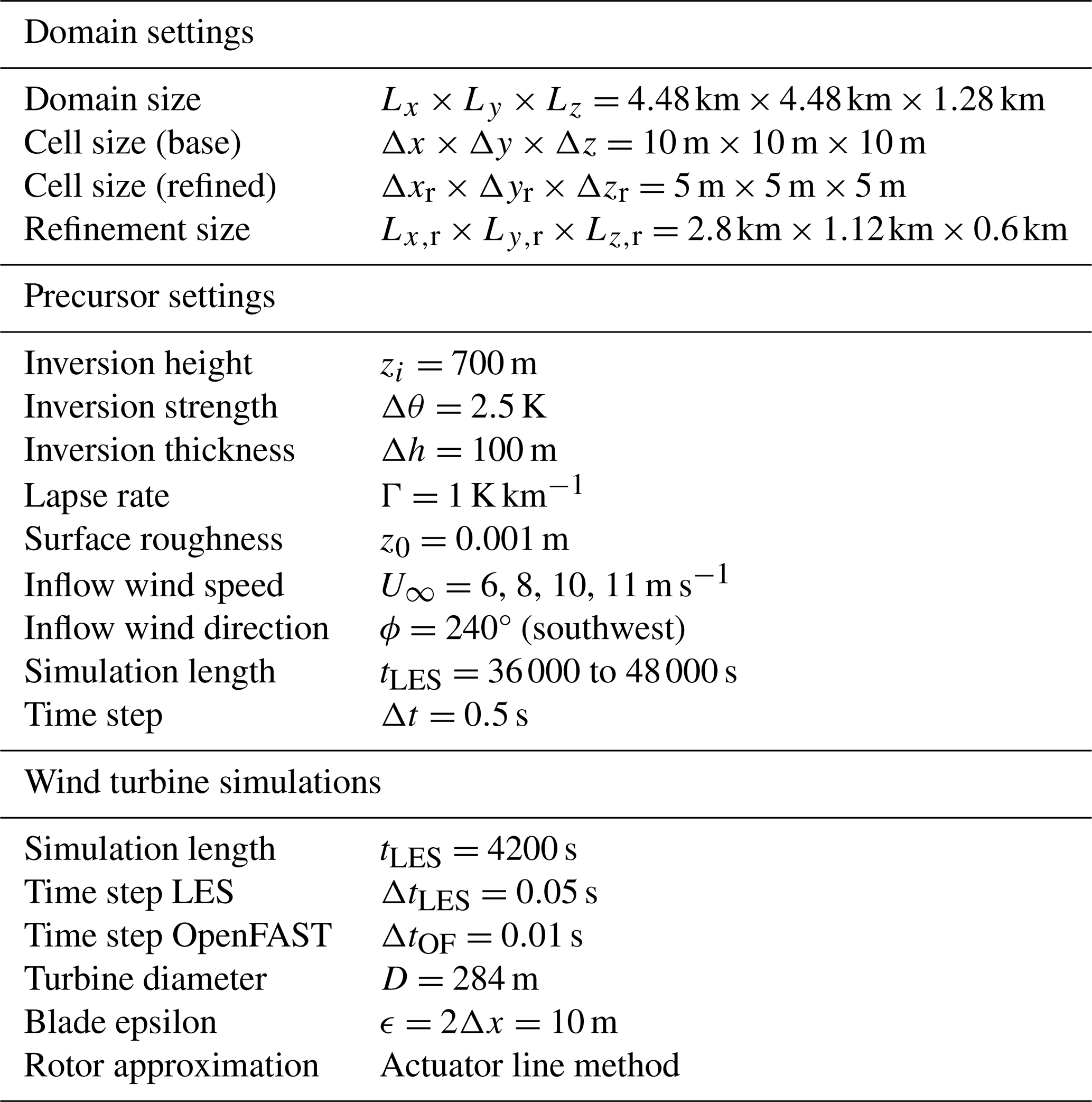
Several precursor simulations of a conventionally neutral boundary layer (CNBL) were run to generate the turbulent inflow for the wind turbine simulations. We used a simulation domain of $L_x\times L_y\times L_z=\mathrm{4.48}$ km × 4.48 km × 1.28 km, with 10 m equidistant cells. Coriolis forces were included, with the latitude of the domain set to ϕ_lat=52.6° to match conditions on the Dutch North Sea. For the CNBL, a potential temperature profile with an inversion height of z_i=700 m was prescribed. The ground temperature was set to θ₀=288.15 K, and a capping inversion strength of Δθ=2.5 K was used over a thickness of Δh=100 m, followed by a lapse rate of Γ=1 K km⁻¹. The surface roughness was set to z₀=0.001 m, which resulted in a turbulence intensity that varied between 3 %–6 % over the rotor area. The resulting conditions are similar to those encountered on the North Sea (Türk and Emeis, 2010). Precursor simulations were generated for wind speeds in the range of 6–11 m s⁻¹, as this range coincides with the below-rated operating region of the turbine where WFFC is most effective. The wind direction was set to 240° (southwest), with periodic boundary conditions on the x and y boundaries. The precursors were simulated between 36 000 and 48 000 s, depending on inflow velocity, to allow sufficient time for turbulence to develop and reach a quasi-steady state. After this period, the boundary conditions at the inflow boundaries are sampled for the next 70 min to be used later on for the turbine simulations. An overview of all the precursor simulation settings is provided in Table 1. An example of one of these precursor profiles is given in Fig. 1, showing the prescribed temperature profile, the velocity magnitude U_∞, turbulence intensity (TI), and wind direction (veer) ϕ as a function of height.

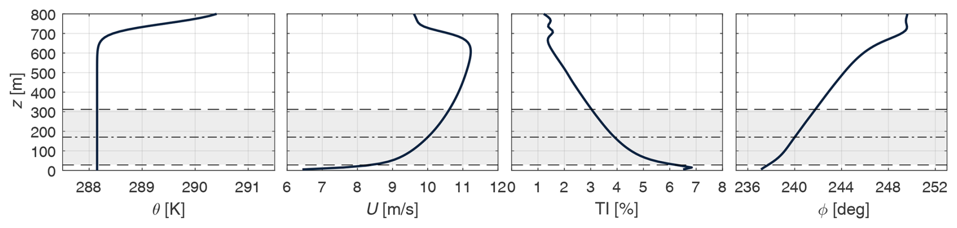
Figure 1 Average profiles of temperature (θ), wind speed (U), turbulence intensity (I), and wind veer (ϕ) over height (z) for one of the precursor simulations in AMR-Wind. The dash-dotted line indicates the turbine hub height, while the shaded areas indicate the height spanned by the wind turbine rotor.

2.1.2 Wind turbine simulations

When simulating one or multiple turbines, we used the coupling between AMR-Wind and the OpenFAST aeroelastic simulator (National Renewable Energy Laboratory, 2024) to model the response of the wind turbine. The turbine model is that of the IEA 22 MW reference wind turbine (Zahle et al., 2024). The turbine has a rotor diameter of D=284 m and a hub height of z_H=170 m, with a rated wind speed of U_rat=11 m s⁻¹. Within the LES, the aerodynamic forces of the turbine are modeled using the AeroDyn (v15.03) module of OpenFAST, which are subsequently applied to the incoming flow using the actuator line method (ALM). The ALM model uses 59 actuator points per blade, corresponding to the number of airfoil files for the IEA 22MW turbine used by AeroDyn.

The simulation domain around the turbines was refined once to obtain cells of Δx_r=5 m. The refinement region starts two diameters (2 D) in front of the first turbine, spanning a width of 4 D, a height of 2.1 D, and a length of 10 D. A schematic of the simulation domain is provided in Fig. 2. The resulting resolution in terms of rotor diameter is $D/\mathrm{\Delta }x\approx \mathrm{56}$, which is sufficient for ALM (Martínez-Tossas et al., 2015). The blade force projection from the ALM onto the incoming flow was done with a Gaussian kernel width of $\mathit{ϵ}=\mathrm{2}\mathrm{\Delta }x=\mathrm{10}$ m to prevent numerical instabilities (Martínez et al., 2012). The LES ran with a constant time step of Δt_LES=0.05 s, ensuring that the blades do not skip any grid cells in subsequent time steps. The time step of the OpenFAST simulation was set to Δt_OF=0.01 s. Each simulation was run for a total of 4200 s, of which the first 600 s was used to let the wake develop and only the last 3600 s were considered for analysis. An overview of the simulation settings is provided in Table 1.

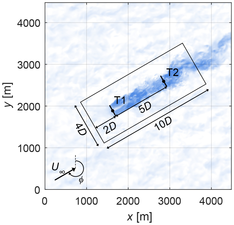
Figure 2 Schematic of a simulation setup in AMR-Wind. The simulation domain has dimensions 15.7 $D\times \mathrm{15.7}D\times \mathrm{4.5}D$. A single mesh refinement (4 $D\times \mathrm{10}D\times \mathrm{2.1}D$) is indicated by the rectangle enclosing the turbines. The two turbines are separated by a distance of 5 D. The flow is coming from the southwest direction of the simulation domain.

Table 1 Settings for the simulations performed with AMR-Wind.

2.2 Wind farm flow control methods

Within the simulations, the turbines were controlled using the reference open-source controller (ROSCO) toolbox for wind turbine applications (Abbas et al., 2022). In the baseline control case, the turbines were operated to maximize their own power production. The WFFC methods that are considered for the load surrogate model include wake steering (Fleming et al., 2014; Gebraad et al., 2016) and the helix method (Frederik et al., 2020a; Korb et al., 2023). Although we only consider these methods, the load surrogate model can easily be extended to include other strategies, such as static induction control. Implementing wake steering in the simulations is straightforward and consists of adding a constant offset to the turbine yaw angle.

With the helix control strategy, individual blade pitch control is used to exert time-varying blade moments on the incoming flow. These moments are designed in such a way that, when transformed from a rotating to a non-rotating reference frame (Bir, 2008), slowly varying yaw and tilt moments are applied to the flow. These moments create the characteristic helical shape of the wake. An example of the blade pitch signals is given in Fig. 3. Each of the sinusoidal reference signals is offset by a phase of 120°. Increasing the amplitude (A_β) of the pitch signals results in stronger yaw and tilt moments, and hence, in a more pronounced helix shape. The excitation frequency (f_e) at which the yaw and tilt moments move across the rotor plane is generally expressed using the dimensionless Strouhal number (St):

$$\begin{array}{}\text{(1)}& f_{\mathrm{e}}={\displaystyle \frac{\mathit{St}\cdot U_{\mathrm{\infty }}}{D}},\end{array}$$

with U_∞ indicating the freestream inflow velocity. The pitch actuation frequency (f_β) is then defined as

$$\begin{array}{}\text{(2)}& f_{\mathit{\beta }}=f_{\mathrm{r}}\pm f_{\mathrm{e}},\end{array}$$

with f_r denoting the rotational frequency of the rotor. Adding the excitation frequency (f_e) to the rotational frequency (f_r) results in a counterclockwise-rotating helix wake, while subtracting the excitation frequency yields a clockwise-rotating helix wake. For the simulations, we used the built-in functionality of the Active Wake Control module in ROSCO to implement the helix approach, which requires settings for the amplitude, excitation frequency, and direction. The resulting pitch reference signal for each of the blades (β_i) at time t is then defined as

$$\begin{array}{}\text{(3)}& {\mathit{\beta }}_i\left(t\right)={\mathit{\beta }}_{*}+A_{\mathit{\beta }}\sin \left(\mathrm{2}\mathit{\pi }(f_{\mathrm{r}}+f_{\mathrm{e}})t+{\mathit{\psi }}_{\mathrm{0},i}\right),\end{array}$$

where β_* is the optimal collective pitch angle and ψ_0,i represents the azimuth angle of blade i at t=0. Higher pitch amplitudes result in larger wake deflections, but they are accompanied by higher power losses and increased structural loading (Taschner et al., 2023).

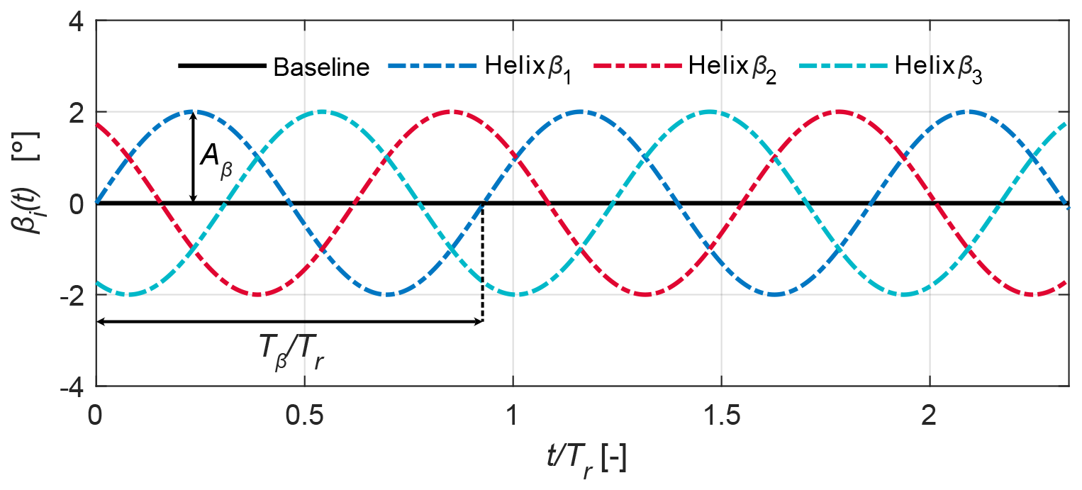
Figure 3 Example of the pitch reference signals (β_i) for the counterclockwise helix implementation. The amplitude of the signals is indicated by A_β. The period of the pitch actuation is given by $T_{\mathit{\beta }}=f_{\mathit{\beta }}^{-\mathrm{1}}$, normalized by the duration of one rotor rotation period $T_{\mathrm{r}}=f_{\mathrm{r}}^{-\mathrm{1}}$.

2.3 Gaussian process surrogate model

The LES described in the previous sections are very computationally expensive. Each wind turbine simulation requires several days of simulation time on a high-performance computing (HPC) cluster. Therefore, simulating a full sweep of all control parameters for the helix method becomes very time-consuming, especially when multiple ambient conditions need to be considered. When one also wants to evaluate the effects of WFFC methods on fatigue loads under different alignment and spacing conditions, simulating this becomes unfeasible. To make this problem tractable, this paper uses surrogate models trained on a limited number of LES.

Before introducing the mathematical formulation, we briefly summarize the role of GP regression (Rasmussen and Williams, 2006) in this framework. A GP allows us to construct a computationally cheap (compared to LES) surrogate model of a relationship that would otherwise require many expensive LES or aeroelastic simulations to characterize, such as turbine power as a function of wake-mixing control settings, or fatigue loads as a function of inflow and control conditions. This is achieved in three steps. First, a limited set of simulations is used to generate training data, consisting of pairs of known inputs (e.g., control settings or inflow conditions) and their corresponding outputs (e.g., power or fatigue load). Second, the GP model is trained on this dataset by tuning a set of hyperparameters that determine how strongly the modeled function is correlated between different input locations. Third, the trained model is used to predict the output along with its associated uncertainty for new input conditions, without requiring additional simulations. In this paper, this framework is applied twice: first, to model the power output of a two-turbine array as a function of the helix frequency and amplitude (Sect. 3) and, second, to predict fatigue loads as a function of inflow and control conditions (Sect. 4). These two applications place different demands on the GP model. For the load surrogate model, the training data are generated in advance from a fixed database of simulations, and the aim is to obtain an accurate representation of the fatigue loads across the full range of inflow and control conditions, since predictions may later be required for arbitrary combinations of these conditions. In the controller tuning framework, the GP serves a dual aim, which is to obtain a model that shows where, and to what extent, the helix method is effective across the frequency–amplitude domain, and to use this model to make informed decisions on which settings to simulate next.

When considering a GP, we assume that the output data, collected in a one-dimensional vector y, belong to a multivariate Gaussian distribution

$$\begin{array}{}\text{(4)}& :\left[\begin{array}{c}\mathit{y}\\ {\mathit{y}}^{\mathbf{*}}\end{array}\right]\sim \mathcal{N}\left(\mathbf{0},\left[\begin{array}{cc}\mathbf{K}\left(\mathbf{x},\mathbf{x}\right)+{\mathit{\sigma }}_n^{\mathrm{2}}\mathbf{I}& \mathbf{K}\left(\mathbf{x},{\mathbf{x}}^{*}\right)\\ \mathbf{K}\left({\mathbf{x}}^{*},\mathbf{x}\right)& \mathbf{K}\left({\mathbf{x}}^{*},{\mathbf{x}}^{*}\right)\end{array}\right]\right).\end{array}$$

The distribution of the output depends on one or multiple inputs collected in a matrix x. The vector y^* refers to the inferred function value for possible test inputs x^*. The covariance matrix K can be computed from a wide range of kernel functions and depends on the type of function one would like to model. Two popular options are the squared exponential and Matérn functions (Rasmussen and Williams, 2006), which will both be used in this work. Each Kernel function is equipped with a set of hyperparameters that control the output scaling, correlation, and level of smoothness. An additional hyperparameter is given in the form of σ_n, which represents the noise or uncertainty in the output data. In this work, the hyperparameters are obtained by maximizing the log marginal likelihood. After determining the hyperparameters, we compute the posterior distribution of the model, resulting in the mean (μ^*) and variance (Σ^*) for the test locations (x^*) using the following set of equations:

$$\begin{array}{}\text{(5)}& {\displaystyle }{\mathit{\mu }}^{*}=\mathbf{K}\left({\mathbf{x}}^{*},\mathbf{x}\right){\left(\mathbf{K}\left(\mathbf{x},\mathbf{x}\right)+{\mathit{\sigma }}_n^{\mathrm{2}}\mathbf{I}\right)}^{-\mathrm{1}}\mathit{y},\text{(6)}& {\displaystyle }{\mathbf{\Sigma }}^{*}=\mathbf{K}\left({\mathbf{x}}^{*},{\mathbf{x}}^{*}\right)-\mathbf{K}\left({\mathbf{x}}^{*},\mathbf{x}\right){\left(\mathbf{K}\left(\mathbf{x},\mathbf{x}\right)+{\mathit{\sigma }}_n^{\mathrm{2}}\mathbf{I}\right)}^{-\mathrm{1}}\mathbf{K}\left(\mathbf{x},{\mathbf{x}}^{*}\right).\end{array}$$

The content of the test input matrix (x^*) depends on the application. When we want to determine the optimal control settings for the helix method, this matrix consists of different combinations of actuation frequency and pitch amplitude. In the case of evaluating fatigue loads, this matrix consists of the inflow conditions, as well as some control inputs. Both cases will be considered in more detail in the subsequent sections.

2.4 Load surrogate database

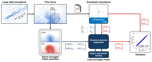
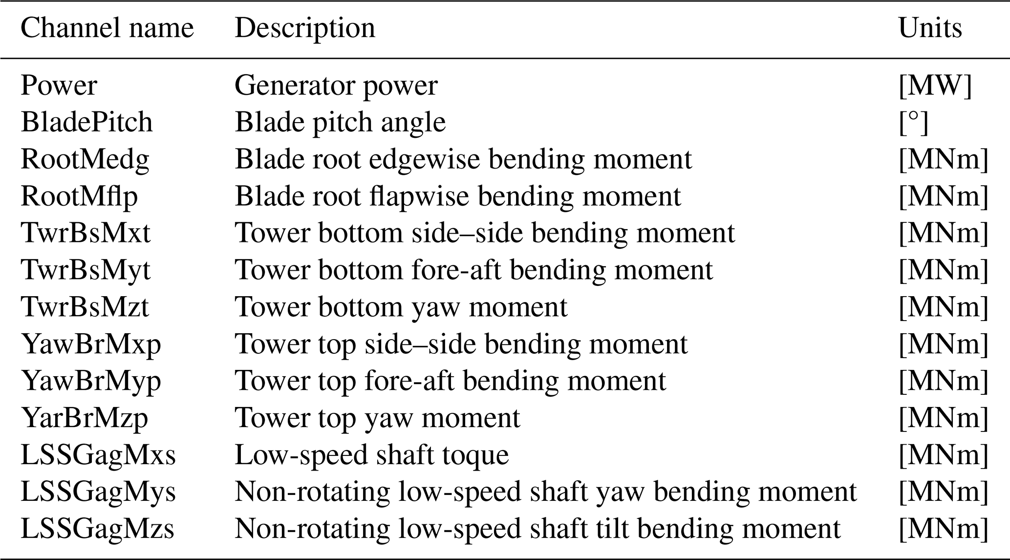
This section describes how the load surrogate model is constructed. The overall workflow to obtain the surrogate model is illustrated in Fig. 4. In short, cross-stream velocity flow slices are extracted from the LES at different downstream distances and wake displacements, representing a range of wake conditions. These flow slices are then used as time-varying inflow for standalone aeroelastic simulations in OpenFAST, from which structural load time series are obtained for the turbine components listed in Table 2, accompanied by a brief description. The resulting load time series are converted into damage equivalent loads (DELs), while the corresponding flow slices are reduced to four sector-averaged velocity and turbulence intensity values. Finally, these sector-averaged inflow quantities, together with the relevant control settings (i.e., helix pitch amplitude A_β and yaw misalignment γ), are used as inputs to train a separate GP model for each load channel, allowing fatigue loads to be predicted directly from inflow and control conditions without additional aeroelastic simulations. The remainder of this section details each of these steps.

Cross-stream flow slices were collected at a 1 s interval from the wake of a single turbine at distances between 3D and 8D, as well as a slice of the undisturbed precursor inflow. Subsequently, these time series were cut into blocks of 660 s to mimic the effect of different turbulence seeds of the inflow conditions. Next, the flow slices were projected on a rectangular grid of 340 m (≈1.20 D) width by 330 m (≈ 1.16 D) height, with grid spacing of 10 m (≈ 0.04 D), and exported to a .wnd file compatible with OpenFAST. To simulate different levels of wake overlap, a displacement parameter Δy was introduced to move the grid laterally over the cross-stream flow slices. In this way, the aeroelastic simulations covered all wake conditions from full overlap (Δy=0 m) to no wake overlap (at close turbine spacing with baseline control and for $\mathrm{\Delta }y=\pm \mathrm{390}$ m ≈1.37 D). It should be noted that the 1 Hz sampling frequency of the extracted flow slices could limit the high-frequency inflow-driven load content, and some structural excitation present in a full LES-driven simulation may not be captured by standalone OpenFAST simulations at higher frequencies. However, sampling the inflow at a frequency similar to that of the LES was not feasible from a data storage perspective.

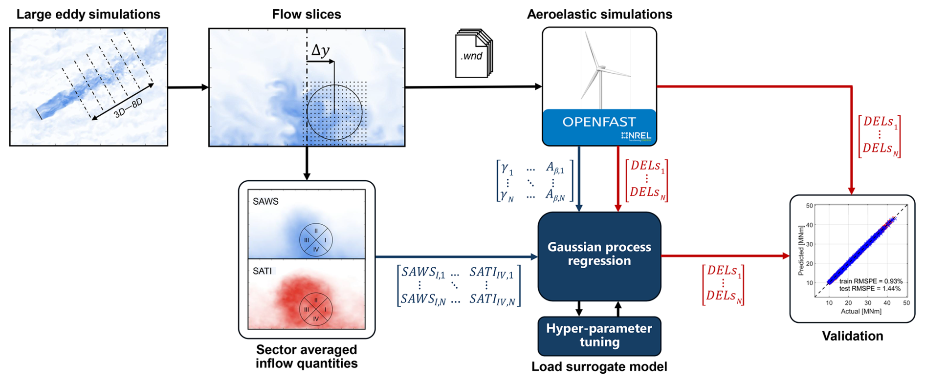
Figure 4 Schematic of the framework for training and validating the load surrogate model. Flow slices are extracted from large eddy simulations and used as inflow for aeroelastic simulations. The resulting load time series are converted into damage equivalent loads and sent to a GP model along with some turbine control inputs and the sector-averaged inflow quantities. The GP model can subsequently predict fatigue loads based on a set of input conditions.

Table 2 List of considered wind turbine channels obtained from the OpenFAST simulations.

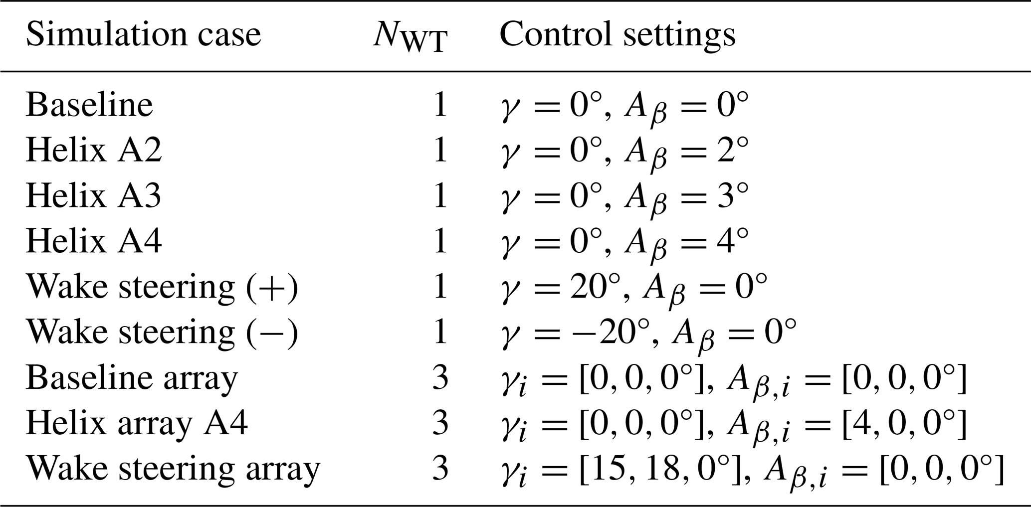
In the LES cases used to obtain the flow slices, we employed different control strategies, including greedy control, wake steering, and the helix method. Furthermore, several simulations with three turbines, each separated by a distance of 4.5 D, were conducted to include the effect of accumulated turbulence in the wake. From these simulations, flow slices from the wake of the second and third turbines were collected. For now, we assume that these inflow conditions are representative of larger wind farm configurations, but this requires additional validation at a later stage. An overview of all the control strategies that were simulated is provided in Table 3. These control cases were simulated with the precursor wind speeds specified in Table 1, resulting in a total of approximately 30 LES runs for the load surrogate database. The standalone OpenFAST simulations for the loads database also include the turbine using different control strategies to assess the impact on loads. For wake steering, the turbine was yawed with $\mathit{\gamma }=\left\{-\mathrm{30}:\mathrm{10}:\mathrm{30}\mathit{°}\right\}$, and for the helix method, the pitch amplitude was varied between $A_{\mathit{\beta }}=\left\{\mathrm{1.0}:\mathrm{1.0}:\mathrm{4.0}\mathit{°}\right\}$.

In terms of computational cost, each LES run requires between 1 and 2 d of runtime on an HPC cluster. Extracting and post-processing the flow slices, and subsequently running the standalone aeroelastic simulations for the range of wake displacements and control settings described above, is comparably expensive and adds a further several days of computation time. Once the resulting loads database is available, however, training the GP surrogate model is considerably cheaper. Optimizing the hyperparameters for a single load channel takes around 10–20 min. In the current framework, the computational bottleneck lies almost entirely in generating the training data rather than in training the surrogate model itself.

Table 3 LES cases that were run for each precursor wind speed to generate the inflow for the loads database. For each case, the number of turbines N_WT and the control setpoints (γ, A_β) are provided.

The entries for the load surrogate database were obtained after post-processing the time series of the inflow planes and the load channels. The first set of inputs sent to the load surrogate model are the sector-averaged inflow quantities, as proposed by Guilloré et al. (2024). In this case, the inflow consisting of streamwise velocity and turbulence intensity is averaged over four sectors spanning the rotor plane. For the sector-averaged wind speed (SAWS) U_SA(s), the wind speed value for each sector s is determined in the following way:

$$\begin{array}{}\text{(7)}& U_{\mathrm{SA}}\left(s\right)=\underset{\mathit{\psi }=\left(\frac{(s-\mathrm{1})\cdot \mathit{\pi }}{\mathrm{2}}-\frac{\mathit{\pi }}{\mathrm{4}}\right)}{\overset{\mathit{\psi }=\left(\frac{s\cdot \mathit{\pi }}{\mathrm{2}}-\frac{\mathit{\pi }}{\mathrm{4}}\right)}{\int }}\underset{r=\mathrm{0}}{\overset{r=R}{\int }}r\cdot \overline{u}(\mathit{\psi },r)\mathrm{d}r\mathrm{d}\mathit{\psi }.\end{array}$$

In the previous equation, the local time-averaged streamwise wind speed $\overline{u}$ from the LES flow planes is integrated over the radial distance r and the azimuth angle ψ, where the latter has been discretized into four sectors. The same equation is used to determine the sector-averaged turbulence intensity (SATI), where turbulence intensity is defined as

$$\begin{array}{}\text{(8)}& \text{TI}={\displaystyle \frac{\sqrt{\frac{\mathrm{1}}{\mathrm{3}}\left(\stackrel{\mathrm{‾}}{u^{\prime }{u}^{\prime }}+\stackrel{\mathrm{‾}}{v^{\prime }{v}^{\prime }}+\stackrel{\mathrm{‾}}{w^{\prime }{w}^{\prime }}\right)}}{U_{\mathrm{\infty }}}}.\end{array}$$

Here, u^′, v^′, and w^′ indicate the instantaneous velocity deviations from the average for the streamwise, transverse, and vertical velocity components, respectively. Furthermore, $\stackrel{\mathrm{‾}}{u^{\prime }{u}^{\prime }}$ denotes the time average of the velocity fluctuations squared. Note that the freestream wind speed velocity U_∞ is selected to normalize the root mean square of the average velocity fluctuations instead of the local average wind speed. In this case, the TI sectors provided as input to the load surrogate model are higher for turbines operating in a helix wake. Hence, the surrogate model can predict the additional fatigue loading resulting from the helix wake. This was done to distinguish between the wake of a turbine operated with greedy control and the helix method, as the latter generally causes higher velocity fluctuations.

To assess the effect of control strategies and wake conditions on the fatigue loads, time series from the load channels are converted into 1 Hz DELs using the following equation:

$$\begin{array}{}\text{(9)}& L_{\mathrm{eq}\mathrm{1}\mathrm{Hz}}={\left({\displaystyle \frac{{\sum }_{i=\mathrm{1}}^{N_{\mathrm{bins}}}{n}_i\cdot L_i^m}{N_{\mathrm{cycles}}}}\right)}^{\frac{\mathrm{1}}{m}}.\end{array}$$

The number of load cycles n_i and load amplitude L_i for a bin i are obtained from a standard rainflow counting algorithm for N_bins=200. The Wöhler slope coefficient is set to m=10 for the composite blades and m=4 for the steel tower components. Finally, N_cycles refers to the number of 1 Hz cycles in the 10 min time series, as per convention, equaling a value of 600. The DEL can be interpreted as the load amplitude that does a similar amount of damage at a 1 Hz interval as the load time series.

The use of wake-mixing techniques can also have a significant impact on the blade pitch bearings due to the combination of continuous movement and alternating load cycles. One method to express the loads that the pitch bearings experience is using the pitch bearing damage equivalent load (PBDEL) (van Vondelen et al., 2024). The PBDEL (L_PB) is determined using the following equation:

$$\begin{array}{}\text{(10)}& \begin{array}{rl}& L_{\mathrm{PB}}\left(\mathit{\chi }\right)\\ & ={\left({\displaystyle \frac{{\sum }_{k=\mathrm{1}}^{N_{\mathrm{steps}}}\mathit{\delta }\mathit{\beta }\left(k\right)\cdot max{\left(\cos \left(\mathit{\chi }\right)\cdot M_{\text{flp}}\left(k\right)+\sin \left(\mathit{\chi }\right)\cdot M_{\text{edg}}\left(k\right),\mathrm{0}\right)}^m}{N_{\mathrm{ref}}}}\right)}^{\frac{\mathrm{1}}{m}}.\end{array}\end{array}$$

The PBDELs are determined for the full range of radial positions of the bearings with 10° increments, i.e.,  $\mathit{\chi }=\mathit{\{}\mathrm{0}:\mathrm{10}:\mathrm{360}\mathit{°}\mathit{\}}$. The degree of pitch travel is denoted by δβ(k) for a time step k. The blade root flapwise and edgewise bending moments are given by M_flp and M_edg, respectively. N_ref indicates the reference degree of pitch travel during a 10 min interval. In this study, we set N_ref=600°, which matches the distance a blade travels when applying the helix with an amplitude of A_β=2.0° and with St=0.25 at a wind speed of U_∞=10 m s⁻¹. For the pitch bearings, a Wöhler coefficient of m=3 is used (Zahle et al., 2024). For the load surrogate model, we always consider the radial position that experiences the highest load.

3 Efficient tuning of wake-mixing control settings

This section presents the framework for tuning wake-mixing control settings, demonstrated for a two-turbine array simulated with AMR-Wind as described in Sect. 2 at a wind speed of U_∞=8 m s⁻¹. The GP regression framework serves two complementary purposes in this context. First, it acts as a sequential experimental design tool. At each iteration, the GP mean and uncertainty are used to guide the selection of the next LES, focusing computational effort on the most informative regions of the parameter space. This allows optimal settings to be identified from a smaller number of simulations (approximately 20 in the present study) than the 50 or more runs a representative grid search over frequency and amplitude would require. Each LES yields six 10 min average samples, corresponding to approximately 120 training points in total. Given the modest dataset size, fitting the GP hyperparameters at each iteration takes on the order of seconds. New simulation settings were selected manually based on visual inspection of the GP mean and uncertainty at each iteration. The frequency range was first explored broadly to characterize the overall shape of the power ratio function, after which subsequent simulations focused on the narrower range identified as most promising.

Formal optimization algorithms, such as Bayesian optimization, provide a systematic way to balance exploration and exploitation through an acquisition function and would be a suitable choice for this problem. However, we consider this most valuable either when the selection of new points must itself be fast and automated or when the design space cannot be visualized directly, i.e., when more than two inputs are considered. In this study, each LES run required several days of computation time, so the time needed to manually inspect the GP model and select a new simulation setting is negligible in comparison, and the one- or two-dimensional design space considered here could be visualized and interpreted directly. We therefore consider the manual selection approach adopted here to be an appropriate choice for the present study, while acknowledging that an automated, acquisition-based approach such as Bayesian optimization would become increasingly relevant as additional inputs (e.g., ambient conditions) are added to the model and the design space can no longer be easily visualized.

The second purpose of the GP framework is to provide a smooth function of the power ratio surface across the full frequency–amplitude domain. This allows one to efficiently evaluate, for any given control setting, whether deploying the helix is expected to yield a net power gain, how large that gain is likely to be, and the expected variation in power gain due to the turbulent nature of the inflow. Although demonstrated here for low-turbulence conditions, the framework is applicable to other wake-mixing strategies and can be expanded to include different atmospheric conditions.

3.1 Wind turbine measurements

The simulation data required for the data-driven modeling framework are extracted as time series from the OpenFAST output files. An example of such a simulation output is given in Fig. 5, showing the generator power of the upstream (T1) and downstream (T2) turbines for the baseline case and the helix method. The time series show a slight decrease in power for T1, and a significant increase in power for T2, when the helix method is used. The 1 h measurement domain is then divided into multiple 10 min periods, and the power is averaged over time, as shown on the right-hand side of Fig. 5. Note that the relative power of the helix method over the baseline can vary depending on the 10 min time interval, due to the turbulent eddies that hit the turbines. This indicates the importance of sufficient simulation time and the use of multiple data points for a single helix case.

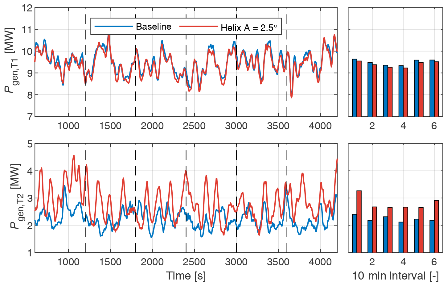
Figure 5 Power generated by the upstream (T1) and downstream (T2) turbines over time (left) and the 10 min average power comparing baseline control to the helix method (right). The vertical dashed lines indicate the 10 min intervals used for averaging.

The time-averaged power data are subsequently used to compute the power ratio ($\frac{P_{\mathrm{WFFC}}}{P_{\mathrm{BL}}}$) of the helix method over baseline control. All the power ratio measurements are then collected and scaled to a zero mean and unity standard deviation dataset y. Similarly, we collect the training locations, consisting of the helix amplitude and frequency, in a matrix x and scale it before feeding it to the GP model as training data. For the GP to effectively identify the contribution of both turbines to the total power of the array, the model is split into two parts with their own set of hyperparameters. Hence, we obtain a GP model that estimates the power loss of T1 (μ_T1, σ_T1) due to the helix actuation, and a GP model that estimates the power gain or loss for turbine T2 (μ_T2, σ_T2) due to the affected wake recovery. A useful property of Gaussian processes is that the sum of two Gaussian processes is also a Gaussian process. Therefore, we can model the mean and variance of the total power gain as follows:

$$\begin{array}{}\text{(11)}& {\displaystyle }{\mathit{\mu }}_{\mathrm{array}}& {\displaystyle }={\mathit{\mu }}_{\mathrm{T}\mathrm{1}}+{\mathit{\mu }}_{\mathrm{T}\mathrm{2}},\text{(12)}& {\displaystyle }{\mathit{\sigma }}_{\mathrm{array}}^{\mathrm{2}}& {\displaystyle }={\mathit{\sigma }}_{\mathrm{T}\mathrm{1}}^{\mathrm{2}}+{\mathit{\sigma }}_{\mathrm{T}\mathrm{2}}^{\mathrm{2}},\end{array}$$

where μ_array is the mean power gain of the two turbines, and ${\mathit{\sigma }}_{\mathrm{array}}^{\mathrm{2}}$ is the variance of the estimated mean power gain.

3.2 Controller tuning results

After extracting power data from the simulations and post-processing them, we can iteratively determine the optimal settings for the helix method for the current ambient conditions. We used a Matérn covariance function (Rasmussen and Williams, 2006) with a smoothness parameter of $\mathit{\nu }=\mathrm{3}/\mathrm{2}$ to get a smooth but flexible model. The GP modeling framework presented in the previous section will now be used to model the power increase in the counterclockwise (CCW) helix implementation. For the sake of demonstration, we first focus on a single input GP model where the Strouhal number is the free variable, and the pitch amplitude is fixed at a value of A_β=2.5°. Using only one input also allows for easier initialization of the model, when the quantity of data is still small. Figure 6 shows the total power gain as a function of the Strouhal number. For each of the subplots, the hyperparameters are first optimized, and the mean power ratio and variance are inferred for a range of other frequencies. Based on the inferred power ratio, a new frequency is selected and subsequently applied in a new LES run, after which the process is repeated.

The model is initialized (see Fig. 6a) using 10 min average data samples from three separate simulations that employed the helix method at different frequencies. For a Strouhal number just above St=0, we see a power ratio below 100 %, indicating a loss of power due to the actuation of the helix method. However, this ratio increases as the Strouhal number rises to values of St=0.2. For the next two simulations (Fig. 6b, c), we focus on exploring the power ratio function by selecting Strouhal numbers of 0.5 and 1.0, respectively. Based on previous studies (Frederik et al., 2020a), we do not expect the optimal frequency to lie within this range, but we are interested in determining the shape of the function and reducing the uncertainty. After updating the GP with these simulation results, the model predicts the highest power ratios to be obtained in the range of St=0.2–0.4. After the latest iteration (Fig. 6f), we notice that the GP estimates show little variation in this frequency range. The power increase for the considered pitch amplitude seems to settle at approximately 4.3 %. The measurement samples also indicate that where the helix method is effective, large variations in the power ratio occur.

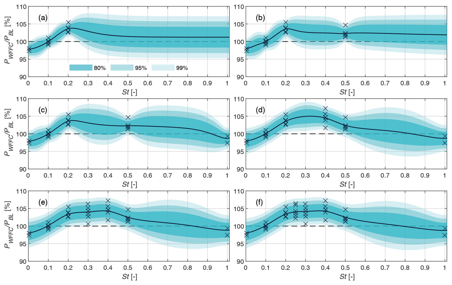
Figure 6 Power ratio of the helix method over baseline operation ($\frac{P_{\mathrm{WFFC}}}{P_{\mathrm{BL}}}$) for the two-turbine array. Samples from the LES used to train the model are denoted by the × marks. Each sample corresponds to a 10 min average taken from the 1 h LES time series. The solid black line indicates the estimated power ratio of the different GP models, and the shaded areas show the uncertainty bounds of the estimated mean power. The subplots from (a)–(f) show different iterations of the GP model after additional data have been acquired.

The next step in the modeling framework is to expand the GP model to include pitch amplitude. This requires only a small alteration to the GP model, consisting of adding an additional input (A_β) and a corresponding input lengthscale (hyperparameter). The model is then trained using all prior data. The same approach for selecting the control settings for the LES runs is adopted as in the previous example, focusing first on exploration, followed by maximizing the power gain. The final versions of the GP models are presented in Fig. 7 as contour maps of the power ratio as a function of frequency and pitch amplitude. From the GP model of turbine T1 shown in Fig. 7a, we see a clear decrease in power for lower frequencies and increasing pitch amplitudes. For the second turbine (Fig. 7b), the power ratio keeps rising for increasing pitch amplitudes. When combining the models of both turbines, we obtain the contour map in Fig. 7c for the total power ratio, indicating a clear optimum. The optimum indicates that for pitch amplitudes above 4°, the additional power loss (with respect to the optimal settings) of the actuated turbine (T1) cannot be compensated for by the increased power of the downstream turbine (T2). The optimal power ratio of 7.5 % was achieved with an amplitude of A_β=4° and a frequency of St=0.25. While the optimal identified frequency agrees well with previous studies (Munters and Meyers, 2018b; Frederik et al., 2020a), Taschner et al. (2023) showed an increasing power trend for even higher pitch amplitudes. However, their simulations were performed with a different turbine model and for a different wind speed.

Figure 7 also shows the two-dimensional estimates of the GP models with uncertainty bounds for the optimal frequency and amplitude. The model for T1 (Fig. 7a) can estimate the power loss with high certainty, with the only uncertainty arising from the lack of samples at higher frequencies. Power losses of up to 5 % are visible for increasing amplitudes at the optimal frequency. The models for T2 (Fig. 7b) and the overall power (Fig. 7c) look very similar to each other, with higher uncertainty in the estimates. Interestingly, the range of optimal frequencies narrows as the pitch amplitude increases. When operating the helix with pitch amplitudes up to 2.5°, this could offer some additional flexibility on the selected frequency. In this case, the optimal frequency is determined not only by the maximum power gain but also by the minimum fatigue loading.

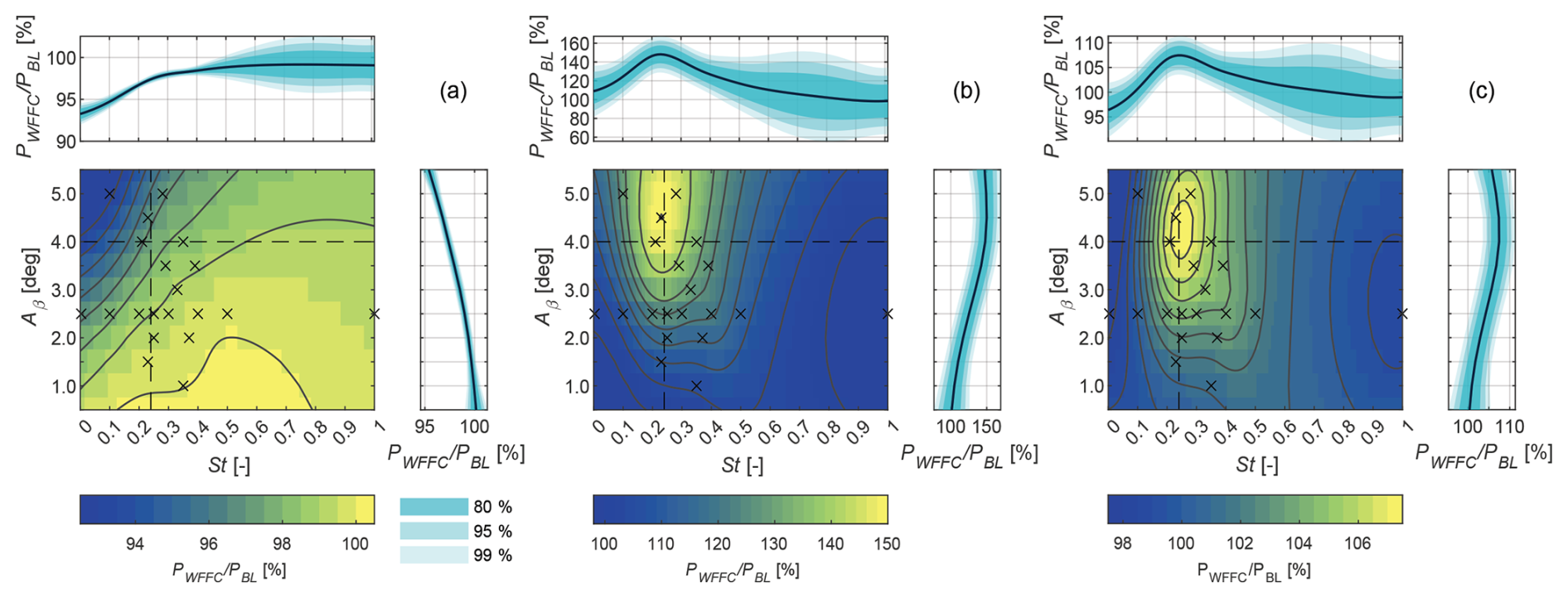
Figure 7 Power ratio of the helix method over baseline operation ($\frac{P_{\mathrm{WFFC}}}{P_{\mathrm{BL}}}$). The figure shows the estimated power ratio of turbine T1 (a), turbine T2 (b), and the combined power of the turbine array (c). Samples from the LES used to train the model are denoted by the × marks. The contour maps indicate the estimated mean power ratio of the different GP models. The dashed lines denote the optimal frequency and amplitude for the total power gain. The accompanying estimates and uncertainty bounds are shown above and to the right of the contour maps.

Modeling the performance of wake-mixing techniques has thus far been limited to the CCW helix method. In Fig. 8, the model is modified to include clockwise (CW) simulations of the helix method. For this model, we assume the shape of the GP model for the CW helix is similar to the CCW version. The model is therefore extended by mirroring the frequency axis around the rotational frequency f_r. For the CW excitation of the helix, the blade pitching frequency will be below the rotational frequency of the turbine, as seen in Eq. (2). Figure 8 shows that the CW helix method achieves similar power gains to CCW for pitch amplitudes up to 2°. For higher pitch amplitudes, the gain remains fairly constant, which means that the power loss of the actuated turbine is not overcompensated for by the power gain of the downstream turbine.

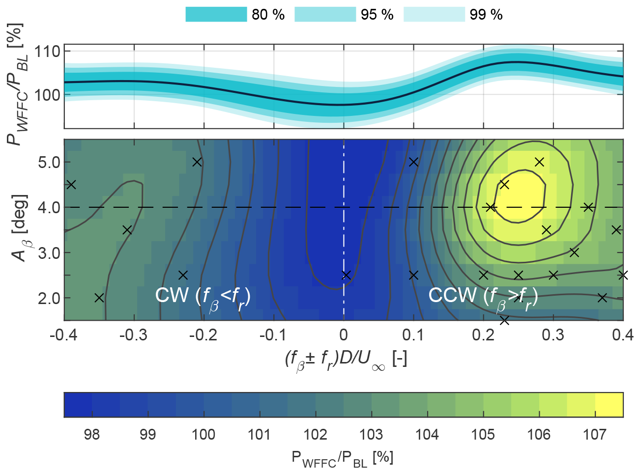
Figure 8 Power ratio of the helix method over baseline operation. The figure shows the estimated combined power of the turbine array, comparing the CW (<0) and CCW (>0) helix implementations. Samples from the LES used to train the model are denoted by the × marks. The dashed black line denotes the optimal amplitude for the total power gain. The accompanying estimates and uncertainty bounds are shown above the contour map.

The tuning framework has so far been demonstrated for a single free-stream wind speed and turbulence level. However, the controller performance for additional simulation conditions could potentially be modeled by adding inputs covering wind speed, turbulence, and atmospheric stability, among others. This extension remains for future work. It should be noted, however, that GP regression scales cubically with the number of training points, since it requires the inversion of the covariance matrix (Eq. 6). Adding input dimensions does not directly change this scaling but typically requires more training data to adequately characterize the response surface, so extending the model to more inputs still drives up the training cost in practice. The load surrogate model presented in Sect. 2.4, which already uses 10 inputs and is trained on several thousand samples, illustrates that this remains computationally manageable at the scale considered in this study. Nevertheless, as additional inputs and training data are added, the cubic scaling of GP training may become a practical constraint, motivating the use of sparse GP methods in future work.

4 Fatigue load prediction for wake-mixing control

This section presents the results of the load surrogate model based on the methods described in Sect. 2. The main purpose of the model is to predict the effect of wake-mixing methods on fatigue loading based on the rotor inflow conditions. A validation of the load surrogate model for different load channels is performed first, followed by a case study that compares different wind farm flow control strategies and their impact on turbine performance. For simulations incorporating the helix method, the optimal controller frequency identified in Sect. 3 at St=0.25 was used.

4.1 Surrogate model training and validation

The load database consists of 10 410 distinct simulation cases (i.e., cases with the same turbine spacing, wake overlap, and control strategy) with six turbulence seeds, resulting in 62 460 simulation results. Prior to feeding the simulation results to the GP, the results of each simulation case are averaged over the six turbulence seeds to obtain converged fatigue load quantities, helping towards predicting them from a steady-state representation of the inflow. Next, the dataset is divided into a training and a test set with a 70:30 ratio. The training set is then used to optimize the hyperparameters of the GP as discussed in Sect. 2.3. The squared-exponential function is employed to ensure smoothness in the prediction results.

The load prediction capabilities of the load surrogate model are validated against the load database test set. From the test set, we take the sector-averaged inflow quantities and control inputs and feed these as inputs to the surrogate model. The predicted load values are then compared to the test set loads. Given the large number of load channels, the validation procedure will mainly focus on four channels: the blade root flapwise bending moment (RootMflp), tower base fore-aft bending moment (TwrBsMyt), low-speed shaft yaw bending moment (LSSGagMys), and the pitch bearing (PitchBr). The validation results of the GP load surrogate model for these components are presented in Fig. 9. To quantify the performance of each surrogate model, the root mean square percentage error (RMSPE) is computed for both the training and test set as

$$\begin{array}{}\text{(13)}& \text{RMSPE}=\sqrt{{\displaystyle \frac{\mathrm{1}}{n}}\sum _{i=\mathrm{1}}^n{\left({\displaystyle \frac{{\widehat{L}}_{\text{eq1Hz},i}-L_{\text{eq1Hz},i}}{L_{\text{eq1Hz},i}}}\right)}^{\mathrm{2}}}\cdot \mathrm{100}\mathit{\%},\end{array}$$

with n denoting the number of cases in the test set and ${\widehat{L}}_{\text{eq1Hz}}$ the DEL prediction from the surrogate model.

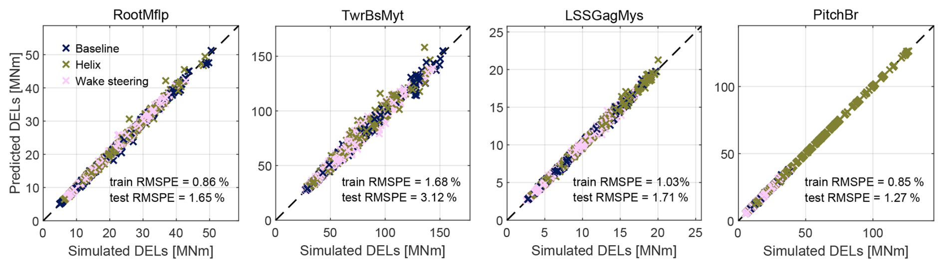
Figure 9 Scatterplots of the test data compared to predictions of the GP model based on the test input data for four of the considered structural components. The fit of the predictions for both training and test data is provided in the figure in terms of RMSPE. The GP predictions and test data samples are grouped based the control strategy that was employed (i.e., baseline control, the helix method, or wake steering).

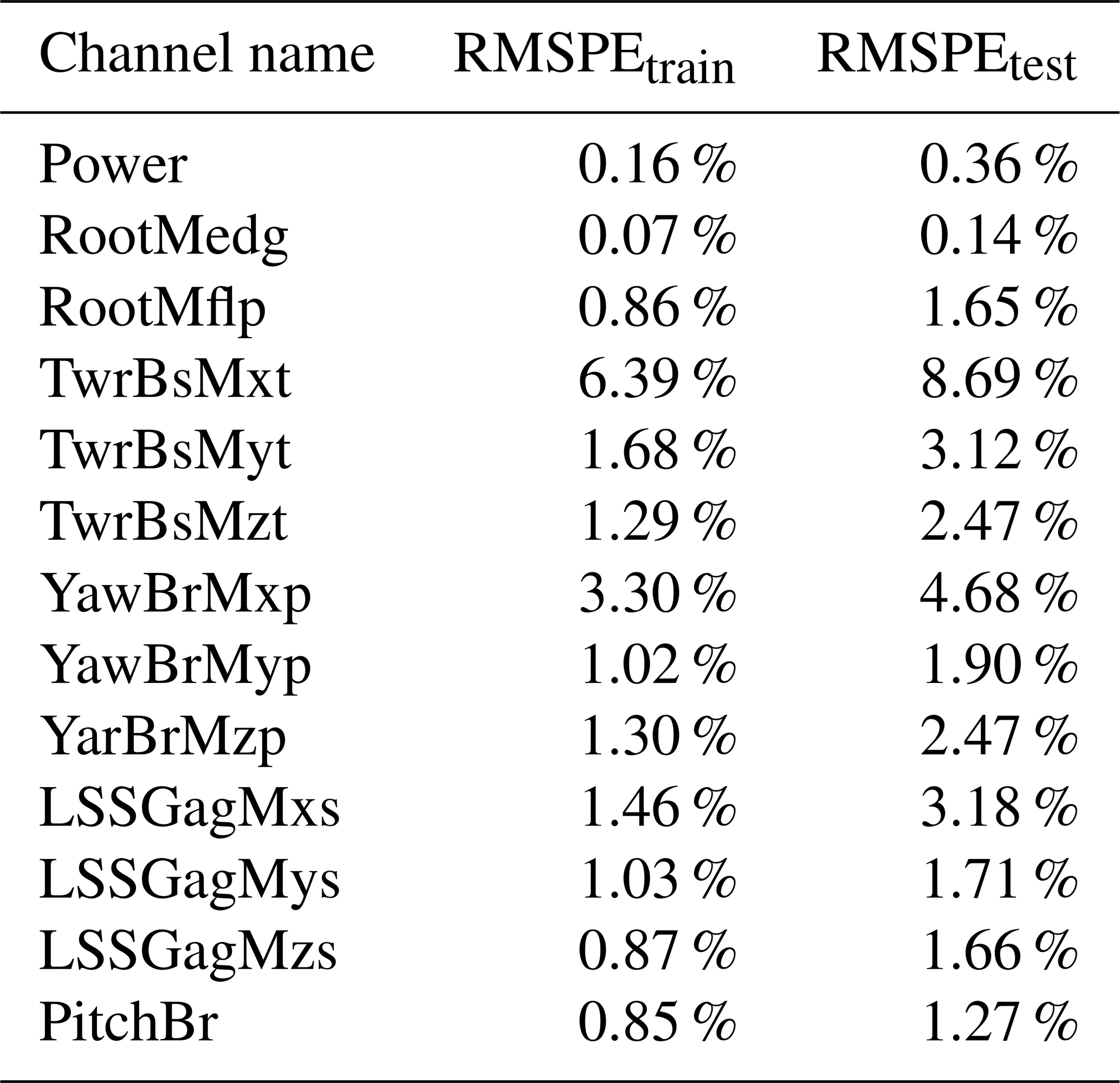
For the blade root, low-speed shaft, and pitch bearing components, we observe similar prediction accuracies. In the case of the tower base, the surrogate model performs slightly worse, with some outliers visible in the higher load range. For each component, the surrogate model shows a slight decline in prediction capabilities for the test set compared to the training set, although the differences are minimal. To assess whether prediction accuracy varies across control strategies, Fig. 9 distinguishes between baseline, helix, and wake steering cases. No systematic bias is observed for any particular strategy, confirming that the surrogate model generalizes well across all operating conditions included in the training data. For the remaining components, the accuracy of the surrogate models is provided in Table 4. For the majority of the components, the fit with the test data is in the same range. The only outliers are the tower components in the side–side direction. The mismatch between the prediction and test data is seen primarily in the higher load range, corresponding to scenarios with full wake overlap. Adding more turbulence seeds to the loads database is expected to improve the prediction performance of the load surrogate model.

Table 4 Prediction performance of the surrogate models expressed as RMSPE for input data from the training and test sets, respectively.

4.2 Case study

In this section, we will perform a case study featuring a two-turbine array. The upstream turbine (T1) is operating in freestream conditions, and the second turbine (T2) is located 5 D downstream. Different control strategies will be tested on the upstream turbine, consisting of baseline (greedy) control and the helix method with different pitch amplitudes.

For the comparison, we used cross-stream flow slices of the streamwise velocity and turbulence intensity from the LES. An example of the flow slices is shown in Fig. 10. For T1, a flow slice of the undisturbed velocity field is selected with a hub-height velocity of U=10 m s⁻¹. This velocity field is subsequently decomposed into the four sector-averaged quantities that are used for the load surrogate model. The same approach is used for the turbulence intensity profiles. For T2, we use the flow slices extracted at 5 D in the case when the upstream turbine is operating with baseline control, as well as the helix method with amplitudes of A_β=2.0° and A_β=4.0°. To replicate the effect of different alignment angles between the two turbines, we vary the lateral displacement d of the extracted rotor plane for T2.

Figure 10 Example of the inflow velocity slices used for generating the load database. From left to right, we see the undisturbed inflow of T1, the inflow of T2 when T1 is using baseline control, and the inflow of T2 when T1 is using the helix method with increasing pitch amplitudes. The rotor plane is illustrated with the four sectors that are used as input for the load surrogate model.

The DELs of several components for the different cases as predicted by the load surrogate model are presented in Fig. 11. In all plots, the predictions are compared to the simulated loads from the test set and are seen to match well. The figure also contains the confidence interval of the GP's prediction. For each component, except the tower base (Fig. 11b), the surrogate model is very confident of the predicted mean. Note that the confidence interval here refers to the uncertainty in the expected mean function, and does not capture the variation in loads from the different turbulence seeds.

The first column of the figure shows the effect of a rising helix pitch amplitude on the fatigue loads. All components in the figure show an increase in loads, but the most significant rise is seen for the pitch bearings in Fig. 11d. This is evident from its definition in Eq. (10), which considers the degree of travel of the bearing δβ. For the blade root (Fig. 11a) and low-speed shaft (Fig. 11c), the increase in load with the helix is on the same order of magnitude as a turbine experiences when operating in a wake. Moving on to the loads of the downstream turbine (T2), we see a double Gaussian shape for the blade root bending moment when T1 uses baseline control. This load profile originates from operation with partial wake overlap, where the blades experience both high and low wind speeds over a single rotation. When the helix method is active on T1, the shape remains the same, but the peaks and the valley in the middle see a small rise for increasing pitch amplitudes. This rise can be seen as the combined result of a higher wind speed and turbulence downstream with the helix. In the case of the tower base (Fig. 11d), the loads initially decrease for a helix amplitude of 2.0°. This results from the turbine's blade passing frequency (3P) coinciding with the first tower mode at lower wind speeds (Zahle et al., 2024). As the wind speed increases with the helix, the 3P frequency moves away from the tower mode. Then, as we apply higher pitch amplitudes, the load increases once more due to the additional turbulence in the wake. Both the low-speed shaft and pitch bearings see a small increase in loading with the helix method, although for the latter, the increase in loading is insignificant when compared to the additional loading seen for T1.

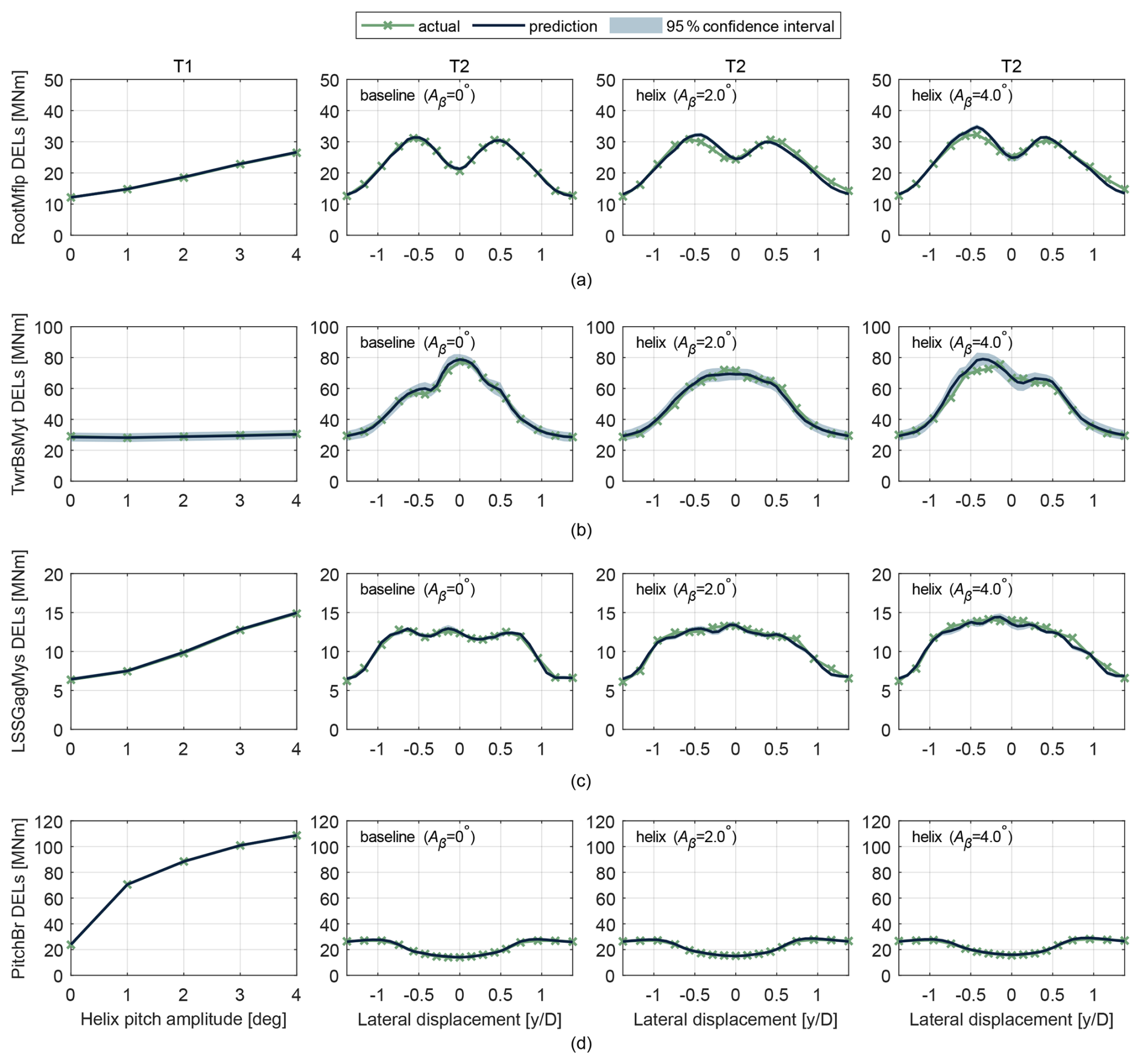
Figure 11 Comparison of loads from the simulated data against predictions from the surrogate model. The first column focuses on the effect of pitch amplitude with the helix method on the loading of the upstream turbine (T1). The remaining columns consider the loads of the downstream turbine (T2) as a function of lateral displacement with respect to T1, and for different control strategies of T1. These strategies consist of baseline control, as well as the helix method with pitch amplitudes of A_β=2.0° and A_β=4.0°, respectively. The components that are considered consist of the blade root (a), tower base (b), low-speed shaft (c), and the pitch bearing (d).

Previously, we only considered the effect of the helix method on the fatigue loading of the two turbines. As with the various load channels, we also trained a surrogate model to predict generator power (extracted from the OpenFAST simulation database) based on inflow sectors. In this way, we quantify the cost in terms of loads associated with a potential energy gain. For this purpose, we consider the same two-turbine array as before and evaluate the performance within a small wind direction range of $\mathit{\varphi }=\mathit{\{}-\mathrm{4}:\mathrm{0.5}:\mathrm{4}\mathit{°}\mathit{\}}$ where the helix will typically be active. The helix pitch amplitude is varied between 0 and 4°. The wind direction misalignment is achieved by feeding the same angle as yaw misalignment to the surrogate models and by displacing the incoming flow field for T2 as indicated in Fig. 10. The resulting load and power estimates are presented in Fig. 12. The average total power of the two turbines is computed for each pitch amplitude by weighting the individual estimates with a Gaussian distribution of the wind direction as proposed by Rott et al. (2018):

$$\begin{array}{}\text{(14)}& {\overline{P}}_{\text{array}}=\sum _{\mathit{\varphi }=-\mathrm{4}\mathit{°}}^{\mathit{\varphi }=\mathrm{4}\mathit{°}}{p}_{\mathit{\varphi }}\left(\mathit{\varphi }\right)\cdot {\widehat{P}}_{\mathrm{array}}\left(\mathit{\varphi },\mathit{\gamma },A_{\mathit{\beta }}\right).\end{array}$$

The Gaussian distribution p_ϕ uses a standard deviation of σ_ϕ=2.5° and is discretized over the selected wind direction range with 0.5° increments. Likewise, the average DELs of each component are determined by weighting the predictions with the Gaussian distribution. Analyzing the turbine array in this way replicates the effect of a realistic time-varying wind direction signal.

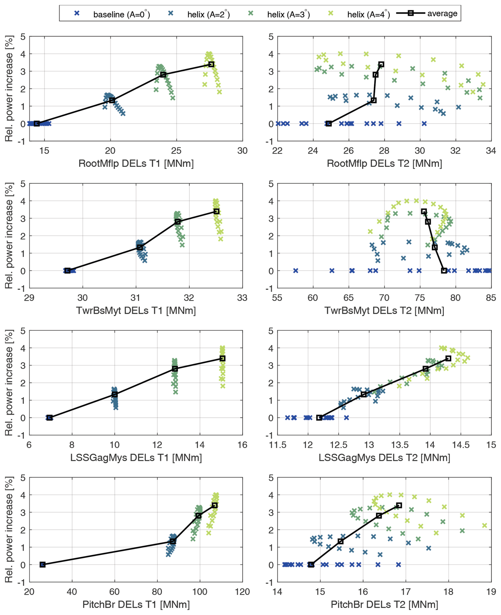
Figure 12 Tradeoff between the relative power increase ($[P_{\mathrm{WFFC}}/P_{\mathrm{BL}}-\mathrm{1}]\times \mathrm{100}\mathit{\%}$) and loads of a two-turbine array as predicted by the surrogate model. The left column shows the loads of T1, and the right column those of T2. The average relation between power gain and loads is determined by weighting the estimates with a Gaussian wind direction distribution.

The first column in Fig. 12 shows the tradeoff in loads and power gain for the upstream turbine (T1). For the helix cases, the relative power increase is compared to the baseline case with the same wind direction misalignment. The load differences in each of the control cases are small, as it is primarily influenced by wind direction and thus small yaw misalignments. However, the power gain varies to a greater extent depending on the wind direction angle. For increasing pitch amplitudes, the average power gain increases but so do the loads of each component due to the periodic pitch actuation. The results from the downstream turbine show greater load variations across changing inflow conditions. Similar to T1, we also observe higher loading for increasing pitch amplitudes, due to the additional turbulence introduced in the wake. Only in the tower base load channel do we see a decrease in loading as pitch amplitude increases, indicating that not all loads are driven by turbulence but can also be affected by the average inflow wind speed. For the blade root, tower base, and low-speed shaft, the increased loads of T1 are in the same range as those experienced by T2. This means that the loading of these components is dominated by wake conditions. The same does not apply to the pitch bearings, which see a large increase in loading on the actuated turbine (T1), whereas the bearings of T2 are barely affected.

The maximum power gain achieved in this scenario is approximately 4 %, which is below the maximum gain achieved in Sect. 3.2. The difference in gain is explained by the different wind speed for this case study (i.e., U_∞=10 m s⁻¹ instead of U_∞=8 m s⁻¹) and the simulation environment. The latter relates to the efficiency loss the upstream turbine experiences when applying the helix. With AMR-Wind, a pitch amplitude of 4° results in a power loss of 2 %, whereas the same pitch amplitude results in a power loss of 5 % when simulated with standalone OpenFAST. This difference is attributed to the different aerodynamic modeling approaches underlying each simulation environment. Where AMR-Wind resolves blade loading directly from the LES flow field via the actuator line method, standalone OpenFAST relies on blade-element momentum theory with a dynamic inflow correction. As the surrogate model for generator power is trained on standalone OpenFAST data, this modeling difference propagates directly into its power loss predictions for T1.

5 Conclusions

This paper investigated the performance of the helix wake-mixing method from both yield and loading perspectives. The motivation for this work is the great computational effort required to assess these aspects, which primarily rely on large eddy simulations. To reduce the number of simulations and make this problem more tractable, we adopted a data-driven modeling approach with GP regression. First, the power output of a two-turbine array was modeled as a function of the actuation frequency and amplitude, using the GP both to characterize where and to what extent the helix method is effective and to guide the selection of simulation settings toward near-optimal control settings. The data for this model were generated with LES of the IEA 22MW reference wind turbine. Second, we presented a load surrogate model for this turbine that predicts fatigue loads for wind farm flow control techniques, such as the helix method, based on the inflow and control settings.

The framework for determining optimal settings for the helix method used the power output of turbines in the large eddy simulations. These simulations were carried out with a conventionally neutral boundary layer with low turbulence levels, similar to conditions encountered on the North Sea. Time series of the turbine power were divided into 10 min segments and averaged over these time periods. These average power measurements were then given to a GP model as training data, along with the control inputs in the form of the helix frequency (expressed as the dimensionless Strouhal number) and pitch amplitude. The training data showed the variability in power gain that wind farm flow control techniques encounter, which was also captured by the GP model in the form of prediction uncertainty. After some initial simulations with random frequencies and amplitudes to explore the control space of the model, additional simulations were performed to enhance the power yield of the two turbines. Finally, the optimal settings for this configuration and the ambient conditions were determined using a limited number of simulations. The optimal power gain of 7.5 % was achieved with Strouhal number St=0.25 and blade pitch amplitude A_β=4° for the counterclockwise helix implementation. The clockwise implementation of the helix (i.e., the orientation of the wake spiral) achieved power gains of only 3 %. The current framework can also be extended to include different ambient conditions, such as wind speed, turbulence intensity, and atmospheric stability conditions.

Large eddy simulations also formed the basis of the load surrogate model presented in this paper. Building on previous work on efficient fatigue load models (e.g., Guilloré et al., 2024), a model was developed to predict the fatigue loads of the IEA 22 MW turbine when wake-mixing control methods, such as the helix method, are applied. Cross-stream velocity slices of turbine wakes were extracted from the LES and converted into input files for aeroelastic simulations to capture the periodic nature of the wake. This approach enabled us to simulate various levels of wake overlap and create a database comprising multiple scenarios. The time series from the aeroelastic simulations of several structural components were then processed into 1 Hz equivalent fatigue loads using a rainflow counting algorithm. The inflow was converted into four sector-averaged values for both velocity and turbulence. The sector-averaged inflow data, along with the wind farm control metrics (i.e., helix pitch amplitude and yaw misalignment angle), are used as inputs to a surrogate model based on GP regression. The load database was divided into a training and a test set, and the prediction accuracy was evaluated using the root mean square percentage error (RMSPE). For the majority of the load channels, the surrogate model achieved RMSPE levels of 3 % or lower when using input data from the test dataset.

Finally, the load surrogate model was tested in a case study with two wind turbines separated by a distance of 5 D. The inputs for the load surrogate model were extracted from the LES: velocity slices of the undisturbed wind field for the upstream turbine and slices of the wake extracted at 5D for the downstream turbine. The helix method was applied to the upstream turbine with different amplitudes ranging from A_β=0° (baseline) to A_β=4°. For the case study, we considered several load channels, for which the predictions agreed well with the test data. Raising the helix amplitude resulted in increased fatigue loads for most load channels in both turbines but most significantly in the upstream turbine. However, apart from the pitch bearings, the absolute loads of the upstream turbine were of the same order of magnitude as those experienced in the wake. The case study was concluded by evaluating the performance gain of the two turbines in terms of power yield and the additional cost in terms of loads experienced by the turbines. For the blade root, tower base, and low-speed shaft components, the power gain and increased loads appear to be well balanced. However, the pitch bearings of the upstream turbine pay a high cost for this increase in power yield.

In summary, this paper employed data-driven modeling, specifically GP regression, to optimize controller settings and predict fatigue loads using the helix wake-mixing method. Future work will focus on coupling the load surrogate model with steady-state engineering wake models to evaluate the helix method on a wind farm level. Previous studies have investigated the potential yield increase associated with the helix method by developing velocity deficit and added turbulence models that depend on the helix pitch amplitude (Dammann et al., 2025a, b). However, these investigations did not consider the effect of wind farm flow control methods on fatigue damage. The current study can be used to bridge this gap and account for the increased loading during the wind farm control optimization phase and hence achieve a balance between power gain and increased fatigue loads. Moreover, since the load surrogate model was also trained to account for yaw misalignment and skewed inflow, it offers flexibility for application in other WFFC strategies beyond the helix, such as wake steering, which was not directly assessed in this study.

Appendix A: Nomenclature and abbreviations

A1 Nomenclature

Latin symbols are listed first in alphabetical order, followed by Greek symbols.

Aβ	Helix pitch amplitude	USA	Sector-averaged wind speed
D	Rotor diameter	$\overline{u}$	Local time-averaged streamwise velocity
d, Δy	Lateral displacement between the wake and the rotor plane	u′, v′, w′	Instantaneous streamwise, transverse, and vertical velocity fluctuations
fβ	Blade pitch actuation frequency	x, x*	Gaussian process training and test input locations
fe	Wake-mixing excitation frequency	y, y*	Gaussian process training output data and inferred test output
fr	Rotor rotational frequency	z	Height
K	Gaussian process covariance (kernel) matrix	z0	Surface roughness length
Leq1Hz	1 Hz damage equivalent load	zH	Turbine hub height
Li	Load amplitude of rainflow bin i	zi	Boundary-layer inversion height
LPB	Pitch bearing damage equivalent load
Medg	Blade root edgewise bending moment	βi	Blade pitch reference signal of blade i
Mflp	Blade root flapwise bending moment	β*	Optimal collective pitch angle
m	Wöhler slope (S–N curve) exponent	Γ	Atmospheric lapse rate
Nbins	Number of rainflow-counting bins	γ	Yaw misalignment angle
Ncycles	Number of 1 Hz cycles per 10 min interval	Δh	Boundary-layer inversion thickness
Nref	Reference degree of pitch travel per 10 min interval	Δt, ΔtLES, ΔtOF	Simulation time step (general, LES, OpenFAST)
Nsteps	Number of simulation time steps	Δθ	Capping inversion strength
NWT	Number of wind turbines	Δx, Δxr	Base and refined LES cell size
ni	Number of load cycles in rainflow bin i	δβ(k)	Pitch travel at time step k
PBL	Turbine power under baseline control	ϵ	Gaussian actuator-line force-projection kernel width
PWFFC	Turbine power under wind farm flow control	θ	Potential temperature
R	Rotor radius	θ0	Ground potential temperature
r	Radial coordinate on the rotor plane	μ*, Σ*	Gaussian process posterior mean and covariance
St	Strouhal number	μ, σ2	Gaussian process estimate mean and variance
Tβ	Period of the pitch actuation signal	σn	Gaussian process noise hyperparameter
Tr	Rotor rotation period	ϕ	Wind direction / wind veer angle
t	Time	ϕlat	Latitude of the simulation domain
U	Wind speed	χ	Radial (azimuthal) position of the pitch bearing (Eq. 10)
U∞	Freestream (inflow) wind speed	ψ	Rotor-plane azimuth angle used in the sector-averaging integral
Urat	Rated wind speed	ψ0,i	Azimuth angle of blade i at t=0

A2 Abbreviations

Note: individual load-channel names (e.g., RootMflp, TwrBsMyt, LSSGagMys, PitchBr) are defined separately in Table 2.

ALM	Actuator line method
AMR-Wind	Adaptive Mesh Refinement for Wind (LES simulator)
ANN	Artificial neural network
CCW	Counterclockwise (helix rotation direction)
CNBL	Conventionally neutral boundary layer
CW	Clockwise (helix rotation direction)
DEL	Damage equivalent load
GP	Gaussian process
HPC	High-performance computing
LES	Large eddy simulation(s)
LUT	Lookup table
PBDEL	Pitch bearing damage equivalent load
PCE	Polynomial chaos expansion
POD	Proper orthogonal decomposition
RMSPE	Root mean square percentage error
ROSCO	Reference open-source controller
SATI	Sector-averaged turbulence intensity
SAWS	Sector-averaged wind speed
SIC	Static induction control
TI	Turbulence intensity
WFFC	Wind farm flow control