Dynamic response and loads analysis of a large offshore wind turbine under low-frequency wind fluctuations

We investigate the impact of low-frequency wind fluctuations on the loads and response of a large reference offshore wind turbine. Synthetic wind fields containing low-frequency fluctuations down to 1 h⁻¹ are used in aeroelastic simulations with the HAWC2 code. The dynamic response and damage equivalent loads (DEL) for tower and blade moments are evaluated. Both monopile and floating configurations are tested against three wind fields: (i) high-frequency turbulence (3D), (ii) combined low- and high-frequency turbulence (2D+3D), and (iii) high-frequency turbulence scaled to match the measured standard deviation. Low-frequency fluctuations increase DEL for the fore–aft and flapwise moments at the tower base and the blade root, especially at low wind speeds. These are out-of-plane bending moments caused by longitudinal forces. Torsional moments, such as tower top yaw, exhibit reduced DEL across most wind speeds due to increased coherence. The strongest dynamic response to low-frequency turbulence occurs in the tower fore–aft and blade root flapwise moments at frequencies below $\mathrm{2}\times {\mathrm{10}}^{-\mathrm{3}}$ Hz. For the floating turbine, the platform's surge and pitch motions, and the windward mooring line tension, show pronounced responses. This study underscores the importance of accounting for low-frequency wind fluctuations when simulating the loads and response of large offshore wind turbines.

1 Introduction

A rapid expansion in global offshore wind power capacity is underway, driven by the need to achieve sustainability and clean-energy targets. Offshore wind energy projects offer higher capacity factors due to the more reliable and robust wind resources found in the marine atmosphere. Technological advancements in the manufacturing of offshore wind turbines have led to a pronounced reduction in the cost of offshore energy. Modern offshore wind turbines are considerably larger than their onshore counterparts. Onshore turbines experience inflow turbulence that is mainly three-dimensional, as described by the standards. Conversely, offshore turbines experience weaker three-dimensional turbulence, while low-frequency structures are relatively more dominant. These structures influence the fatigue loading response of wind turbine towers and blades. Furthermore, the response of floating offshore wind turbines is even more susceptible to low-frequency wind fluctuations due to more degrees of freedom and low natural frequencies of rigid-body motions (Doubrawa et al., 2019).

In the wind turbine design process, synthetic turbulent wind fields are used in aero-hydro-servo-elastic codes to analyze the effects of atmospheric turbulence on the loads and dynamic response of different system components. International Electrotechnical Commission (IEC) standards (IEC, 2019) recommend two turbulence models to generate wind fields for the turbine design process: (i) the Mann uniform shear model (Mann, 1994, 1998) and (ii) the Kaimal spectral model with exponential coherence (Kaimal et al., 1972; Davenport, 1977). The main advantage of these two models over other high-fidelity methods for generating turbulent wind fields, such as large eddy simulations (LES), is their significantly lower computational cost. Their main drawback is that these models assume neutral stratification and represent stationary onshore atmospheric conditions. The marine atmosphere is characterized by large-scale quasi-two-dimensional turbulent eddies with timescales exceeding 500 s (Syed and Mann, 2024a; Cheynet et al., 2018), which the recommended IEC turbulence models cannot accurately capture. Here, the 2D turbulence is characterized by eddies with a large aspect ratio, i.e., the ratio of the horizontal to the vertical length scales.

Numerous studies have highlighted the impact of large-scale coherent structures or low-frequency wind fluctuations on the response of large offshore wind turbines. For instance, Bachynski and Eliassen (2019) investigated the global motion responses of an NREL 5 MW reference floating wind turbine and found that it is highly sensitive to low-frequency wind fluctuations, resulting in increased floating platform surge, pitch, and mooring line responses. They utilized the proper orthogonal decomposition (POD) method to decompose the input wind fields from the Mann and Kaimal models into coherent structures. It has been demonstrated that only a few of the lowest POD modes can characterize the low-frequency wind fluctuation response in wind turbines (see Eliassen and Andersen, 2016; Saranyasoontorn and Manuel, 2005). Nybø et al. (2021b) and Nybø et al. (2022) concluded that the large-scale coherent structures are responsible for increased tower base fore–aft moments and blade root out-of-plane bending moments in the fixed-bottom wind turbines and additionally increased surge, pitch, and mooring line responses in floating wind turbines. These studies used standard turbulence models, suggesting that low-frequency wind turbulence may be underestimated or inaccurately modeled. Nybø et al. (2021a) and Nybø et al. (2022) also compared the standard Mann and Kaimal turbulence models with the LES and TIMESR turbulence models. The TIMESR turbulence model is a feature of the TurbSim tool (Jonkman, 2014), developed by NREL, USA. It requires a time series of wind measurements as an input and outputs a constrained turbulence field. Only the TIMESR turbulence model could match the low-frequency energy observed in the measured wind spectra. However, the lowest frequency in these comparisons was 0.0017 Hz, corresponding to a timescale of less than 10 min. As documented in previous studies (Syed and Mann, 2024a), the mesoscale turbulence or low-frequency wind fluctuations exhibit significant energy at frequencies below $\mathrm{2}\times {\mathrm{10}}^{-\mathrm{3}}$ Hz. The implications of wind turbulence at frequencies below $\mathrm{2}\times {\mathrm{10}}^{-\mathrm{3}}$ Hz on the loads and dynamic responses of wind turbines remain largely unexplored.

In our study, we use the low-frequency wind turbulence model (hereafter, the “2D turbulence model”) presented by Syed and Mann (2024a). This model accurately predicts low-frequency longitudinal (u) and lateral (v) wind fluctuations within the mesoscale range, i.e., well below 10⁻³ Hz. We combine the 2D turbulence model with the Mann uniform shear model (hereafter, the “3D turbulence model”) to simulate turbulence in the frequency range down to 1 h⁻¹. The model parameters are obtained from the undisturbed wind data collected at the FINO1 research platform in the North Sea. We investigate the impact of low-frequency wind fluctuations by evaluating the fatigue loads and aerodynamic response of the International Energy Agency (IEA) 15 MW reference wind turbine (Gaertner et al., 2020). The reference turbine design is available in two configurations: a fixed-bottom design with a monopile embedded in the soil and a floating design with a semi-submersible floating platform supported by mooring lines. The IEA 15 MW wind turbine is an open-source design that has undergone various response analyses and design studies (Mendoza et al., 2022; Mahfouz et al., 2021; Niranjan and Ramisetti, 2022; Nybø et al., 2022; Rinker et al., 2020; Ramos-García et al., 2022).

In this study, we focus on evaluating the damage-equivalent loads (DEL) associated with blade and tower moments and how they respond to low-frequency wind turbulence. We also investigate the rigid-body dynamics of floater motions in the floating configuration of the IEA 15 MW wind turbine. Furthermore, we compare the aerodynamic loading and response under 2D+3D turbulent wind fields with a standard turbulence model and with a 3D-only turbulence model based on the Mann uniform shear model. Section 2 of this article describes the data and methodology employed. A brief description of the IEA 15 MW wind turbine in both monopile and floating configurations is presented. The procedure to generate synthetic wind fields containing 2D and 3D turbulence using the parameters obtained from FINO1 is also described. Additionally, the simulation setup is presented, including details of the aeroelastic code. Sections 3 and 4 contain loads and dynamic responses of the wind turbine in monopile and floating configurations, respectively. This is followed by the Discussion and Conclusion sections, which highlight and discuss the important outcomes of this analysis.

2 Data and methodology

2.1 Wind turbine data

The definition of the IEA 15 MW offshore reference wind turbine is given by Gaertner et al. (2020). It is an IEC class 1B, a direct-drive wind turbine with a rotor diameter of 240 m and a hub height of 150 m. The reference wind turbine has a rated wind speed of 10.59 m s⁻¹. Its configuration has a monopile embedment depth of 45 m. The tower and monopile are made up of isotropic steel tubes. The outer diameter of the tower goes from 10 m at the mud line to 6.5 m at the top of the tower (see Fig. 1a). The tower is designed so that the first tower mode is 0.17 Hz, located between the 1P and 3P blade frequencies to avoid excessive excitation.

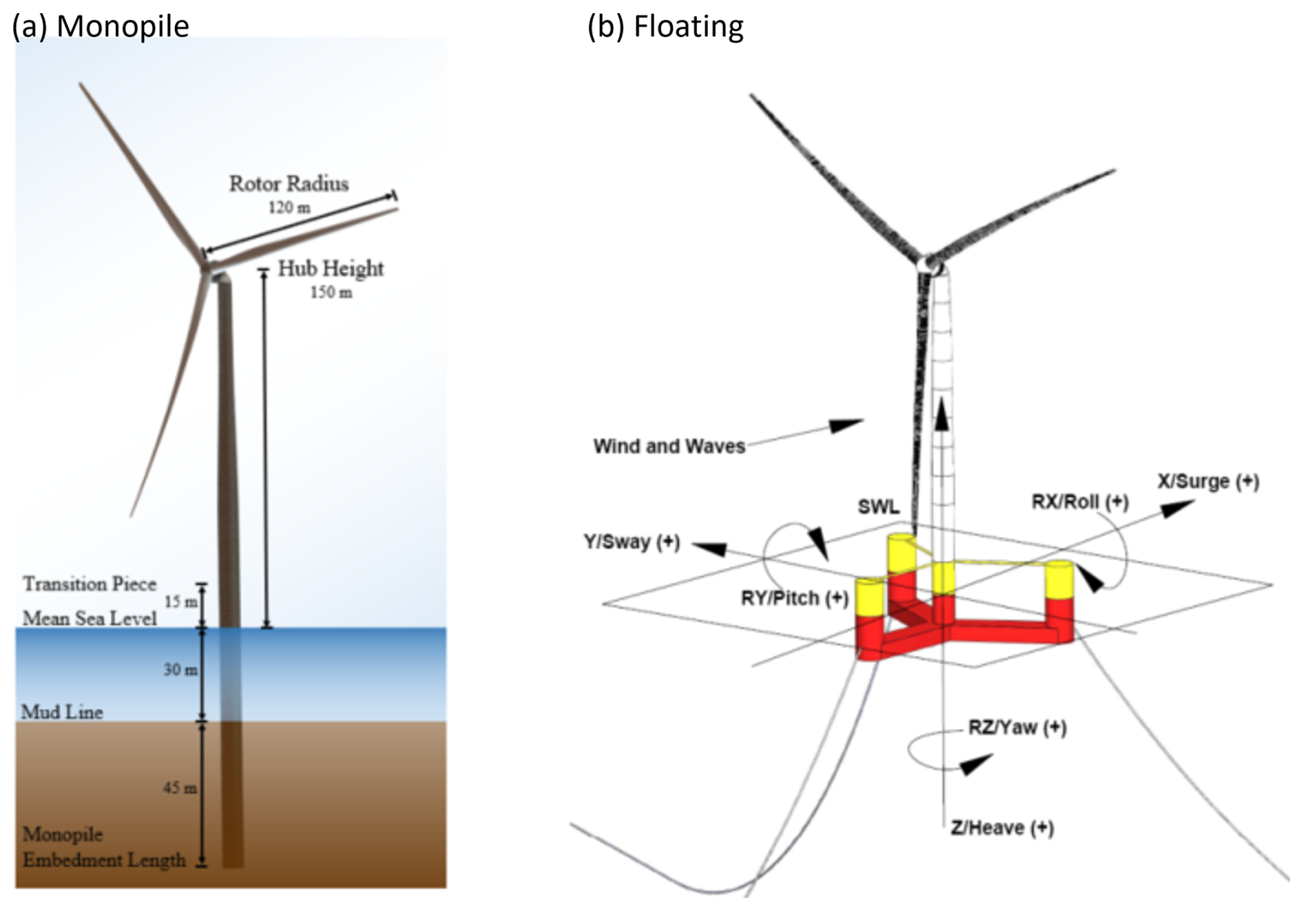
Figure 1 IEA 15 MW reference wind turbine. (a) Monopile configuration and (b) floating configuration with UMaine semi-submersible platform and three mooring lines. Panels (a) and (b) originally published in Gaertner et al. (2020) and Allen et al. (2020), respectively.

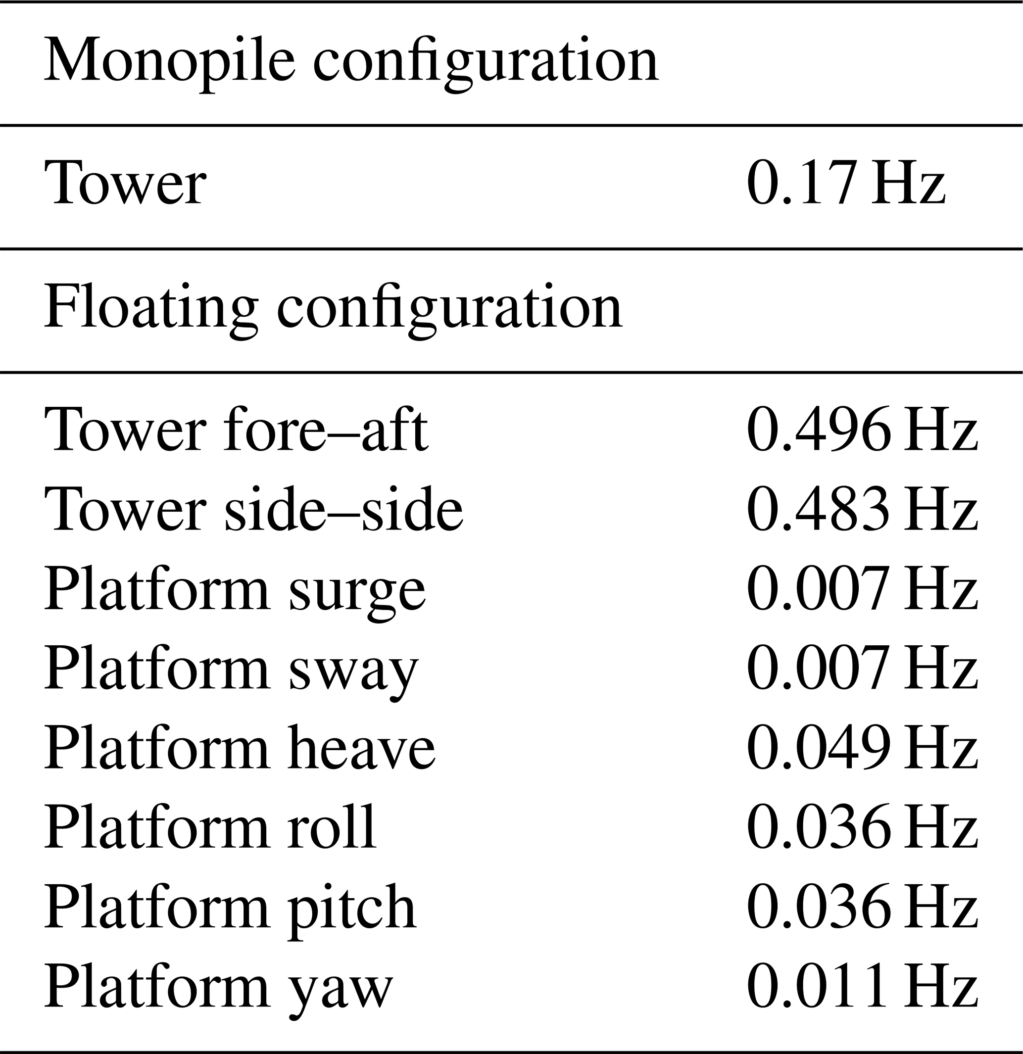
The IEA 15-MW floating configuration comprises a four-column semi-submersible steel platform constrained by a three-line catenary mooring system (Allen et al., 2020). The semi-submersible platform is designed for deployment in water depths of 200 m. The platform has three radial columns with a 120° angle between them and a central column that supports the tower (see Fig. 1b). The three mooring lines are connected to each radial column of the platform via a fairlead about 14 m below sea level. Each mooring line has an unstretched length of 850 m and a linear density of 685 kg m⁻¹. In the floating configuration, higher-stiffness tower design is employed to accommodate the increased inertial and gravity loads from platform motion. The floating tower mass is 47 % higher than the monopile tower. The tower fore–aft and side–side natural frequencies are 0.496 and 0.483 Hz, respectively. These frequencies exceed the 3P frequency of the blades to avoid resonance. A summary of the natural frequencies of the tower and the floating platform, obtained from rigid-body free decay tests, is described in Table 1.

Table 1 Natural frequencies of tower and platform motions in the monopile and floating configuration of the IEA 15-MW offshore reference wind turbine.

2.2 Synthetic turbulent wind field generation

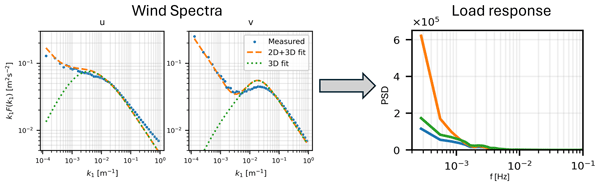
The low-frequency wind turbulence model used in this study is based on a 2D velocity spectral tensor described in Syed and Mann (2024a). The model can accurately predict the mesoscale turbulence where $S\left(f\right)\propto f^{-\mathrm{5}/\mathrm{3}}$. The 2D turbulence model has four input parameters: (i) the azimuthally averaged variance exhibited by low-frequency wind fluctuations, ${\mathit{\sigma }}_{\text{2D}}^{\mathrm{2}}$, (ii) the length scale corresponding to the most dominant large-scale structures, L_2D, (iii) the anisotropy parameter, ψ, and (iv) the attenuation length, usually the boundary layer height z_i. In addition, the scaling parameter (c) for the 2D turbulence model is derived from the magnitudes of both ${\mathit{\sigma }}_{\text{2D}}^{\mathrm{2}}$ and L_2D using Eq. (A1) in Syed and Mann (2024a). A large value of the scaling parameter (c) implies a large variance in the flow field. The 3D turbulence model used here is the Mann uniform shear model Mann (1994), which is one of the models recommended by IEC for wind turbine design load calculations. The 3D turbulence model has three input parameters: (i) the scaling parameter, $\mathit{\alpha }{\mathit{ϵ}}^{\mathrm{2}/\mathrm{3}}$, (ii) the dominant length scale of 3D turbulence, L_3D, and (iii) the anisotropy parameter, Γ. An illustration of the offshore wind spectra recorded at FINO1 under neutral atmospheric conditions is provided in Fig. 2. Here, the measurements show three wind-component spectra for $\stackrel{\mathrm{‾}}{U}=\mathrm{13.5}$ m s⁻¹ at z=81 m. It can be observed that the 3D turbulence model alone cannot describe the low-frequency fluctuations in u and v. Furthermore, the vertical velocity component w has a negligible presence in the mesoscale turbulence, hence the term 2D turbulence.

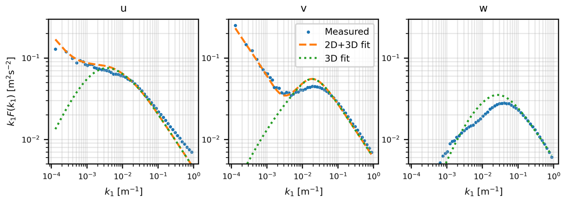
Figure 2 Wind velocity spectra measurements (blue dots) for $\stackrel{\mathrm{‾}}{U}=\mathrm{13.5}$ m s⁻¹ at z=81 m from FINO1 under neutral atmospheric conditions. The 3D turbulence model (Mann spectral model) is fitted (dotted green lines) as well as the 2D+3D turbulence model (dashed orange lines) for u and v components.

Given the parameters, 2D and 3D turbulent wind fields can be generated based on the methods outlined in Syed and Mann (2024b) and Mann (1998), respectively. To generate the synthetic turbulent wind fields, we obtained the turbulence model parameters from the FINO1 test site in the German North Sea. Stability data analysis from FINO1 for the years 2007–2008 revealed that neutral conditions were prevalent more than 40 % of the time (Syed and Mann, 2024a). Hence, in this study, only neutral conditions will be analyzed. To evaluate measured spectra, first, the high-frequency 10 Hz data from the ultrasonic anemometer were divided into 1 m s⁻¹ bins from cut-in to cut-out wind speeds (3–25 m s⁻¹) of the IEA-15 MW reference wind turbine. The number of 1 h time series in each bin is shown in Fig. 4a. Thus, the total number of hours processed is 6226. The spectra of all three wind components were recorded for all 1 h time series, and for each wind speed bin, the power spectra of all three components were averaged. This averaging ensures that the spectra do not contain any random artifacts or non-stationarities and are a true representation of neutral atmospheric conditions at FINO1. The resulting spectra are displayed in Fig. 3. Averaging makes the spectra smoother and more reliable for calculating turbulence model parameters. 2D and 3D turbulence models were fitted to the mean spectra for each wind speed bin using the least-squares method. A summary of the 2D and 3D turbulence model parameters is shown in Fig. 4b–f. Note that the 2D turbulence anisotropy parameter ψ is close to its isotropic value of 45° at all wind speeds. In contrast, the 3D turbulence anisotropy parameter Γ linearly increases with the wind speed. The 2D turbulence scaling parameter c did not change significantly with the wind speed, but the 3D turbulence scaling parameter $\mathit{\alpha }{\mathit{ϵ}}^{\mathrm{2}/\mathrm{3}}$ showed an increase proportional to ${\stackrel{\mathrm{‾}}{U}}^{\mathrm{2}}$. Because these parameters are derived from ensemble-averaged spectra over many hours per bin (the lowest number of hours is 16 for $\stackrel{\mathrm{‾}}{U}=\mathrm{24.5}$ m s⁻¹), the standard error of the mean (SEM) (SEM measures the dispersion of sample means around the true population mean) is negligible for most of the parameters. Consequently, error bars are only plotted for ψ and L_3D, where the SEM was not so insignificant. To generate synthetic wind fields for 2D turbulence, we need additional information about two parameters: the boundary layer height z_i and the length scale of dominant mesoscales L_2D. We assume a boundary-layer height z_i of 500 m and a dominant mesoscale length scale L_2D of 150 km, since these values cannot be obtained from the measurements.

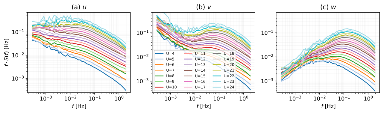
Figure 3 Mean spectra of hourly wind data as a function of frequency f for 1 m s⁻¹ wind speed bins (FINO1, z=81 m) for the three wind components.

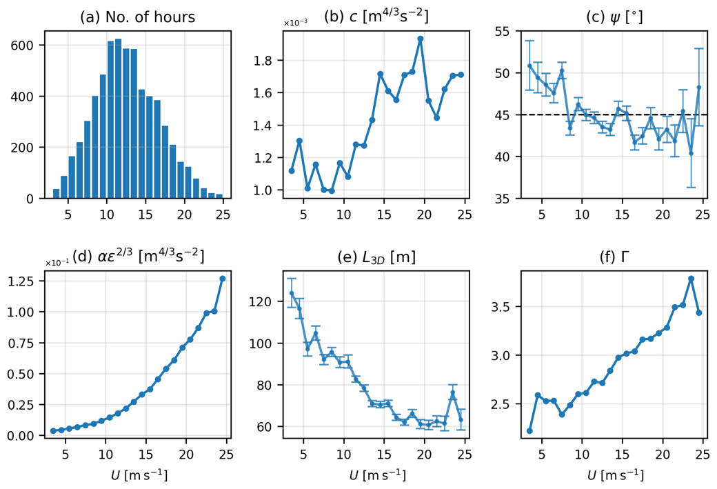
Figure 4 (a) The number of hours representing neutral atmospheric conditions at FINO1 at 81.5 $\mathrm{m}\mathrm{a}.\mathrm{s}.\mathrm{l}.$ in 2007–2008 (total no. of hours = 6226). The data are divided into 1 m s⁻¹ bins from cut-in to cut-out wind speeds (3–25 m s⁻¹). (b) The scaling parameter c of the low-frequency turbulence model is obtained from fitting the spectra. (c) The mean anisotropy parameter ψ was obtained for the low-frequency wind fluctuations. Panels (d), (e), and (f) represent the three Mann turbulence model parameters: αϵ²³, L_3D, and Γ, respectively, obtained from spectral fitting. Error bars in panels (c) and (e) represent the standard error of the mean.

2.3 Aero-elastic simulations

Load simulations were carried out using the HAWC2 aeroelastic code developed at the Technical University of Denmark (DTU). The model is based on a multibody formulation in which each component is represented as a Timoshenko beam, allowing bending and torsional deformation. Pitch control and turbine operation were governed by the DTU Wind Energy Controller (Meng et al., 2020) across three wind speed regions: (i) 3–6.98 m s⁻¹ with constant rotor speed at 5 rpm and torque controlled by a PI controller, (ii) 6.98–10.59 m s⁻¹ with optimal tip-speed ratio and zero blade pitch, and (iii) 10.59–25 m s⁻¹ where rotor speed is limited to 7.55 rpm using a PI pitch controller. For the floating configuration, a tower top velocity feedback loop was included to mitigate pitch instability at rated conditions and above.

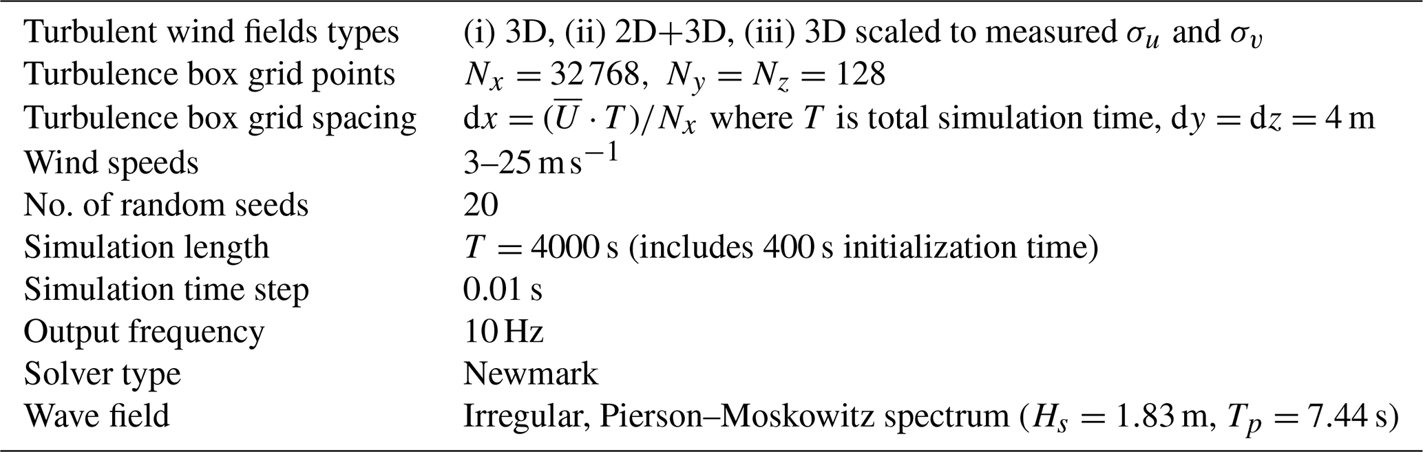
To limit stochastic variability, 20 turbulence realizations based on random seeds were generated for each of the 22 wind speed bins between 3–25 m s⁻¹. We used the same random seeds for the 2D turbulence fields as well as the underlying 3D turbulence boxes. Turbulence boxes consisted of N_x=32 768 and $N_y=N_z=\mathrm{128}$ grid points, with longitudinal spacing dependent on mean wind speed and constant lateral and vertical spacing of $d_y=d_z=\mathrm{4}$ m. This ensured lateral and vertical extents exceeding twice the rotor diameter, avoiding periodicity effects (Mann, 1998; Syed and Mann, 2024b). Three turbulence representations were considered: (i) 3D boxes containing only high-frequency fluctuations, (ii) combined 2D+3D boxes including low-frequency u and v components, and (iii) scaled 3D boxes adjusted to match measured σ_u and σ_v. The unscaled 3D case underestimates velocity variance (Fig. 5), while the scaled case compensates for missing low-frequency energy by amplifying high-frequency content (Syed et al., 2024).

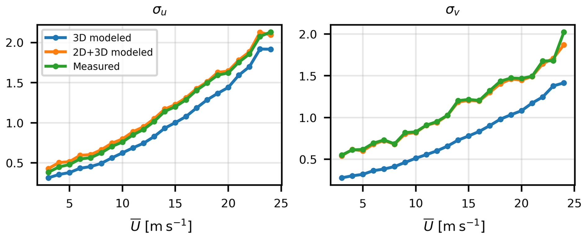
Figure 5 Modeled standard deviations σ_u and σ_v compared to the measured values for 2D+3D model and 3D model.

Wave effects were not investigated; therefore, identical wave conditions were applied in all simulations using a Pierson–Moskowitz spectrum with H_s=1.83 m and T_p=7.44 s, corresponding to a wind speed near 12 m s⁻¹. The complete simulation setup is summarized in Table 2.

Table 2 Simulation setup.

3 Monopile configuration

3.1 Damage equivalent loads

Damage equivalent loads (DELs) are evaluated for five moments: tower base fore–aft, tower base side–side, tower top yaw, blade root flapwise, and blade root edgewise. The 1 Hz DELs are computed by applying rainflow counting to the cyclic load time series to obtain stress ranges S_i, which are converted to DEL using (Syed et al., 2024):

$$\begin{array}{}\text{(1)}& {\displaystyle }{\displaystyle }\text{DEL}={\left({\displaystyle \frac{\mathrm{\Sigma }\left(N_i{S}_i^m\right)}{n_{\text{eq}}}}\right)}^{\mathrm{1}/m},\end{array}$$

where N_i denotes the number of cycles to failure for S_i, n_eq is the signal duration (3600 s), and m is the Wöhler exponent (m=4 for the steel tower and m=10 for the composite blades). Figure 6 presents the mean 1 Hz DELs obtained from 20 realizations at each wind speed. The influence of the turbulence representation is evident for all five moments, with the scaled 3D wind field producing the highest DELs over most wind speeds. This indicates a greater contribution of high-frequency fluctuations to fatigue damage than that of low-frequency turbulence. Relative to unscaled 3D turbulence, inclusion of 2D turbulence increases DELs for moments dominated by longitudinal loading, such as tower base fore–aft (Fig. 6a) and blade root flapwise (Fig. 6d), with a larger effect below rated wind speeds. In contrast, the effect of 2D turbulence on tower base side–side (Fig. 6b) and tower top yaw moments (Fig. 6c) is small, while for blade root edgewise moments (Fig. 6e) the 2D+3D case reduces DELs above rated conditions. The main difference between the rescaled 3D and the 2D+3D wind fields is how the variance is distributed across the frequency and rotor plane (their total variance is the same). The rescaled 3D field amplifies high-frequency fluctuations uniformly, which are spatially incoherent across the rotor, while the 2D+3D field adds energy at low frequencies (below $\mathrm{2}\times {\mathrm{10}}^{-\mathrm{3}}$ Hz), where the longitudinal wind component is coherent across the rotor plane. At low wind speeds, when the pitch controller is not active, spatially coherent fluctuations increase thrust, driving fore–aft and flapwise moments. At wind speeds above the rated wind speed, the pitch controller actively regulates rotor loads and effectively attenuates the response to slow wind variations.

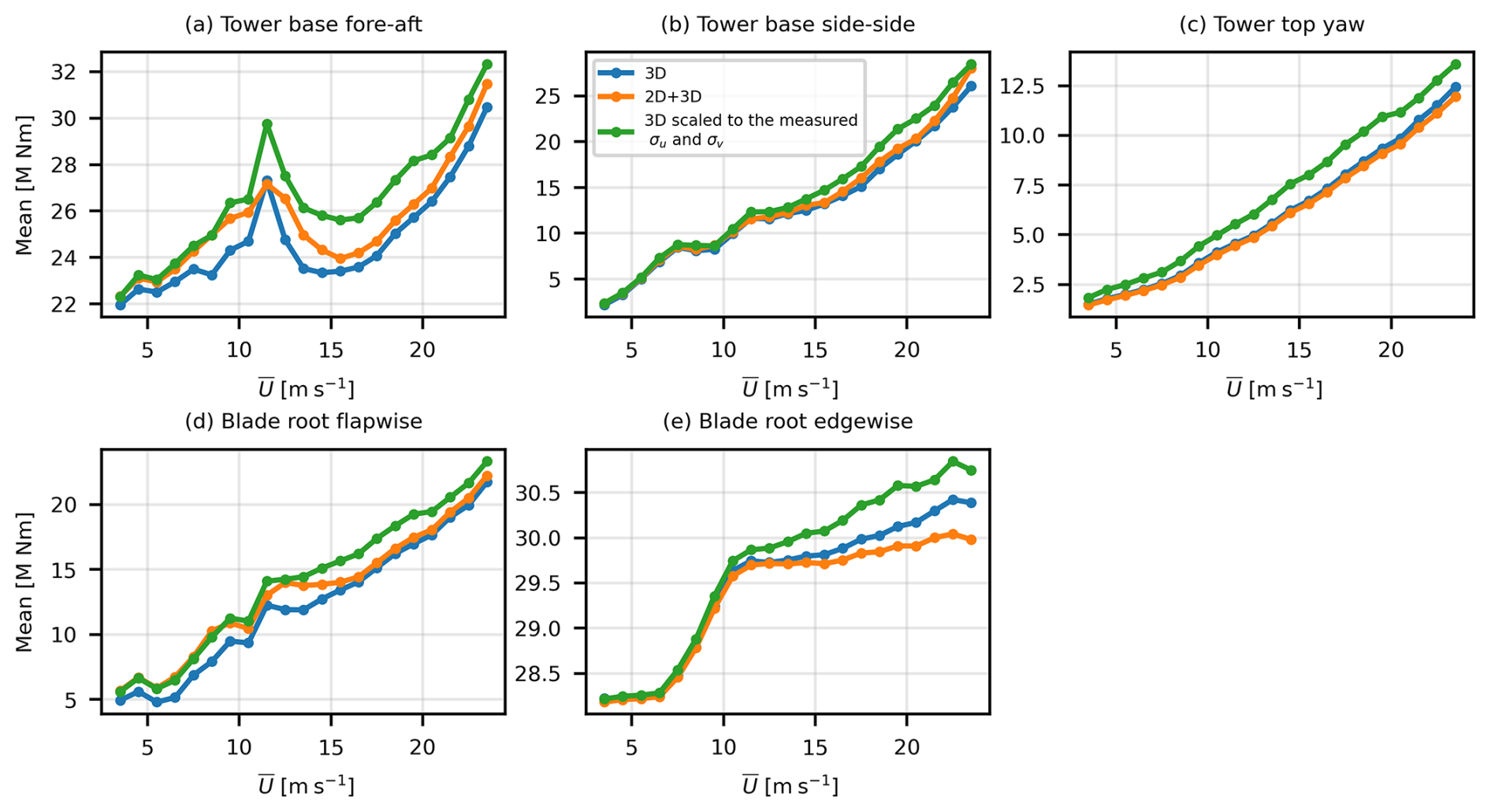
Figure 6 (Monopile IEA 15 MW) 1 Hz DELs of (a) tower base fore–aft, (b) tower base side–side, (c) tower top yaw, (d) blade root flapwise, and (e) blade root edgewise moments. The values represent the mean of 20 simulations at each wind speed.

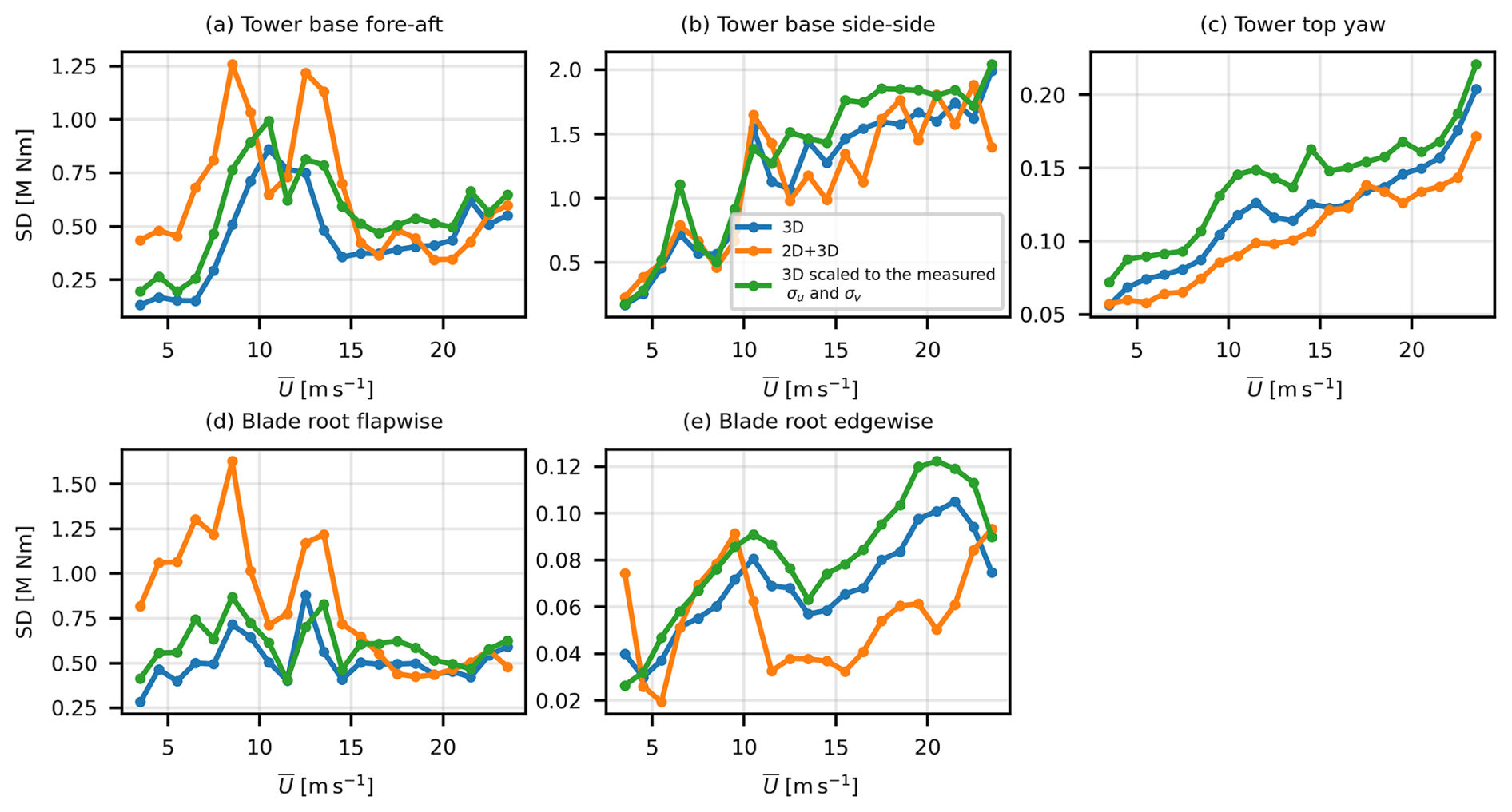
The variability in DELs arising from turbulent wind stochasticity is shown in Fig. 7 through the standard deviation across the 20 seeds. For tower base fore–aft and blade root flapwise moments, large variations are observed for the 2D+3D case at below-rated wind speeds. The tower base side–side moment shows little sensitivity to the turbulence input in either the mean or the standard deviation. For tower top yaw and blade root edgewise moments, the 2D+3D turbulence yields the lowest mean DELs and standard deviations at most wind speeds. These results confirm that 2D turbulence mainly affects fatigue loads associated with longitudinal and out-of-plane moments, particularly below rated wind speed, while reducing DELs for in-plane and torsional moments. The higher seed-to-seed variability in DELs observed for the 2D+3D case in Fig. 7, particularly at low wind speeds, is a consequence of the low-frequency nature of the added turbulence. A simulation length of 1 h contains only a few cycles of fluctuations at periods approaching 500 s. Whether a high-amplitude, low-frequency event occurs within a given realization is therefore highly stochastic, resulting in a large spread across seeds. This highlights that more or longer simulations may be needed to obtain statistically converged DEL estimates when low-frequency wind fluctuations are included.

Figure 7 Same as Fig. 6 but the values represent the standard deviation.

3.2 Dynamic response

The dynamic response of the tower base fore–aft moment at three different wind speeds is shown in Fig. 8. These wind speeds represent three different operating regions of the wind turbine: below-rated speed, 4.5 m s⁻¹, rated wind speed, 10.5 m s⁻¹, and above-rated wind speed, 16.5 m s⁻¹. In the top row of Fig. 8, the full frequency response is shown in terms of the power spectral density (PSD) of the tower fore–aft moment. A peak corresponding to the monopile tower's first mode, i.e., 0.17 Hz, is visible at all three wind speeds. At high frequencies, the scaled 3D turbulence resulted in the highest response values. The impact of 2D turbulence becomes significant at $f<\mathrm{2}\times {\mathrm{10}}^{-\mathrm{3}}$ Hz, corresponding to a time period of 500 s. The bottom row of Fig. 8 displays the PSDs in response to three wind fields at very low frequencies on semi-log plots. The tower's response to 2D turbulence is significant at all wind speeds but becomes strongest at the lowest wind speed, i.e., 4.5 m s⁻¹.

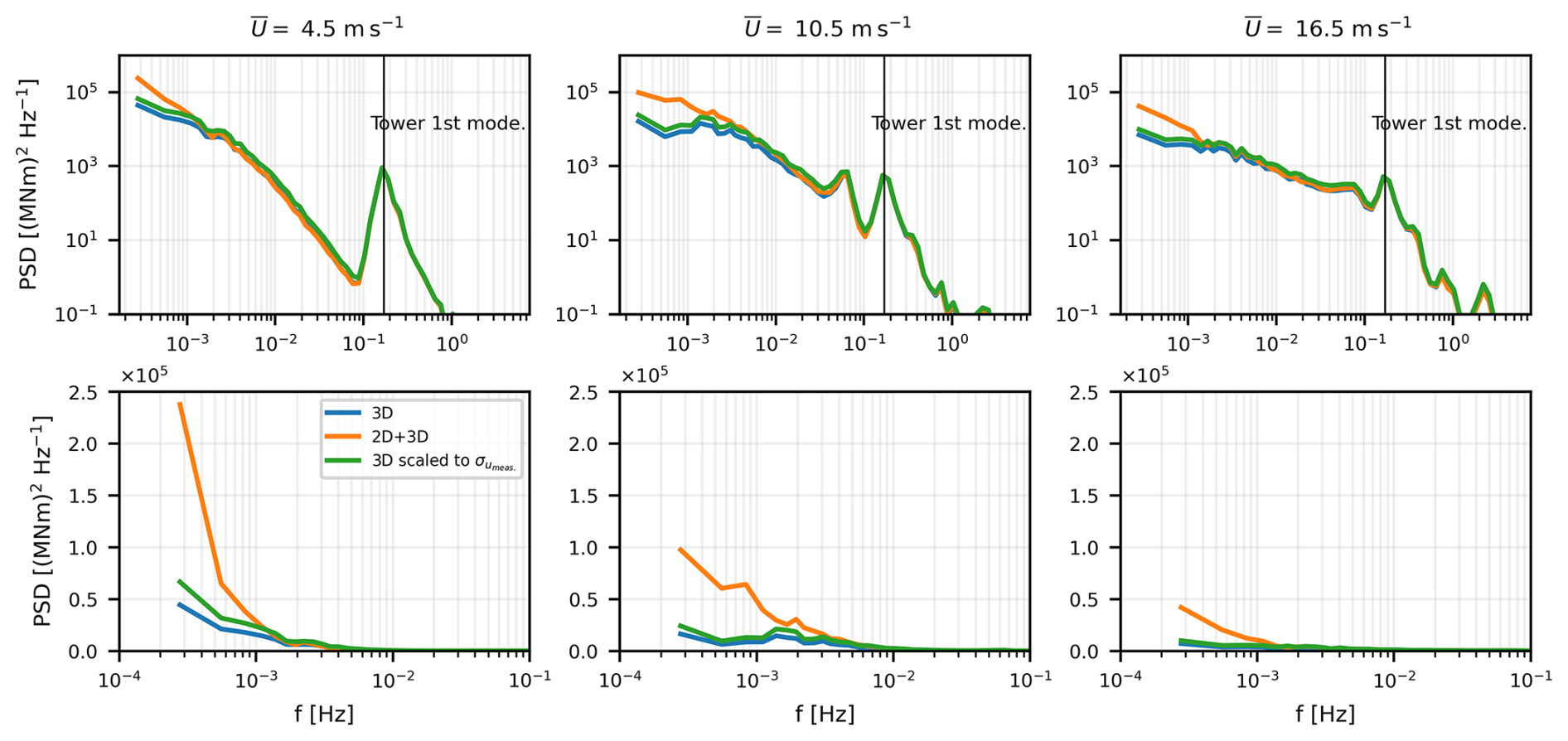
Figure 8 PSD of tower base fore–aft moment in response to 3D, 2D+3D, and scaled 3D turbulent wind fields (monopile configuration). The top row shows the full frequency range, including the high-frequency response on a log–log plot. The straight vertical line at f=0.17 Hz intersects with the tower's first mode peak. The bottom row zooms into the low-frequency response on a semi-log plot.

Figure 9 exhibits similar PSD plots but for the blade flapwise moment in response to different wind fields at three distinct wind speeds. Here, the plots reveal three discernible peaks that align with the 1P, 2P, and 3P rotor frequencies of the turbine. As seen from the bottom row plots in Fig. 9, the PSD of blade root moment in response to 2D turbulence becomes highest for $f<\mathrm{2}\times {\mathrm{10}}^{-\mathrm{3}}$ Hz. Like the tower fore–aft bending moment, the blade root flapwise moment response to 2D turbulence is most pronounced at the lowest wind speed.

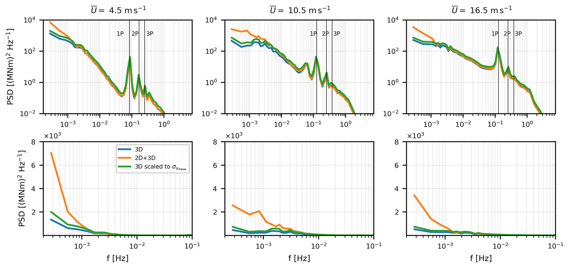
Figure 9 PSD of blade root flapwise moment in response to 3D, 2D+3D, and scaled 3D turbulent wind fields (monopile configuration). The top row shows the full frequency range, including the high-frequency response on a log–log plot. The straight vertical lines intersect with the 1P, 2P, and 3P frequencies of the turbine rotor. The bottom row zooms into the low-frequency response on a semi-log plot.

4 Floating configuration

4.1 Damage equivalent loads

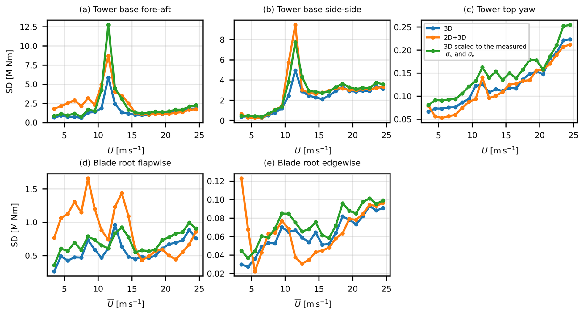
As in the monopile configuration, the highest DELs are obtained with scaled 3D turbulence. Figure 10 displays the mean DEL values for the tower base, top, and blade root moments. The blade root flapwise and edgewise moments are similar in magnitude to those in the monopile configuration. However, the tower bending moments have increased significantly in the floating configuration because of increased inertial and gravity loads and a different tower design. Compared to the unscaled 3D turbulence, the effect of 2D turbulence is higher in the tower base fore–aft and blade root flapwise moments, especially at low wind speed values. The standard deviation in DEL values among different turbulence seeds is shown in Fig. 11. The highest standard deviation is in the tower base moment DELs, while the lowest is observed in the blade root edgewise moment. For the bending moments resulting from longitudinal forces (fore–aft and flapwise), the 2D turbulence exhibits the highest standard deviation values at low wind speeds.

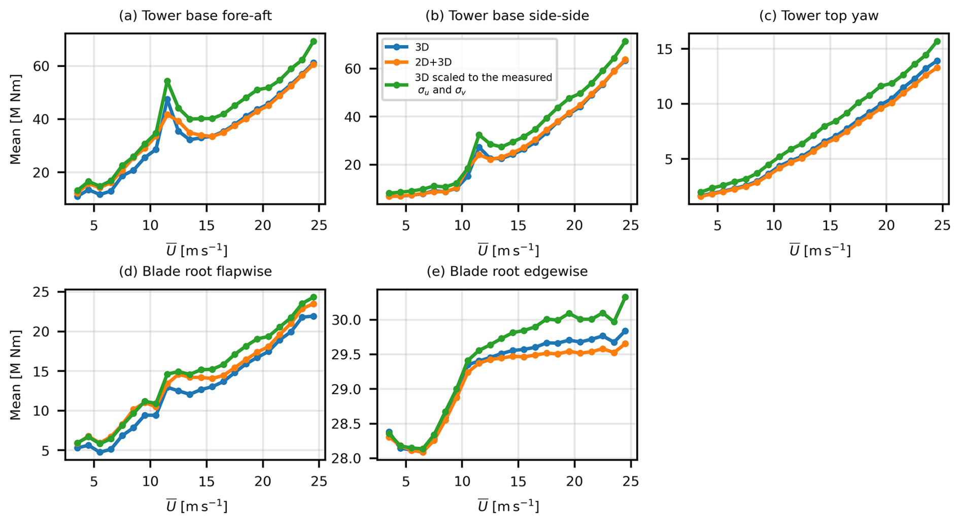
Figure 10 (Floating IEA 15 MW) 1 Hz DELs of (a) tower base fore–aft, (b) tower base side–side, (c) tower top yaw, (d) blade root flapwise, and (e) blade root edgewise moments. The values represent the mean of 20 simulations at each wind speed.

Figure 11 Same as Fig. 10 but the values represent the standard deviation.

4.2 Dynamic response

4.2.1 Blade and tower loads

The blade root flapwise moment response of the floating IEA 15 MW wind turbine is shown in Fig. 12a. The response is presented for two wind speeds, i.e., 4.5 and 10.5 m s⁻¹. The full frequency range is visible in the first and third columns, while the second and fourth columns provide a closer examination of the low-frequency range. In the full frequency response, several distinct peaks can be observed. The most notable peaks are the 1P and 2P rotor frequencies, while the 3P frequency has a smaller impact. The low-frequency range reveals the impact of 2D turbulence on the flapwise moment. It can be observed that for $f<{\mathrm{10}}^{-\mathrm{3}}$ Hz, the response to 2D turbulence exhibits a significantly higher magnitude than that of 3D turbulence. At the lowest frequency presented in the plots, the PSD values for the blade root flapwise moment under the influence of 2D turbulence are almost 4 times higher than those of 3D turbulence. Moreover, in terms of wind speed, it is evident that the response under all turbulent fields at low frequencies is more pronounced at 4.5 m s⁻¹ as compared to the response at 10.5 m s⁻¹.

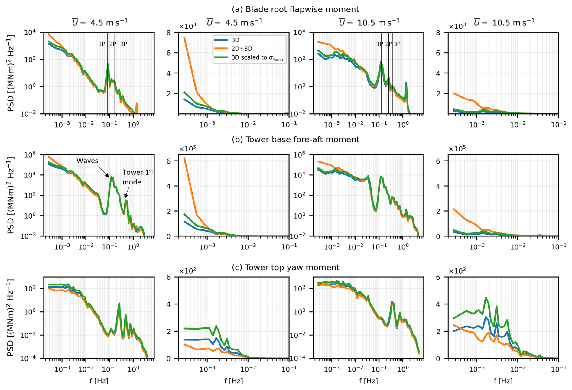
Figure 12 (a) Blade root flapwise moment, (b) tower base fore–aft moment, and (c) tower top yaw moment response of the floating IEA 15 MW wind turbine under different turbulent wind fields. These responses are shown for two wind speeds, i.e., 4.5 and 10.5 m s⁻¹. The first and third columns represent the full frequency range on a log–log plot, while the second and fourth columns zoom into the low frequencies. The vertical lines in the first row represent the 1P, 2P, and 3P frequencies of the rotor. In the tower base fore–aft moment, the waves and first tower mode are also indicated.

The tower base fore–aft moment presents a similar behavior as the blade root flapwise moment. In the full frequency range illustrated in Fig. 12b, a distinct peak corresponds to the wave-induced loading at around 0.13 Hz. It is worth noting that the first tower mode of the floating tower, i.e., approximately 0.48 Hz, falls outside the rotor's 1P–3P frequency range to avoid resonance. In the low-frequency response of the tower base fore–aft bending moment, the 2D turbulence has the highest response. At the lowest frequency analyzed in these plots, the tower base moment response to 2D turbulence is almost 3 times that of 3D turbulence.

The tower top yaw moment response for the IEA 15 MW floating configuration is illustrated in Fig. 12c. Interestingly, the tower top yaw response differs completely from the blade root flapwise and tower base fore–aft moments. Here, the response under 2D turbulence is also reduced at low frequencies. This can be attributed to the influence of large-scale coherent structures interacting with the turbine rotor, thereby decreasing torsional moments.

4.2.2 Floating platform translational motions

The translational motion response of the IEA 15 MW floating wind turbine platform to varying turbulent wind fields at two different wind speeds is displayed in Fig. 13. In the platform's surge response (Fig. 13a), two distinctive peaks corresponding to surge motion natural frequency and wave-induced motion are visible. In the low-frequency range, the impact of 2D turbulence is more pronounced at 4.5 m s⁻¹. At 10.5 m s⁻¹, the platform's surge frequency shows a stronger response than the low-frequency turbulent wind. In the case of the platform's sway motion exhibited in Fig. 13b, no significant response at the low frequencies was observed. The only observable peak in the PSD plot for the platform's sway motion corresponds to its natural frequency, i.e., 0.007 Hz. A significant increase in the response at this peak was observed as the wind speed increased from 4.5 to 10.5 m s⁻¹. The platform's heave motion, featured in Fig. 13c, is influenced by the wave field and its natural frequency at approximately 0.13 and 0.05 Hz, respectively. Although the platform's heave motion response is most pronounced at low frequencies under 2D turbulent wind, it did not exceed the responses at high frequencies due to wave-induced forces and the natural frequency.

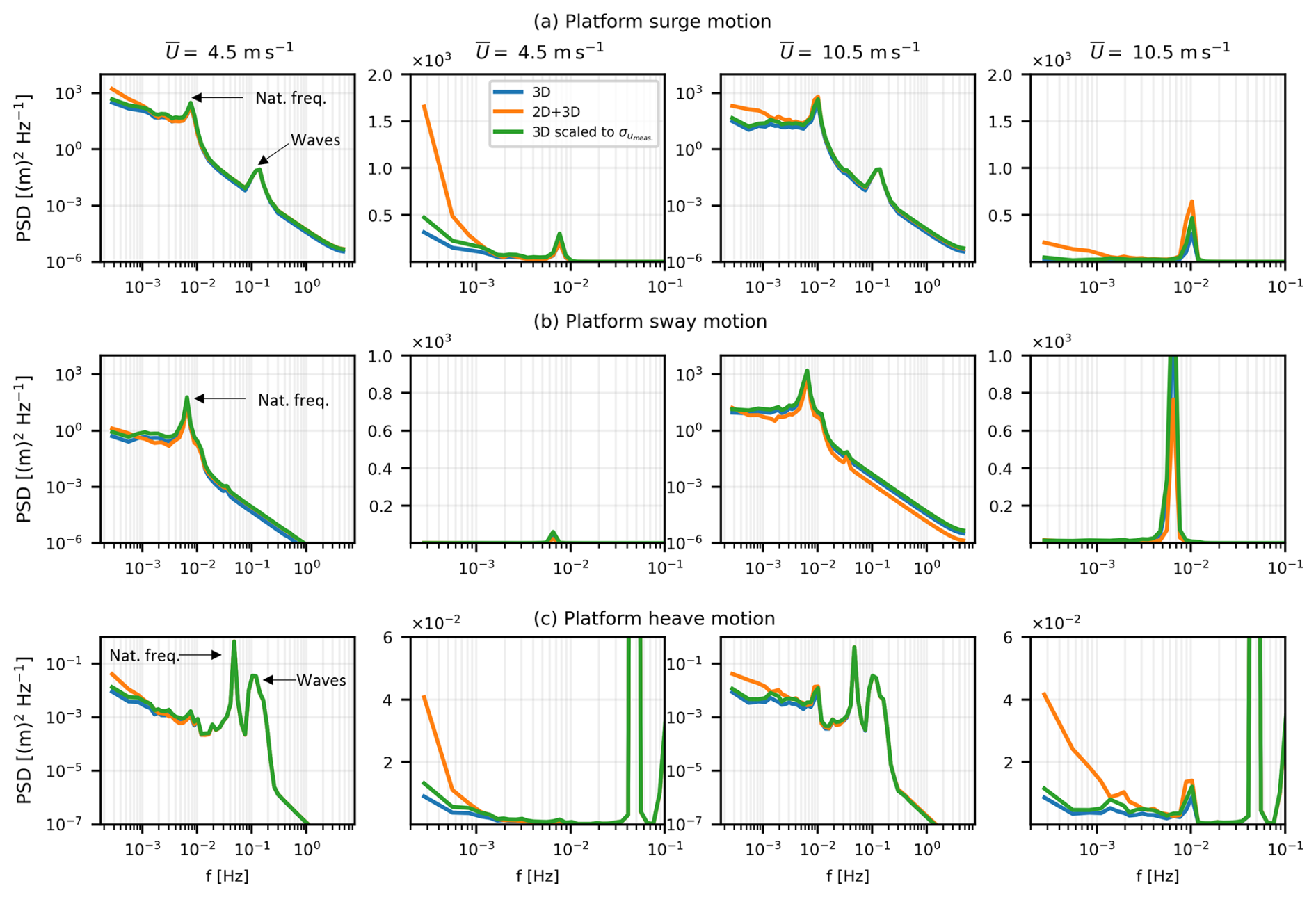
Figure 13 The response of the three translational motions, i.e., (a) surge, (b) sway, and (c) heave, of the semi-submersible platform to different wind fields. These responses are illustrated for two wind speeds, i.e., 4.5 and 10.5 m s⁻¹. The first and third columns represent the full frequency range on a log–log plot, while the second and fourth columns zoom into the low frequencies.

4.2.3 Floating platform rotational motions

Figure 14 provides an insight into the floating platform rotational motion response to different turbulent wind fields. The response is illustrated specifically for wind speeds 4.5 and 10.5 m s⁻¹. In the platform's roll motion (see Fig. 14a), the most prominent peak corresponds to the natural frequency of the roll motion. The PSD magnitude at all frequencies experiences a substantial increase as wind speed increases from 4.5 to 10.5 m s⁻¹. It is noted that the impact of 2D turbulence is insignificant compared to other sources of disturbance. The platform's pitch motion response, akin to the surge motion, is shown in Fig. 14b. Here, wave-induced pitch motion generates a pronounced peak at approximately 0.12 Hz. However, at low frequencies, 2D turbulence exhibits the highest response, with this response more pronounced at 4.5 m s⁻¹ than at 10.5 m s⁻¹. Regarding the platform's yaw motion, the low-frequency response is relatively subdued, as indicated in Fig. 14c. The most distinct peak in the platform's yaw response corresponds to the natural frequency of yaw motion, and it increases almost 6 times in magnitude when the wind speed is increased from 4.5 to 10.5 m s⁻¹.

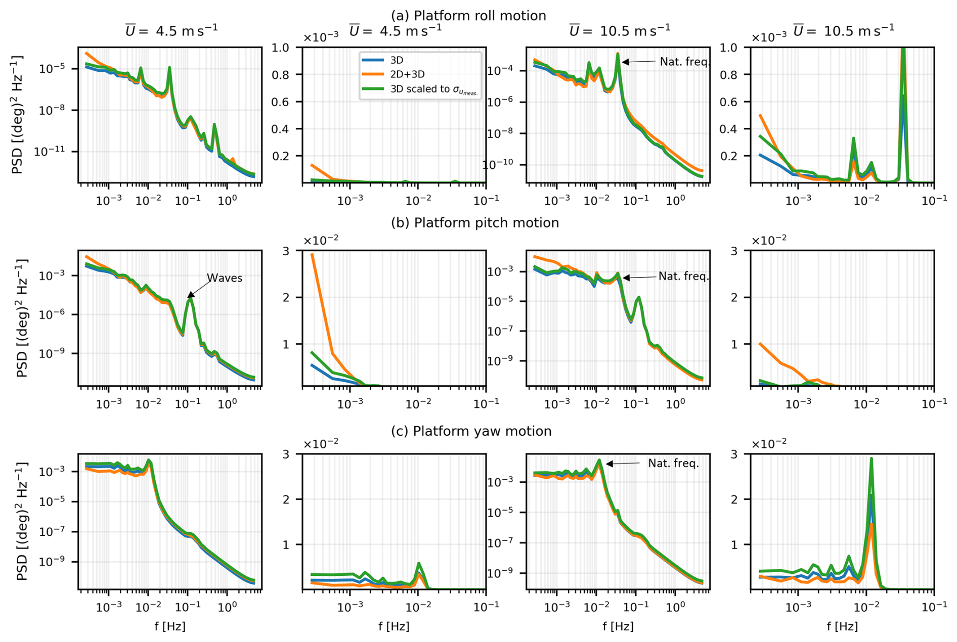
Figure 14 The response of the three rotational motions of the semi-submersible platform to different wind fields, i.e., (a) roll, (b) pitch, and (c) yaw. These responses are shown for two wind speeds, i.e., 4.5 and 10.5 m s⁻¹. The first and third columns represent the full frequency range on a log–log plot, while the second and fourth columns zoom into the low frequencies.

4.2.4 Mooring line tension

The three mooring lines are attached to the floating platform via fairleads (see Fig. 1b). Of the three mooring lines, only the response of the one directly facing the wind (windward) and waves is analyzed here, as it experiences the highest loading. The full frequency range response has several distinct peaks, as illustrated in Fig. 15. For instance, the excitation from the platform's surge motion natural frequency occurs at 0.007 Hz, while the peaks corresponding to waves and first tower mode are present at around 0.12 and 0.48 Hz, respectively. A few response peaks at frequencies exceeding 1 Hz are also observed, albeit with relatively smaller magnitudes. In the low-frequency region, it becomes evident that 2D turbulence significantly contributes to the heightened loading response, especially for frequencies below 10⁻³ Hz. Similar to the responses observed in the platform's surge motion and tower's fore–aft bending moment, the mooring line tension responses induced by all three turbulent wind fields decrease in magnitude at low frequencies with an increase in wind speed from 4.5 to 10.5 m s⁻¹. However, an increased response at approximately 0.009 Hz was observed at 10.5 m s⁻¹, which corresponds to the natural frequency of surge motion.

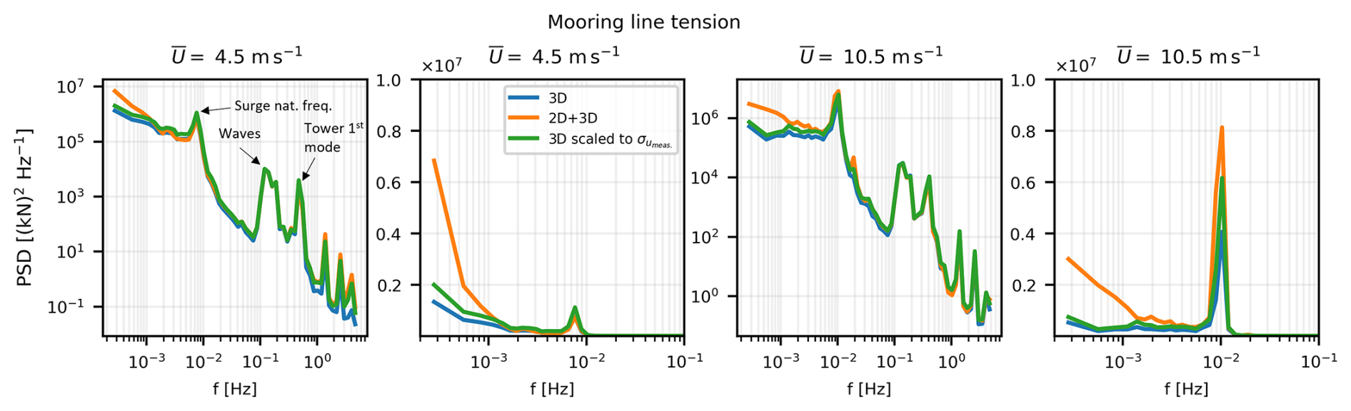
Figure 15 The response of the mooring line tension to different wind fields. These responses are shown for two wind speeds, i.e., 4.5 and 10.5 m s⁻¹. The first and third columns represent the full frequency range on a log–log plot, while the second and fourth columns zoom into the low frequencies. Peaks corresponding to surge, waves, and tower motion are also indicated.

5 Discussion

The presence of a large coherence in the longitudinal wind component (u) at frequencies below 10⁻³ Hz led to substantial tower base fore–aft and blade root out-of-plane bending moment loads for both fixed and floating wind turbines. The increase in DELs for these two moments was more pronounced at lower wind speeds, when the pitch regulation of the controller was not active. Furthermore, when the turbulent wind field consisted of 2D+3D turbulence, the load variation was more prominent for these moments. In contrast, the in-plane moments, namely the tower base side–side and blade root edgewise moments, decreased at higher wind speeds. The torsional moment, i.e., tower top yaw moment, decreased at all wind speeds in the 2D+3D turbulence case. This can be attributed to the presence of more coherent turbulence structures in the rotor plane in 2D turbulence, which leads to lower twisting moments.

Notably, tower fore–aft and blade root bending moments showed a stronger response at low frequencies for both fixed- and floating-turbine designs. These responses closely mirrored the wind spectra's behavior at low frequencies, indicating greater energy in low-frequency fluctuations at lower wind speeds than at higher wind speeds. In the case of platform motion responses in the floating wind turbine, surge and pitch displacements were most excited at low frequencies. These responses even exceeded the natural frequency excitation responses for surge and pitch motions at a wind speed of 4.5 m s⁻¹. Consequently, the fairlead tension of the windward mooring line increased significantly, more so at lower wind speeds and less so at higher wind speeds, when the platform's surge natural frequency became the dominant factor.

An interesting topic of investigation is whether systematic changes in the anisotropy (ψ) of 2D turbulence structures have any implications for DELs? The dominant drivers of thrust-induced loading on the tall wind turbines are primarily the variance (${\mathit{\sigma }}_{\text{2D}}^{\mathrm{2}}$) and the spatial coherence of the wind components (mainly u) across the rotor disk. The coherence is mainly governed by L_2D rather than the anisotropy ψ since for horizontal coherent structures with L_2D≫D_rotor (more than 500 times), the rotor is always embedded with a single eddy regardless of its horizontal shape. Oblate structures, where ψ<45°, would result in increased v fluctuations and thus a higher lateral coherence affecting side–side and yaw moments, and vice versa. However, these variations in ψ would have only a negligible effect on DEL due to the extremely large size of the structures in 2D turbulence. A dedicated sensitivity study of L_2D and ψ on DELs would be valuable and is recommended as future work, particularly because measurements at sites with stronger atmospheric stability stratification or in other marine environments may yield stronger anisotropy (Syed and Mann, 2024a).

The simulation setup utilized in this study deviates from the IEC standard in several aspects. The standard recommends specific values of the L_3D and Γ parameters of the Mann turbulence model. According to the standard, the length scale parameter L_3D=0.8Λ, where Λ is the turbulence scale parameter. For hub heights greater than 60 m, Λ=42 m, which suggests a length scale L_3D=29.4 m. The anisotropy parameter Γ is fixed at 3.9, and the energy dissipation parameter $\mathit{\alpha }{\mathit{ϵ}}^{\mathrm{2}/\mathrm{3}}$ is scaled to the target turbulence intensity (TI). These values are chosen to best match the Kaimal spectral model. However, Syed and Mann (2024a), Chougule et al. (2010), Sathe et al. (2013) have highlighted the strong dependence of these parameters on atmospheric stability. The use of these set parameters may not give the best match with measured spectra (also seen in Fig. 4). A consequence is an inaccurate estimation of the simulated loads and turbine responses. In this study, we used the parameters obtained by fitting the measured spectra to the Mann turbulence model.

Furthermore, the IEC standards recommend linear detrending of measured wind data before calculating the standard deviation of the longitudinal wind component. Dimitrov et al. (2017) noted that detrending causes the reduction in low-frequency content of a wind time series, resulting in reduced standard deviation. Although we applied criteria to remove extremely non-stationary time series (see Syed and Mann, 2024a), we did not apply linear detrending before evaluating the measured spectra. The resulting spectra have large energy in the u and v components at low frequencies, even though the time series were considered stationary. Typically, 10 min time series are used in design load case (DLC) studies, which the standard turbulence models capture very well, especially for onshore turbines. However, the low-frequency wind fluctuations important for offshore wind turbines are not observable in a short time series. Therefore, we used the 1 h time series to capture the low-frequency part of the wind spectrum as comprehensively as possible.

Finally, it is essential to note that the present study covers only the normal operating mode of the wind turbine and does not account for extreme turbulence events, such as ramp-like increases in wind speed associated with large-scale meteorological processes, as investigated by Hannesdóttir et al. (2019). The study presented here can be closely associated with DLC 1.2 in IEC standards, which focuses on evaluating fatigue loads from normal operation. The misalignment between wind and waves can also have a significant impact on the dynamic response of a floating offshore wind turbine, as investigated by Li et al. (2020). Here, we did not delve into this aspect since our primary focus was to examine the aerodynamic response to wind turbulence. A wind-speed-dependent wave climate would provide more representative DEL estimates and could also affect the dynamic response of the floating wind turbine, especially at higher wind speeds when wave loading may dominate wind loading. We acknowledge this limitation and recommend that future work incorporate wind-speed-dependent wave conditions in aeroelastic simulations to improve the reliability of the results.

6 Conclusions

This study investigates the impact of low-frequency wind turbulence on the damage equivalent loads and dynamic response of the IEA 15 MW reference wind turbine. A model for low-frequency anisotropic wind fluctuations was employed to simulate wind fields resembling those of the marine atmosphere. Low-frequency wind turbulence was combined with high-frequency wind turbulence simulated by the Mann uniform shear model to span a wide frequency range. The model parameters were obtained from 1 h spectra measurements at the FINO1 offshore research site in the North Sea. It was observed that the Mann turbulence model underestimated the flow turbulence at low frequencies, resulting in reduced standard deviation of the u and v wind components.

The response of the IEA 15 MW wind turbine was investigated under three different wind fields: (i) a 3D turbulent wind field that underestimates the u and v turbulence at low frequencies, (ii) a 2D+3D turbulent wind field that accurately models also the low-frequency wind fluctuations, and (iii) a scaled 3D turbulent field that mimics the 3D turbulent field but is scaled up to match the measured standard deviation of the u and v wind components. The simulations were performed using the HAWC2 aeroelastic code for each wind speed between the cut-in and cut-out wind speeds. Both fixed- and floating-turbine designs were considered.

Damage equivalent load (DEL) assessments were performed for five moments: tower base fore–aft, tower base side–side, tower top yaw, blade root flapwise, and blade root edgewise moments. The scaled 3D turbulence resulted in the highest DEL for all five moments, indicating a greater impact of high-frequency turbulence on DEL than low-frequency turbulence. Compared with the unscaled 3D turbulence, the highest DELs were observed for the tower fore–aft and blade root flapwise moments at low wind speeds with the 2D+3D turbulence model. We observed strong coherence in the longitudinal wind component at low frequencies in the wind fields simulated by the 2D+3D turbulence model. This also resulted in reduced torsional moments acting on the rotor, as evidenced by the lower DEL values at the tower top yaw moment in this case. A similar trend was observed in the floating wind turbine, except that the magnitude of DEL for tower moments was almost twice as large due to a different tower design.

The dynamic response of the moments due to longitudinal forces showed behavior similar to that of the wind spectra. This includes the tower fore–aft and blade root flapwise moments. A heightened response of these moments was observed for frequencies below $\mathrm{2}\times {\mathrm{10}}^{-\mathrm{3}}$ Hz in the case of 2D+3D turbulence. However, this response was less pronounced at high wind speeds than at low wind speeds. Additionally, the rigid-body motion response of the floating platform was investigated in this study. It was observed that out of the six floating platform motions, only surge and pitch motions significantly responded to 2D turbulence. At a low wind speed of 4.5 m s⁻¹, both surge and pitch motion showed a pronounced response to low-frequency wind turbulence. This response was attenuated at 10.5 m s⁻¹, and in the case of the surge motion, the natural frequency response overshadowed it. Furthermore, the fairlead tension in the windward mooring line also increased at low frequencies in response to 2D+3D turbulence.

These results show that for large offshore wind turbines, the effect of low-frequency wind fluctuations can not be ignored. This study demonstrates the importance of accurately simulating low-frequency wind fluctuations to effectively assess the wind turbine's response.