Lifetime reassessment of offshore wind turbines considering different operating conditions using Kriging meta-models

To extend the lifetime of an offshore wind turbine, a lifetime reassessment is required to determine the potential remaining lifetime. This means that the lifetime is recalculated using the combinations of environmental parameters (wind and wave effects) that have actually occurred during the lifetime and which typically differ from the assumed conditions during design. The computational effort of such a lifetime reassessment is significant, as a very large number of aeroelastic simulations have to be carried out. Therefore, according to the state of the art, the number of considered combinations of environmental parameters is reduced similar to the design procedure. In this work, an alternative approach for the lifetime reassessment is investigated in detail. This retains the full set of combinations of environmental parameters while considering both normal operation and idling. The challenge of the high computational effort is resolved by using Kriging meta-models instead of aeroelastic simulations. The meta-model-based approach is compared to two other methods for lifetime reassessment: first, the reference method, i.e. a full lifetime reassessment using aeroelastic simulations where all combinations of environmental parameters which have actually occurred are considered, and second, the approach according to IEC 61400-3. The three methods are compared with regard to the accuracy of their overall lifetime predictions and the computational effort required to make the lifetime predictions. The results show that both the IEC approach and the meta-model approach can achieve good lifetime prediction accuracy compared with the reference method. However, compared to the reference solution, whilst the IEC-based approach can reduce the computational effort to approximately 20 % of the reference solution's computational effort, the use of meta-models can significantly reduce it to less than 0.5 % of the reference solution's computational effort. The results therefore show that, by using meta-models instead of the original aeroelastic simulation model to reassess the lifetime, the computational effort can be significantly reduced compared to the other two methods, while maintaining a high approximation quality in the prediction of the lifetime fatigue loads.

1 Introduction

Offshore wind turbines are usually designed for a lifetime of 25 years. After this period, there are various options regarding further use of the wind turbines, e.g. decommissioning, re-powering, or lifetime extension. In the case of lifetime extension, the wind turbine is kept in operation beyond its originally intended lifetime. However, to extend the lifetime, the remaining safe lifetime of the wind turbine must first be determined. This can be done using a lifetime reassessment or recalculation. Here, the lifetime is recalculated using the environmental conditions (wind and wave effects) that have actually occurred during the lifetime. However, this means that a large number of combinations of environmental parameters, which demand aeroelastic simulations, must be taken into account. Due to the resulting large number of simulations required (approximately 1 000 000 simulations), it is hardly possible to perform an exact lifetime reassessment using an aeroelastic simulation model.

One option for significantly reducing the calculation effort is to reduce the number of considered combinations of environmental conditions. This is the approach recommended by the standards (IEC 61400-1; IEC, 2019a and IEC 61400-3; IEC, 2019b) and was carried out by Stewart (2016), Ziegler and Muskulus (2016), Bouty et al. (2017), Velarde et al. (2020), and Katsikogiannis et al. (2021). However, this method does not take into account all combinations of environmental parameters that may have occurred, so that the combination of this and the extrapolation to the lifetime using the probability of occurrence of each input parameter creates uncertainty in the prediction of the lifetime.

An alternative to a reduction in input parameter combinations is the use of meta-models as surrogates of the original aeroelastic simulation model. Due to the significantly reduced computing time of meta-models, all combinations of environmental parameters that have actually occurred can be calculated, although each calculation is only an approximation compared to the original aeroelastic simulation model. Due to the low computing time of the meta-models, another advantage of using meta-models is that changes during the lifetime of the wind turbine can be taken into account quickly. For example, the lifetime may need to be calculated several times because a new wind farm has been built nearby during the lifetime, which changes the wind conditions in the existing wind farm. Another reason could be an adjustment of the control strategy of the wind turbine during its lifetime. In these cases, if a meta-model is used, only a new calculation with the meta-model is necessary or (in the latter case) a new meta-model needs to be created. In contrast, without a meta-model, it is not possible to re-simulate the complete lifetime with the original simulation model due to the large number of required simulations.

Meta-models or surrogate models for fatigue load prediction, such as Kriging or Gaussian process regression (e.g. Dimitrov et al., 2018, Slot et al., 2020, Wilkie, 2020, Avendaño-Valencia et al., 2021, Müller et al., 2022, Singh et al., 2024), artificial neural networks (ANNs; e.g. Müller et al., 2017, 2021, Schröder et al., 2018, Haghi and Crawford, 2024), polynomial chaos expanson (PCE; e.g. Dimitrov et al., 2018, Murcia, 2018, Schröder et al., 2018, Slot et al., 2020), or mixture density networks (e.g. Singh et al., 2024, Singh et al., 2025), have been comprehensively investigated in recent years for operating conditions experienced by both onshore and offshore wind turbines. This has involved both more detailed investigations of meta-models and comparative studies (e.g. Dimitrov et al., 2018, Schröder et al., 2018, Slot et al., 2020, Müller et al., 2021, Singh et al., 2024) in which several meta-models were compared with each other. For idling conditions, the use of meta-models for predicting fatigue loads was recently investigated by Schmidt et al. (2025a). In all these studies, it turned out that the use of meta-models for both onshore and offshore wind turbines offers a good approach, regardless of the operating status of the wind turbine, to calculating fatigue loads with a feasible computational effort compared to the use of the original aeroelastic simulation model.

However, there are only a few studies in which the lifetime of wind turbines has been calculated using meta-models and compared with other methods for the lifetime calculation. For example, Stewart (2016) investigated different methods to reduce the simulation size for the lifetime calculation of a floating wind turbine. Among other things, the author investigated the use of response surface methods and genetic programming. These results were compared with lifetime damage equivalent loads (DELs), which were calculated from about 30 000 aeroelastic simulations. It turned out that the utilised response surface method is not able to capture all the important effects for predicting fatigue loads, while genetic programming led to good results. Dimitrov et al. (2018) compared the predicted lifetime DELs of an onshore wind turbine using five different meta-models, with the lifetime DELs determined using 1000 aeroelastic simulations created with a quasi Monte Carlo sampling for seven different reference sites plus the standard reference classes from IEC 61400-1 (IEC, 2019a). The results show that the PCE and Kriging approaches both show a good accuracy in prediction of the site-specific lifetime DELs, with Kriging being slightly more accurate but requiring more computing time. Schmidt et al. (2023) conducted a lifetime reassessment for an offshore wind turbine using Kriging meta-models considering 100 000 input parameter combinations which correspond to approximately 1.9 years and compared this to the results of aeroelastic simulations using the same 100 000 input parameter combinations. Additionally, a comparison with the approach according to IEC 61400-3 (IEC, 2019b) was performed. It turned out that the utilised Kriging meta-models are suitable for conducting a lifetime reassessment compared to the other two methods, as a high degree of accuracy and a low computational effort can be achieved by using the meta-models instead of the aeroelastic simulations. All mentioned studies have in common that only normal operation was investigated. However, according to IEC 61400-1 (IEC, 2019a), in addition to normal operation, idling must also be taken into account when calculating the lifetime of an (offshore) wind turbine. To the authors' knowledge, a lifetime reassessment using meta-models considering different operating conditions (e.g. normal operation and idling) has not yet been investigated. Furthermore, although the numbers of considered simulations in the different studies are in some cases very high, they remain well below the number of input parameter combinations that will affect an (offshore) wind turbine over its 20- to 25-year lifetime. These two gaps in literature regarding lifetime reassessment of (offshore) wind turbines using meta-models – namely, the absence of considering idling conditions and the absence of considering the entire lifetime – will be addressed in this paper.

For this reason, in this study, a lifetime reassessment is performed using Kriging meta-models, taking into account the entire lifetime of the wind turbine and considering not only normal operation but also idling conditions. This lifetime calculation is then compared with the results of two other methods for calculating the lifetime, which use aeroelastic simulations. First, a full lifetime calculation, where the same input parameter combinations were used to calculate the lifetime as for the meta-model-based method. And second, a lifetime calculation according to the standard IEC 61400-3 (IEC, 2019b). The aim is to find out to what extent the Kriging meta-models are suitable for the lifetime calculation compared to other methods and to identify the differences between the three methods. It should be mentioned that all considered methods can be used both for the design of an offshore wind turbine and for the lifetime reassessment. In the following, the terms lifetime reassessment and lifetime calculation are used.

The paper is structured as follows. First, in Sect. 2, the three methods for lifetime reassessment are detailed. In Sect. 3, in a first study, the three different methods for lifetime reassessment are compared. Among other things, this involves investigating how much computational effort the individual methods require for the lifetime calculation. In a second study (Sect. 4), the impact of the wind turbine availability on the lifetime DELs is investigated. At the end (Sect. 5), a conclusion is drawn.

2 Method

2.1 Simulation model and settings for the aeroelastic simulation model

The time-domain simulations for the investigations in this work are conducted using the aero-hydro-servo-elastic code FASTv8 from the National Renewable Energy Laboratory (Jonkman, 2013). The FASTv8 code was enhanced by introducing soil–structure interactions (Häfele et al., 2016; Hübler et al., 2018). As the wind turbine model, the NREL 5 MW reference wind turbine (Jonkman et al., 2009) with the OC3 monopile and soil (Jonkman and Musial, 2010) is used. As proceeded in Hübler et al. (2017a, 2018), the required soil matrices for the soil model are based on the lateral soil model of Kallehave (2012) and on the axial soil model of FUGRO (API, 2007). Initial conditions were used for the calculation of the soil matrices in accordance with Häfele et al. (2016), i.e. no loads were applied.

The turbulent wind field is calculated using TurbSim (Jonkman, 2016). Here, the Kaimal turbulence model is used, which is one of the turbulence models recommended in the IEC 61400-1 standard (IEC, 2019a) and which is frequently used, for example, by Yang et al. (2015), Slot et al. (2020), and Wilkie (2020). The irregular waves are calculated using the JONSWAP spectrum. The JONSWAP spectrum is commonly used for offshore wind turbine simulations, e.g. by Velarde et al. (2019), Stieng and Muskulus (2020), and Wilkie (2020).

The simulation length of each simulation is 10 min. In addition, a run-in time is included, which is cut off to remove the influence of the initial transients resulting from the abrupt loading at the beginning of the simulation. As previously mentioned, the simulations in the time domain are carried out both for normal operation and idling. Due to the different structural behaviour of the wind turbine during normal operation and idling, caused by the lower aerodynamic damping and an associated greater impact of the wave loads for the idling wind turbine, different run-in times must be taken into account for the two operating states (Schmidt et al., 2025a). For normal operation, a 240 s run-in time is used in this work. According to Hübler et al. (2017b), this additional simulation time should be sufficient for the calculation of fatigue loads for the NREL 5 MW reference turbine on a monopile for normal operation. For idling, run-in times between 60 and 800 s are chosen depending on the wind speed according to Schmidt et al. (2025a).

Five scattering environmental parameters (mean wind speed v_s, turbulence intensity TI, significant wave height H_s, wave peak period T_p, and wind–wave misalignment θ_mis) are considered in this work. Hübler et al. (2017a), Murcia (2018), and Velarde et al. (2019) identified these parameters as significant in sensitivity analyses for operating wind turbines. Due to their significant impact on the fatigue loads of operating wind turbines, it is assumed that these parameters also have a significant influence on the fatigue loads of an idling wind turbine. Additionally, for idling load cases, the initial rotor position ψ (azimuth angle) is considered a scattering parameter. In an earlier study (Schmidt et al., 2025a), it was found that for idling wind turbines, the variation in this parameter is relevant for determining the fatigue loads at the rotor blade root. For the five environmental parameters mentioned, the statistical distributions by Hübler et al. (2017b) are used, which were fitted against the measured environmental conditions at the FINO 3 research platform in the German North Sea. For ψ, for each input parameter combination, a random value between 0 and 360° is chosen.

The simulated loads in the time domain are transformed into short-term DELs according to the Palmgren–Miner rule. The short-term DELs are calculated as follows:

$$\begin{array}{}\text{(1)}& S_{\text{eq}}={\left(\sum {\displaystyle \frac{n_i{S}_i^m}{N_{\text{ref}}}}\right)}^{\frac{\mathrm{1}}{m}}.\end{array}$$

Here, n_i is the corresponding number of cycles for each load amplitude S_i determined by rainflow counting according to the standard ASTM E1049-85 (ASTM, 2017). N_ref=600 is the number of equivalent cycles for a frequency of 1 Hz for a 10 min time series and m is the Wöhler exponent. The Wöhler exponent m=3 is chosen for steel and m=10 for the composite material of the rotor blade. The load amplitude S_i is corrected according to Goodman (1914).

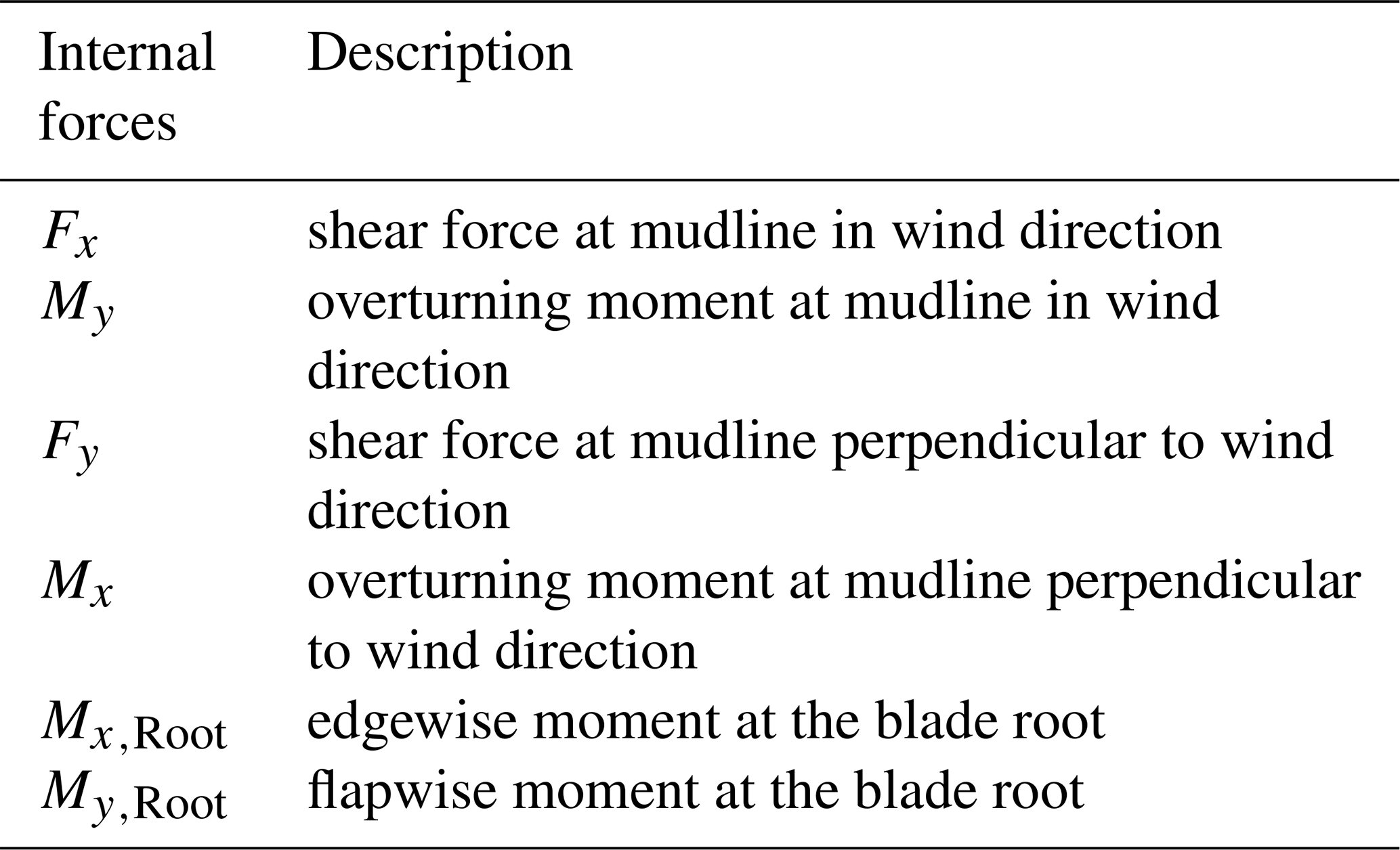
The lifetime reassessment in this work is carried out for the internal forces at the base of the monopile and at the rotor blade root. A visualisation of the considered locations and a list of the internal forces can be found in Fig. 1 and Table 1, respectively.

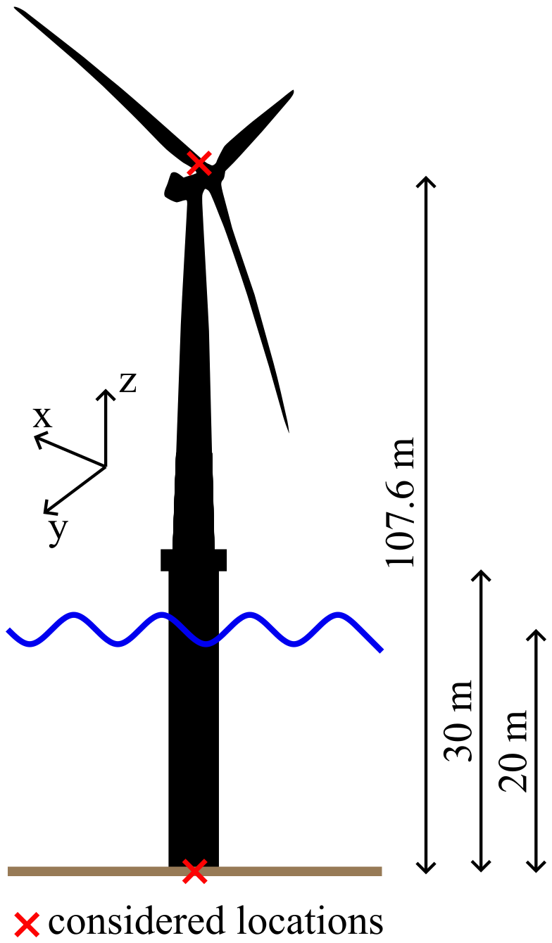
Figure 1 Visualisation of the NREL 5 MW reference turbine on the OC3 monopile (not to scale) with markings indicating the locations at which the internal forces are determined.

Table 1 Internal forces considered for the lifetime reassessment.

2.2 Kriging meta-models

In this work, Kriging meta-models are used for the lifetime reassessment of an offshore wind turbine. Kriging, also known as Gaussian process regression, is chosen because it has shown promising results in previous work, in terms of both approximation quality and computational effort required to create the meta-models (Slot et al., 2020; Wilkie, 2020). Furthermore, for the offshore wind turbine considered in this study (NREL 5 MW reference wind turbine on the OC3 monopile), Kriging meta-models already exist for normal operation and idling conditions (Müller et al., 2022; Schmidt et al., 2025a) so that these can be easily used.

Kriging combines a regression equation to model the mean or general trend in the data and a Gaussian process (GP) with a zero mean to model the deviations from the general trend (Santner et al., 2018). The mathematical equation is composed as follows (Rasmussen and Williams, 2006):

$$\begin{array}{}\text{(2)}& g\left(\mathbf{x}\right)=f\left(\mathbf{x}\right)+\mathbf{h}(\mathbf{x}{)}^{\mathrm{T}}\mathit{\beta }.\end{array}$$

Here, h(x)^Tβ represents the general trend in the data with known regression or basis functions h(x) and unknown regression coefficients β. f(x) is a Gaussian process with a zero mean and the covariance function or kernel function $k(\mathbf{x},{\mathbf{x}}^{\prime })$:

$$\begin{array}{}\text{(3)}& f\left(\mathbf{x}\right)\sim \text{GP}(\mathrm{0},k(\mathbf{x},{\mathbf{x}}^{\prime }\left)\right).\end{array}$$

As mentioned before, by using the Gaussian process, the deviations from the general trend, which are also called residuals, are modelled. The covariance function $k(\mathbf{x},{\mathbf{x}}^{\prime })$ describes the similarity between different data points (x and x^′). Here, it is assumed that data points whose input values are close to each other, i.e. are similar, also have similar output values. The covariance functions used can be isotropic or anisotropic. While isotropic covariance functions use the same correlation length for each input parameter, anisotropic covariance functions use a separate correlation length for each input parameter. For more information on Kriging, the reader is referred to Santner et al. (2018) and Rasmussen and Williams (2006).

The Kriging meta-models used in this work are surrogate models of the offshore wind turbine described in Sect. 2.1. The Kriging meta-models are used to predict the short-term DELs S_eq as defined in Eq. (1) for the internal forces summarised in Table 1. For normal operation and idling, separate meta-models from previous works (Müller et al., 2022; Schmidt et al., 2025a) are used or newly created based on the findings in the aforementioned works.

In normal operation, for the internal forces and moments at the monopile, the Kriging meta-models investigated in Müller et al. (2022) are used. The meta-models are trained using a pure quadratic basis function and the anisotropic Matérn $\mathrm{3}/\mathrm{2}$ covariance function. Since the current study aims to recalculate the lifetime for the edgewise and flapwise bending moments at the rotor blade root, but Müller et al. (2022) only investigated in-plane and out-of-plane bending moments, the meta-models for the edgewise and flapwise bending moments are created in the same way as described in Müller et al. (2022) for the in-plane and out-of-plane bending moments. For idling, the Kriging meta-models created by Schmidt et al. (2025a) are used. These were trained using a linear basis function and the anisotropic Matérn 3$/$2 covariance function.

The input parameters of the meta-models are the five environmental parameters mentioned previously in Sect. 2.1 (v_s, TI, H_s, T_p, θ_mis). In addition, as described in Schmidt et al. (2025a), for the rotor blades under idling conditions, ψ and the mean rotor speed ω are taken into account as additional input parameters. All meta-models used were created with 8500 training samples, and an additional 1500 test samples were used to test the meta-models. The training and test samples were created using Halton sequences and the statistical distributions of Hübler et al. (2017b) referring to the FINO 3 research platform. For more information regarding the utilised Kriging meta-models, the reader is referred to Müller et al. (2022) and Schmidt et al. (2025a).

Kriging meta-models generally predict a mean and a corresponding standard deviation for each short-term DEL. For the prediction of the short-term DELs in this work, only the predicted mean values are used.

2.3 Lifetime reassessment

In this work, three different methods for a lifetime reassessment of offshore wind turbines are investigated and compared. The first method is a full lifetime reassessment using aeroelastic simulations. This method represents an accurate lifetime calculation and is therefore used as a reference solution within the scope of this work. The second method is a lifetime reassessment according to IEC 61400-3 and the third method is a lifetime reassessment using Kriging meta-models. The three methods are compared to identify differences and to find out whether the use of meta-models is suitable for a lifetime reassessment of offshore wind turbines. In the following, the three methods are discussed more in detail.

2.3.1 Full lifetime reassessment

For the full lifetime reassessment, i.e. the reference solution, aeroelastic simulations are carried out using the simulation model and settings described in Sect. 2.1. As described in Sect. 2.1, both normal operation and idling are considered. Idling is taken into account for wind speeds outside the wind speed range of normal operation ($v_{\mathrm{s}}<\mathrm{3}\mathrm{m}{\mathrm{s}}^{-\mathrm{1}}$ and $v_{\mathrm{s}}>\mathrm{25}\mathrm{m}{\mathrm{s}}^{-\mathrm{1}}$). In addition, an availability of the wind turbine of 90 % is assumed in accordance with IEC 61400-3 (IEC, 2019b). This means that 10 % of all occurring load cases during the lifetime of the wind turbine are idling load cases due to the non-availability of the wind turbine. These 10 % are assumed to be independent of the wind speed. The lifetime reassessment is therefore divided into two cases: the wind turbine is available, i.e. normal operation for $\mathrm{3}\mathrm{m}{\mathrm{s}}^{-\mathrm{1}}\le v_{\mathrm{s}}\le \mathrm{25}\mathrm{m}{\mathrm{s}}^{-\mathrm{1}}$ and idling for $v_{\mathrm{s}}<\mathrm{3}\mathrm{m}{\mathrm{s}}^{-\mathrm{1}}$ and $v_{\mathrm{s}}>\mathrm{25}\mathrm{m}{\mathrm{s}}^{-\mathrm{1}}$, and the case where the wind turbine is not available, i.e. idling across the entire wind speed range.

The input parameter combinations for the aeroelastic simulations are created with the help of the Monte Carlo method using the statistical distributions referring to the environmental parameters of the FINO 3 research platform from Hübler et al. (2017b). According to Dimitrov et al. (2018), the resulting short-term DELs from the aeroelastic simulations are then converted into lifetime DELs using the following equation:

$$\begin{array}{}\text{(4)}& S_{\text{eq,lifetime}}={\left[\sum _{i=\mathrm{1}}^N{\left[S_{\text{eq}}\left({\mathit{x}}_i\right)\right]}^{m}p\left({\mathit{x}}_i\right)\right]}^{\frac{\mathrm{1}}{m}}.\end{array}$$

Here, x_i is the ith vector of input variables. Under both normal operation and idling, for the internal forces and moments at the monopile, x_i=[v_s TI H_s T_p θ_mis]^T and when idling, for the rotor blades, x_i=[v_s TI H_s T_p θ_mis ψ]^T. N is the number of simulations and p(x_i) is the probability of occurrence of each simulation. Here, due to the Monte Carlo sampling, the probability of occurrence of each simulation is $p\left({\mathit{x}}_i\right)=\mathrm{1}/N$. A separate lifetime DEL is calculated for each of the two cases “wind turbine is available” and “wind turbine is not available”. These are then weighted and added together as shown in Eq. (5).

$$\begin{array}{}\text{(5)}& \begin{array}{rl}{\displaystyle }{S}_{\text{eq,lifetime,total}}& {\displaystyle }=\left(S_{\text{eq,lifetime,avail}}^m\times p_{\text{avail}}\right.\\ {\displaystyle }& {\displaystyle }{\left.+S_{\text{eq,lifetime,unavail}}^m\times p_{\text{unavail}}\right)}^{\frac{\mathrm{1}}{m}}\end{array}\end{array}$$

The case of the available wind turbine is weighted with p_avail=0.9 and the case of the unavailable wind turbine with p_unavail=0.1.

To consider the complete lifetime of 25 years, performing 1 314 900 10 min simulations would be necessary. However, as previously mentioned, the simulations are sampled from probability distributions of the environmental parameters using the Monte Carlo method. Therefore, it must first be determined whether it is necessary to simulate the entire 25 years or whether the lifetime DELs may already converge with fewer simulations. To analyse this, the number of simulations used to calculate the lifetime DELs is increased step by step. As described above, a distinction is made during the investigation as to whether the wind turbine is generally available (combination of normal operation and idling load cases, 90 % of the lifetime) or whether the wind turbine is not available (only idling load cases for all wind speeds, 10 % of the lifetime). Based on this categorisation, the maximum number of simulations for the available case is 1 183 410, and for the unavailable case 131 490. For the convergence studies, initially, 440 000 simulations are performed for the case where the wind turbine is available, which corresponds to approximately one-third of the total number of simulations of 1 314 900. For the convergence study of the unavailable wind turbine, however, only 150 000 simulations are performed, as the total number for this case is already 131 490 simulations and therefore no further simulations are required.

The results are shown in Fig. 2a for the available wind turbine and in Fig. 2b for the unavailable wind turbine. The lifetime DELs are normalised for each internal force using the lifetime DELs for the maximum number of simulations investigated (440 000 for the available case, 150 000 for the unavailable case). Convergence is assumed if the deviation of the corresponding lifetime DEL is less than 0.5 % compared to the lifetime DEL determined with the maximum number of simulations investigated. It is assumed that with a convergence criterion of a maximum deviation of 0.5 %, a level of accuracy has been achieved which is, in any case, lower than other uncertainties arising within the calculations of the lifetime DELs.

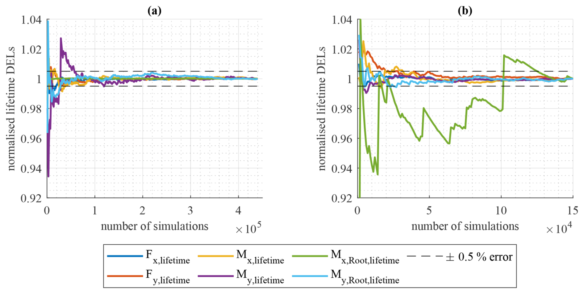
Figure 2 Normalised lifetime DELs of the reference solution depending on the number of simulations. (a) Wind turbine is available (normal operation and idling conditions for wind speeds outside the wind speed range of normal operation); (b) wind turbine is not available (only idling). The lifetime DELs are normalised using the lifetime DELs determined with the maximum number of simulations.

From Fig. 2, it becomes clear that, for the available case, the normalised lifetime DELs for each of the internal forces investigated converge after just over 100 000 simulations. For the unavailable wind turbine, the normalised lifetime DELs converge after less than 100 000 simulations, except for M_{x,Root,lifetime}. The convergence behaviour of M_{x,Root,lifetime}, however, is significantly worse. The curve shows clear jumps, even with a comparatively high number of simulations around 100 000. These jumps are caused by some few simulations in which the wave peak period has values of approximately 4 or 8 s and the resulting short-term DELs of M_x,Root are very large. One possible explanation for these large values of the resulting short-term DELs is that in these simulations, the wind turbine is excited at its natural frequency, causing the rotor blades to vibrate strongly, which is why the short-term DELs have very high values. To investigate whether these outliers only occur for very specific wind and wave conditions that might not even occur in reality (i.e. numerical artefacts in the aeroelastic code), the corresponding simulations are performed again with changed wind and wave seeds (all other input parameters are kept unchanged). The results for M_{x,Root,lifetime} with changed wind and wave seeds for the outliers are shown in Fig. 3 together with the original curve of M_{x,Root,lifetime} from Fig. 2b. It becomes clear that only by changing the random seeds in the corresponding few simulations that previously predicted very large short-term DELs can the convergence behaviour be significantly improved. This leads to the conclusion that, in these few simulations, it is not the combination of input parameters itself but rather the combination of the input parameters in conjunction with the random seeds that can, in some rare cases, lead to very high short-term DELs due to the strong vibration of the wind turbine. It is assumed that this strong oscillation of the wind turbine rotor blades does not occur in reality but is rather an effect of FASTv8 resulting from the simplified modelling of the wind turbine. However, it is still the case that the lifetime DEL of M_x,Root with the changed random seeds only shows a deviation of less than 0.5 % from the lifetime DEL determined with 150 000 simulations when using approximately 130 000 simulations. For this reason, in the further course of the work, the lifetime DELs for the unavailable wind turbine are determined using the maximum number of 131 490 simulations. For the available wind turbine, 200 000 simulations are chosen to be on the safe side as the lifetime DELs converge better using 200 000 simulations instead of 100 000 simulations.

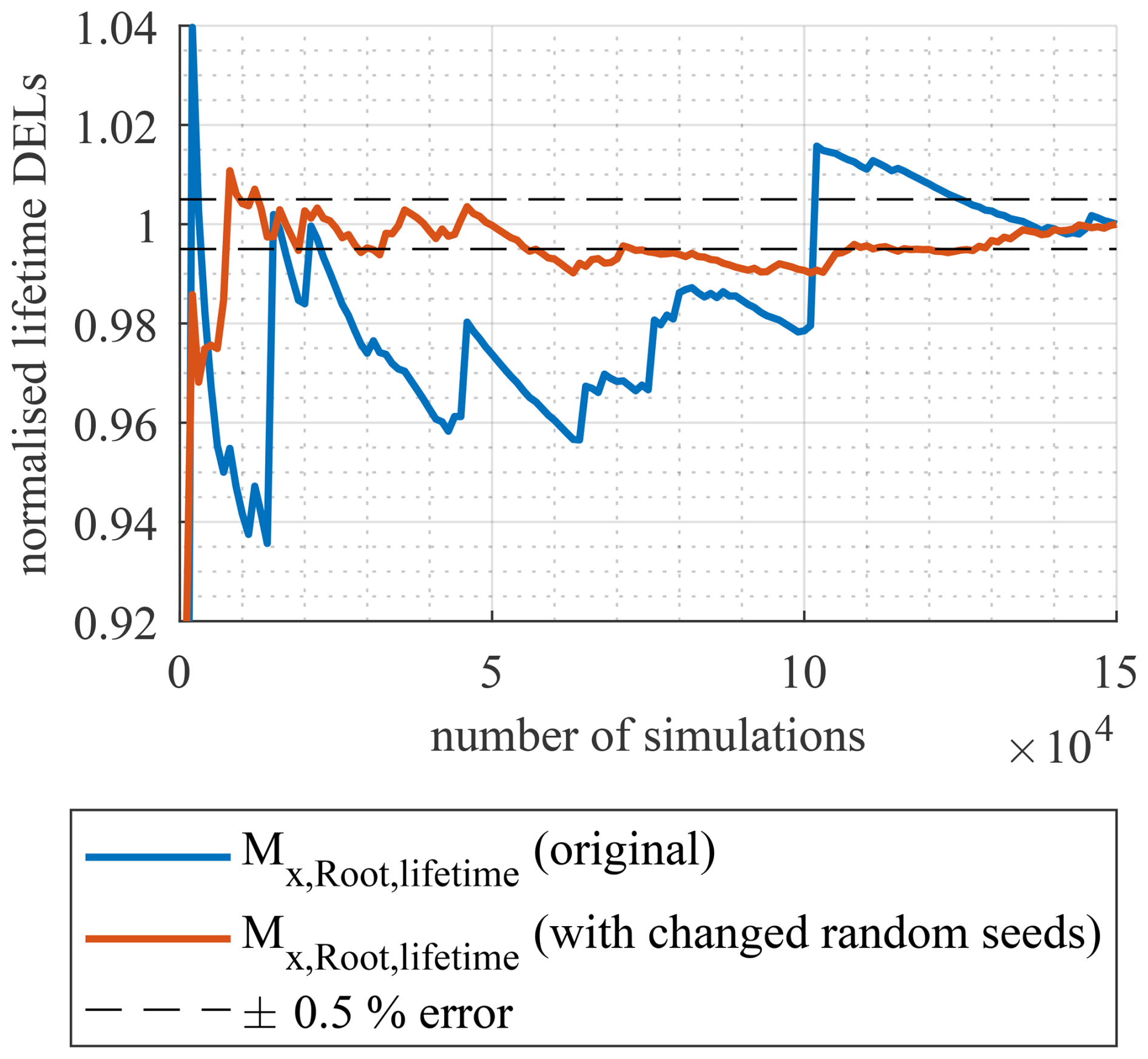
Figure 3 Normalised lifetime DELs of the reference solution of M_x,Root depending on the number of simulations for the unavailable wind turbine. Comparison of original curve from Fig. 2b with curve created using changed random seeds for the outliers. The lifetime DELs are normalised using the lifetime DELs determined with the maximum number of simulations.

2.3.2 Lifetime reassessment according to the standard IEC 61400-3

For the lifetime reassessment according to the standard IEC 61400-3 (IEC, 2019b), the input parameters v_s, H_s, and T_p must be considered to be scattering parameters. Additionally, the wind and wave directions can be taken into account. In this work, the wind–wave misalignment θ_mis is considered instead. This is consistent with the work of Stewart (2016) and with our previous work (Schmidt et al., 2023). According to IEC 61400-1 (IEC, 2019a), the 90th percentile of the corresponding probability distribution should be used for TI. Since the use of the 90th percentile for TI can lead to significantly higher lifetime DELs compared to the other methods used in this work, where TI is considered a scattering parameter (Schmidt et al., 2023), instead of the 90th percentile for TI, in this study, the mean value for TI is employed.

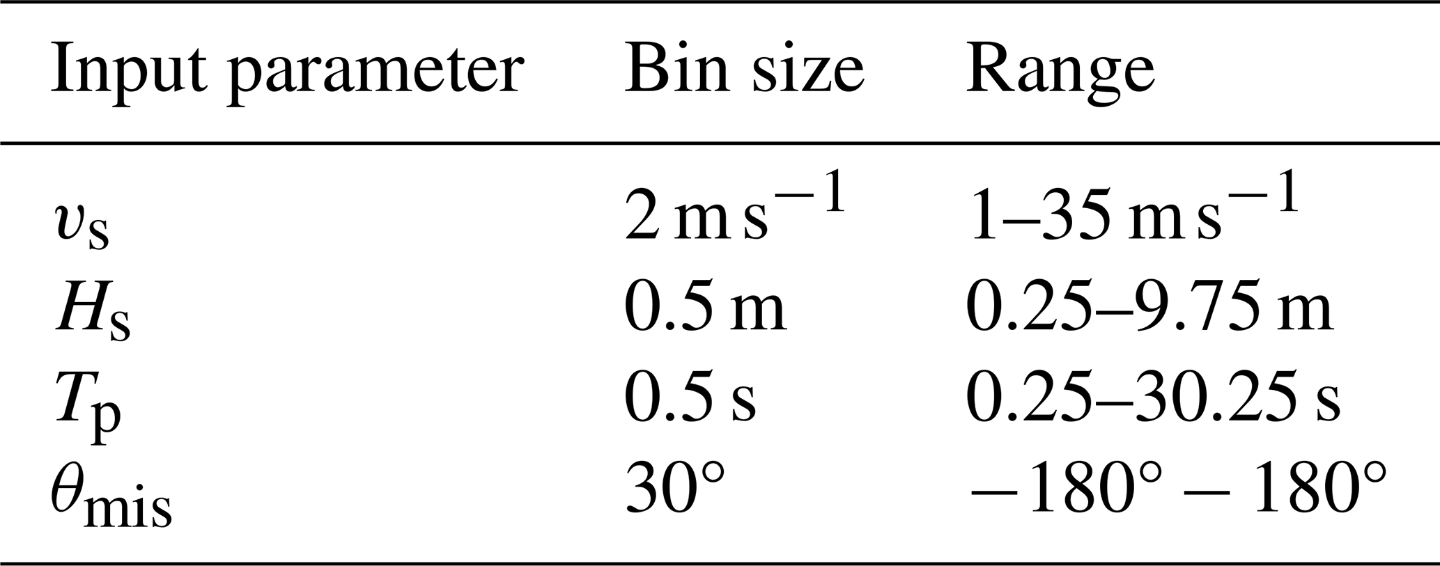
To create the load case set, the probability distributions of the four input parameters are divided according to the bin sizes given in Table 2. For each bin of each input parameter, the probability of occurrence is determined. Then all possible combinations of the four input parameters are determined, and for each input parameter combination, the probability of occurrence is calculated by multiplying the probabilities of occurrence of each of the four parameters. If all possible combinations of the four input parameters are considered, for the statistical distributions referring to the FINO 3 research platform (Hübler et al., 2017b), this results in 263 520 simulations. Additionally, according to IEC 61400-3, six 10 min simulations with different seeds or one 1 h simulation must be carried out. In the case of six different seeds, this results in a number of 1 581 120 simulations.

Table 2 Considered bin sizes according to IEC 61400-3 and ranges of the input parameters.

The computational effort needed to conduct these number of simulations is very high. However, by taking into account all possible combinations of the input parameters, combinations are also considered that do not or only very rarely occur in reality, such as a low wave height in combination with a high wind speed. To reduce the computing time, combinations with a very low probability of occurrence are therefore not considered. For these load cases, it can be assumed that the probability of occurrence of these load cases is so small that the impact on the lifetime of the wind turbine is negligible, even if the damage they cause is high. Only those parameter combinations are considered for which the probability of occurrence is so high that they occur at least once during the lifetime of the wind turbine, i.e.

$$\begin{array}{}\text{(6)}& p_{\text{min}}={\displaystyle \frac{\mathrm{1}}{\mathrm{25}\times \mathrm{365.25}\times \mathrm{24}\times \mathrm{6}}}=\mathrm{7.6}\times {\mathrm{10}}^{-\mathrm{5}}\mathit{\%}.\end{array}$$

By introducing p_min as the minimum probability of occurrence, the number of simulations can be reduced to 16 214 simulations per seed, i.e. 97 284 simulations in total. Although only about 6 % of all possible combinations are simulated, the computed combinations sum up to p_IEC,total=99.7 % of the real lifetime. This shows that the number of simulations can be significantly reduced without neglecting significant combinations of input parameters.

In this work, the case “available wind turbine” and “unavailable wind turbine” are considered. This is taken into account by conducting the resulting 97 284 simulations once for the available case and once for the unavailable case. This results in a total of 194 568 aeroelastic simulations. As for the full lifetime reassessment, the resulting short-term DELs from the 97 284 simulations for each case (available and unavailable wind turbine) are then separately converted into lifetime DELs according to Eq. (4). In contrast to the full lifetime reassessment, p(x_i) here corresponds to the probability of occurrence of each input parameter combination, whereby the probabilities of occurrence of each input parameter combination were corrected with the sum of all occurrence probabilities p_IEC,total=99.7 %. This ensures that the sum of all occurrence probabilities is 1, as is the case with the reference solution. The resulting lifetime DELs are then weighted and added together as shown in Eq. (5). Again, the lifetime DELs for the available wind turbine are weighted with p_avail=0.9 and the lifetime DELs of the unavailable wind turbine with p_unavail=0.1.

2.3.3 Lifetime reassessment using Kriging meta-models

For the lifetime reassessment using Kriging meta-models, the meta-models described in Sect. 2.2 are used. To calculate the lifetime DELs with the meta-models, the same input parameter combinations used for the full lifetime reassessment described in Sect. 2.3.1 are used. The only difference is that, in addition to ψ, the mean rotor speed ω is taken into account as an additional parameter for the accurate prediction of the bending moments at the rotor blade root under idling conditions. The short-term DELs returned by the meta-models for the 200 000 (available) and 131 490 (unavailable) input parameter combinations are then converted separately into lifetime DELs for the available and unavailable cases using Eq. (4). Due to the consideration of ω as an additional input parameter, in Eq. (4), x_i under idling conditions for the rotor blades changes as follows: x_i=[v_s TI H_s T_p θ_mis ψ ω]^T. The calculated lifetime DELs are then weighted and added together, using $p\left({\mathbf{x}}_i\right)=\mathrm{1}/N$ as the probability of occurrence of each prediction as described in Sect. 2.3.1. Again, the resulting lifetime DELs are weighted and added together as shown in Eq. (5). Here, too, the case of the available wind turbine is weighted with p_avail=0.9 and the case of the unavailable wind turbine with p_unavail=0.1.

3 Results

3.1 Comparison of different methods for lifetime reassessment

In Table 3, the normalised lifetime DELs calculated using the described methods are shown for three different cases: the available case, the unavailable case, and the case of an availability of the wind turbine of 90 %.

Table 3 Normalised calculated lifetime DELs for the available and unavailable cases and considering 90 % availability. The lifetime DELs are normalised for each case using the reference solution.

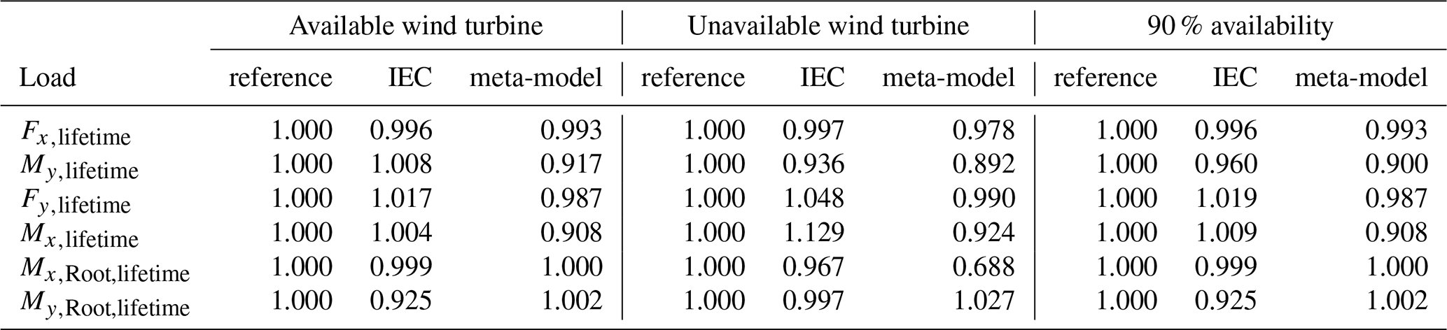
For the method according to IEC 61400-3, it becomes clear that the deviations of the lifetime DELs from the reference solution are small with less than 10 % deviation from the reference solution with the exception of M_x,lifetime for the unavailable idling case. Here, the deviation is approximately 13 %. However, assuming a typical availability of 90 % as also shown in Table 3, it is apparent that although the deviation of the lifetime DEL for M_x for the unavailable idling case is approximately 13 %, the total lifetime DEL under consideration of 90 % availability is almost unaffected by this deviation.

The lifetime DELs predicted using the meta-models also show, with two exceptions, only small deviations of less than 10 % compared to the reference solution. Only in the case of the unavailable idling wind turbine are the deviations for two internal forces (M_y,lifetime and M_{x,Root,lifetime}) larger than 10 %. One possible explanation for the poorer approximation by the meta-models is that the meta-models may not represent all the important effects that occur in the simulation model. Although the meta-models have been comprehensively validated (Müller et al., 2022; Schmidt et al., 2025a), it is possible that, due to the large number of combinations of environmental conditions considered in this study, there are input parameter combinations that the meta-models are not able to accurately represent. Therefore, possible causes will be discussed in more detail.

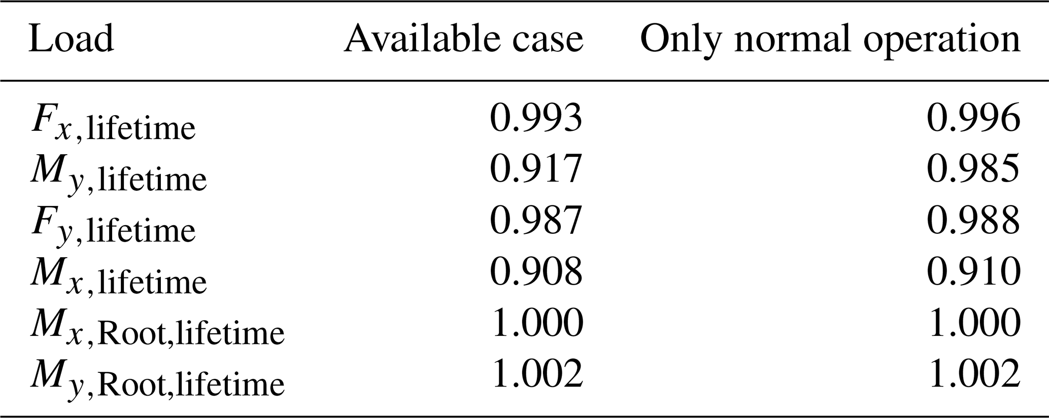
At 11 %, the deviation of M_y,lifetime for the unavailable case is of a similar magnitude to that of M_y,lifetime in the available case and also in the the 90 % availability case and M_x,lifetime for all considered cases. It therefore seems that there are overall effects on the bending moments at the monopile that cannot currently be represented by the meta-models. Since the available case includes normal operation and idling (for wind speeds outside the wind speed range for normal operation), the lifetime DELs resulting from taking only normal operation into account are now being investigated to further determine the cause of the poorer approximation quality for the bending moments at the monopile. The resulting normalised lifetime DELs are shown in Table 4. It becomes clear that the predicted lifetime DELs for the available case and for normal operation are generally very similar. Only for M_y,lifetime are the differences between the normalised lifetime DELs larger. Here, in contrast to the current study, the meta-model for M_y can predict the lifetime DELs for normal operation with a small deviation of less than 2 % compared to the reference solution. The deviation of M_y,lifetime for the available case therefore mainly arises from the prediction of the idling meta-model. During normal operation, the fore–aft direction (M_y) is significantly more damped than the side-to-side direction (M_x) of the offshore wind turbine. However, during idling, this aerodynamic damping is no longer present due to the very slow rotor speed resulting in a significant lower damping in the fore–aft direction. This different structural behaviour and the resulting larger impact of the wave loads caused by the lower damping seem to be something that the meta-models cannot handle at present. Furthermore, as described in Schmidt et al. (2025a), M_x and M_y for idling show greater seed-to-seed variation than, for example, F_x and F_y. This makes accurate predictions using meta-models even more difficult. However, a deviation of around 10 % of the lifetime DELs of the reference solution is considered acceptable within the scope of this study.

Table 4 Comparison of the normalised lifetime DELs predicted by the Kriging meta-models for the available case and for normal operation. The lifetime DELs are normalised using the reference solution for the available case and for normal operation.

For the meta-model of M_x,Root for idling conditions, it can be assumed that the important effects are not all taken into account in the meta-model. This becomes clear when looking at the predicted short-term DELs of M_x,Root as a function of individual input parameters, e.g. as a function of v_s or T_p as shown in Fig. 4. Across the entire wind speed range and also across a large range of the peak period, the meta-model underestimates the short-term DELs calculated by the simulation model. In contrast to the bending moments at the monopile, however, the deviation of M_{x,Root,lifetime} is significantly higher at approximately 31 % for the “unavailable” idling case. This is a very large deviation, which is not acceptable at first glance. Nevertheless, for the investigated offshore wind turbine, the values for M_x,Root,DEL under idling conditions are significantly smaller compared to normal operation as shown by Schmidt et al. (2025a). Therefore, for M_x,Root, idling has only a very minor impact on the overall lifetime DEL at 90 % availability of the wind turbine as shown in Table 3. As the focus of this work is not only on idling conditions, the high deviation of M_{x,Root,lifetime} for the “unavailable” case will not be addressed further in this paper. However, this is an issue that should be investigated more closely in future work, particularly if idling forms the focus of an investigation.

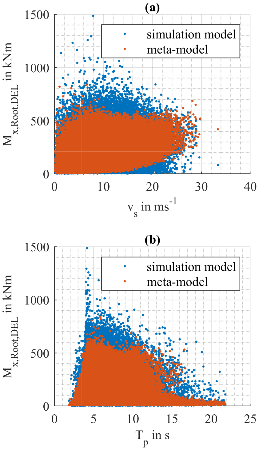
Figure 4 Comparison of the short-term DELs of M_x,Root calculated by the aeroelastic simulation and the Kriging meta-model (a) depending on v_s and (b) depending on T_p.

Another point that becomes apparent when looking at the lifetime DELs predicted with the meta-models in Table 3 is that, with a few exceptions, the predicted lifetime DELs are smaller than the lifetime DELs of the full lifetime reassessment. The calculation with the meta-models is thus not conservative. However, to safely use the meta-models as a surrogate for aeroelastic simulations for the lifetime calculations, they should be conservative compared to the original aeroelastic simulation. Therefore, this is a point that will be discussed in more detail in the further course of this study. However, even the lifetime DELs determined according to IEC 61400-3 are not conservative for all considered internal forces. As shown by Schmidt et al. (2023), these only become conservative if the 90th percentile is chosen for TI instead of the mean value as used in the current study.

3.2 Impact of the number of simulations used for the determination of the lifetime DELs

For the lifetime DELs shown in Table 3, using the method according to IEC 61400-3, 194 568 aeroelastic simulations were performed. For the meta-model-based method, 17 000 aeroelastic simulations for the training of the meta-models (8500 simulations for each of the normal operation and idling) were conducted as no more aeroelastic simulations needed to be conducted for the determination of the lifetime DELs. In this section, it is investigated to what extent these numbers of simulations can be reduced. This is an important point, as each simulation with a simulation time of 10 min also requires around 10 min of computing time.

3.2.1 Required number of simulations for lifetime reassessment using the method according to IEC 61400-3

Figure 5 shows the lifetime DELs for the case of 90 % turbine availability as a function of the simulations performed to determine the lifetime DELs, to clarify how many simulations are needed to calculated the lifetime DELs. Here, a constant number of simulations is used for the reference solution and the calculation with the meta-models. In contrast, the number of simulations for calculating the lifetime DELs according to IEC 61400-3 is increased stepwise to a maximum of 194 568 to find out how many simulations are required to achieve a good approximation to the reference solution. The stepwise increase in the number of simulations is achieved by decreasing p_min from p_min=0.1 % until $p_{\text{min}}=\mathrm{7.6}\times {\mathrm{10}}^{-\mathrm{5}}\mathit{\%}$. This is done for the input parameter combinations for the “available” case. For the “unavailable” case, for each step, the same input parameter combinations are used as for the “available” case. Subsequently, for each step, the lifetime DELs are calculated for the “available” and “unavailable” cases. As proceeded in Sect. 2.3.2, the probability of occurrence of each considered input parameter combination is corrected by the sum of all probabilities of occurrence. This ensures that the sum of all probabilities of occurrence considered in each step is equal to 1. Finally, the resulting lifetime DELs are weighted and added together according to Eq. (5). As before, the lifetime DELs for the available wind turbine are weighted with p_avail=0.9 and the lifetime DELs for the unavailable wind turbine with p_unavail=0.1.

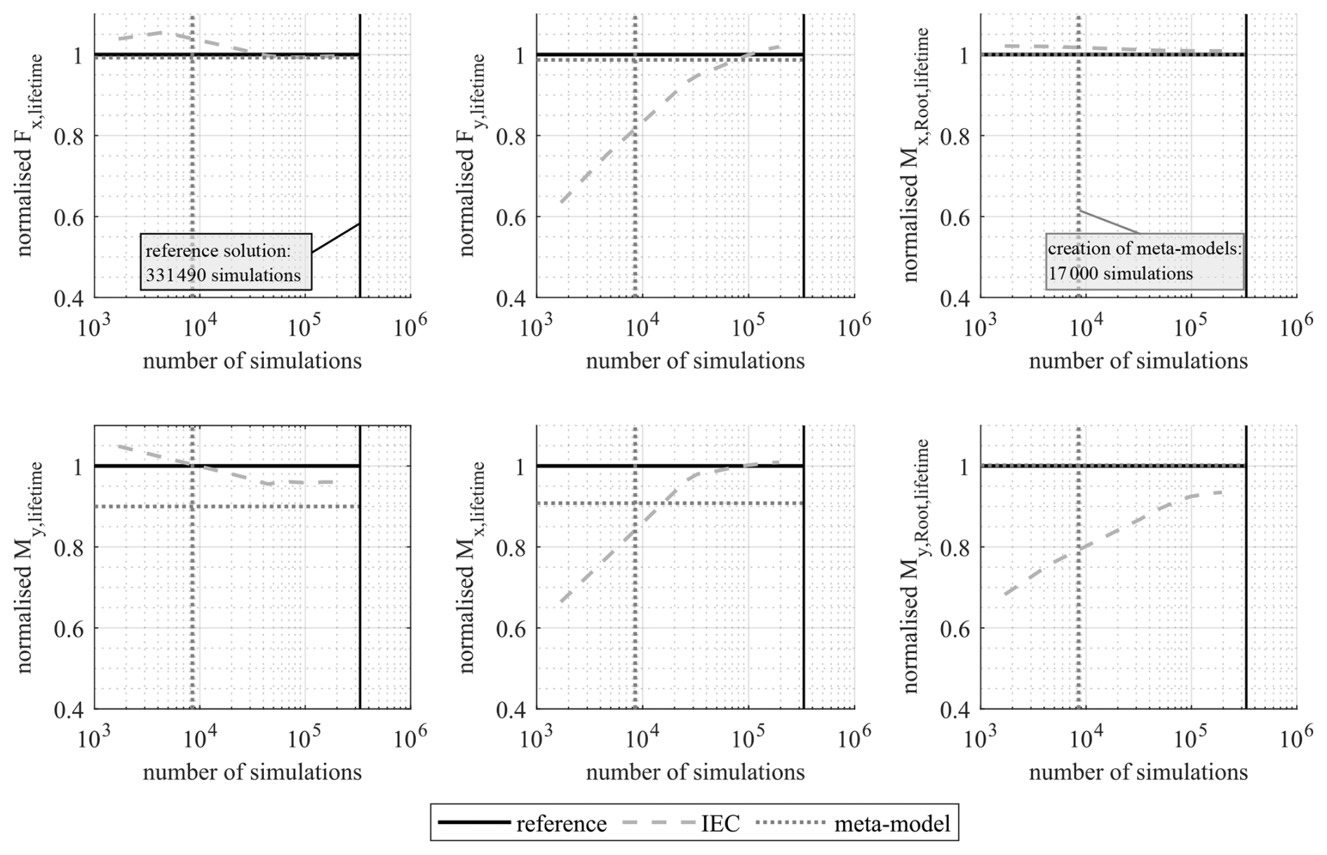
Figure 5 Normalised lifetime DELs of the three methods for the case of an availability of the wind turbine of 90 % versus the number of simulations used for the calculation of the lifetime DELs. The lifetime DELs are normalised with respect to the lifetime DELs of the reference solution.

From Fig. 5, it becomes clear that the number of simulations used for the method according to IEC 61400-3 influences the lifetime DELs of all considered internal forces. In particular, for F_y,lifetime, M_x,lifetime, and M_{y,Root,lifetime}, the number of simulations has a significant impact on the lifetime DELs. At least 70 000 simulations must be carried out to ensure that the deviation from the reference solution is less than 10 % for all considered internal forces (M_{y,Root,lifetime} is the decisive factor). Thus, the computational effort can be reduced to around 20 % compared to the reference solution. This is a significant reduction in the computational effort. However, for the prediction of the lifetime DELs using the meta-models, only 17 000 simulations were conducted for the training of the meta-models. Thus, compared to the reference solution, when using meta-models, the computing time can be reduced to around 5 % that needed for the full lifetime reassessment. Nevertheless, there might still potential for optimisation with regard to the computational effort required to determine the lifetime DELs using the Kriging meta-models. While setting up the meta-models, it was checked that the number of simulations used to train them is high enough to predict the short-term DELs with sufficient accuracy. However, for a good prediction of lifetime DELs, fewer simulations to train the meta-models are probably required, as small errors can be averaged out. It is therefore possible that the dotted vertical line in Fig. 5, which represents the number of simulations used to create the meta-models, can be shifted further to the left and the lifetime DELs will still be well predicted while additional computing time is saved. This will be investigated in more detail in the next section.

3.2.2 Required number of training samples for a lifetime reassessment using Kriging meta-models

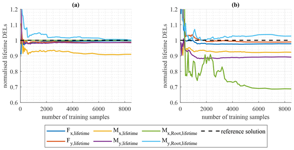
To determine the required number of training samples for a lifetime reassessment using the Kriging meta-models, convergence studies are conducted where the numbers of simulations used to create the Kriging meta-models are increased successively and the lifetime DELs are then compared with the lifetime DELs of the reference solution. Two convergence studies are carried out here: one for the meta-models representing normal operation and one for the meta-models representing idling. In the convergence study for the meta-models representing normal operation, the input parameter combinations of the available case for normal operation ($\mathrm{3}\mathrm{m}{\mathrm{s}}^{-\mathrm{1}}\le v_{\mathrm{s}}\le \mathrm{25}\mathrm{m}{\mathrm{s}}^{-\mathrm{1}}$) are used to determine the lifetime DELs. These are 190 306 input parameter combinations. The remaining 9694 input parameter combinations ($v_{\mathrm{s}}<\mathrm{3}\mathrm{m}{\mathrm{s}}^{-\mathrm{1}}$ and $v_{\mathrm{s}}>\mathrm{25}\mathrm{m}{\mathrm{s}}^{-\mathrm{1}}$) are removed, as these represent idling conditions. In the convergence study for the meta-models representing idling, the 131 490 input parameter combinations for the unavailable case can simply be used.

The results are shown in Fig. 6. It becomes clear that the lifetime DELs for normal operation converge at a significantly lower number than the 8500 training samples previously used for the generation of the meta-models. Only 600 training samples are needed for the creation of the meta-models to achieve a normalised lifetime DEL with a deviation of less than 5 %, in comparison to needing 8500 training samples. Under idling conditions, it can be seen that the lifetime DELs for the internal forces at the monopile and M_y,Root also converge very quickly. To achieve normalised lifetime DELs with a deviation of less than 5 % compared to the lifetime DELs predicted with the meta-models generated using the maximum number of 8500 training samples, only 700 training samples are required. For the meta-model for M_x,Root, it takes longer for convergence to occur. Here, only after 4400 training samples is there a deviation of less than 5 % from the lifetime DEL determined using the meta-model with the maximum number of 8500 samples. However, it has already been shown in Sect. 3.1 that if an availability of 90 % is assumed, the idling conditions of the rotor blades are of very minor importance. Therefore, if, as in this case, a typical wind turbine availability is assumed and the focus is not on idling conditions, very good predictions of the lifetime DELs can also be made for M_x,Root using the meta-model for idling trained with 700 samples. However, if the focus lies on idling conditions, the larger number of 4400 training samples should be used to create the meta-models.

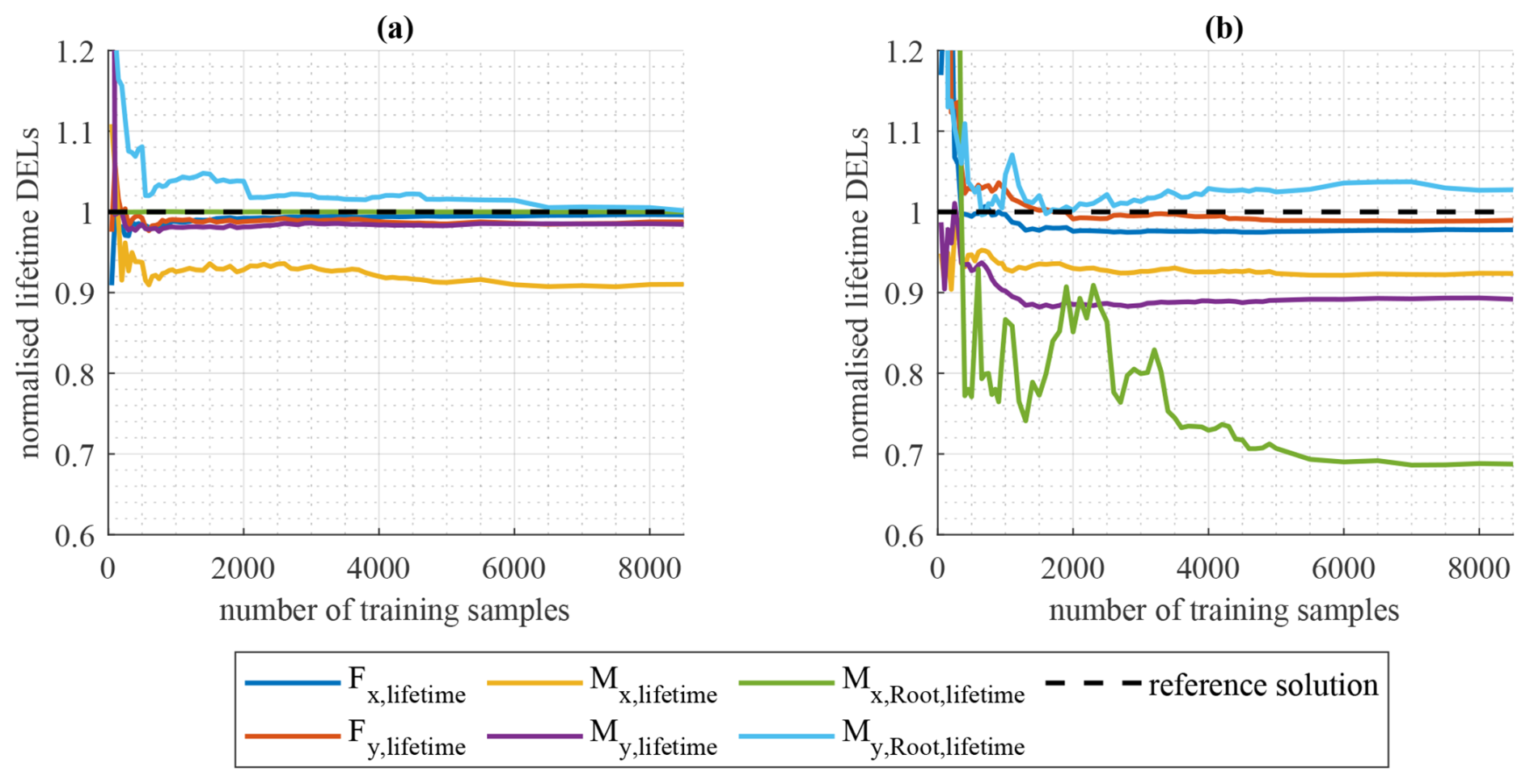
Figure 6 Predicted normalised lifetime DELs using the Kriging meta-models depending on the number of training samples used for the generation of the meta-models for (a) normal operation and (b) idling conditions. The lifetime DELs are normalised with respect to the lifetime DELs of the reference solution for normal operation and idling.

Using the recommended 600 or 700 training samples leads to errors below 5 %. However, full convergence is not yet achieved. Hence, to stay more conservative, more training samples can be used for the generation of the meta-models. For example, to achieve a maximum error of 2 % compared to the predicted lifetime DELs using the meta-models with the maximum number of training samples of 8500, 4700 samples are needed for normal operation, and, under idling conditions, 2100 samples (without considering the meta-model for M_x,Root) are needed for the generation of the meta-models. If it is desired that the prediction of M_{x,Root,lifetime} for idling also converges with an error of less than 2 %, 5500 training samples are required.

Assuming a typical availability of the wind turbine and therefore negligible impact from M_x,Root during idling, it can be summarised that the number of training samples required can be significantly reduced to a total of 1300 training samples compared to the 17 000 samples used previously. In this case, the predicted lifetime DELs for both operating states deviate by less than 5 % from the lifetime DELs predicted using the meta-models using the maximum number of training samples of 8500. This means that by using meta-models, the computing time can be reduced even further beyond the previous 5 % of the computing time of the reference solution to less than 0.5 % of the computing time of the reference solution. If higher accuracy is desired, the number of training samples can be reduced to a total of 6800, in which case the deviation from the lifetime DELs predicted using the meta-models with 8500 training samples for each operating state is only 2 %. In this case, using the meta-models reduces the computational effort to approximately 2 % of the computing time required for the reference solution.

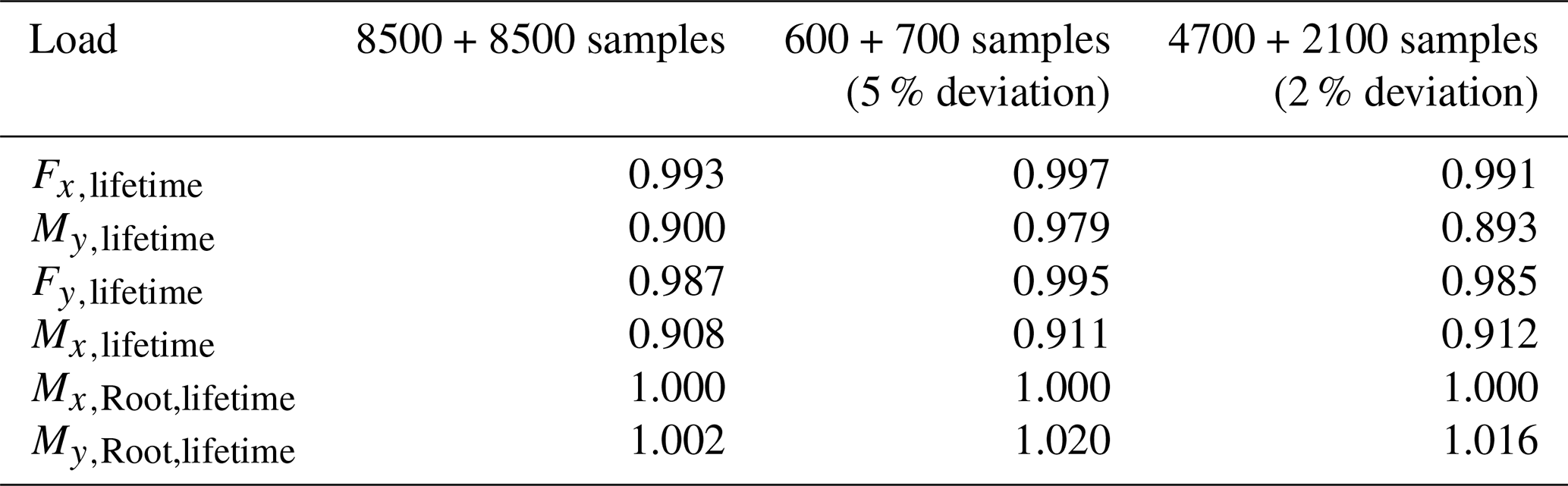
In the final step of this investigation, the lifetime DELs for 90 % availability of the wind turbine are calculated using the meta-models created using the recommended training sample sizes. These are then compared with the lifetime DELs for 90 % availability from Table 3. The results are shown in Table 5. It becomes clear that the differences arising due to the three different training sample sizes are only minor. Only M_y,lifetime predicted by the meta-models using just 1300 training samples in total deviates slightly more. This can be explained by the fact that the idling meta-model for M_y in particular has not yet converged (see Fig. 6), and the operating status idling for this internal force has a significant impact on the total lifetime DEL. However, this deviation is considered acceptable, meaning that both training set sample sizes can be recommended.

Table 5 Predicted normalised lifetime DELs using the meta-models for 90 % availability considering different training sample sizes. The first row of the table shows the training sample sizes for normal operation + training sample size for idling. The lifetime DELs are normalised with respect to the reference solution.

3.3 Conservative prediction of lifetime DELs using meta-models

As shown in Sect. 3.1, the lifetime DELs predicted by the meta-models are not yet conservative compared to the reference solution. One way to make the prediction of the meta-models more conservative is to adjust each prediction of the meta-models. As mentioned in Sect. 2.2, the Kriging meta-models used in this work generally predict a mean value and a corresponding standard deviation for each short-term DEL. The meta-models so far only use the mean value to predict the short-term DELs. Since the Kriging prediction for each short-term DEL follows a normal distribution, percentile values for each short-term DEL value can easily be calculated, e.g. the 60th percentile as shown in the following equation:

$$\begin{array}{}\text{(7)}& P_{\mathrm{60}}={\mathrm{\Phi }}^{-\mathrm{1}}\left(\mathrm{0.6}\right)\times \mathit{\sigma }+\mathit{\mu }.\end{array}$$

Here, Φ is the standard normal distribution and μ and σ are the predicted mean value and standard deviation of the Kriging meta-model. The use of another percentile for the prediction instead of the mean value has the advantage that the prediction becomes more conservative, while the already-trained meta-models can still be used. Therefore, it will be investigated to what extent a conservative prediction of the lifetime DELs can be achieved by considering a different percentile value instead of the mean value of the Kriging meta-model. While, to the author's knowledge, percentile values are not currently used to make predictions of fatigue loads using meta-models more conservative, percentile values such as the 90th percentile for TI are used in IEC 61400-1 to make predictions conservative.

For this study, the 50th percentile (mean value) to the 95th percentile are taken into account. Here, the Kriging meta-models created with 8500 training samples are used. As proceeded in the previous section (Sect. 3.2.2), two studies are conducted, one for the meta-models representing normal operation and one for the meta-models representing idling. Furthermore, the same 190 306 input parameter combinations for the determination of the lifetime DELs for normal operation and the same 131 490 input parameter combinations for the determination of the lifetime DELs for idling are used for each investigated percentile. It is assumed that the predicted lifetime DELs are conservative if the meta-models predict lifetime DELs that are greater than the lifetime DELs calculated using the reference solution. Since the lifetime DELs predicted using the meta-models are normalised using the reference solution, this means that the predicted lifetime DELs are conservative as soon as the normalised predicted lifetime DELs are larger than 1.

The results shown in Fig. 7a clearly indicate that, when using the 65th percentile of the Kriging prediction, all meta-models for normal operation make a prediction of the lifetime DELs on the safe side (normalised lifetime DEL is greater than 1). For the meta-models representing the idling wind turbine (Fig. 7b), this is only achieved from the 90th percentile upwards. Here, M_{x,Root,lifetime} is decisive. However, it is noticeable that the results of M_{x,Root,lifetime} deviate significantly from the results for the other internal forces investigated. For the remaining internal forces, the use of the 70th percentile would be sufficient to achieve a value of the normalised lifetime DELs larger than 1. One reason for the large deviation of the curve of M_{x,Root,lifetime} is that the lifetime DEL is not approximated as well by the meta-model as described before. However, as mentioned in Sect. 3.1, idling has only a very minor impact on the overall lifetime DELs of the rotor blade root bending moments, assuming a typical availability. Thus, for 90 % availability, even when using the mean value for the prediction with the meta-models, the prediction for both rotor blade root bending moments is greater than or equal to 1 (see, for example, Table 3). From this, it can be concluded that if typical availability is assumed, a non-conservative prediction of the idling meta-model of M_x,Root still leads to a conservative total lifetime DEL.

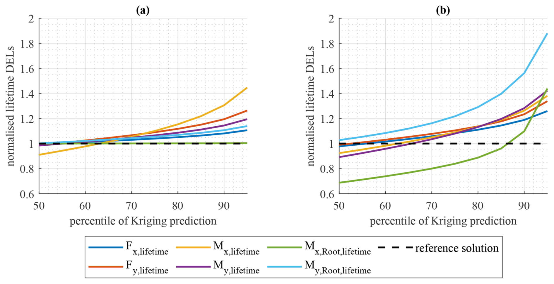
Figure 7 Normalised lifetime DELs using the Kriging meta-models depending on the percentile of prediction of the Kriging meta-models for (a) normal operation and (b) idling conditions. The lifetime DELs are normalised with respect to the lifetime DELs of the reference solution for normal operation and idling.

Assuming typical availability of the wind turbine, the use of the 65th percentile is recommended for the meta-models representing normal operation, and the use of the 70th percentile is recommended for the meta-models representing idling for the prediction of conservative lifetime DELs for all considered internal forces. However, if the focus is on idling, the 90th percentile should be used for the meta-models representing idling.

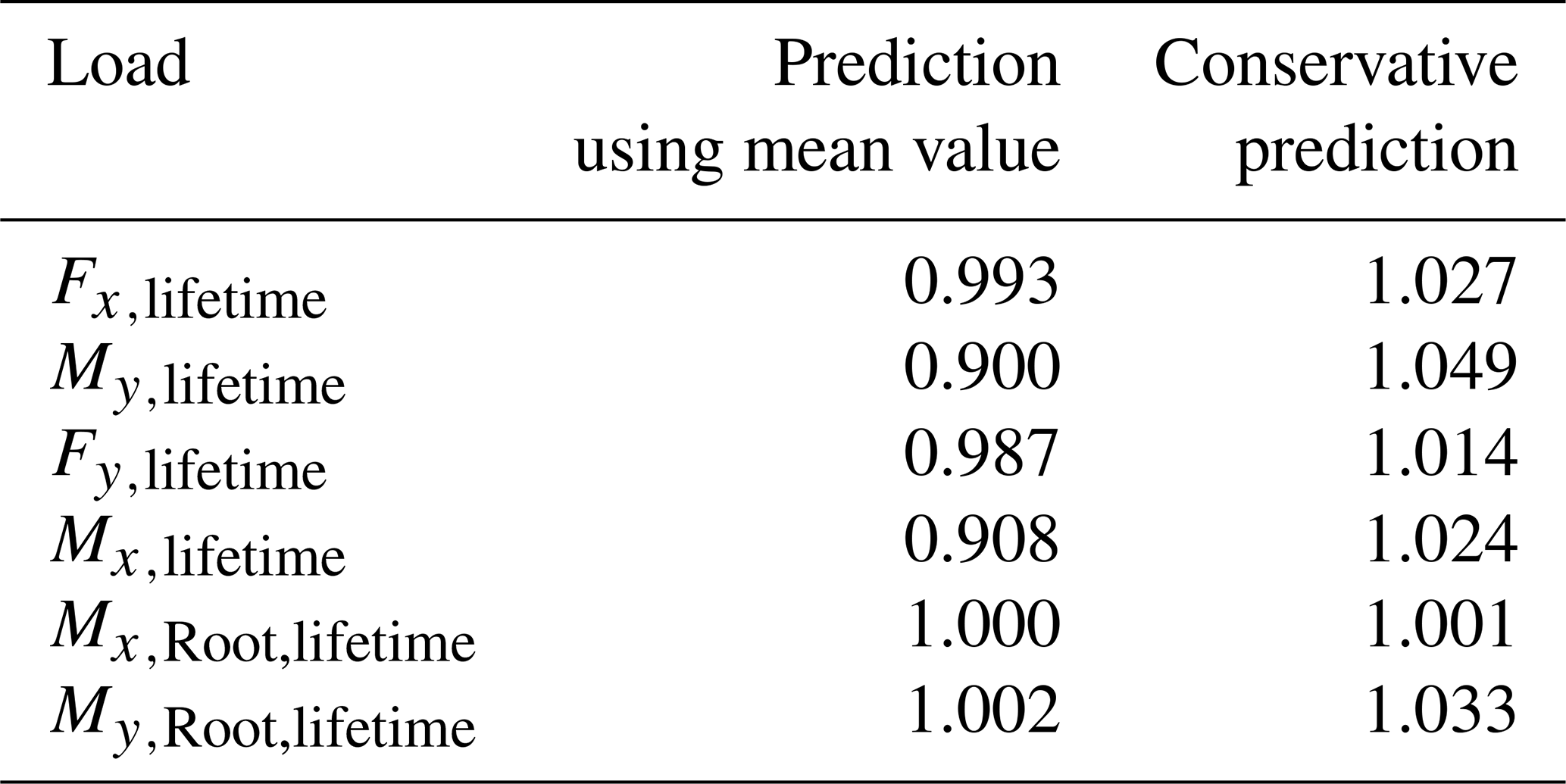
If the percentiles described above (65th percentile for normal operating and 70th percentile for idling) are used for the predictions with the meta-models, the total lifetime DELs for an availability of the wind turbine of 90 % shown in Table 6 are obtained. It becomes clear that all meta-model predictions are now conservative compared to the reference solution. Hereby, the deviation of the reference solution is below 5 % for all considered internal forces. This shows that only by using other percentiles of the Kriging predictions instead of the mean values can the prediction of conservative lifetime DELs compared to the reference solution be ensured.

Table 6 Normalised total lifetime DELs for 90 % availability using the recommended percentiles for the meta-model predictions (65th percentile for normal operation and 70th percentile for idling) compared to the normalised total lifetime DELs using the mean values for the meta-model prediction from Table 3. The lifetime DELs are normalised with respect to the reference solution.

4 Impact of wind turbine availability on lifetime DELs

In the previous sections, a wind turbine availability of 90 % was assumed. This section briefly investigates the impact to which availability influences the lifetime DELs of the considered offshore wind turbine. To this end, the availability of the wind turbine is varied between 80 % and 100 %. To determine the total lifetime DELs for the different availabilities, the lifetime DELs determined for the “available” case and the “unavailable” case are weighted according to Eq. (5) with the availabilities $p_{\text{avail}}=[\mathrm{0.8},\mathrm{0.85},\mathrm{0.9},\mathrm{0.95}]$ and $p_{\text{unavail}}=[\mathrm{0.2},\mathrm{0.15},\mathrm{0.1},\mathrm{0.05}]$. For each investigated availability, the lifetime DELs for all considered internal forces and moments are calculated using the simulated lifetime DELs of the full lifetime reassessment (reference).

The results are shown in Fig. 8. It becomes clear that for F_x,lifetime and M_y,lifetime, a reduction in availability leads to an increase in lifetime DELs. This impact is particularly strong for M_y,lifetime, so that at 80 % availability, the lifetime DEL is approximately 1.6 times greater than at 100 % availability. One possible explanation for the increase in the lifetime DELs is that the turbine is less damped in the fore–aft direction during idling due to the lack of or very slow rotation of the rotor. Thus, the wave loads have a greater impact on the structural behaviour of the turbine. For the remaining internal forces and moments, however, a reduction in availability leads to a reduction in the lifetime DELs. The side-to-side direction is, in contrast to the fore–aft direction, significantly less damped during normal operation, resulting in a minor impact of the aerodynamic damping in this direction. Accordingly, the structural behaviour in this direction does not change as significantly as in the fore–aft direction. The fact that the lifetime DELs at the monopile decrease in the side-to-side direction with decreasing availability could be explained by the fact that during idling, the loads on the turbine resulting from the rotation of the rotor are lower. For the rotor blades, the loads are also significantly lower due to the very slow rotation of the rotor compared to normal operation. Therefore, the decrease in availability leads to a decrease in the lifetime DELs and therefore to an increase in the lifetime.

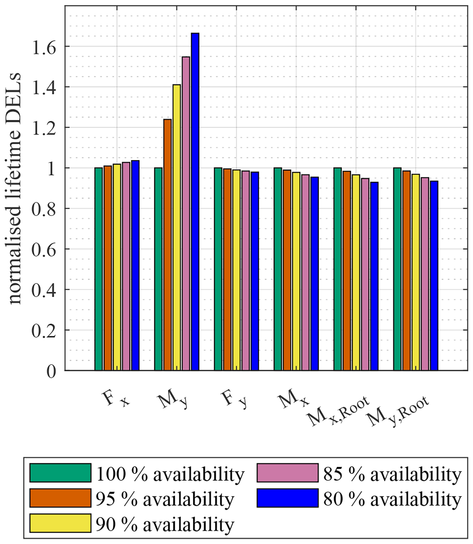
Figure 8 Normalised lifetime DELs for all considered internal forces depending on the availability of the wind turbine. The lifetime DELs are determined using the full lifetime reassessment. The lifetime DELs are normalised with respect to the lifetime DELs for the case of 100 % availability of the wind turbine.

5 Conclusions

In this study, a lifetime reassessment was performed using meta-models considering different operating conditions, namely normal operation and idling. This lifetime calculation was then compared with the results of two other methods using aeroelastic simulations: a full lifetime reassessment which served as a reference solution and a lifetime calculation according to IEC 61400-3. The simulation model used was the NREL 5 MW reference turbine on the OC3 monopile. Within the lifetime calculations, the lifetime DELs for the internal forces at the monopile at the mudline in the wind direction and perpendicular to the wind direction, as well as for the blade root moments, were determined. In summary, it can be said that both the method according to IEC 61400-3 and the meta-model-based method lead to good results regarding the lifetime reassessment. The most important findings of the investigations of the three methods for lifetime reassessment are summarised below. Furthermore, a comparison of the three methods can be found in Table 7.

1. The determined lifetime DELs using the method according to IEC 61400-3 deviate less than 15 % from the lifetime DELs of the reference solution for all three cases (“available” case, “unavailable” case, 90 % availablity). Assuming an availability of the wind turbine of 90 %, by reducing the number of simulations from 194 568 to 70 000, the computational effort for this method could be significantly reduced to around 20 % of the computational effort of the reference solution while at the same time ensuring that the deviation from the reference solution is less than 10 % for all internal forces considered.

2. For the meta-model-based method, the deviations of the lifetime DELs are, with a few exceptions, for all three cases generally small at less than 10 % compared to the lifetime DELs of the reference solution. Only for M_y,lifetime and M_{x,Root,lifetime} for the “unavailable” (idling) case are the deviations larger. While for M_y,lifetime the deviation is 11 %, the deviation for M_{x,Root,lifetime} is approximately 31 %. However, assuming a typical availability of 90 %, these deviations are not critical for the prediction of the total lifetime DELs of M_y and M_x,Root.

3. For the prediction of the lifetime DELs using the meta-models, the utilised Kriging meta-models were trained using 17 000 aeroelastic simulations (in total for both operating conditions). A convergence study showed that the number of training samples needed for the generation of the Kriging meta-models can be significantly reduced for the prediction of the lifetime DELs. Assuming a typical availability of the wind turbine, to achieve a deviation of less than 5 % compared to the lifetime DELs predicted using the meta-models with the maximum number of training samples of 8500 for each operating state, a total of only 1300 training samples are required for both operating states. This means a reduction in the computational effort to less than 0.5 % of the computational effort needed by the reference solution.

4. The predicted lifetime DELs using the meta-models are not conservative using the mean value of the prediction of the Kriging meta-models. However, using the 65th percentile for normal operation and the 70th percentile for idling leads to a conservative prediction of the lifetime DELs.

Table 7 Comparison of the three investigated methods for lifetime reassessment.

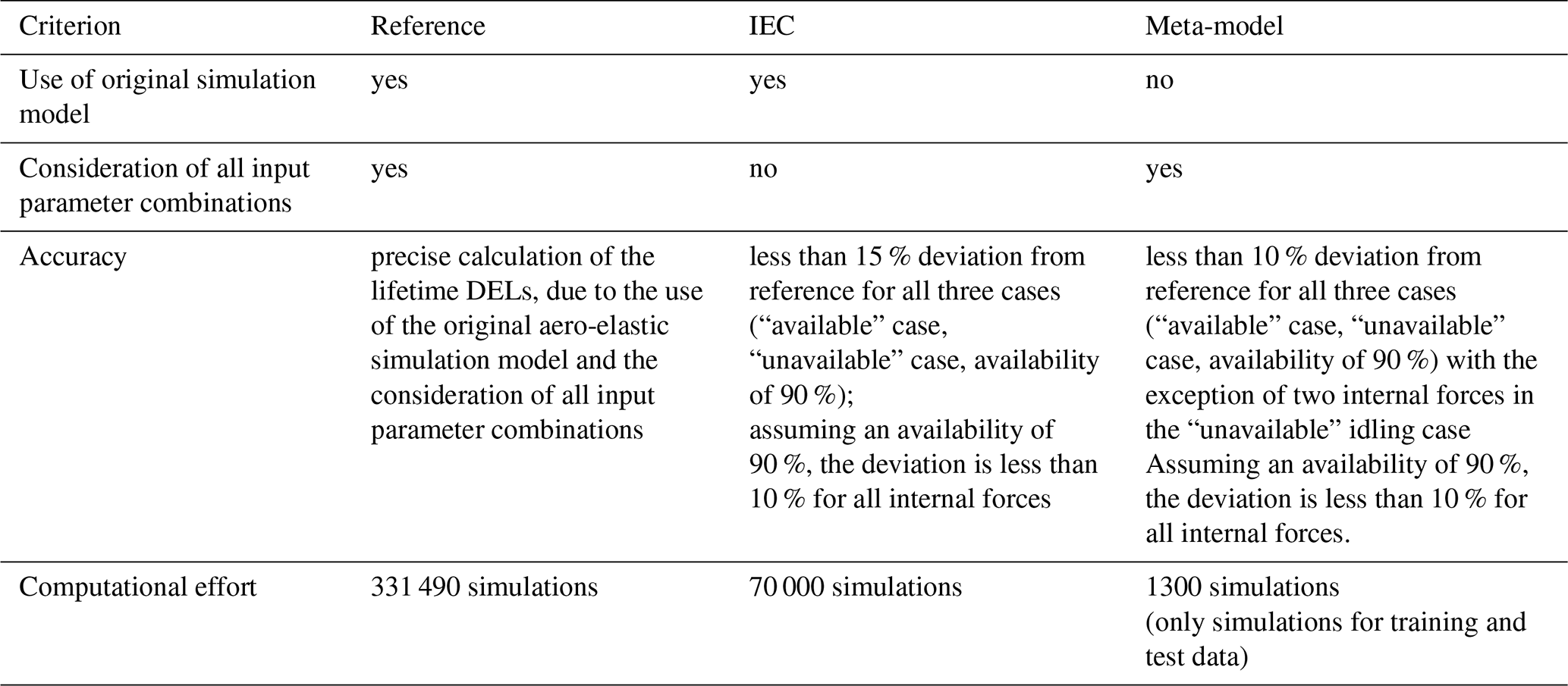
The results showed that the use of meta-models could be an alternative option to the approach according to IEC 61400-3 of reducing the number of considered input parameter combinations. By using meta-models, it is possible to consider all combinations of input parameter combinations which have actually occurred with an acceptable computational effort. The predicted lifetime DELs of the two methods are of the same order of magnitude, although the computational effort for the meta-model-based method is lower by more than an order of magnitude.

In addition to comparing the three methods for calculating the lifetime, the impact of the availability of the wind turbine on the lifetime was investigated. This investigation showed that for F_x,lifetime and M_y,lifetime (internal force and the moment at the monopile in the wind direction) a reduction in availability leads to an increase in the lifetime DELs and a resulting decrease in the remaining lifetime. For M_y,lifetime this impact is particularly strong, so that at 80 % availability, the lifetime DEL is approximately 1.6 times greater than at 100 % availability. This shows that it is very important to take idling into account when calculating the lifetime. For the remaining internal forces and moments, however, a reduction in availability leads to a reduction in the lifetime DELs.

Nevertheless, there are still a few points that remain open. The prediction of the lifetime DELs using the meta-models for the “unavailable” case for M_y,lifetime and in particular for M_{x,Root,lifetime} shows a larger deviation from the reference solution compared to the remaining internal forces considered. Here, it is assumed that these meta-models are not capable of mapping the relationship between all input parameter combinations that occur and the associated short-term DELs. This is an issue that should be investigated more closely in further research in order to improve the predictive quality of the corresponding meta-models. This is particularly important if these internal forces under idling conditions are of a similar magnitude as during normal operation, meaning that idling has a significant impact on the lifetime of the wind turbine. Furthermore, the lifetime reassessment using meta-models has only been investigated in this work for the FINO 3 site and the NREL 5 MW reference turbine on the OC3 monopile for six different internal forces at two locations of the offshore wind turbine. It is assumed that the results of this study – namely, the suitability and the required computational effort of the use of meta-models for lifetime reassessment as well as the chosen percentiles for a conservative prediction of the lifetime DELs using the meta-models – are, in principle, transferable to other sites, other types of wind turbines and/or other support structures. However, to be able to make a reliable statement on this, the transferability of the findings of this study should be investigated in more detail in future research. The findings are also expected to be transferable to onshore wind turbines. In this case, however, for a simple lifetime calculation of one onshore wind turbine, the computational effort when using meta-models may be only slightly reduced or even increased compared to the approach according to IEC 61400-1, as significantly fewer aeroelastic simulations are generally carried out for lifetime calculations of onshore wind turbines. Nevertheless, the transferability of the findings of this work to onshore wind turbines is a point that should be investigated in future work, too, since, in the case of probabilistic lifetime calculations or design optimisations (incorporating design parameters as input parameters), the computational effort increases significantly. Additionally, in this work, only Kriging meta-models were used to predict the lifetime DELs. Future work should also consider different meta-models to find out if the choice of another meta-model type will lead to a better prediction of the lifetime DELs and/or a further reduction in the required computational effort. However, Kriging has the benefit of direct uncertainty estimation, which is essential for making the meta-model conservative. It should also be noted that the use of short-term and lifetime DELs for the lifetime calculation is particularly for the rotor blades a simplification. Although this is a simplification, it is nevertheless the current state of research and also in line with industry standards with regard to lifetime reassessments and global aeroelastic simulations in the time domain.