Comment on “A theoretical upper limit for offshore wind energy extraction” by Simão Ferreira et al. (2026)

A theoretical limit for the energy extraction of offshore wind farms has been suggested by Simão Ferreira et al. (2026) based on a simple analytical model that was originally designed to provide an estimate of the turbine wake losses of an infinite wind farm. Simão Ferreira et al. (2026) validated the model with 72 offshore wind farms using an ad hoc and undocumented method to correct the model for application to finite wind farms. In this work, we discuss our concerns regarding the non-reproducibility of the finite wind farm correction and its sensitivity to the model results and validation. We conclude that the limit proposed in Simão Ferreira et al. (2026) is not a theoretical limit but rather a limit supported by model results that are strongly dependent on the non-reproducible finite wind farm correction. Therefore, the model of Simão Ferreira et al. (2026) cannot be employed to assess the feasibility of national policies.

1 Introduction

In a recent paper, Simão Ferreira et al. (2026) suggested a theoretical limit for the energy extraction of offshore wind farms in terms of the capacity factor. Simão Ferreira et al. (2026) applied simplified analytic models of a wind turbine power curve, the wind resource, and the interaction between the atmospheric boundary layer and a wind farm of infinite size. Furthermore, a largely unspecified model correction for finite wind farms is applied that depends on the wind farm layout, wind rose, and neighboring wind farms. The model is validated against measured net capacity factors of 72 offshore wind farms situated in the Baltic, North, and Irish seas. Finally, national policies for planned offshore wind farms are investigated, and some of these are stated to assume capacity factors significantly in excess of the proposed theoretical limit, especially for the Netherlands. The latter led to a public hearing in the Dutch parliament where the authors were interviewed regarding their findings. Hence, the work of Simão Ferreira et al. (2026) has had a major political impact in the Netherlands.

Simão Ferreira et al. (2026) addresses an important issue regarding the saturation of offshore wind farms in waters with limited space leading to reduced energy yield, mainly due to wind turbine and farm wake losses. The wind industry and academia have developed a range of numerical models to calculate such losses (Fitch et al. (2012), Volker et al. (2017), and Fischereit et al. (2022)), which due to their complexity and computational cost, may not be accessible to policy makers. For this reason, Simão Ferreira et al. (2026) proposed a simplified analytical model that can potentially be applied in a simple spreadsheet, based on the work of Frandsen (1992) and Sørensen and Larsen (2021).

In this paper, we address several concerns regarding the validation and application of the model in Simão Ferreira et al. (2026). We also offer a number of clarifications, as the chosen terminology in Simão Ferreira et al. (2026) can lead to misinterpretation of their results. Our main concerns are as follows.

1. The proposed limit of the capacity factor is not a theoretical limit in the same way as, for example, the Betz limit is considered to be for the power coefficient of a single turbine. Instead, the proposed limit is based on an analytical expression that is formulated using a number of heuristic model assumptions, including unknown model parameters. A different choice in these parameters can lead to distinctly different limits.

2. The plotted limit labeled as theoretical limit (solid line) in Figs. 4, 5, and 9 in Simão Ferreira et al. (2026) represents a normalized gross annual energy production (AEP), but this is not clear from the paper.

3. The validation of the analytical model with 72 wind farm in Figs. 3, 4, and 5, is not reproducible. This is because the model is corrected by manually counting the freestream turbines for each wind farm, taking into account the wind farm layout, wind rose, and neighboring wind farms. This manual approach is only briefly described by Simão Ferreira et al. (2026), while a scientific method is not provided. In addition, the model correction is very sensitive to the outcome of the validation, which is not described in Simão Ferreira et al. (2026).

4. The model validation is performed with measurements of net wind farm capacity factors. These measurements also include losses related to grid faults, curtailment, turbine availability, etc., which makes it impossible to isolate wake losses for model validation. Simão Ferreira et al. (2026) suggested an additional loss factor of 0.9 to account for this but they do not provide compelling evidence for their chosen value.

5. The analytical model of the infinite wind farm wake loss is implicit in Simão Ferreira et al. (2026) due to the need for solving a geostrophic drag law numerically. However, for the application of the 72 wind farms, the model can be expressed as a simple explicit relation that only depends on the turbine spacing, due to the use of a constant latitude, thrust coefficient, and roughness length and due to the fact that the 72 wind farms have turbines with similar hub heights in logarithmic space. It should be noted that the turbine spacing depends on the wind farm area, but the latter is mathematically undefined for a wind farm layout with a concave shape, which can lead to model uncertainties. Furthermore, the proposed wind farm wind factor mainly depends on two parameters, the finite wind farm correction and the turbine spacing, which is not clear in the work of Simão Ferreira et al. (2026).

6. Simão Ferreira et al. (2026) calculated that the Dutch national policy overestimates the analytical maximum capacity factor (assuming 10 % losses) by 49 %. However, the references provided by Simão Ferreira et al. (2026) state a range of values for the planned installed rated wind farm power per unit area, or capacity density, of between 4 and 10.5 MW km⁻², and also mention different values of the expected annual full load hours, namely 3700 and 4750–5100 h, which correspond to capacity factors in between 0.42 and 0.58. While a capacity factor of 0.58 is indeed an optimistic estimate, the lower value of 0.42 is in the range of the measured capacity factors of the 72 wind farms. In addition, given the model sensitivity to the finite wind farm correction, it is impossible to claim that the Dutch policy exceeds the modeled capacity factor by 49 %. Finally, if the planned wind farm with an installed capacity of 10 000 MW is realized, it is unrealistic to consider it as one large wind farm with a uniform turbine density. A more realistic scenario is a wind farm cluster where separate wind farms with a size of 1000–2000 MW are installed over time including space between them, which the analytical model does account for.

To understand our principal concerns with the work of Simão Ferreira et al. (2026), the main model equations are summarized and discussed in Sect. 2. The finite wind farm correction is addressed in Sect. 3, where we also compare results of an automated method with the results of the undocumented manual method of Simão Ferreira et al. (2026). Several simplifications are shown in Sect. 4, which we use to understand the main parameters of the model. Finally, we address the problems with the validation method in Sect. 5.

It should be noted that original authors have added several community comments (Sørensen et al., 2026; Simão Ferreira, 2026) during the open review process of this article. We have included their main results in the present work to show that our main concerns remain unresolved.

2 Model definition

The main model equations of Simão Ferreira et al. (2026) are repeated here. We start with a simplified model of the wind distribution at the location of a wind farm, which is the well-known Weibull distribution of wind speed, being a function of a shape parameter, k, and a scale parameter, λ:

$$\begin{array}{}\text{(1)}& f\left(U\right)={\displaystyle \frac{k}{\mathit{\lambda }}}{\left({\displaystyle \frac{U}{\mathit{\lambda }}}\right)}^{k-\mathrm{1}}\exp {\left(-{\displaystyle \frac{U}{\mathit{\lambda }}}\right)}^k,U_{\mathrm{0}}=\mathit{\lambda }\mathrm{\Gamma }\left(\mathrm{1}+\mathrm{1}/k\right).\end{array}$$

Here, U₀ is the mean wind speed and Γ is a Gamma function. Note that we use the subscript 0 to denote freestream conditions, while the subscript ∞ is used for infinite wind farm variables. Simão Ferreira et al. (2026) employed a constant Weibull shape parameter (k=2.4) for simplicity, while the Global Wind Atlas 4.0 (Davis et al., 2023) suggests that k varies between 2.0 and 2.6 for the 72 offshore wind farms.

Subsequently, a simplified model of a wind turbine power curve, P, as function of the wind speed, U, is defined as

$$\begin{array}{}\text{(2)}& \begin{array}{ll}P\left(U\right)=P_{\mathrm{r}}{\left(\frac{U}{U_{\mathrm{r}}}\right)}^{\mathrm{3}}& U\le U_{\mathrm{r}}\\ P\left(U\right)=P_{\mathrm{r}},& U_{\mathrm{r}}<U\end{array},U_{\mathrm{r}}=\mathrm{2}\sqrt[\mathrm{3}]{{\displaystyle \frac{P_{\mathrm{r}}}{\mathit{\rho }{C}_{\mathrm{P}}\mathit{\pi }{D}^{\mathrm{2}}}}}.\end{array}$$

Here, P_r is rated electric wind turbine power generation and U_r is the wind speed at which rated power is achieved. Furthermore, ρ=1.225 kg m⁻³ is the air density, C_P is the constant below-rated power coefficient, and D is the rotor diameter. The wind turbine model does not have a cut-in, U_cut-in, and cut-out wind speed, U_cut-out. For the energy yield calculations, this simplification holds if $U_{\text{cut-in}}/\mathit{\lambda }\ll U_{\mathrm{r}}/\mathit{\lambda }\ll U_{\text{cut-out}}/\mathit{\lambda }$. In Simão Ferreira et al. (2026), values of k=2.4 and C_P=0.46 are assumed for all sites.

The integration of the power curve and Weibull distribution, normalized by the rated power, leads to the capacity factor of a single turbine, which can be expressed as function of $x\equiv U_{\mathrm{r}}/\mathit{\lambda }$ and k:

$$\begin{array}{}\text{(3)}& \begin{array}{rl}{C}_{\mathrm{f},\mathrm{0}}& =f(x,k)=x^{-\mathrm{3}}\mathrm{\Gamma }\left(\mathrm{1}+{\displaystyle \frac{\mathrm{3}}{k}}\right){\mathrm{\Gamma }}_{\mathrm{ic}}\left(\mathrm{1}+{\displaystyle \frac{\mathrm{3}}{k}},x^k\right)\\ & +\exp \left(-x^k\right),\end{array}\end{array}$$

with Γ_ic as the incomplete Gamma function. The equation for C_f,0 multiplied by a loss factor for losses unrelated to wake effects, f_loss, is the analytical upper limit that Simão Ferreira et al. (2026) propose, though this is not clearly stated in their work and often misunderstood by readers of their work. Hence, the limit represents a normalized gross AEP × f_loss. The variable x is a parametric variable in Eq. (3) which gives a single line for a fixed k, which is explained in more detail in Sect. 5. This variable can also be defined as the ratio of $U_{\mathrm{r}}/U_{\mathrm{0}}$, using the constant $c_{\mathrm{0}}=\mathrm{\Gamma }\left(\mathrm{1}+\mathrm{1}/k\right)$ from Eq. (1). Furthermore, Eq. (3) is reused several times by Simão Ferreira et al. (2026) (their Eqs. 12, 13, and 16), but it is the same as Eq. (3) with different x definitions.

For an infinite wind farm with uniform turbine spacing, the model of Frandsen (1992) and Sørensen and Larsen (2021) can be used to calculate the corresponding wake loss:

$$\begin{array}{}\text{(4)}& \begin{array}{rl}& {\mathit{\epsilon }}_{\mathrm{\infty }}={\displaystyle \frac{U_{\mathrm{\infty }}}{U_{\mathrm{0}}}}={\displaystyle \frac{\mathrm{1}+\frac{\mathit{\gamma }}{\mathit{\delta }}}{\mathrm{1}+\frac{\mathit{\gamma }}{\mathit{\kappa }}\sqrt{\frac{\mathit{\pi }{C}_{\mathrm{T}}}{\mathrm{8}{s}^{\mathrm{2}}}+{\left(\frac{\mathit{\kappa }}{\mathit{\delta }}\right)}^{\mathrm{2}}}}},\mathit{\gamma }=\ln \left({\displaystyle \frac{G}{f^{\prime }h}}\right),\\ & \mathit{\delta }=\ln \left({\displaystyle \frac{h}{z_{\mathrm{0}}}}\right),s={\displaystyle \frac{\sqrt{A_{\mathrm{wf}}}}{D\left(\sqrt{N_{\text{tot}}}-\mathrm{1}\right)}},f^{\prime }=f\cdot e^{\mathrm{4}},\end{array}\end{array}$$

with κ=0.4 as the von Kármán constant, G as the geostrophic wind speed, f as the Coriolis parameter based on the wind farm latitude, h as the turbine hub height, $z_{\mathrm{0}}={\mathrm{10}}^{-\mathrm{4}}$ m as the offshore roughness length, C_T=0.75 as a constant turbine thrust coefficient, and s as the turbine spacing normalized by the rotor diameter, which depends on the wind farm area, A_wf, and the total number of turbines in the wind farm, N_tot. It should be noted that the use of constant thrust and power coefficients are not realistic assumptions. For large wind farms, $\sqrt{N_{\text{tot}}}\gg \mathrm{1}$, one can express the normalized turbine spacing in terms of installed wind farm power, P_wf, per unit area: $s\approx \sqrt{\mathit{\rho }{C}_{\mathrm{P}}\mathit{\pi }{U}_{\mathrm{r}}^{\mathrm{3}}/\mathrm{8}}/\sqrt{P_{\mathrm{wf}}/A_{\mathrm{wf}}}$. Equation (4) can be used to calculate the geostrophic wind speed using an iterative numerical method by setting C_T=0. Furthermore, Eq. (4) can be used to calculate the capacity factor of an infinite wind farm C_f,∞ by the substitution of $x=c_{\mathrm{0}}{U}_{\mathrm{r}}/\left(\mathit{\lambda }{\mathit{\epsilon }}_{\mathrm{\infty }}\right)$ in Eq. (3). The latter is an analytical model for the lower limit of the wind farm capacity factor. It should be noted that the infinite wind farm wake loss may never be reached for a large finite wind farm. For example, Volker et al. (2017) showed that a wind farm covering an area of 10⁵ km² has not yet reached a wake loss limit. The latter was obtained from mesoscale simulations including a simplified wind farm model representing a square wind farm using a wind farm length of 338 km, and a range of uniform turbine spacing and wind climates. Furthermore, alternative infinite wind farm models exist, as, for example, the model of Calaf et al. (2010), who suggested modification of the model of Frandsen (1992), based on large-eddy simulations of infinite wind farms using finite wind farms with lateral periodic boundary conditions. These infinite wind farm models rely on a geostrophic draw law that is commonly expressed by two constants (A and B), which can be shown to depend on atmospheric conditions, as atmospheric stability (Floors et al., 2023), boundary layer height (van der Laan et al., 2020), and capping inversion (Liu et al., 2021).

Simão Ferreira et al. (2026) introduced the wind farm wind factor, $\mathit{\varphi }=U_{\mathrm{r}}/\left(U_{\mathrm{0}}\mathit{\epsilon }\right)$, which represents $x=c_{\mathrm{0}}/\mathit{\lambda }\mathit{\varphi }$ in Eq. (3). The wind farm wind factor corrects the mean wind speed or Weibull-scale parameter to account for wake losses. It is well known that wake losses are strongly dependent on atmospheric conditions, such as ambient turbulence intensity and atmospheric stability (Porté-Agel et al., 2020). Therefore, one can argue that the collapse of the wake losses into a single variable, ϕ, may not be possible. It should be noted that ε in ϕ is the wake loss for a finite wind farm. An additional model is required to calculate the capacity factor of a finite wind farm, C_f, from C_f,0 and C_f,∞, and this is discussed in detail in Sect. 3. Furthermore, Simão Ferreira et al. (2026) also included external wind farm wake losses in their finite correction model. Simão Ferreira et al. (2026) set C_f equal to Eq. (3) and solved for x using a numerical root finding method, from which ϕ can be calculated. An important realization is that for ε=1, we obtain the normalized gross wind farm AEP limit that is referred to as the theoretical limit in Simão Ferreira et al. (2026), which is often misunderstood by readers of this work.

Although not mentioned by Simão Ferreira et al. (2026), cut-in and cut-out wind speeds of 3 and 25 m s⁻¹ are employed when calculating the wind farm capacity factor (shown in Fig. 3 and listed in Table S1 by Simão Ferreira et al., 2026) using a wind turbine power curve model with cut-in and cut-out wind speeds, as used by Sørensen and Larsen (2021). Furthermore, a model of the thrust coefficient above rated wind speed is employed using a decay exponent 3.2, as discussed in van der Laan et al. (2022). However, the cut-in and cut-out wind speeds and associated models of the power curve and thrust coefficient are not used when calculating the wind farm wind factor ϕ.

3 Model correction for finite wind farms

The model summarized in Sect. 2 can provide two values of the capacity factor, representing a normalized gross AEP, C_f,0, and a capacity factor including wake losses for an infinite wind farm, C_f,∞. These values provide analytical bounds of the capacity factor of a finite wind farm. Sørensen and Larsen (2021) introduced a model to interpolate between C_f,0 and C_f,∞ to obtain a capacity factor of a finite wind farm, C_f:

$$\begin{array}{}\text{(5)}& C_{\mathrm{f}}=w{C}_{\mathrm{f},\mathrm{0}}+\left(\mathrm{1}-w\right)C_{\mathrm{f},\mathrm{\infty }},w={\displaystyle \frac{N_{\text{free}}}{N_{\text{tot}}}},\end{array}$$

with w as a weight determined from the ratio of freestream turbines, N_free, to the total number of turbines. The problem with this method is that the weight has a large impact on C_f and it is not trivial to obtain the weight for real finite wind farms that range in size and can have irregular shapes, as well as non-uniform turbine spacing. Sørensen and Larsen (2021) determined N_free by assuming a square regular turbine layout, $N_{\text{free}}=a\sqrt{N_{\text{tot}}}$, and initially proposed a=3, later revised to a value between 4.1 and 5.9 (Sørensen et al., 2024) based on a fit using an engineering wake model applied to six offshore wind farms. This gave a corresponding average value of a=5.3. One problem with this method is that the weighting variable can become larger than one for a wind farm with fewer turbines than a² (i.e., fewer than 29 for a=5.3). Hence, one should limit the weight to one. In a non-peer-reviewed work, Simão Ferreira (2024) proposed an alternative approach by determining the weight as

$$\begin{array}{}\text{(6)}& N_{\text{free}}=M_{\text{rows}}{M}_{\text{turbines}},\end{array}$$

where M_rows=2.5 and M_turbines is the number of wind farm edge turbines that operate in freestream conditions. It is not clear why the value of M_rows is set to 2.5. Simão Ferreira et al. (2026) determined M_turbines manually for a given wind farm layout, wind rose, and neighboring wind farms, and their results were provided in a database (Simão Ferreira, 2024). However, a scientific method was not provided, meaning that one cannot reproduce the results given in Simão Ferreira (2024). In this work, we have made an attempt to automate the manual method by calculating M_turbines as follows, performed for each wind farm layout as follows.

1. A concave polygon shape is fitted to determine the edge turbine and the connections between them.

2. An outward normal vector for each edge turbine is calculated by taking the average of the outward normal vectors of the neighboring connecting edge lines.

3. For each wind direction sector, l, with steps of 30°, the dot product of the wind direction vector (representing the sector midway direction, ${\stackrel{\mathrm{‾}}{\mathit{\theta }}}_l$), with the turbine outward normal vectors, ${\stackrel{\mathrm{‾}}{n}}_{\mathrm{t}}$, is calculated, and the inflow edge turbines, M_turbines,l, are flagged for ${\stackrel{\mathrm{‾}}{\mathit{\theta }}}_l\cdot {\stackrel{\mathrm{‾}}{n}}_{\mathrm{t}}<\mathrm{0}$.

4. The inflow edge turbines are removed if they are in the shadow of an upstream wind farm located within a distance L using a ray casting method.

5. The number of remaining inflow edge turbines for all sectors is aggregated using a wind rose frequency, f_l; $M_{\text{turbines}}={\mathrm{\Sigma }}_{l=\mathrm{1}}^{l=\mathrm{12}}{f}_l{M}_{\mathrm{turbines},l}$.

The wind rose is taken from the Global Wind Atlas 4.0 (Davis et al., 2023). The wind farm layouts are obtained from the Open European offshore wind turbine database (Fischereit et al., 2025) with the exception of the Fryslân offshore wind farm layout, which is taken from the Open Street Map database (OpenStreetMap contributors, 2026).

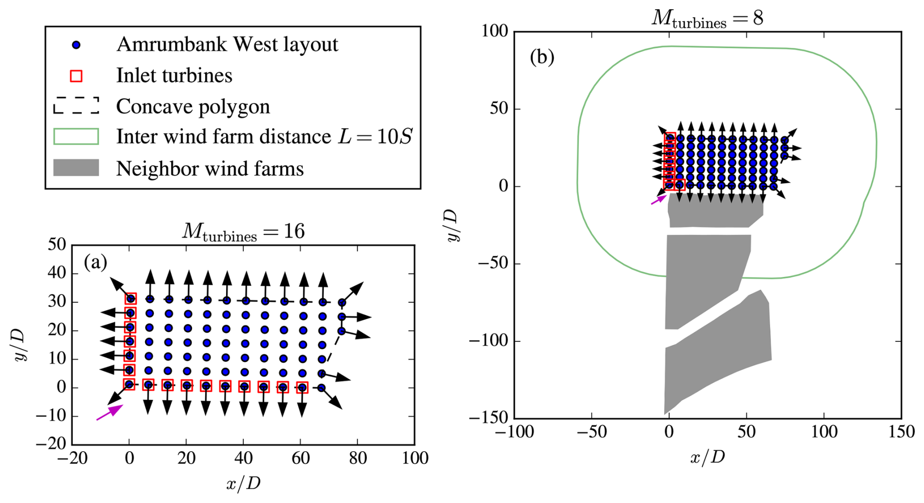
Figure 1 Example of the automated method for determining the number of freestream edge turbines, M_turbines, of the Amrumbank West offshore wind farm. (a) Without considering neighboring wind farms, (b) considering neighboring wind farms. The black arrows are the turbine outwards normal vectors and the magenta arrow is the wind direction set to 240°.

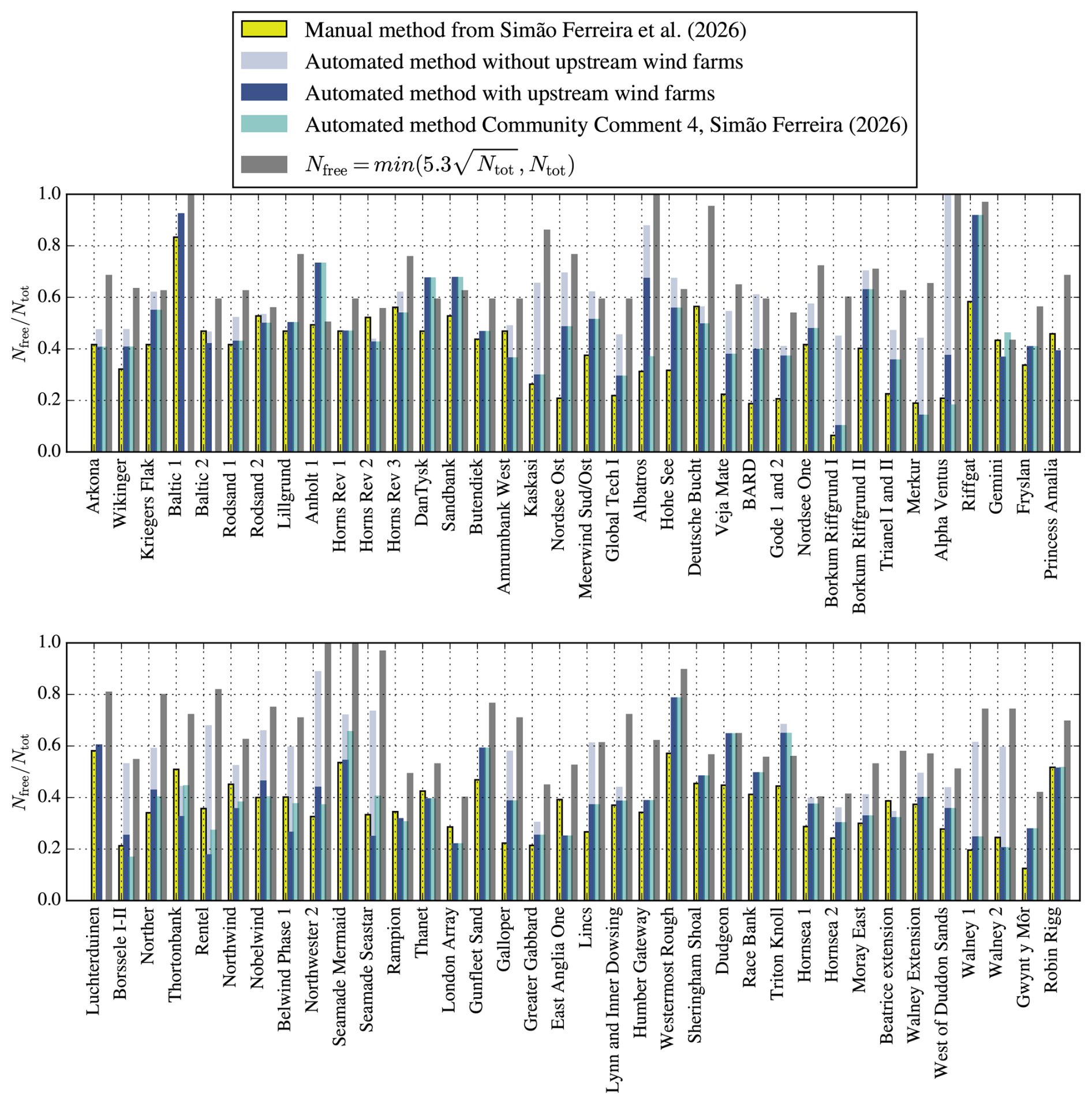
Figure 2 Results of automated model correction for finite wind farms compared to Simão Ferreira et al. (2026). Community Comment 4 (Simão Ferreira, 2026) did not calculate results of Baltic 1, Baltic 2, Princess Amalia, and Luchterduinen.

An example of our automatic method is shown in Fig. 1, where the Amrumbank West offshore wind farm layout is used. Figure 1a depicts a concave polygon (although it has become convex for the present example), the edge turbines, and the obtained freestream turbines for a wind direction of 240°, namely, M_turbines=16. It is clear that the polygon does not find all edge turbines at the eastern side of the farm, and this is related to the fact that a concave polygon requires an additional parameter that determines how tightly the polygon follows the wind farm layout shape, meaning that the number of edge turbines is not unique and user dependent. The Amrumbank West wind farm is part of the N4 wind farm cluster, and the upstream neighboring wind farms are used to filter the freestream turbines if they are located in their wake with a distance $L=\mathrm{10}S=\mathrm{59}D$, which reduces M_turbines to 8. These steps are then repeated for all 12 sectors and the results are averaged using weights from the wind rose frequency leading to M_turbines=11.3. The manual method of Simão Ferreira et al. (2026) reported M_turbines=15 in Simão Ferreira (2024) for this wind farm.

The results of our automated method are compared with the results of the manual method of Simão Ferreira et al. (2026) in terms of the ratio of freestream turbines to the total number of turbines in Fig. 2. Our results are shown including and excluding upstream wind farms (Step 4). Our automated method has been further developed by the original authors, published as Community Comments 4 (Simão Ferreira, 2026), and the results are shown in Fig. 2. The further developments include a reduction in M_rows for wind farms smaller than 25 wind turbines, special treatment of several wind farms that have inter-twined layouts or large gaps, and the use of 36 wind direction sectors. In addition, the results of the analytical method of Sørensen et al. (2024) with a=5.3 are also shown in Fig. 2. Sørensen et al. (2024) never intended to use their method for including effects of the wind rose and neighboring wind farms; therefore, the comparison of their model results shown in Fig. 2 should not be compared directly with the other results. Overall, our method replicates the trends of Simão Ferreira et al. (2026) when taking upstream wind farms into account. However, there are also large differences, for example, for the Anholt offshore wind farm, possibly because many turbines are located at the edge of the farm. The results of Community Comment 4 (Simão Ferreira, 2026) show that the original authors are not able to reproduce the results of their own ad hoc finite correction factor; large differences (above 30 %) are obtained for 20 wind farms: Anholt, DanTysk, Nordsee Ost, Hohe See, Veja Mate, Bard, Gode 1 and 2, Borkum Riffgrund I, Borkum Riffgrund II, Trianel I and II, Merkur, Riffgat, Rentel, London Array, Galloper, East Anglia One, Dudgeon, and Triton Knoll. This shows that the ad hoc method of finite correction factor of Simão Ferreira et al. (2026) remains non-reproducible. The impact of the different methods of obtaining N_free is large and is described in Sect. 5

It should be noted that we do not recommend our automated method to be used as a correction for finite wind farms situated in a wind farm cluster. For example, it is not trivial to determine the distance, L, at which upstream wind farm wakes should be taken into account. In addition, the original model from Frandsen (1992) and Sørensen and Larsen (2021) was developed for uniformly spaced wind farms excluding effects of the wind rose, wind farm layout, and upstream wind farms. In our opinion, a better application of the model is to include a wind farm cluster as one large wind farm with an effective turbine spacing, although the results may not compare well with higher fidelity models.

4 Model simplifications and main parameters

The model from Simão Ferreira et al. (2026) is implicit, but it can be shown that a simple explicit expression for ε_∞ and ϕ can be derived when the model is applied to the 72 wind farms. These simplifications are not used in the model validation of Sect. 5. However, it allows us to better understand the main model parameters.

The equation for the infinite wind farm wake loss (Eq. 4) is implicit due to the need for solving the geostrophic drag law (Eq. 4 using C_T=0). However, for the 72 offshore wind farms investigated by Simão Ferreira et al. (2026), ε_∞ can be approximated with a simple explicit expression, which was not shown in their work:

$$\begin{array}{}\text{(7)}& \begin{array}{rl}& {\mathit{\epsilon }}_{\mathrm{\infty }}={\displaystyle \frac{\mathrm{1}+c_{\mathrm{1}}}{\mathrm{1}+\sqrt{\frac{c_{\mathrm{2}}}{s^{\mathrm{2}}}+c_{\mathrm{1}}^{\mathrm{2}}}}},c_{\mathrm{1}}={\displaystyle \frac{\mathit{\gamma }}{\mathit{\delta }}}\approx \mathrm{0.219},\\ & c_{\mathrm{2}}={\displaystyle \frac{\mathit{\pi }{C}_{\mathrm{T}}{\mathit{\gamma }}^{\mathrm{2}}}{\mathrm{8}{\mathit{\kappa }}^{\mathrm{2}}}}\approx \mathrm{16.5}.\end{array}\end{array}$$

Here, the only remaining variable is the normalized turbine spacing, s. The simple expression approximates Eq. (4) to within 2.3 % for all 72 wind farms, and a comparison with the model results are shown in Fig. 3. The reason why this simplification can be made is because Simão Ferreira et al. (2026) used constant values for the roughness length and thrust coefficient. Furthermore, the latitudes of the all investigated wind farms are similar (between 50.7 and 58.5°) leading to Coriolis parameters in the range between $\mathrm{1.12}\times {\mathrm{10}}^{-\mathrm{4}}$ and $\mathrm{1.24}\times {\mathrm{10}}^{-\mathrm{4}}$ s⁻¹. In addition, the ratio of hub height to roughness length, $h/z_{\mathrm{0}}$, and the ratio of the geostrophic wind speed to hub height, $G/h$, are very similar in logarithmic space for the 72 wind farms, leading to values in the range between $\mathrm{13.3}<\mathit{\delta }<\mathrm{14.0}$ and $\mathrm{2.71}<\mathit{\gamma }<\mathrm{3.36}$, with corresponding mean values δ=13.7 and γ=3.01, respectively. The mean values of δ and γ, together with the parameters that are chosen as constants by Simão Ferreira et al. (2026), are used to obtain c₁ and c₂. It should be noted that for much taller turbines, i.e., h≫100 m, the approximation may not hold.

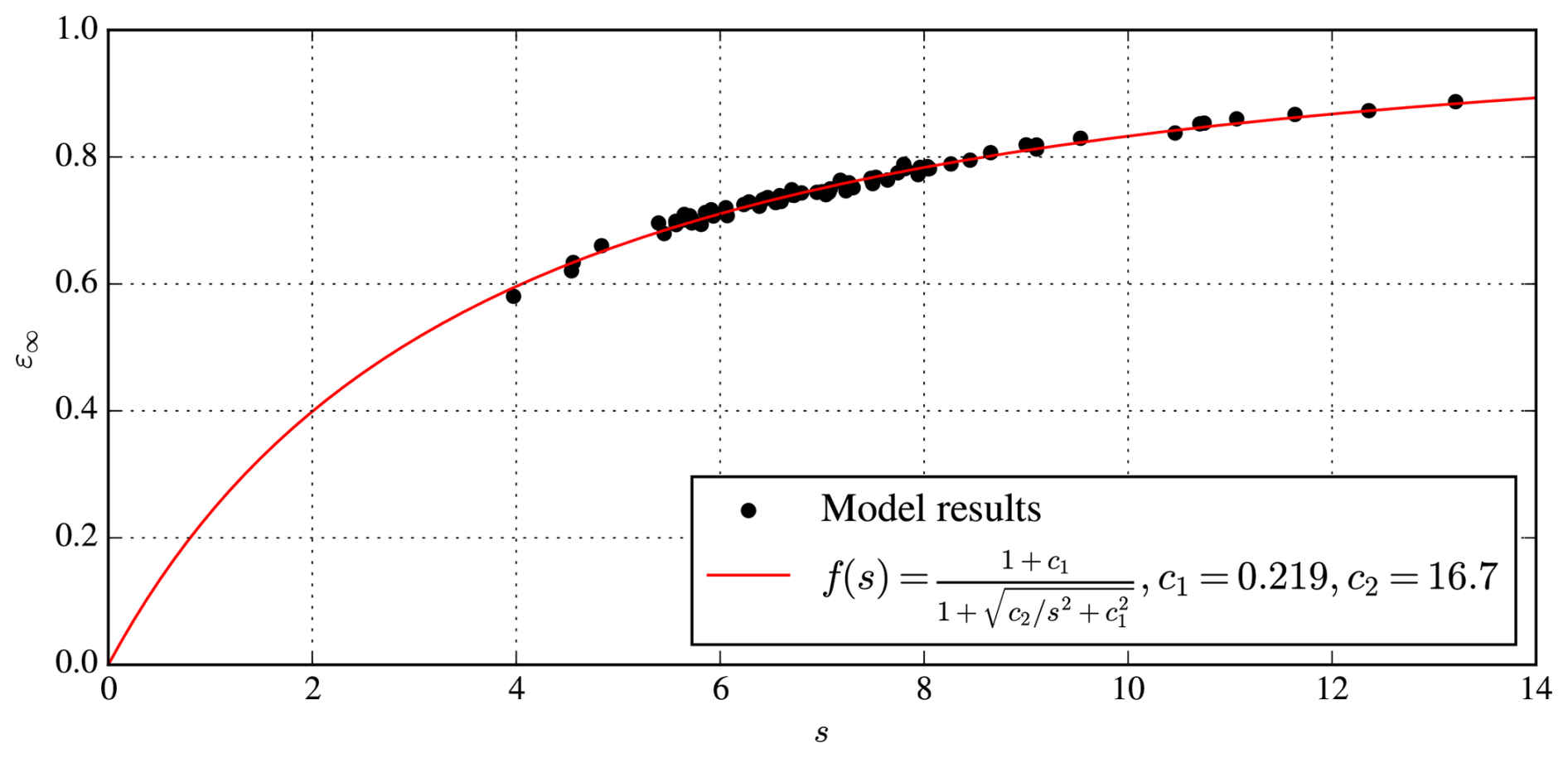
Figure 3 Comparison of model results of Simão Ferreira et al. (2026) and simplified expression (Eq. 7) for the infinite wind farm wake loss, ε_∞.

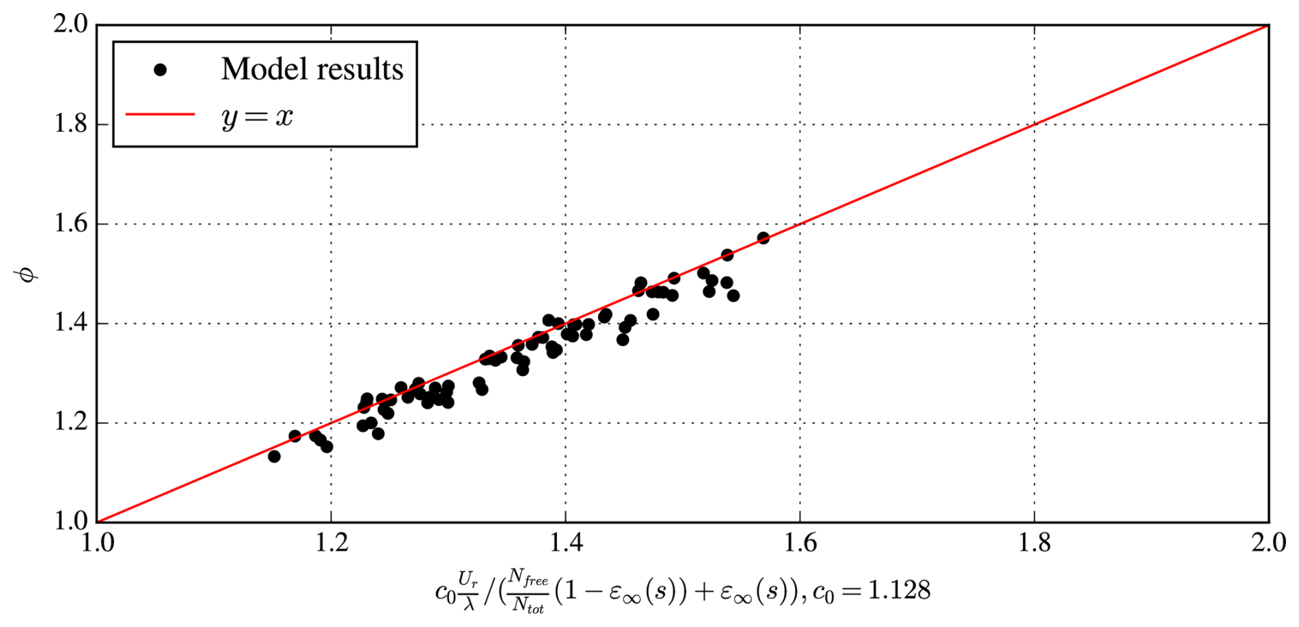
Figure 4 Comparison of model results of Simão Ferreira et al. (2026) and simplified expression (Eq. 8) of the wind farm wind factor, ϕ.

The wind farm wind factor, ϕ, is solved numerically by Simão Ferreira et al. (2026), by setting C_f equal to Eq. (3). However, one can show that for the present database of 72 offshore wind farms, ϕ can be approximated with the following explicit relationship using ε_∞ from Eq. (7):

$$\begin{array}{}\text{(8)}& \mathit{\varphi }\approx c_{\mathrm{0}}{\displaystyle \frac{U_{\mathrm{r}}}{\mathit{\lambda }}}{\displaystyle \frac{\mathrm{1}}{\frac{N_{\mathrm{free}}}{N_{\mathrm{tot}}}\left(\mathrm{1}-{\mathit{\epsilon }}_{\mathrm{\infty }}\left(s\right))+{\mathit{\epsilon }}_{\mathrm{\infty }}(s)\right)}}.\end{array}$$

A comparison of ϕ using the implicit method of Simão Ferreira et al. (2026) and our explicit expression of Eq. (8) is shown in Fig. 4. The maximum difference with the implicit calculation method of Simão Ferreira et al. (2026) is 6 %. This shows that the main parameters to calculate ϕ are the finite wind farm correction factor $N_{\text{free}}/N_{\text{tot}}$ and the normalized turbine spacing s, which is further motivated from the fact that $U_{\mathrm{r}}/\mathit{\lambda }$ is often of the order of 1.

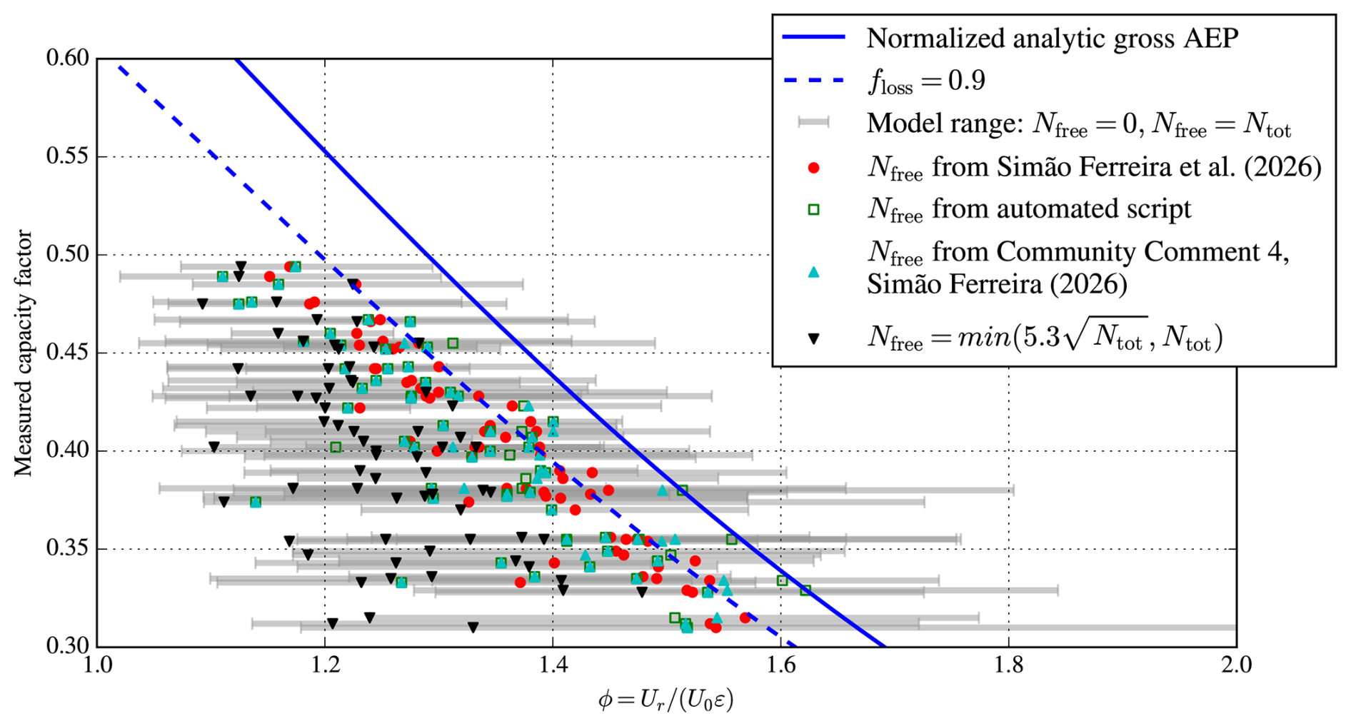
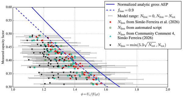
Figure 5 Measured capacity factor as function of modeled wind farm wind factor, ϕ, using different models of the finite wind farm corrections.

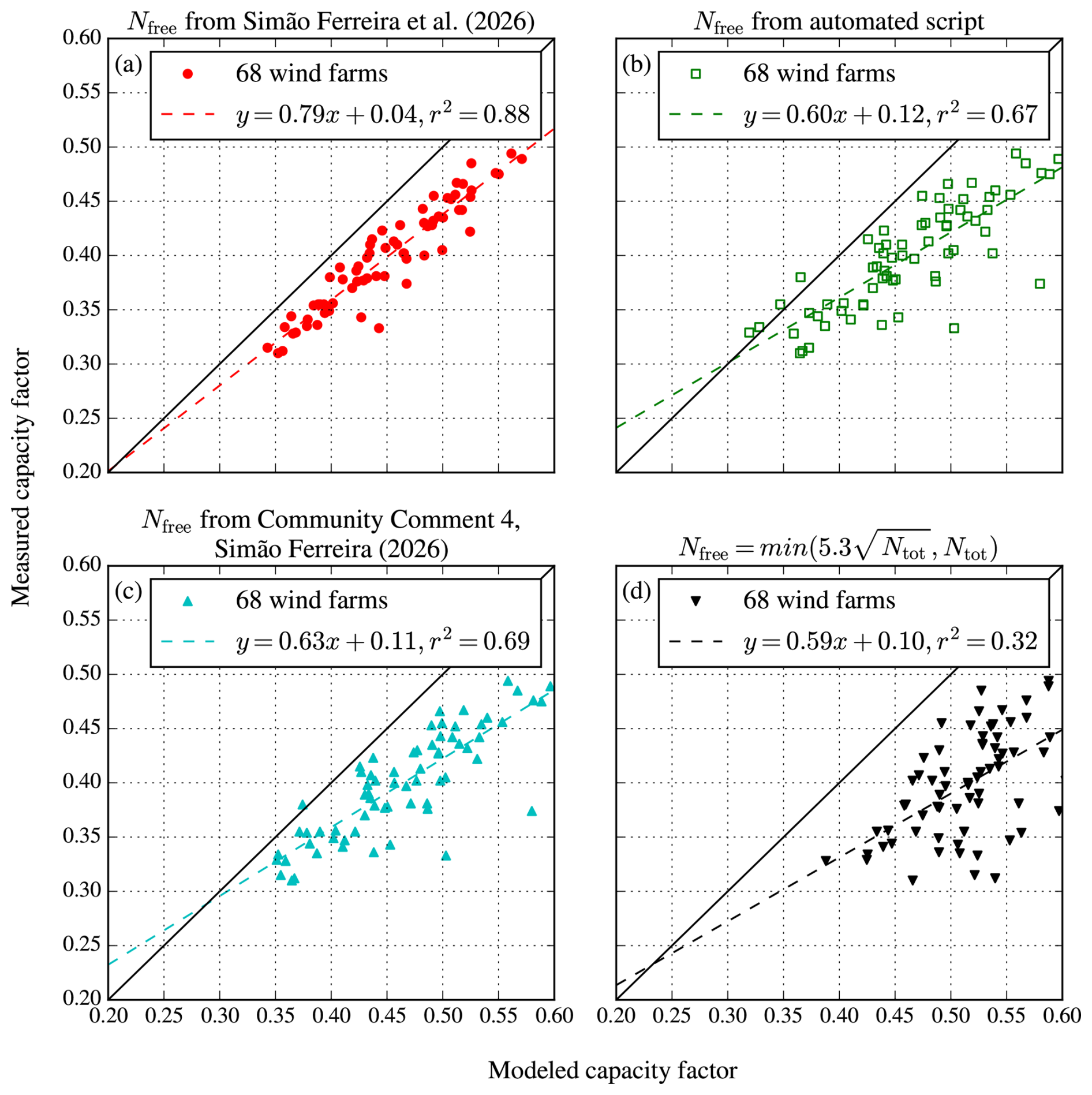
Figure 6 Measured vs. modeled capacity factor as using different models for N_free compared to Simão Ferreira et al. (2026).

5 Model validation

Simão Ferreira et al. (2026) validated their model with measured capacity factors from 72 offshore wind farms. It is important to note that these measured capacity factors include losses from wake effects and any other losses, such as grid losses, curtailment, and turbine availability. The main validation was performed by plotting the net measured capacity factor as a function of the wind farm wind factor $\mathit{\varphi }=U_{\mathrm{r}}/\left(U_{\mathrm{0}}\mathit{\epsilon }\right)$, where U_r is the rated wind speed (Eq. 2), U₀ is the mean wind speed (Eq. 1), and ε is the modeled wake loss for a finite wind farm. Figure 5 depicts four results for ϕ, where the model implementation of Sørensen et al. (2024) (MinimalisticPredictionModel) in PyWake v2.6.18 (Pedersen et al., 2023) is employed, and with different models of the finite wind farm correction in terms of N_free. The first model results in Fig. 5 (red dots) employ the ad hoc finite correction factor of Simão Ferreira et al. (2026) and replicate their original results (Table S1 of Simão Ferreira et al. (2026)), as shown in Appendix A. We disregard the results of four wind farms, Baltic 1, Baltic 2, Princess Amalia, and Luchterduinen, because their measured capacity factors were only available in pairs (Baltic 1 – Baltic 2 and Princess Amalia – Luchterduinen), not individually. Figure 5 also includes the normalized analytical model gross AEP (Eq. 3 using x as a parametric variable) and the corresponding analytical model result × a loss factor of 0.9. The model only determines the location of x in Fig. 5. However, since the model is heavily dependent on the model correction for finite wind farms, $N_{\text{free}}/N_{\text{tot}}$, this x location can vary between ε=1 (no wake losses, N_free=N_tot) and ε=ε_∞ (infinite wind farm wake losses, N_free=0). The latter is depicted as a model range in Fig. 5, which shows that the model of the finite wind farm correction has a large influence on ϕ. The left and right error bar symbols reflect no wake losses and infinite wind farm wake losses. This means that a data point moves to the right and can even cross the normalized analytic gross AEP for N_free→0. The fact that a data point can cross the normalized gross AEP is a serious issue with the validation presented by Simão Ferreira et al. (2026). If one would make sure to calibrate the model to get the correct asymptotic behavior where a data point would lie on top of the normalized gross AEP for ε=1, then most of the data points would move to the left, significantly deteriorating the validation against the line representing a loss factor of 0.9. Figure 5 depicts three more results for ϕ. The green squares represent results from our automated script for calculating N_free, as discussed in Sect. 3, which results in a larger spread of the x values in Fig. 5. Results of the updated automated script from Community Comment 4 (Simão Ferreira, 2026) are largely the same as our results of the automated script. Finally, we use the analytic N_free model of Sørensen et al. (2024) (black triangles), which results in lower ϕ values and an even larger spread in the model results.

The four model results of Fig. 5 are also depicted in Fig. 6 and are plotted against the measured net capacity factor. These results are fitted with a linear relationship, which shows how the r² value decreases when going from the manual N_free method of Simão Ferreira et al. (2026) (Fig. 5a) to our automated method (Fig. 5b). Furthermore, the updated N_free method of Community Comment 4 (Simão Ferreira, 2026) (Fig. 5c) does not replicate the high r² value of 0.87 quoted in their original work (and shown in Fig. 5a). The r² values are the lowest for the N_free method of Sørensen et al. (2024) (Fig. 5d). Here, we remind the reader that Sørensen et al. (2024) never intended to use their method to include effects of the wind rose and neighboring wind farms, and hence, it is expected to obtain a large spread.

While the model can provide analytical bounds of the wind farm capacity factor representing no wake losses and infinite wind farm wake losses using a simple model, one should be careful when applying the model to finite wind farms. The large sensitivity of N_free, as shown in Figs. 5 and 6, makes it impossible to draw strong conclusions about a limit for finite wind farms.

6 Conclusions

In this work, we have discussed a number of concerns regarding the paper of Simão Ferreira et al. (2026). We have shown that the proposed limit of the wind farm capacity factor from Simão Ferreira et al. (2026) is not a theoretical limit but should be considered a limit obtained from a simple analytical model of normalized gross AEP multiplied by a loss factor. The application of the model to the 72 offshore wind farms and choice of model parameters by Simão Ferreira et al. (2026) reveal two main model parameters, namely, the wind turbine spacing and the finite wind farm correction. The latter is a very sensitive model parameter that dominates the model results and validation with net measured capacity factors. Furthermore, the finite wind farm correction applied in Simão Ferreira et al. (2026) (as briefly discussed in a non-peer-reviewed work of Simão Ferreira, 2024) is an ad hoc manual method that is not well described, and we were not able to reproduce the results with an automated method. The original authors were also unable to reproduce their manual results with an updated version of the automated method, as published in their Community Comments (Sørensen et al., 2026; Simão Ferreira, 2026). Given the sensitivity of the model to finite wind farm correction, it is impossible to use the model to assess national policies regarding the capacity factors of planned offshore wind farms. Finally, the Dutch national policy is even more difficult to assess due to the range of capacity factors and wind farm densities mentioned in the references provided by Simão Ferreira et al. (2026).

Appendix A: Model verification using the ad hoc finite correction factor

The original work of Simão Ferreira et al. (2026) did not provide a code and a complete list of input variables. We verify our implementation by taking the difference between our results and the reported results listed in Table S1 of Simão Ferreira et al. (2026), in terms of the modeled wind farm capacity factor and wind farm wind factor. We use the same input variables as clarified in the community comments (Sørensen et al., 2026; Simão Ferreira, 2026), including the ad hoc finite correction factor, and the results of the manual wind farm specific finite correction factor from Simão Ferreira (2024). Figure A1 shows that the obtained differences are of the order of expected rounding errors since the published results of Simão Ferreira et al. (2026) contain three digits.

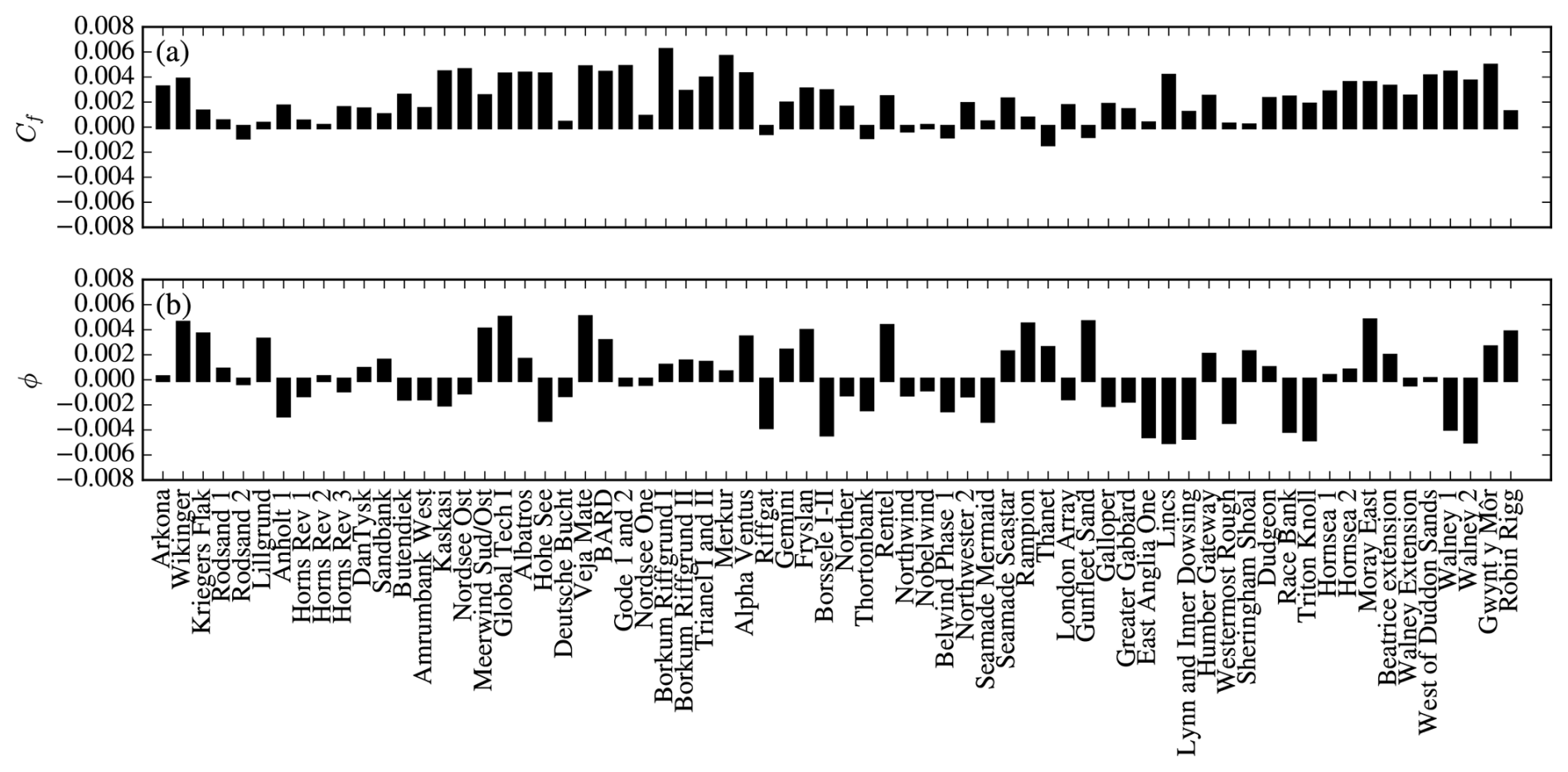
Figure A1 Difference between our model results and results of Simão Ferreira et al. (2026) Table S1 in terms of modeled wind farm capacity factor, C_f (a), and wind farm wind factor, ϕ (b).