Economic lifetime-aware wind farm control

We present the economic lifetime-aware formulation of wind farm control (WFC), a novel approach characterized by two key innovations with respect to the state of the art. First, the optimization is guided by an economic model of profit. By targeting profit instead of the more widely adopted power yield, the operational optimization considers not only the revenue generated by selling electricity (possibly at a variable price when operating on spot markets) but also the costs due to operation and maintenance (O&M). Second, since fatigue-induced damage is a finite-budget quantity, we explicitly consider that any effect on damage generated by a control action will leave more or less room to other control actions, a coupling that is neglected by current approaches that arbitrarily limit or penalize fatigue-inducing loads. To achieve this goal, the optimization is subjected to explicit constraints on lifetime, which ensure that the turbines in a farm and their components can indeed reach a desired goal duration. As for other optimization-based WFC approaches, the proposed method results in the offline calculation of optimal control set points for each turbine, which are scheduled and dispatched at run time in an open loop as functions of ambient conditions.

After introducing the economic lifetime-aware WFC approach, the paper analyzes two case studies. The first represents an idealized scenario characterized by a simplified set of environmental conditions, designed to demonstrate the behavior of the new control strategy and its impact on fatigue loads in conditions of very frequent waking. The second case features a more realistic small wind farm, with wind climate data derived from an existing meteorological mast. The benefits of the proposed methodology are highlighted by comparing it to alternative, previously published control strategies, which either ignore component damage or address fatigue loads in alternative, simplified ways. Results show that the lifetime-aware formulation always ensures the achievement of the desired lifetime targets, whereas methods that do not enforce such a condition may fail to do so. Additionally, the proposed method also results in the best economic performance, i.e., in the highest profit.

1 Introduction

1.1 Wind farm control beyond power

Most current wind farm control (WFC) strategies focus on increasing power generation (Meyers et al., 2022). However, this is only one of the several goals that may be targeted by the more general concept of optimal operation. In fact, a wind energy project sits in a complex dynamic environment and has various stakeholders. External factors, such as electricity market price or grid loads and transmission constraints, continuously evolve over time. These dynamics have an impact on the value of the wind farm power output being fed into the grid. For example, in some cases it pays off to extract maximum yield from the farm. In contrast, in other cases, generating less will be more convenient because the low electricity prices cannot offset the incurred costs.

Flow control strategies are designed to modify the inflow to the turbines in a farm. This can be obtained either by derating the turbines (called induction control), by misaligning them with respect to the wind (called wake steering), or by applying excitations meant to accelerate wake recovery (called wake mixing) (Meyers et al., 2022). However, every control action will affect the internal response of the farm, not only in terms of power but also in terms of the loading on the turbines. In turn, this affects their “health”, with a cascading direct influence on the overall asset lifetime and its repair and maintenance activities. Considering these factors and couplings, it seems hardly optimal to feed in maximum power to the grid at all times, and the successful optimization of a wind energy project requires a more holistic approach.

Some initial efforts at including fatigue in wind farm control have already been documented (Harrison et al., 2020b; Eguinoa et al., 2021; Dimitrov and Natarajan, 2021). Such control strategies typically try to restrict damage equivalent loads (DELs) by either setting a limiting value or by penalizing them through an additional objective. However, such choices can hardly lead to a clear understanding of the effects of control policies on lifetime. In fact, damage accrues over time, and therefore the control actions taken today – through the loading of the turbines – directly affect the room left for control actions that can be taken in the future. Thus, optimizing the operation of a wind farm over its lifetime cannot only rest on decisions based on present conditions or over short time horizons. Instead, one needs to consider the couplings between present and future actions.

More sophisticated approaches have been recently described that attempt to better express the trade-offs between fatigue and economic objectives that occur throughout the lifetime of an asset. Requate et al. (2023) introduced a framework for the optimal long-term planning of turbine operation that treats fatigue damage as a consumable budget. This approach actively distributes the damage budget along the operational life of the turbine to balance load reduction and energy output, demonstrating promise in reducing fatigue while maintaining performance. Similarly, Pettas (2024) developed an adaptive controller for wind turbines, tailored to reconcile fatigue and revenue goals. This approach uses variable power modes – including down-regulation and power boosting – alongside individual pitch control. A Gaussian process regression surrogate model is employed to capture trade-offs, enabling an optimization of the operational modes based on wind and price dynamics to maximize lifetime economic benefits.

Although clearly going in the direction of modeling the lifetime economics of wind assets, these studies are limited at the turbine level and do not consider the effects caused by wakes in a wind farm. As wake effects have been shown to significantly affect not only power capture but also structural loading (Kretschmer et al., 2021; Shaler et al., 2022; Reinwardt et al., 2021), the present work considers the problem at the farm – instead of the turbine – level.

1.2 Maximizing profit and ensuring a desired lifetime

Here we introduce a new form of WFC, termed economic lifetime-aware WFC. The formulation incorporates the current state of damage of the turbines – either provided by a digital twin or estimated from operational data – to compute control policies that optimize the long-term management of the wind farm. The problem is formulated as an optimization guided by an economic value function that expresses profit, i.e., the difference between revenue and cost.

Revenue is gained by producing power and selling it on the spot market at variable prices. However, in order to target profit, which is clearly a more complete economic indicator than revenue alone, it is necessary to account for the way turbines are operated. In fact, different operational strategies affect – through loads – the costs of operation and maintenance (O&M), in turn leading to loss of revenue due to downtime. Additionally, damage due to loads has also another effect on revenue and cost: when the lifetime of a component is affected, either the component must be replaced (which implies a cost for the spare part and its installation and a loss of revenue due to associated downtime), or the whole turbine must be dismantled, which leads again to a loss of revenue due to lost production caused by the shortened life. To account for such long-term effects on profitability, the optimization process proposed here is subject to constraints that ensure a target lifetime duration of selected turbine components is met.

The lifetime-aware economic optimization problem is solved in terms of control set points for each turbine. The type of control set points depends on the chosen operational modes, which may include induction control, wake steering, mixing, and possible combinations thereof. The proposed approach is demonstrated here using wake steering alone, but the method is general, and all other operational modes could be readily included.

Current WFC methods are based on the offline calculation of steady-state control set points, which are typically scheduled as functions of ambient conditions, such as wind speed, direction, and possibly other parameters in order to capture additional effects (Meyers et al., 2022). Since each ambient condition with its associated control action is independent from the others, a separate optimization is solved for each combination of scheduling parameters. The total number of necessary optimizations depends on the desired resolution (i.e., on the size of the bins used to discretize the parameters and the number of considered combinations). At run time, the current ambient conditions are detected and used to gauge from the precomputed set points the ones that need to be dispatched to the turbines in an open loop (Meyers et al., 2022). This method has the advantage of moving any computationally heavy optimization to the offline phase, while the run time execution is extremely fast and safe, because set points are sourced from a precomputed and verified pool. Dynamic (model predictive) approaches optimize performance over a prediction horizon, which might lead to improved performance compared to the just-described steady offline case (van den Broek et al., 2024). However, such methods require more complex dynamic flow models, shift the computationally intensive phase to the execution time, and generate new solutions at each call, which renders their verification for safety an additional challenge.

With our new formulation we aim to capture the long-term effects of control policies. In principle, this means that the economic optimization problem should be formulated over a potentially very long time horizon (the entire lifetime of the farm or a fraction of it). This would require the solution of a time-marching problem, which however would come at a potentially overwhelming computational cost. To make the problem tractable, we use an approach similar to the offline one described above. First, we bin the ambient parameters, and we count the frequencies of their combinations. Next, we solve the optimization problem that yields the control set points for each combination of binned parameters. The crucial distinction with the standard offline method described earlier is that now the solution is performed in one single shot, i.e., simultaneously considering all binned combinations with their respective frequencies. This clearly increases the computational cost because instead of many decoupled optimizations we now solve one single large one. However, this approach has the key advantage of coupling the effects of the control actions together. In fact, as we wrote earlier, a control action taken in some operating condition consumes some fraction of the lifetime and therefore changes the room left for other control actions that will be used in other operating conditions. By taking this coupling into account, we can include lifetime directly into the formulation (as a constraint), instead of working with DEL reductions or other unclear proxies.

Other advantages of the standard offline approach are retained here. In fact, while the solution may be expensive, it is still performed completely offline, and at run time set points are readily obtained from the precomputed ones based on the current ambient conditions. And here again, set points can be verified before they are actually deployed to the turbines, thereby guaranteeing their safety.

1.3 Application scenarios

As explained, our proposed WFC method departs from the current literature by (i) using a model of profit as an economic optimization objective and (ii) incorporating a desired lifetime as a constraint, thereby taking into account the room left by each control action for the others. While this paper highlights the combined use of these two innovations, it is important to realize that they can also be applied separately. In fact, if component damage is not a major concern (for instance, at a site with a mild environment relative to the turbine design limits), the lifetime constraint can be omitted while still using the economic value function to drive the optimization towards a maximization of profit. Eliminating the lifetime constraint reduces the computational cost (because independent – instead of coupled – optimizations can be performed for every combination of binned ambient parameters) while still offering a clearer optimization goal over existing formulations that blend power production and loads with arbitrary weighting factors (Harrison et al., 2020b).

This new economic lifetime-aware control framework can be used in different phases of a project. In a pre-deployment phase, a wind farm developer could use it to make informed decisions on the economic viability of various alternative operational scenarios. For instance, a developer could compare a shorter lifetime duration of the plant due to higher power capture (but also higher loading and hence higher O&M costs) followed by decommissioning vs. an extension of the plant lifetime beyond its initial intended duration thanks to a less aggressive capture and less loading. In a second phase, once an optimal life management strategy has been selected, the wind farm operator can deploy the corresponding lifetime-aware controller to operate the turbines in the chosen profit-optimal way while ensuring that the specified lifetime goals are met.

1.4 Scope and organization of the work

The economic model of profit used here is simple, one of its main limitations being the crude link between the effects of loads and O&M costs. While this is due to the limited open literature existing on this important – although little investigated – topic, it is clear that better models, such as those surely available at several major companies, could be readily used within this approach without significant modifications.

An experimental validation of the proposed WFC methodology was recently conducted by wind tunnel tests (Braunbehrens et al., 2024). The experiment involved three model turbines in a boundary layer wind tunnel, where a turntable was used to simulate dynamic variations in wind direction. The control strategy, based on wake steering, was synthesized using power and damage estimators. The proposed strategy was compared to conventional greedy operation and the classical maximum power strategy. Results showed how the new control approach not only improved the economic performance of the wind farm but also ensured operation over the desired lifetime. In this paper, we develop a more detailed description of the economic lifetime-aware WFC formulation than the one of Braunbehrens et al. (2024), and we demonstrate the new method in a simulation environment.

The rest of this paper is organized as follows. The proposed approach is presented in Sect. 2. This is followed in Sect. 3 by a detailed description of the optimization framework that, with its supporting models and tools, enables the calculation of the profit-optimal control laws. Next, in Sect. 4 the economic lifetime-aware WFC method is applied to two case studies, considering various performance indicators, including power, loads, lifetime duration, and profit. Results are compared to some alternative WFC formulation sourced from the recent literature. Finally, conclusions and key findings are discussed in Sect. 5.

2 Lifetime-aware wind farm operational optimization

2.1 Operational optimization for profitability

We consider the problem of optimizing the way a wind farm is operated in order to maximize its profitability.

Profit expresses the trade-off between control actions aimed at increasing the revenue generated by power yield and those designed to mitigate the economic cost of fatigue damage (Wilkinson et al., 2010; Scheu et al., 2017). In order to optimize for profit, a suitable economic model is required. The economic model builds on a physical model expressing the effects of the control actions on the flow within the farm, and hence on power capture. In turn, power yields revenue, gained by selling electricity. The same flow model informs a load model that provides the fatigue loads on the turbines, whose accumulation finally yields damage. In turn, damage enables the calculation of O&M costs and lifetime duration, the latter again affecting revenue.

Section 3 explains how these various models can be formulated and connected together in order to enable the operational optimization of the farm for maximum profitability.

2.2 Operational time horizon

The operational optimization is performed over a certain time horizon.

In a first scenario, this temporal horizon is unknown. In other words, the solution of the operational optimization yields the way the turbines should be operated, but also the length of time over which the wind farm should be run. Extending the operation beyond that optimal duration would result in a smaller profit, for example because of excessive costs due to the aged turbines, because replacing them with more modern machines would be more economically profitable, or for various other reasons.

In a second scenario, the operational optimization of the wind farm is defined over a known desired temporal horizon. In this case, for example, a developer might want to ensure that a new wind farm is operated with maximum profit for a duration of at least X years. Another example might be an operator that owns a farm that has been running for Y years and now wants to optimize the economic performance of that farm for the next Z years.

This work considers this second scenario: we want to ensure that turbines in a farm are operated in a profit-optimal way for a desired period of time without exceeding a predefined damage threshold. This threshold may represent the design lifetime of the turbines or a desired fraction of the remaining useful life, depending on the scenario (see the Results and discussion section for an example). Clearly, the ability to reach a desired duration has economic implications, as failure to do so would result in revenue losses due to the reduced lifespan. Published WFC formulations cannot guarantee that this objective is met. The present formulation tries to fill this gap.

2.3 Accounting for lifetime in operational optimization

Although ensuring a desired lifetime has a clear economic advantage, it also drastically complicates the problem of designing a controller capable of achieving such a goal.

To understand this aspect of the problem, consider a standard wind farm controller based on the offline optimization of steady-state set points and their subsequent online, open-loop dispatch to the turbines (Campagnolo et al., 2020; Göçmen et al., 2022; Howland et al., 2019). Ambient conditions are characterized by combinations of parameters such as wind speed U, direction Γ, turbulence intensity (TI) I, and possibly others. Such conditions have an effect on the wakes that couple the turbines together in a farm. To account for such effects, the atmospheric parameters are first discretized into bins and combined to create a finite set of discrete ambient conditions. Next, set points are calculated for each one of these discrete ambient conditions. Since there are no couplings among the different conditions and among the associated control actions, multiple independent calculations of the set points can be performed.

On the other hand, a different approach is necessary when lifetime needs to be precisely accounted for. This is due to the fact that fatigue damage in a turbine component accumulates in a complex way over its lifespan, influenced by all encountered ambient conditions and all performed control actions. Consequently, the damage accumulated at a given time in some given wind condition directly affects the remaining operational life of the turbine.

2.4 Lifetime-aware operational optimization in the time domain

As a result of this coupling among actions and over time, the design of a fatigue-aware wind farm control policy cannot be performed for separate conditions. Instead, it is formulated as an optimal control problem (Betts, 2010) in the time domain t defined over a desired lifetime horizon T, which is expressed as

$$\begin{array}{}\text{(1a)}& \underset{\mathit{u}\left(t\right)}{max}\underset{t\in T}{\int }\left(\text{Revenue}\left(\mathit{u}\right(t),t)-\text{Cost}\left(\mathit{u}\right(t),t)\right)\mathrm{d}t,\end{array}$$

subject to

$$\begin{array}{}\text{(1b)}& {\displaystyle }& {\displaystyle }{D}_i^c\left(T\right)\le D_{\mathrm{ref}}^c\forall i\in N,\forall c\in C,\text{(1c)}& {\displaystyle }& {\displaystyle }{\mathit{u}}_i^{min}\le {\mathit{u}}_i\left(t\right)\le {\mathit{u}}_i^{max}\forall i\in N.\end{array}$$

In the open-horizon scenario described before, the duration T is an unknown of the problem, together with the control actions u(t). Although this problem is clearly very relevant for developers and/or operators, here we study the simpler problem where T is given, and we call it the goal (desired) duration. As is apparent in the following, even this simpler problem is complex and expensive, and therefore it is the sole focus of this work.

2.4.1 Optimization objective

The optimization problem expressed by Eq. (1a)–(1c) accounts for the economic value accrued through power generation, as expressed by the Revenue(⋅) function, but also for the economic cost incurred through maintenance activities and lost lifetime, as quantified by the Cost(⋅) function. Profit is the difference between these two quantities.

Notice that in Eq. (1a) revenue and cost depend explicitly on time t because of time discounting, which is used to estimate the present worth of future cash flows. The role of discounting in economic WFC is discussed in Sect. 3.4.3.

2.4.2 Optimization unknowns

Revenue and cost depend on the control actions $\mathit{u}\left(t\right)=\left[{\mathit{u}}_{\mathrm{1}}\left(t\right),\mathrm{\dots },{\mathit{u}}_i\left(t\right),\mathrm{\dots },{\mathit{u}}_N\left(t\right)\right]$, where u_i(t) is the vector containing the control set points (yaw, induction, etc.) of turbine i of the N turbines in the farm.

The control actions u(t) represent the functional unknowns of problem (1a)–(1c), and they depend on the time-variable ambient conditions W_a(t), i.e.,  u(t)=u(W_a(t)). In this work, ambient conditions are represented by the combination of wind speed, direction, and turbulence intensity: ${\mathit{W}}_{\mathrm{a}}\left(t\right)=\left\{U\left(t\right),\mathrm{\Gamma }\left(t\right),I\left(t\right)\right\}$.

The bound constraint Eq. (1c) ensures that the set points u_i(t) for each turbine i remain within desired lower (${\mathit{u}}_i^{min}$) and upper (${\mathit{u}}_i^{max}$) bounds.

2.5 Lifetime constraint

The optimization problem is subjected to the lifetime constraint expressed by Eq. (1b), which ensures that the damage $D_i^c\left(T\right)$ of component c in the set of components C for turbine i at the end of the desired lifetime T does not exceed the damage threshold $D_{\mathrm{ref}}^c$. This threshold is an appropriate damage limit, which includes the necessary safety factors. Clearly, there are several options for determining this limit. For instance, $D_{\mathrm{ref}}^c$ could be set to the design limit, allowing the component to be utilized up to its maximum designed capacity. Alternatively, one might leave a damage margin, ensuring that the component has a second life. Despite the various possible scenarios, the underlying concept of this approach is to maintain control over damage accumulation while pursuing a specific goal. Achieving this goal over a desired duration would not be possible without an explicit constraint that ensures that the duration will be met.

If the constraint expressed by Eq. (1b) is violated, the problem is infeasible. This means that it is not possible to operate the farm for the time duration T without exceeding the damage threshold. In contrast, if the constraint expressed by Eq. (1b) is satisfied, and

$$\begin{array}{}\text{(2)}& D_i^c\left(T\right)-D_{\mathrm{ref}}^c>\mathrm{0}\forall i\in N,\forall c\in C,\end{array}$$

then this means that the farm can be operated over the entire duration T, and some damage margin is still left. Therefore the farm could in principle be run for a longer period of time than the required T. By knowing the initial damage at time t=0 and the remaining margin at time t=T, the point in time when the damage threshold is reached can be estimated by linear extrapolation. It should be noted that the optimization is not performed over this extra time duration. However, the quantification of the extra profit that in principle could be achieved can be readily obtained by computing the extra revenue and cost accrued over this extended lifetime.

To conclude the discussion on the lifetime constraint, a distinction should be made between a replaceable and an irreplaceable component (e.g., the tower). A replaceable component requires some cost and downtime, after which the turbine goes back into operation. An irreplaceable component, on the other hand, implies that the turbine lifetime is exhausted, and the machine has to be dismantled. Although both situations should be taken into account for a general formulation, only the case of irreplaceable components is considered here to shorten the notation and to ease the implementation. In the applications presented later, the blades and the tower are treated as components, even the blades, for simplicity, being considered irreplaceable.

2.6 Reformulation from the time domain to probability distributions

A time series implementation of the problem expressed by Eq. (1a)–(1c) would require (i) providing a time series of atmospheric parameters over the lifetime T and (ii) solving the optimization problem for the corresponding time series of control set points u(t). Today this is clearly unfeasible, as it would imply overwhelming computational costs. In addition, this approach would also be wasteful, as similar combinations of atmospheric parameters would appear over and over again during the optimization horizon.

To address this hurdle, the atmospheric parameters (speed, direction, TI, etc.) are first discretized into bins. Next, time series of the parameters are converted into discrete sets of ambient conditions ${\mathit{W}}_{\mathrm{a}}^{\text{bin}}$, each being represented by a combination of the binned parameters. Counting its occurrences, each ambient condition is associated with its probability $f_{\mathrm{a}}^{\text{bin}}$. To account for the temporal variability in the wind climate, different probabilities $f_{\mathrm{a},y}^{\text{bin}}$ can be used for each epoch y (an epoch being a certain duration of time, for example 1 year), with y∈Y, Y being the number of epochs in the time horizon T.

Next, the control set points of each turbine u_i, instead of depending on time t, are assumed to depend on the discrete ambient conditions, i.e., ${\mathit{u}}_i\left({\mathit{W}}_{\mathrm{a}}^{\text{bin}}\right)$, and therefore for the whole farm $\mathit{u}\left({\mathit{W}}_{\mathrm{a}}^{\text{bin}}\right)=\left[{\mathit{u}}_{\mathrm{1}}\left({\mathit{W}}_{\mathrm{a}}^{\text{bin}}\right),\mathrm{\dots },{\mathit{u}}_N\left({\mathit{W}}_{\mathrm{a}}^{\text{bin}}\right)\right]$. Finally, the time-dependent cost function appearing in Eq. (1a) can be approximated using combinations of binned parameters as

$$\begin{array}{}\text{(3)}& \begin{array}{rl}\underset{t\in T}{\int }& \left(\text{Revenue}\left(\mathit{u}\right(t),t)-\text{Cost}\left(\mathit{u}\right(t),t)\right)\mathrm{d}t\\ & \approx \sum _{y\in Y}\sum _{\mathrm{bin}\in \text{Bins}}{f}_{\mathrm{a},y}^{\text{bin}}\left(\text{Revenue}\left(\mathit{u}\right({\mathit{W}}_{\mathrm{a}}^{\text{bin}}),y)\right.\\ & \left.-\text{Cost}\left(\mathit{u}\right({\mathit{W}}_{\mathrm{a}}^{\text{bin}}),y)\right).\end{array}\end{array}$$

Notice that here we are assuming that the same ambient condition will always trigger the same control response. While this seems to be reasonable, such an assumption does not necessarily hold for the time domain problem Eq. (1a)–(1c). While it would be possible to allow for this extra freedom even here, by assuming a different set of control set points for each epoch, this approach is not pursued further because of its extra cost. A further discussion on this aspect of the formulation is developed in Sect. 3.4.3 with reference to time discounting.

By moving from the time domain to probability distributions of discrete ambient conditions, the problem expressed by Eq. (1a)–(1c) is reformulated as

$$\begin{array}{}\text{(4a)}& \begin{array}{rl}\underset{\mathit{u}}{max}\sum _{y\in Y}\sum _{\mathrm{bin}\in \text{Bins}}& f_{\mathrm{a},y}^{\text{bin}}\left(\text{Revenue}\left(\mathit{u}\right({\mathit{W}}_{\mathrm{a}}^{\text{bin}}),y)\right.\\ & \left.-\text{Cost}\left(\mathit{u}\right({\mathit{W}}_{\mathrm{a}}^{\text{bin}}),y)\right),\end{array}\end{array}$$

subject to

$$\begin{array}{}\text{(4b)}& {\displaystyle }& {\displaystyle }{D}_i^c\left(T\right)\le D_{\mathrm{ref}}^c\forall i\in N,\forall c\in C,\text{(4c)}& {\displaystyle }& {\displaystyle }{\mathit{u}}_i^{min}\le {\mathit{u}}_i\left({\mathit{W}}_{\mathrm{a}}^{\text{bin}}\right)\le {\mathit{u}}_i^{max}\forall i\in N,\forall \text{bin}\in \text{Bins}.\end{array}$$

The unknowns of the reformulated problem are the turbine discrete set points for each ambient condition $\mathit{u}\left({\mathit{W}}_{\mathrm{a}}^{\text{bin}}\right)$. As for the original problem, even the new one is subjected to damage (Eq. 4b) and bound (Eq. 4c) constraints.

This reformulation drastically decreases the computational cost of the problem, as one does not solve anymore for time series of control set points, but for control set points for each combination of binned atmospheric parameters, as commonly done in standard power-boosting WFC.

As for this standard approach, even here the optimization is performed offline, while online – once the current ambient conditions have been determined – the corresponding set points are first sourced from the pre-computed solution and then dispatched in an open loop to the turbines in the farm (Campagnolo et al., 2020; Göçmen et al., 2022; Howland et al., 2019). This means that all expensive calculations are relegated to the offline case and that the set points can be verified for safety before being implemented in the field.

2.7 Reference control formulations

In addition to the proposed formulation, in the following referred to as “max-profit”, another five WFC strategies are used in Sect. 4 for comparing in various scenarios the performance of alternative control strategies. We consider greedy control, power-boosting control, and three load-aware formulations that account for component fatigue. Except for the greedy case, all formulations use wake steering, subject to the same yaw misalignment bounds. A brief description of each of these WFC strategies is provided below.

1. Greedy. This formulation represents the standard operational mode for most existing wind farms. Following this approach, each turbine in the farm operates independently from the others to maximize its own power capture, by orienting its rotor to face the local wind direction. This formulation serves as a baseline for comparison.

2. Max-power. This formulation corresponds to the classical annual energy production (AEP) maximization (or power boosting) by wake steering (Meyers et al., 2022). The optimization problem is formulated as

   $$\begin{array}{}\text{(5a)}& \underset{\mathit{u}}{max}\sum _{y\in Y}\sum _{\mathrm{bin}\in \text{Bins}}{f}_{\mathrm{a},y}^{\text{bin}}\sum _{i=\mathrm{1}}^N{P}_i\left(\mathit{u}\right({\mathit{W}}_{\mathrm{a}}^{\text{bin}}\left)\right),\end{array}$$

   subject to

   $$\begin{array}{}\text{(5b)}& {\mathit{u}}_i^{min}\le {\mathit{u}}_i\left({\mathit{W}}_{\mathrm{a}}^{\text{bin}}\right)\le {\mathit{u}}_i^{max}\forall i\in N,\forall \text{bin}\in \text{Bins}.\end{array}$$

   The cost function represents the overall farm power output for all ambient conditions with their probabilities during the lifetime duration. Maximizing this quantity corresponds to maximizing revenue for a fixed price of electricity.

3. Load-constrained. The formulation targets revenue while limiting loading on the turbine components, and it is adapted from the discussions in TotalControl (2022b) and Eguinoa et al. (2021). The optimization problem is expressed as

   $$\begin{array}{}\text{(6a)}& \underset{\mathit{u}}{max}\sum _{y\in Y}\sum _{\mathrm{bin}\in \text{Bins}}{f}_{\mathrm{a},y}^{\text{bin}}\text{Revenue}\left(\mathit{u}\right({\mathit{W}}_{\mathrm{a}}^{\text{bin}}),y),\end{array}$$

   subject to

   $$\begin{array}{ll}{\displaystyle }& {\displaystyle }{D}_i^c\left(\mathit{u}\right({\mathit{W}}_{\mathrm{a}}^{\text{bin}}\left)\right)\le \mathbb{K}\underset{i}{max}{D}_i^c\left({\mathit{W}}_{\mathrm{a}}^{\text{bin}}\right)\forall i\in N,\\ \text{(6b)}& {\displaystyle }& {\displaystyle }\forall c\in C,\forall \text{bin}\in \text{Bins},\text{(6c)}& {\displaystyle }& {\displaystyle }{\mathit{u}}_i^{min}\le {\mathit{u}}_i\left({\mathit{W}}_{\mathrm{a}}^{\text{bin}}\right)\le {\mathit{u}}_i^{max}\forall i\in N,\forall \text{bin}\in \text{Bins}.\end{array}$$

   The damage limit for a given component c is defined as the maximum damage observed across all turbines in the baseline greedy case, scaled by a factor 𝕂. This parameter represents the safety factor typically applied during the turbine design phase to account for additional loading during operation and all other uncertainties. The damage limit is set individually for each ambient wind condition bin ${\mathit{W}}_{\mathrm{a}}^{\text{bin}}$ within the full set of wind conditions W_a.

4. Load-balance. This formulation balances power production and loading, following the discussions in Harrison et al. (2020a), Bossanyi (2018), and Kanev et al. (2018). The optimization problem is expressed as

   $$\begin{array}{}\text{(7a)}& \begin{array}{rl}\underset{\mathit{u}}{max}& \left({\mathbb{W}}_P\sum _{y\in Y}\sum _{\mathrm{bin}\in \text{Bins}}{f}_{\mathrm{a},y}^{\text{bin}}\sum _{i=\mathrm{1}}^N{P}_i\right(\mathit{u}\left({\mathit{W}}_{\mathrm{a}}^{\text{bin}}\right))\\ & -\sum _{c\in C}{\mathbb{W}}_D^c\sum _{\mathrm{bin}\in \text{Bins}}\underset{i}{max}{D}_i^c\left(\mathit{u}\right({\mathit{W}}_{\mathrm{a}}^{\text{bin}}\left)\right)),\end{array}\end{array}$$

   subject to

   $$\begin{array}{}\text{(7b)}& {\mathit{u}}_i^{min}\le {\mathit{u}}_i\left({\mathit{W}}_{\mathrm{a}}^{\text{bin}}\right)\le {\mathit{u}}_i^{max}\forall i\in N,\forall \text{bin}\in \text{Bins}.\end{array}$$

   The cost function is composed of two terms. The first represents the total power generated by the wind farm. The second term is designed to prioritize turbines with a higher available fatigue budget, stressing them more than those with greater accumulated damage, thereby ensuring a more balanced load distribution throughout the farm. To achieve this effect, function $\underset{i}{max}{D}_i^c$ selects the maximum damage accrued across all turbines for a given component c. The weight parameters 𝕎_P and ${\mathbb{W}}_D^c$ are used to adjust the relative importance of the two terms in the objective function.

5. Lifetime-revenue. This formulation is a modification of the proposed one, where the optimization objective targets only revenue instead of profit, and is expressed as

   $$\begin{array}{}\text{(8a)}& \underset{\mathit{u}}{max}\sum _{y\in Y}\sum _{\mathrm{bin}\in \text{Bins}}{f}_{\mathrm{a},y}^{\text{bin}}\text{Revenue}\left(\mathit{u}\right({\mathit{W}}_{\mathrm{a}}^{\text{bin}}),y),\end{array}$$

   subject to

   $$\begin{array}{}\text{(8b)}& {\displaystyle }& {\displaystyle }{D}_i^c\left(T\right)\le D_{\mathrm{ref}}^c\forall i\in N,\forall c\in C,\text{(8c)}& {\displaystyle }& {\displaystyle }{\mathit{u}}_i^{min}\le {\mathit{u}}_i\left({\mathit{W}}_{\mathrm{a}}^{\text{bin}}\right)\le {\mathit{u}}_i^{max}\forall i\in N,\forall \text{bin}\in \text{Bins}.\end{array}$$

3 Optimization framework

This section describes the optimization framework that was developed to compute the optimal control set points for a wind farm according to the proposed economic lifetime-aware WFC strategy. Elements of this framework are also used for implementing the alternative strategies described in Sect. 2.7. An overview of the framework, including its underlying models, is depicted in Fig. 1. The framework takes as input binned site-specific wind conditions ${\mathit{W}}_{\mathrm{a}}^{\text{bin}}$ with their probabilities of occurrence $f_{\mathrm{a}}^{\text{bin}}$ and generates optimal control schedules $\mathit{u}\left({\mathit{W}}_{\mathrm{a}}^{\text{bin}}\right)$ for all turbines in the form of look-up tables.

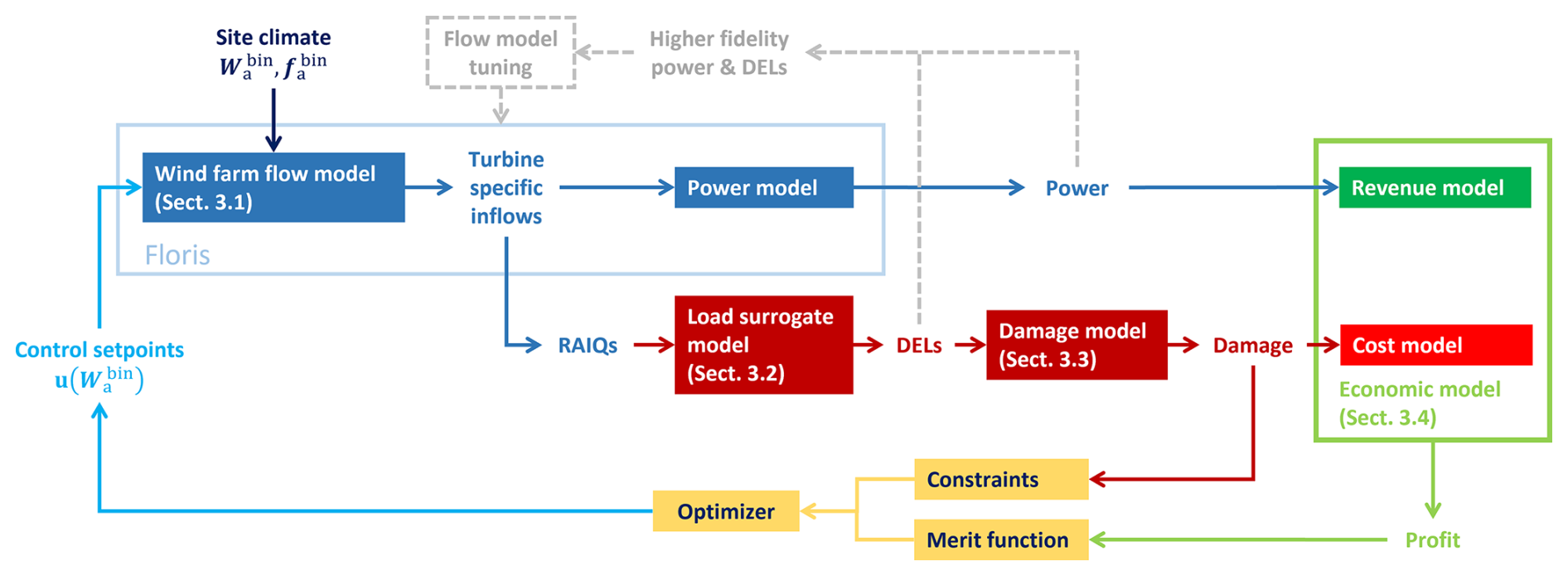
Figure 1 Graphical visualization of the computational framework supporting the implementation of the economic lifetime-aware WFC strategy.

The model toolchain consists of several components: a fast wind farm engineering flow model (Sect. 3.1), a fatigue load surrogate model (Sect. 3.2), a damage estimation model (Sect. 3.3), and an economic model of profit (Sect. 3.4).

The upper branch of the toolchain follows established research and industry practices for estimating the power production of a wind farm (Lee and Fields, 2021), which is then converted into revenue by the economic model. The central branch tackles the more complex task of estimating the impact of the operational strategy on the fatigue of the turbine components. To this end, for each turbine, its rotor inflow conditions are first mapped into DELs, which are then aggregated to estimate damage. In turn, the accumulated damage is used to calculate the associated maintenance costs. By combining the upper branch (revenue) and the central branch (cost), the framework generates the merit function and constraint that define the optimization problem. An optimization algorithm is used to solve the resulting constrained maximization, which finally yields the control set points, as shown in the lower branch of the figure.

Each individual model block is discussed in the following.

3.1 Wind farm flow model

The flow model simulates wake interactions within the wind farm, first mapping the ambient site inflow W_a to turbine-specific inflows and then estimating the production of each turbine by a power model. Steady-state engineering wake models offer a suitable compromise between accuracy and computational cost, which is one of the main reasons behind their widespread use in industry and academia (Porté-Agel et al., 2019). Furthermore, their tunable parameters allow for site-specific calibration. The present study uses the open-source toolbox FLORIS (NREL, 2022). Real-world wind farm flow fields are influenced by additional factors such as terrain-induced effects and interactions between the farm and the atmospheric boundary layer. Models of these effects are being developed (Stipa et al., 2024) or can be learned, augmented, and/or tuned from operational data (Braunbehrens et al., 2023).

Figure 2a depicts the hub height flow field for an exemplary two-turbine cluster for ${\mathit{W}}_{\mathrm{a}}=\left\{\mathrm{8}{\mathrm{m}\mathrm{s}}^{-\mathrm{1}},\mathrm{275}\mathit{°},\mathrm{12}\mathit{\%}\right\}$. The flow field predicted by the model at each turbine rotor disk is first used, through a turbine-specific power model, to compute the power output of each turbine and then of the whole farm. As shown in the upper branch of Fig. 1, power is then fed into the economic model to estimate revenue. In the lower branch, the local wind speed and turbulence intensity conditions generated by the flow model at each specific turbine are provided as input to a surrogate load model (see Sect. 3.2).

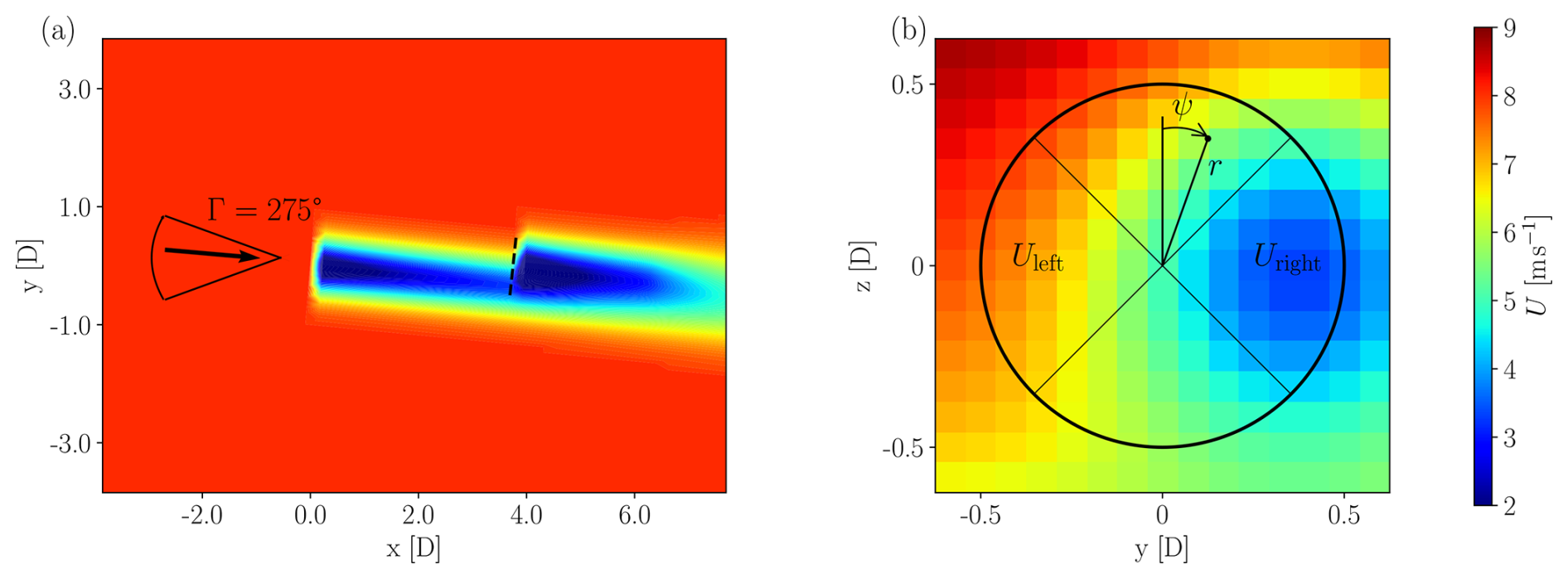
Figure 2 Streamwise velocity field for a two-turbine cluster, modeled with FLORIS. (a) Horizontal plane at hub height. The indicated sector visualizes the wind direction sweep used later in Sect. A1. (b) Distribution of the longitudinal flow speed just in front of the downstream turbine (see dashed line in panel a). The figure includes the outline of the rotor and its left and right quadrants used by the surrogate load model (see Sect. 3.2).

Figure 2b illustrates the streamwise velocity field just upstream of the rotor of the second turbine, as extracted from FLORIS. In this work we use the Gaussian wake deficit model (Bastankhah et al., 2014) because of its ability to capture the non-uniform distribution of the flow speed in partial-wake impingements, as the one shown in the figure. The model includes the tuning parameters k_α, k_β, k_a, and k_b that, in pairs, control the far-wake onset and decay, respectively. In contrast, the simpler Jensen velocity model provides only for a cruder representation of the inflow due to the assumption of a top-hat profile (Katic et al., 1987); it was found that such level of approximation is not accurate enough when loading needs to be computed.

Wake-added turbulence is another important parameter for an accurate estimation of loading. In particular, the model by Crespo and Hernandez (1996) was found not to be sufficiently accurate in partial-wake situations. Similarly to the Jensen model in the just-discussed case of wake deficit, this is primarily due to the overly simplified, top-hat-like profile of turbulence assumed by the Crespo–Hernandez model. To address this limitation, we implemented the model proposed by Ishihara and Qian (2018), which features an axisymmetric double-Gaussian TI profile.

Additionally, the model equations were enhanced by making the parameters k_G, k_σ, and k_r0 tunable, which respectively allow for the calibration of the maximum added TI, of the profile width, and of the peak distance.

The “wind farm as a sensor” method was employed for the simultaneous calibration of the parameters of the flow model (Braunbehrens et al., 2023, 2024), as explained more in detail in the next section.

3.2 Load model

Following the lower branch in Fig. 1, the load model is tasked with mapping turbine-specific inflow conditions to fatigue loads, which in turn enable the estimation of turbine lifetime and maintenance costs. As surrogate models are relatively new, the present section gives a brief review of the formulation that was used here.

The load surrogate model predicts short-term DELs for monitored components (load channels), which are then used to calculate damage. Loads depend primarily on the local inflow conditions at the rotor disk of a turbine. As shown in Fig. 2b, impinging wakes significantly alter the characteristics of the incoming flow field. Additionally, self-loads are influenced by the control actions performed by a turbine. For example, misaligning a turbine to steer its wake can affect the loading of its various components to a different degree (Damiani et al., 2018).

Aeroservoelastic simulations are required to estimate DELs at the component level. To include the effects of wakes, here we use FAST.Farm (Jonkman and Shaler, 2021), a tool that computes the generation of wakes with their meandering and evolution (Larsen et al., 2007) in a turbulent flow field, here based on the Kaimal model (Jonkman, 2016), together with the impingement of the wakes on downstream wind turbines. We use the extension proposed by Kretschmer et al. (2021) to provide a more accurate description of wake-added turbulence. Both wake-shedding and wake-impinged wind turbines are modeled with the aeroservoelastic simulator OpenFAST (NREL, 2023).

However, running these simulations within an optimization, as in the present case, is clearly computationally infeasible.

In fact, the complexity and cost of the simulations needed to predict DELs have led to an increasing interest of the recent literature in load surrogates. These are fast models that predict DELs by “interpolating” within a large database of pre-computed results. While the generation of the database may require a very substantial number of complex simulations and therefore a high computational effort, the sourcing from this substantial data pool of the DELs that are relevant to a given condition can be done very efficiently at run time. Hence, load surrogates are key for the inclusion of loads in any situation where one needs to compute DELs in a large number of different conditions, as for the present control optimization.

Several approaches for load surrogates have been proposed in the literature (Dimitrov et al., 2018; Mendez Reyes et al., 2019; Bossanyi, 2022; Shaler et al., 2022; Liew et al., 2024). However, these methods are often layout-specific, requiring dedicated training for any given wind farm, or fail to account for the effects of control actions on self-induced loads and those experienced by downstream turbines.

The present work adopts the load surrogate approach proposed by Guilloré et al. (2024). This surrogate is location-agnostic, in the sense that a single model can predict loads at any pad within an arbitrary wind farm. This is obtained by mapping, through a neural network, some selected features of the inflow at the turbine rotor disk with the DELs experienced by chosen components. Since the mapping is between the inflow at a turbine and the DELs of that same turbine, it is not necessary to know where the turbine is located, but only its wind inflow. The present surrogate is also control-oriented, in the sense that the effects of control actions (yaw misalignment or down-regulation) on self-fatigue are accounted for.

3.2.1 Inflow characterization

The description of the turbine inflow that serves as input to the load surrogate has crucial importance. Simply using the fully resolved velocity field generated in FAST.Farm of other similar mid- or high-fidelity models is not a practical choice, as machine learning models tend to “learn the noise” present in the turbulence. Therefore, in addition to requiring a very large number of inputs, the model would perform well on the training set but poorly on test data (Guilloré et al., 2024). To avoid this overfitting problem, it is necessary to define suitable reduced-order quantities that minimize noise while retaining enough informational content to adequately characterize the flow field from the point of view of its effects on DELs.

Additionally, the inflow description must account for the fact that two flow models of different fidelity are used during two different steps in the process. During the generation of the dataset later used to train the surrogate, a mid-fidelity dynamic wake meandering model, here implemented in FAST.Farm (Jonkman and Shaler, 2021), simulates in the time domain the wake evolution caused by ambient eddies. In contrast, the optimization framework used to synthesize the farm control laws is necessarily based on a computationally cheaper low-fidelity, steady-state engineering flow model, here implemented in FLORIS (NREL, 2022). Although both models share some similarities, there is an unavoidable mismatch between the flow fields generated by the steady-state engineering model and the mid-fidelity dynamic one.

This problem is addressed here as follows.

First, the default Crespo–Hernandez (Crespo and Hernandez, 1996) top-hat wake-added turbulence model in FLORIS was replaced with the Ishihara and Qian (2018) model because of the similarity of its double-peaked TI with the model implemented in FAST.Farm (Jonkman and Shaler, 2021).

Second, to improve the match between the engineering steady-state model and the dynamic one, all free model parameters of the former were calibrated using the dataset generated with the latter. The calibration of the parameters was obtained with the “wind farm as a sensor” method, which uses a maximum likelihood approach to identify corrections to the baseline values of the parameters (Braunbehrens et al., 2023). This model tuning is obtained as the optimization of a cost function combining the residuals for power and rotor-average TI on each rotor disk in the farm for all ambient conditions of interest (see gray branch in Fig. 1).

Third, we use a slightly modified version of the inflow characterization, compared to the one presented in Guilloré et al. (2024). Instead of relying on sector-averaged inflow quantities, this work utilizes three rotor-averaged inflow quantities (RAIQs), namely the rotor-averaged wind speed (RAWS), the rotor-averaged turbulence intensity (RATI), and the rotor-averaged horizontal shear (RAHS). This approach simplifies the complex local inflow across the rotor by reducing it to only three representative variables. Although the sector-averaged inflow quantities of Guilloré et al. (2024) offer an improved accuracy, the present, simpler approach still contains sufficient information to capture DELs and their trends.

The RAWS is defined as the mean wind speed across the rotor disk, i.e.,

$$\begin{array}{}\text{(9)}& \text{RAWS}=\underset{\mathrm{0}}{\overset{\mathrm{2}\mathit{\pi }}{\int }}\underset{\mathrm{0}}{\overset{R}{\int }}U(r,\mathit{\psi })\mathrm{d}r\mathrm{d}\mathit{\psi }.\end{array}$$

Here, U(r,ψ) is the local wind speed at a given point, with r and ψ being the radial and azimuthal coordinates, respectively. Similarly, the RATI is defined as the mean TI across the rotor disk and is written as

$$\begin{array}{}\text{(10)}& \text{RATI}=\underset{\mathrm{0}}{\overset{\mathrm{2}\mathit{\pi }}{\int }}\underset{\mathrm{0}}{\overset{R}{\int }}I(r,\mathit{\psi })\mathrm{d}r\mathrm{d}\mathit{\psi },\end{array}$$

where I(r,ψ) is the local TI at a given point on the inflow plane. Finally, the RAHS represents the heterogeneity of wind speed across the rotor disk in the lateral direction. RAHS is particularly useful for characterizing cases of full or partial-wake overlap. The definition is based on Bottasso et al. (2018) and Schreiber et al. (2020), using the left and right quadrants of the rotor disk, as visualized in Fig. 2b. The left and right quadrant-equivalent wind speeds can be calculated as

$$\begin{array}{}\text{(11a)}& {\displaystyle }{U}_{\mathrm{right}}=\underset{\mathit{\pi }/\mathrm{4}}{\overset{\mathrm{3}/\mathrm{4}\mathit{\pi }}{\int }}\underset{\mathrm{0}}{\overset{R}{\int }}U(r,\mathit{\psi })\mathrm{d}r\mathrm{d}\mathit{\psi },\text{(11b)}& {\displaystyle }{U}_{\mathrm{left}}=\underset{\mathrm{5}/\mathrm{4}\mathit{\pi }}{\overset{\mathrm{7}/\mathrm{4}\mathit{\pi }}{\int }}\underset{\mathrm{0}}{\overset{R}{\int }}U(r,\mathit{\psi })\mathrm{d}r\mathrm{d}\mathit{\psi }.\end{array}$$

The horizontal shear coefficient RAHS is estimated under the assumption of a linear variation in wind speed along the lateral direction. It is further assumed that the quadrants sample the inflow at $\pm \mathrm{2}/\mathrm{3}$ of the rotor radius, as described by Bottasso et al. (2018) and Schreiber et al. (2020). Thus, RAHS can be calculated as

$$\begin{array}{}\text{(12)}& \text{RAHS}={\displaystyle \frac{\mathrm{3}}{\mathrm{2}}}{\displaystyle \frac{U_{\mathrm{right}}-U_{\mathrm{left}}}{U_{\mathrm{right}}+U_{\mathrm{left}}}}.\end{array}$$

An example of the behavior of these three RAIQs is illustrated in Appendix A1 with reference to a wind direction sweep for the two turbines of Fig. 2.

3.2.2 Damage equivalent loads

Given a load time series at a selected component location obtained with the FAST.Farm simulations, DELs are estimated for a 10 min time window using the rainflow counting algorithm and the classical formula

$$\begin{array}{}\text{(13)}& \text{DEL}={\left({\displaystyle \frac{{\sum }_i\left(n_i{L}_i^m\right)}{N_{\mathrm{eq}}}}\right)}^{\frac{\mathrm{1}}{m}},\end{array}$$

as described for example in Sutherland (1999) and in IEC 61400-1 (2019). Here, n_i is the number of load cycles of amplitude L_i, N_eq is the equivalent number of cycles (taken conventionally to be equal to 2×10⁶ cycles over a lifetime of 20 years), and m is the Wöhler exponent of the S–N curve of the component material. Typical values for the material constants are m=10 for the polymer of the blades and m=4 for the steel of the tower (Sutherland, 1999; IEC 61400-1, 2019).

In this work, we consider two load channels, one at the blade root and the other at the tower base. Both are obtained by projecting the bending moment components (flapwise and edgewise for blades, fore–aft and side–side for the tower) along the maximum damage direction. See Guilloré et al. (2024) for details on this projection.

3.2.3 Surrogate load model

After having defined the inputs (RAIQs) and outputs (DELs), the surrogate load model can be synthesized from a sufficiently complete pool of data. The dataset is obtained by running wind farm aeroservoelastic simulations for a given turbine type and a reference farm layout, chosen to create single and multiple wake overlaps. Here, these simulations were conducted for a regular three-by-three layout. However, the resulting surrogate is applicable to other layouts, as long as the flow and load conditions experienced by the turbines in these different layouts can be inferred from the ones present in the reference one.

The simulations consider variations in the ambient parameters (here wind speed, direction, and turbulence intensity) of synthetic turbulent wind fields of 10 min duration and of the control set points (here, yaw misalignment). For each simulation case, enough turbulent seeds (here, 24) should be run to ensure statistical convergence.

For each simulation case and each turbine, the RAIQs are recorded from the flow field, along with the corresponding DELs at the components of interest. An artificial neural network (ANN) is then trained to predict DELs from the RAWS, RATI, RAHS, and control set points as inputs. Each load channel is associated with a separate ANN. In this work, ANNs consist of a single hidden layer with 30 neurons, using hyperbolic tangent sigmoid activation functions, and are implemented and trained using the MATLAB Deep Learning Toolbox (The MathWorks, 2021). Training is based on the minimization of mean squared errors, using Bayesian regularization.

An example of the quality of the load surrogate is illustrated in Appendix A1. Results indicate that DELs can be estimated with good accuracy when RAIQs are computed from the inflows generated by the fast engineering wake model (FLORIS) (which is indispensable for the application pursued here because of computational cost reasons), notwithstanding the unavoidable differences with the inflows produced by the higher-fidelity dynamic model (FAST.Farm).

3.3 Damage model

The load model provides a set of DELs for each ambient conditions in the set W_a. However, DELs are primarily used to compare the effects of different operational conditions. To quantify the actual impact of fatigue on each component, DELs should be converted into damage and then aggregated across the range of ambient wind and operating conditions experienced over the lifetime of a turbine.

Accurately estimating the actual damage suffered by a component requires detailed information about its shape, geometry, and structural characteristics. However, such level of detail is beyond the scope of this work, and – more in general – it is typically only achievable by the designer of that component. Therefore, here we adopt the approach outlined in Hayman and Buhl (2012), where the fatigue damage $D_{\mathrm{\Delta }t}^c$ for a given equivalent load ${\text{DEL}}_{\mathrm{\Delta }t}^c$ over the time duration Δt is calculated as

$$\begin{array}{}\text{(14)}& D_{\mathrm{\Delta }t}^c={\displaystyle \frac{({\text{DEL}}_{\mathrm{\Delta }t}^c{)}^m\cdot N_{\mathrm{\Delta }t}^{\mathrm{eq}}}{(\mathrm{2}\cdot L_{\mathrm{u}}{)}^m}}\forall c\in C,\end{array}$$

where L_u represents the ultimate load obtained using the material stress curve (Pacheco et al., 2022).

3.4 Economic model

The economic model estimates the overall (lifetime) net economic profit by combining revenue from power production with cost from fatigue damage, yielding the optimization objective in Eq. (1a) (and hence also in Eq. 4a). It should be noted that the economic merit function used in this study is a simplified version sourced from the open literature. While this provides for a useful simple approximation, it is essential to acknowledge that wind farm operators and developers, with access to more detailed operational data, are in a much better position to create more precise economic models than the one used here.

3.4.1 Revenue model

The revenue model estimates the economic value of supplying power to the electricity grid as

$$\begin{array}{}\text{(15)}& \text{Revenue}({\mathit{W}}_{\mathrm{a}},\mathit{u})=\mathbb{R}\left({\mathit{W}}_{\mathrm{a}}\right)\sum _{i=\mathrm{1}}^N{P}_i\left(\mathit{u}\right({\mathit{W}}_{\mathrm{a}}\left)\right),\end{array}$$

where ℝ is the electricity market price in EUR (MW)⁻¹, P_i denotes the power generated by ith turbine, and the total power yield of the wind farm is ${\sum }_{i=\mathrm{1}}^N{P}_i$. As explained, yield depends on ambient conditions W_a and the control actions u that are triggered in response to them.

Electricity market prices are volatile and vary across time and regions. The power output of a wind farm may directly influence these pricing patterns, especially as the share of wind power in total generation increases (Kölle et al., 2022). During periods of high wind generation, energy prices typically decrease. Any additional power generated by the wind farm during these hours results in lower revenue, creating a negative correlation between wind farm yield and market price.

While the relationship between wind conditions and spot market prices is complex (Kölle et al., 2022), a simplified model is used in this work. This model captures the dependency of market price on ambient wind speed through a polynomial equation, which is sufficient to represent the observed negative correlation (Canet et al., 2023; Kainz et al., 2024). The model is expressed as

$$\begin{array}{}\text{(16)}& \mathbb{R}\left({\mathit{W}}_{\mathrm{a}}\right)={\mathbb{R}}_{\mathrm{avg}}({\mathbb{r}}_{\mathrm{0}}+{\mathbb{r}}_{\mathrm{1}}U+{\mathbb{r}}_{\mathrm{2}}{U}^{\mathrm{2}}+{\mathbb{r}}_{\mathrm{3}}{U}^{\mathrm{3}}),\end{array}$$

where 𝕣₀₋₃ denote the parameters of the third-order polynomial, and U is the wind speed. A best fit was obtained using the MATLAB Curve Fitting Toolbox (The MathWorks Inc., 2022). For improved accuracy, the electricity market price is normalized by the annual average price ℝ_avg, as discussed in Kainz et al. (2024). For details regarding the performance of this regression model, refer to Kainz et al. (2024).

Historical spot market prices from the German energy market, along with the ambient wind speed data from a wind farm in the same market region, were used as input for the regression. The resulting correlations between spot market price (in EUR (MWh)⁻¹) and wind speed at two locations in Germany are shown in Fig. 3, which was adapted from Fig. 8 in Canet et al. (2023). In the examples considered later in this work, the correlation for the site in the north of Germany was used.

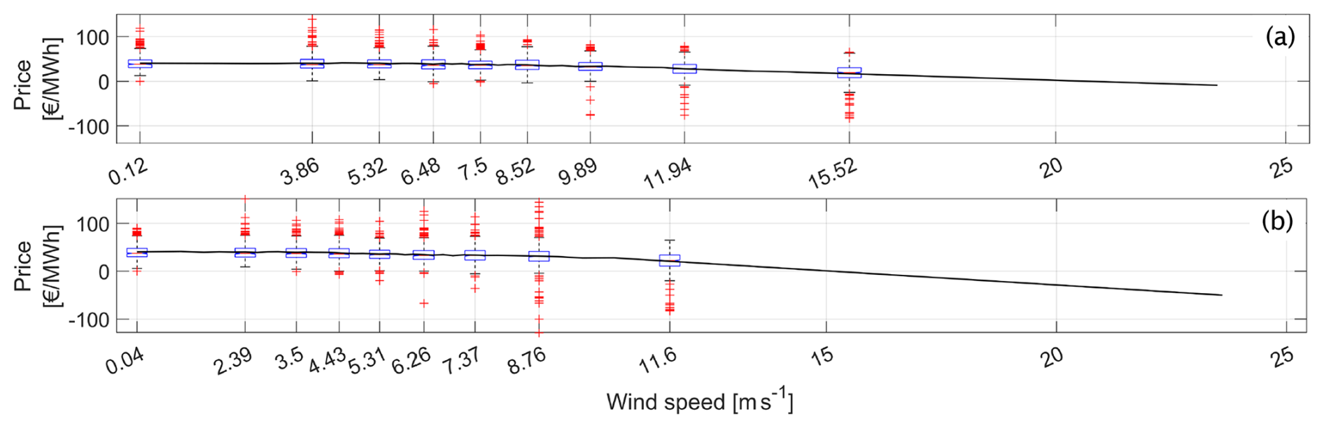
Figure 3 Spot market price (in EUR (MWh)⁻¹) vs. wind speed at 50 m for a site in the north (a) and in the south (b) of Germany. In the boxplots, the central red mark indicates the median, and the bottom and top blue edges of the box indicate the 25th and 75th percentiles, respectively. Whiskers extend to the most extreme data points not considered outliers, whereas outliers are plotted individually using a red “+” symbol. Above 15.52 m s⁻¹, the curve is extrapolated. Adapted from Fig. 8 of Canet et al. (2023).

While the regression model captures the average dependency between market price and inflow wind speed, Fig. 3 indicates a significant spread of instantaneous prices for a given wind speed. This implies that the model represents the expected price conditioned on wind speed but does not capture the full variability in the market signal. As a result, short-term events in which low wind speeds coincide with unusually low (or high) prices are not explicitly resolved. However, the present approach aims at the optimization of the control policy over long-term operating conditions. In this context, the use of an average price signal is acceptable, as it allows for the control strategy to reflect long-term economic effects. Other approaches are being developed to allow wind farms to react to shorter-term electricity price changes, which is particularly relevant for the participation in modern energy markets (Zheng et al., 2026).

3.4.2 Cost model

The second element of the profit equation is the cost model, which estimates the maintenance expenses arising from accumulated damage to the components of each turbine in the wind farm. Maintenance costs are generally divided into two categories: scheduled (preventive) maintenance and unscheduled (corrective) maintenance (DIN Standard 13306:2018, 2018).

Scheduled maintenance involves routine tasks carried out according to a predetermined time plan, often through continuous or periodic monitoring of turbine components. Unscheduled maintenance, on the other hand, is performed after a failure occurs, and the operational readiness of the component needs to be restored. Unscheduled maintenance can also be opportunistic, prompted by condition monitoring to prevent imminent failure.

Walgern et al. (2017) provide a summary of both maintenance categories. Maintenance costs are primarily driven by factors such as equipment repair or replacement costs, the number of technicians required for repairs, failure rates, and operational downtime losses. Scheduled maintenance costs are generally easier to estimate, as they are based on a predefined maintenance plan. In contrast, unscheduled maintenance costs depend on stochastic factors such as mean time between failures, component reliability, and repair time per failure (De Jong, 2007).

This work considers a simplified maintenance cost model, which tries to capture only the fundamental aspects of the complex, variable, and uncertain nature of O&M costs. The formulation is inspired by the discussions in TotalControl (2022a), Bakhshi and Sandborn (2018), Poore (2008), and De Jong (2007). While it is clear that industry certainly has access to more precise cost models, the present one is deemed sufficient as a proof of concept and could be readily replaced with a more accurate one without affecting the general formulation proposed here.

The incurred maintenance costs are written as

$$\begin{array}{}\text{(17)}& \text{Cost}({\mathit{W}}_{\mathrm{a}},\mathit{u})=\sum _{c\in C}{\displaystyle \frac{{\mathbb{C}}_{\mathrm{opex}}^c\left({\mathit{W}}_{\mathrm{a}}\right)}{D_{\mathrm{ref}}^c}}\sum _{i=\mathrm{1}}^N{D}_i^c\left(\mathit{u}\right({\mathit{W}}_{\mathrm{a}}\left)\right),\end{array}$$

where ${\mathbb{C}}_{\mathrm{opex}}^c\left({\mathit{W}}_{\mathrm{a}}\right)$ represents the operation and maintenance costs for component c, while $D_i^c\left(\mathit{u}\right({\mathit{W}}_{\mathrm{a}}\left)\right)$ is the damage in that component for turbine i, which in turn depends on the control actions u triggered on all turbines by the ambient conditions W_a.

The operation and maintenance costs are formulated as

$$\begin{array}{}\text{(18)}& \begin{array}{rl}{\mathbb{C}}_{\mathrm{opex}}^c\left({\mathit{W}}_{\mathrm{a}}\right)& ={\mathbb{C}}_{\mathrm{sch}\text{lost}}^c\left(\right(\mathbb{R}\left({\mathit{W}}_{\mathrm{a}}\right)\text{CF}\sum _{i=\mathrm{1}}^N\left({\mathbb{C}}_{\mathrm{sch}\text{down},i}^c{P}_i^r\right))\\ & +{\mathbb{C}}_{\mathrm{sch}\text{fixed}}^c{P}^r)+{\mathbb{C}}_{\mathrm{unsch}\text{lost}}^c(\left(\mathbb{R}\right({\mathit{W}}_{\mathrm{a}})\\ & \cdot \text{CF}\sum _{i=\mathrm{1}}^N\left({\mathbb{C}}_{\mathrm{unsch}\text{down},i}^c{P}_i^r\right))+{\mathbb{C}}_{\mathrm{unsch}\text{fixed}}^c{P}^r).\end{array}\end{array}$$

The first cost item, depending on coefficients ${\mathbb{C}}_{\mathrm{sch}\cdot }^c$, corresponds to the scheduled maintenance expenses. The second cost item, depending on coefficients ${\mathbb{C}}_{\mathrm{unsch}\cdot }^c$, corresponds to the unscheduled maintenance expenses.

Both scheduled and unscheduled expenses include fixed and variable costs. The fixed costs are assumed to be proportional to the average turbine rating P^r through the coefficients ${\mathbb{C}}_{\mathrm{sch}\text{fixed}}^c$ (for scheduled maintenance) and ${\mathbb{C}}_{\mathrm{unsch}\text{fixed}}^c$ (for unscheduled maintenance). These repair costs account for equipment, labor, and operational personnel expenses.

The variable costs represent the opportunity cost incurred because of production losses during turbine maintenance caused by component c. For scheduled maintenance, these are proportional through coefficient ${\mathbb{C}}_{\mathrm{sch}\text{lost}}^c$ to the revenue lost due to downtime, which is computed as the product of the electricity market price ℝ and the corresponding lost wind farm yield. The latter quantity is calculated as the sum of the products of the rated power outputs $P_i^{\mathrm{r}}$ of each turbine and the turbine component unavailability caused by downtime ${\mathbb{C}}_{\mathrm{sch}\text{down},i}^c$, multiplied by the wind farm capacity factor CF. A similar formula applies to the non-scheduled maintenance, with coefficients ${\mathbb{C}}_{\mathrm{unsch}\text{lost}}^c$ and ${\mathbb{C}}_{\mathrm{unsch}\text{down}}^c$.

O&M expenses are then linearly amortized in Eq. (17) over the reference damage $D_{\mathrm{ref}}^c$ to determine the maintenance cost due to the incurred damage $D_i^c$. The total maintenance cost is obtained by summing the costs for each individual component.

Among other simplifications, the model does not account for the teething and aging effects that typically lead to higher costs at the beginning and end of the lifetime of an asset.

3.4.3 Time discounting

When performing an economic analysis over years-long horizons, it is customary to discount the value of future cash flows, the underlying idea being that the value of one euro in the future is less than the value of one euro today. Following this approach, the net present value (NPV) of economic profit is calculated as

$$\begin{array}{}\text{(19)}& \text{Profit}(\cdot )=\sum _{t=\mathrm{0}}^T{\displaystyle \frac{{\text{Revenue}}_t(\cdot )-{\text{Cost}}_t(\cdot )}{(\mathrm{1}+\mathbb{D}{)}^t}},\end{array}$$

where 𝔻 denotes the discount rate (Short et al., 1995; Shou, 2022).

Time discounting is commonly adopted when evaluating the economic performance of a control policy a posteriori (i.e., after the policy has been synthesized) because it accounts for factors such as inflation, opportunity cost of capital, and economic risk through the computation of the NPV. However, its role during the design of a control policy, such as the one stemming from Eqs. (1a)–(1c) or (4a)–(4c), deserves separate consideration.

In principle, the inclusion of time discounting in the optimal control problem may alter not only the value of the objective function, but also the optimal control policy itself. In fact, since profit generated earlier in the wind farm lifetime has a higher present value than profit generated later on, the optimizer may find it advantageous to exploit the available structural damage budget more aggressively during the early years if this comes with an increased (earlier) economic gain. This might leave a reduced damage budget later on in the lifetime of the assets, which would require a less aggressive control policy and therefore a somewhat reduced energy capture; however, because of discounting, this would have a reduced weight in the overall lifetime cost function. As a consequence of the different weights that actions have over the years when using the NPV as a cost function, the same ambient conditions may no longer correspond to the same control actions at different stages of the wind farm lifetime, leading to an optimal policy that evolves over time.

The proposed formulation naturally accommodates such a behavior. In fact, the economic objective of the reformulated optimization problem expressed by Eq. (4a)–(4c) already accounts for time-dependent quantities through the summation over the epochs y, whereas the structural integrity of the wind farm is enforced by an overall lifetime damage constraint. This way the optimal control policy depends not only on the ambient conditions but also on the epochs. This allows the possible change over time of the control actions, as driven by discounting, while still ensuring that these evolving controls are able to bring the farm to the desired lifetime duration.

We perform a preliminary limited investigation on the effects of time discounting on epoch-dependent control policies later in Sect. 4.1.6. However, to limit the scope of this work, all other test cases studied here assume that each ambient condition is associated with a unique set of turbine control set points throughout the wind farm lifetime. Accordingly, time discounting is not included in the economic model when solving the control synthesis optimization problem expressed by Eq. (4a)–(4c). However, it is accounted for when evaluating a posteriori the economic performance of the resulting control policies.

4 Results and discussion

The economic lifetime-aware formulation is demonstrated in two exemplary scenarios: a first idealized case characterized by a simplified set of environmental conditions causing very frequent waking and a second case featuring a more realistic small wind farm exposed to a wind climate derived from an existing meteorological mast. For both scenarios, the wind farm

• has already operated for half of its target operational life T of 20 years;

• has accrued additional unexpected damage over this duration, which would lead to a premature failure of a component if its operation continued as usual.

The proposed approach is applied to the remaining lifespan of the assets, taking into account the current state of health resulting from accumulated damage. The fatigue constraints target the root of the blades and the base of the tower to avoid their premature failure. These components were chosen because of their critical nature and the significant costs that the wind farm operator would face in the event of failure (Anand et al., 2022; Canet et al., 2021; Stehly et al., 2020). Additionally, in their experimental validation of the lifetime-aware WFC formulation, Braunbehrens et al. (2024) indicate that both the tower base and blade root exhibit distinct responses to varying inflow and control conditions, making them interesting targets also for the present study.

Any component failure leads to maintenance and downtime, as discussed in Sect. 3.4. For simplicity, it is assumed that the fixed costs associated with maintenance, downtime, and the number of maintenance activities remain constant over time, although a more realistic assumption would be to use the classical bathtub behavior. It is further assumed that the ambient wind conditions do not change over time. The set of ambient wind conditions W_a and their probabilities of occurrence are derived from the site wind rose.

Wake control is based on steering, and therefore the decision variables in Eq. (4a)–(4c) are limited to the yaw-offset set points, $\mathit{u}=\left[{\mathit{\gamma }}_{\mathrm{1}},\mathrm{\dots },{\mathit{\gamma }}_i,\mathrm{\dots },{\mathit{\gamma }}_N\right]$, where γ_i is the misalignment of the ith turbine with respect to the incoming wind direction. The bounds on the yaw offsets appearing in Eq. (4c) are ±20° for all the turbines throughout their lifetime.

The load surrogate (see Sect. 3.2 and Appendix A) was trained on the results of 1908 FAST.Farm simulations, conducted for an array of three IEA 3.4 MW reference wind turbines (Bortolotti et al., 2019). The damage limit $D_{\mathrm{ref}}^c$ appearing in Eq. (4b) is chosen as

$$\begin{array}{}\text{(20)}& D_{\mathrm{ref}}^c=\underset{i}{max}\sum _T{D}_{i,\text{greedy}}^c\left({\mathit{W}}_{\mathrm{a}}\right)\forall i\in N,\end{array}$$

which corresponds to the maximum accumulated damage over all the turbines under standard greedy control, where no wake steering is used.

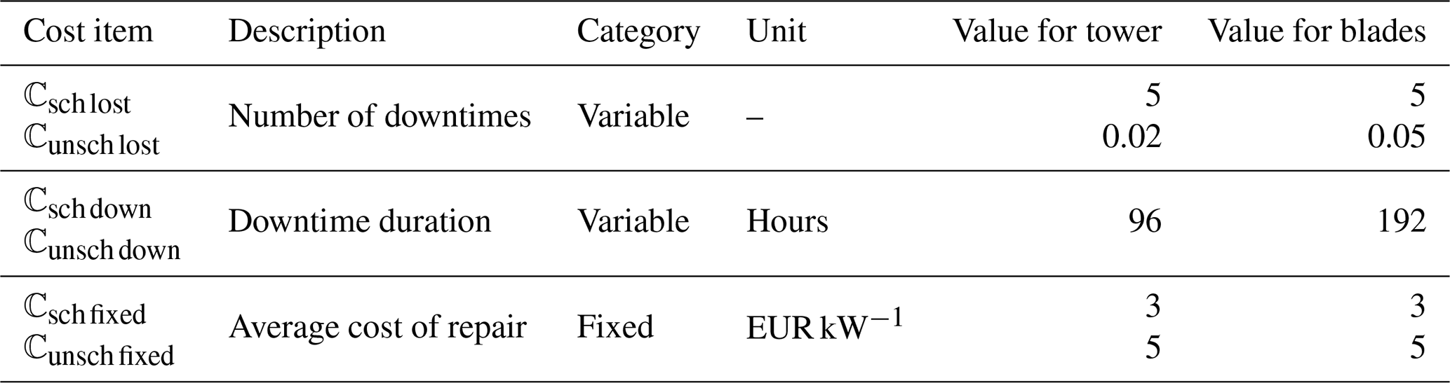
The parameters of the cost model expressed by Eq. (18) are reported in Table 1. The maintenance cost parameters are derived from Poore (2008), Sheng (2013), Pfaffel et al. (2017), Chan and Mo (2017), and Cevasco et al. (2021) and are based on various databases also referenced in Bakhshi and Sandborn (2018).

Table 1 Coefficients of the cost model of Eq. (18).

4.1 Case study I: simple wind farm layout and synthetic wind rose

The first case study evaluates the performance of the proposed WFC formulation in comparison to reference control strategies, including the baseline greedy one, in a simplified case consisting of three turbines and a synthetic wind rose that generates frequent waking. Results are analyzed in terms of yaw offsets, power output, component loading, and lifetime economic performance in terms of revenue, cost, and profit.

One of the main goals of this first example is to quantify the accuracy of the computational framework that supports the synthesis of the control set points. In fact, as discussed in Sect. 3, the framework is based on a fast but low-fidelity engineering flow model (FLORIS), which in general will match with only a limited accuracy the ground truth. In the absence of an even higher-fidelity model of the plant, here the ground truth is assumed to be represented by the mid-fidelity model FAST.Farm. The set points computed by the framework for each WFC formulation are dispatched to the FAST.Farm model, and then various quantities of interest are measured based on its transient response. A quantification of the accuracy of the computational framework is finally obtained by comparing predicted and measured quantities of interest.

4.1.1 Farm layout and wind conditions

We consider three IEA 3.4 MW reference wind turbines (Bortolotti et al., 2019) in an aligned layout with 6 D spacing. This setup is illustrated in Fig. 4b for the baseline greedy case, where all turbines point straight into the incoming wind. The turbine layout resembles a typical WFC demonstrator case for wind tunnel experiments and simulations (Campagnolo et al., 2020). Aligned layouts are also studied in field tests (Göçmen et al., 2022).

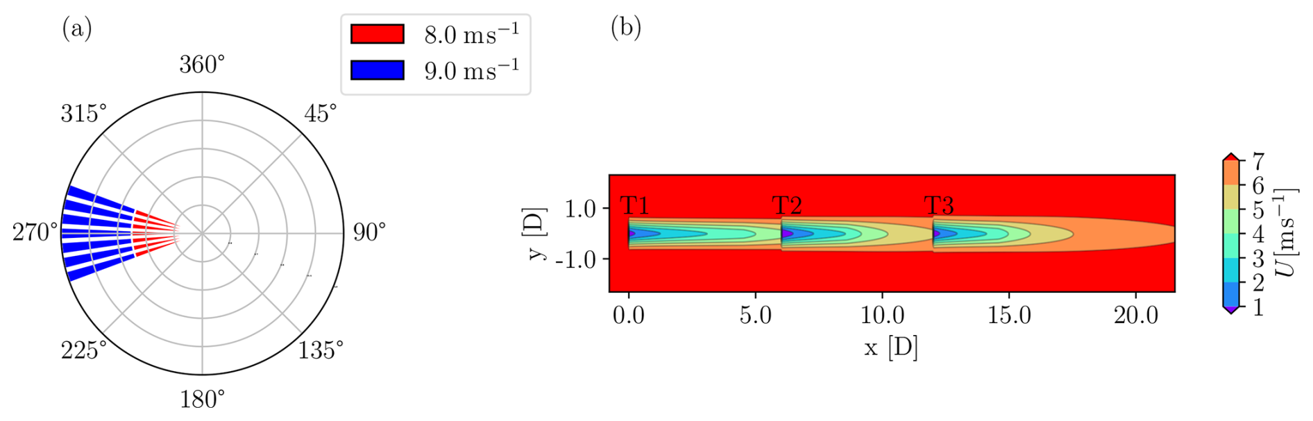
Figure 4 Layout and ambient wind conditions for the simplified case study. Wind rose showing ambient input wind speeds and directions (a). Wind farm layout and wakes at hub height for a wind blowing from the western direction and greedy control (b).

The synthetic wind rose is shown in Fig. 4a. The wind direction spans a sector ranging from 250 to 290°, where the 270° direction is aligned with the turbine layout. Each wind direction sector includes two wind speed bins of 8 and 9 m s⁻¹, each with an equal probability of occurrence. Under these conditions, the baseline greedy formulation results in an overall wake loss of 11 %. The purpose of selecting this wind rose is to evaluate the performance of different WFC strategies without the influence of the frequency distribution of the individual wind condition bins.

For all WFC approaches, T1 and T2 perform wake steering according to their respective control policies, whereas T3 always operates in greedy control mode. Moreover, T2 is assumed to have accumulated 25 % more damage to its components than anticipated in the first 10 years of operation.

4.1.2 Control schedule, power, and load distribution

Figure 5 displays the yaw-offset schedules derived from the different WFC formulations for an ambient wind speed of 8 m s⁻¹ for turbines T1, T2, and T3, respectively from left to right. The x axis reports the ambient wind direction Γ in degrees, while the y axis indicates the optimal yaw offsets in degrees.

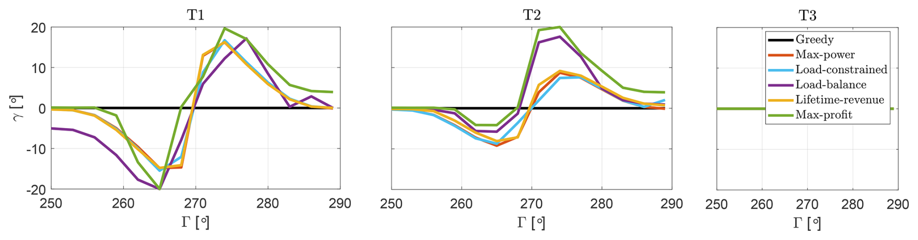
Figure 5 Yaw-offset schedules for T1, T2, and T3 as functions of wind direction Γ, at an ambient wind speed of 8 m s⁻¹, for all the considered WFC strategies. As wake steering is only implemented on T1 and T2, the yaw offset of T3 is constant at 0°.

To evaluate the performance of the various wind farm controllers, transient simulations in turbulent winds are conducted in FAST.Farm, where, for each binned wind condition, the yaw offsets are dispatched to the turbines according to the schedules shown in Fig. 5.

Figures 6, 7, and 8 present the resulting power, blade root DELs, and tower base DELs, respectively. In each figure, the outputs are displayed as panels, with rows corresponding to the six WFC strategies and columns representing the three turbines. The y axis reports the absolute value of the output in the respective units, and the x axis shows the ambient wind direction Γ in degrees. Solid lines represent the outputs measured in the FAST.Farm simulations (labeled “Meas.”), while dashed lines show the corresponding predictions (labeled “Pred.”) obtained during the synthesis of the optimal yaw offsets using the steady-state engineering model FLORIS.

In all panels of Fig. 5, 6, 7, and 8, different colors are used to distinguish the outputs of the six WFC strategies: the baseline greedy strategy is shown in black, the max-power strategy in orange, the load-constrained strategy in blue, the load-balance strategy in violet, the lifetime-revenue strategy in yellow, and the proposed max-profit strategy in green.

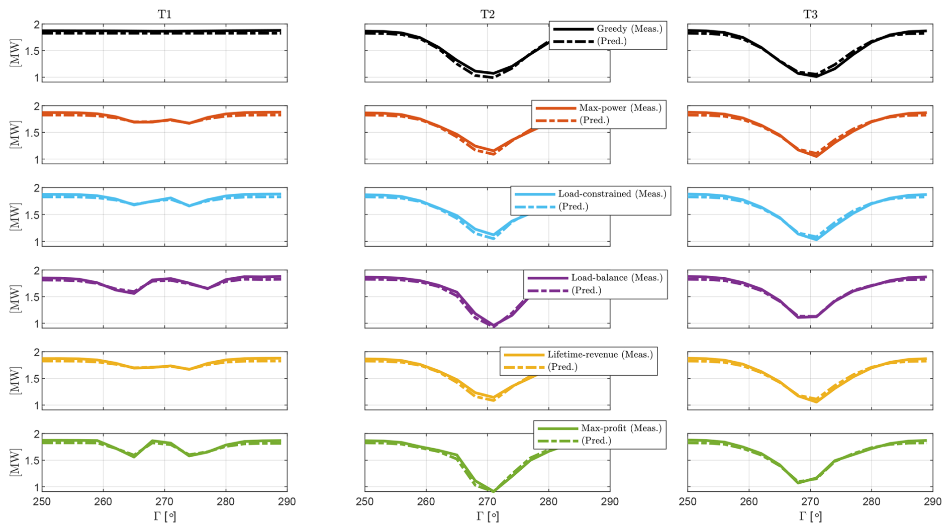
Figure 6 Power output for case study I. The three columns from left to right denote the outputs of the three turbines, T1, T2, and T3, respectively. The six rows from top to bottom denote the six control formulations. In every panel, the x axis indicates the wind direction Γ, and the y axis shows the generated power. Solid curves represent measured values from FAST.Farm, while dashed curves show the corresponding value predicted by the optimization framework based on FLORIS.

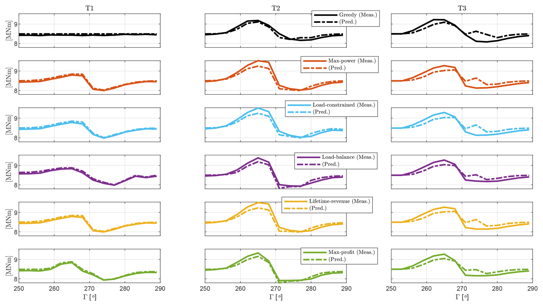
Figure 7 Projected blade root DELs for case study I. The organization of the figure and meaning of the line styles are the same as for Fig. 6.

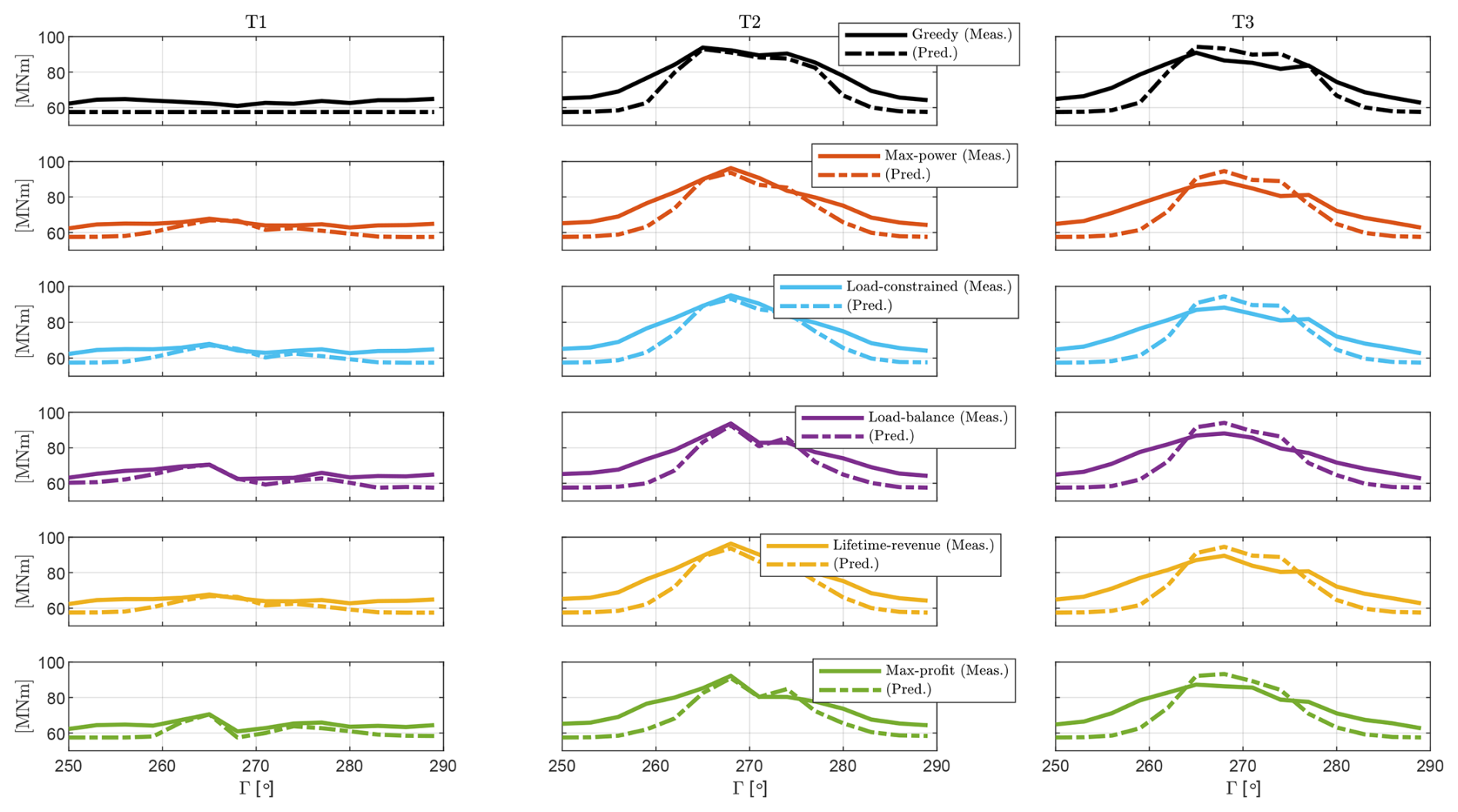
Figure 8 Projected tower base DELs for case study I. The organization of the figure and meaning of the line styles are the same as for Fig. 6.

For all WFC strategies, turbines T2 and T3 operate within the wake of the upstream turbines, resulting in a reduced power output compared to T1, as shown in Fig. 6. In the baseline strategy, the power of the downstream turbines decreases as they enter partial-wake conditions, with the largest power loss occurring under full waking at Γ=270°. Power losses are most significant for T3, as it operates under the combined wakes of both upstream turbines. The power produced by the downstream turbines T2 and T3 is influenced by the available wind speed in the flow, which follows the trend of the RAWS, as shown in Fig. A1a.

The blade root DELs for the baseline formulation show an asymmetric behavior with respect to the ambient wind direction, as seen in Fig. 7. For Γ<270°, the DELs of T2 and T3 are higher than those of T1, while for Γ>270°, the DELs of T2 and T3 are smaller. This asymmetry is primarily driven by the corresponding RAHS, which also exhibits an asymmetric response with respect to Γ (see Fig. A1c).

In contrast, the tower base DELs for the baseline formulation display a symmetric behavior with respect to Γ, as shown in Fig. 8, with both T2 and T3 experiencing higher DELs than T1. This is because tower base DELs are mainly influenced by the RATI, which is higher for the waked turbines (see Fig. A1b) and exhibits a symmetric pattern with respect to Γ.

For an 8 m s⁻¹ ambient wind speed, as shown in Fig. 5, all WFC formulations result in similar yaw offsets for T1. The yaw offsets for T1 are generally higher in magnitude than those for T2, as T1 operates in clean inflow conditions, which are typically associated with a smaller total loading compared to the waked inflow conditions experienced by T2. Consequently, T1 has a larger available budget to accommodate additional load increases due to active wake steering, resulting in larger yaw offsets compared to T2.

For T1, the highest yaw offset for the four damage-aware formulations – load-constrained, load-balance, lifetime-revenue, and max-profit – is reached farther away from the aligned condition, compared to the max-power strategy. The situation is different for T2, where the damage-aware strategies exhibit a more aggressive wake steering for Γ>270° and a less aggressive steering behavior for Γ<270° compared to the max-power strategy. This is because the yaw schedules are primarily influenced by blade loads, which exhibit an asymmetric behavior with respect to Γ. As a result, it is beneficial to employ more aggressive wake steering for Γ>270° as it reduces blade root DELs, while for Γ<270° wake steering increases these same loads.

Compared to the baseline greedy case, all WFC strategies result in a slight decrease in power for T1 and an increase in power for T2 and T3, as shown in Fig. 6. Consequently, all WFC strategies lead to an overall power gain for the wind farm. Additionally, a comparison between the solid and dashed lines for all strategies reveals that the measured turbine power outputs closely align with the estimated values. This high level of accuracy is due to the precise estimation of RAWS by the engineering flow model used by the optimization framework (refer to Sect. 3.1 for details). Since RAWS is the primary driver of power production, the predicted power closely matches the measured one for the yawed turbine T1, the waked turbine T3, and the yawed and waked turbine T2.

Active wake control leads to an increase in blade root DELs for all turbines when Γ<270° and a slight decrease in DELs for Γ>270°, as shown in Fig. 7. The variation in blade root DELs is most significant for T2, as it experiences the combined effects of operating in a waked inflow and performing wake steering. Additionally, a comparison of the solid and dashed lines indicates that the blade root DELs are well predicted by the optimization framework (cf. Appendix A), which effectively captures the trends in load variation with respect to Γ for T1 (yawed), T3 (waked), and T2 (yawed and waked). This accuracy is especially important for load-aware strategies, where optimal yaw offsets are directly influenced by these variations in loading.

For the tower base, as shown in Fig. 8, active wake control leads to a slight increase in DELs for the yawed turbine, while it significantly reduces DELs for the downstream turbines. Since tower base DELs are primarily driven by RATI, deflections of the upstream wake result in lower RATIs for the downstream turbines, leading to reduced loading. Additionally, a comparison of the solid and dashed lines reveals that, for all control strategies, tower loads are consistently underpredicted in partial-wake conditions (Γ<265° and Γ>275°) and overpredicted in full-wake conditions ($\mathrm{265}\mathit{°}\le \mathrm{\Gamma }\le \mathrm{275}$°). However, the optimization framework still captures the trends in tower load variation with good accuracy. The observed mismatch is primarily attributed to the presence of rotor uptilt in FAST.Farm, which leads to vertical wake displacement and vertical shear at the rotor inflow. In FLORIS, however, the presence of a wake velocity deficit does not change the vertical shear. In addition, FLORIS does not account for vertical wake displacement due to rotor tilt. Therefore, predictions generated by the optimization framework slightly differ from those obtained from FAST.Farm. Despite this, the under- and overpredictions generally cancel each other out for the inflow conditions considered in this case study. The impact of this small net prediction mismatch on lifetime performance is discussed in the following section.

4.1.3 Lifetime consumption

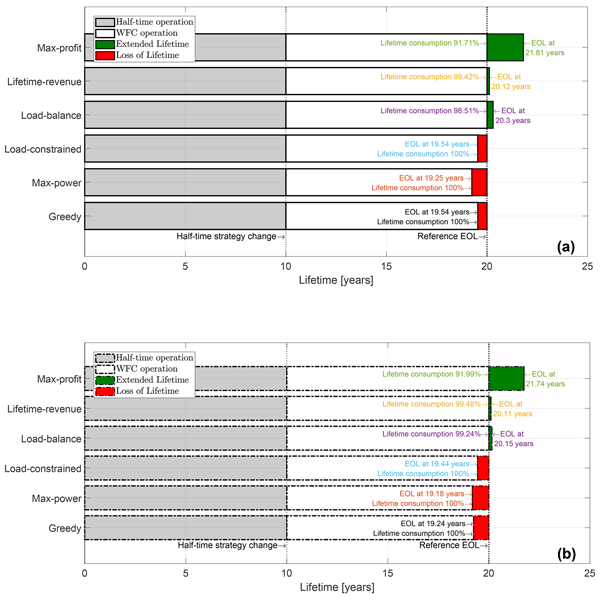
Figure 9 illustrates the lifetime consumption of the wind farm for all considered WFC strategies. Lifetime consumption is determined by the accumulated fatigue damage on the components. For simplicity, we assume that the wind farm reaches its end of life (EOL) when any component of any turbine reaches its EOL. While this is clearly an approximation, it is used here to avoid complicating the analysis further with various possible scenarios. A component reaches its EOL when the ratio of the accumulated damage $D_i^c\left(T\right)$ (cf. Sect. 3.3) and the reference damage $D_{\mathrm{ref}}^c$ equals 1 (cf. Eq. 4b), which corresponds to a lifetime consumption of 100 %.

Figure 9a reports the lifetime consumption that results from dispatching the optimal yaw offsets to the turbines in the transient FAST.Farm simulations, while Fig. 9b shows the predictions by the optimization framework. In both figures, lifetime consumption is represented as horizontal bars, with each bar corresponding to a specific WFC strategy. The x axis represents time in years, and the y axis lists the six WFC strategies.

The performance of the wind farm is assessed over a 20-year operational life, which is the goal desired EOL. The WFC strategies are implemented after the wind farm has operated under the baseline greedy strategy for 10 years (half-time strategy change). Consequently, each bar is divided into shaded regions representing four distinct phases:

• The gray region indicates the lifetime consumed while operating with the baseline greedy strategy.

• The white region represents the lifetime consumed while operating with the different WFC strategies.

• The red region denotes the lost lifetime when the EOL (i.e., when the accrued damage is equal to the allowed damage limit) is reached before the goal EOL.

• The green region represents the gained or extended lifetime, when the accrued damage at the goal EOL is below the allowed damage limit. The remaining useful life is linearly extrapolated to estimate the additional operational years.

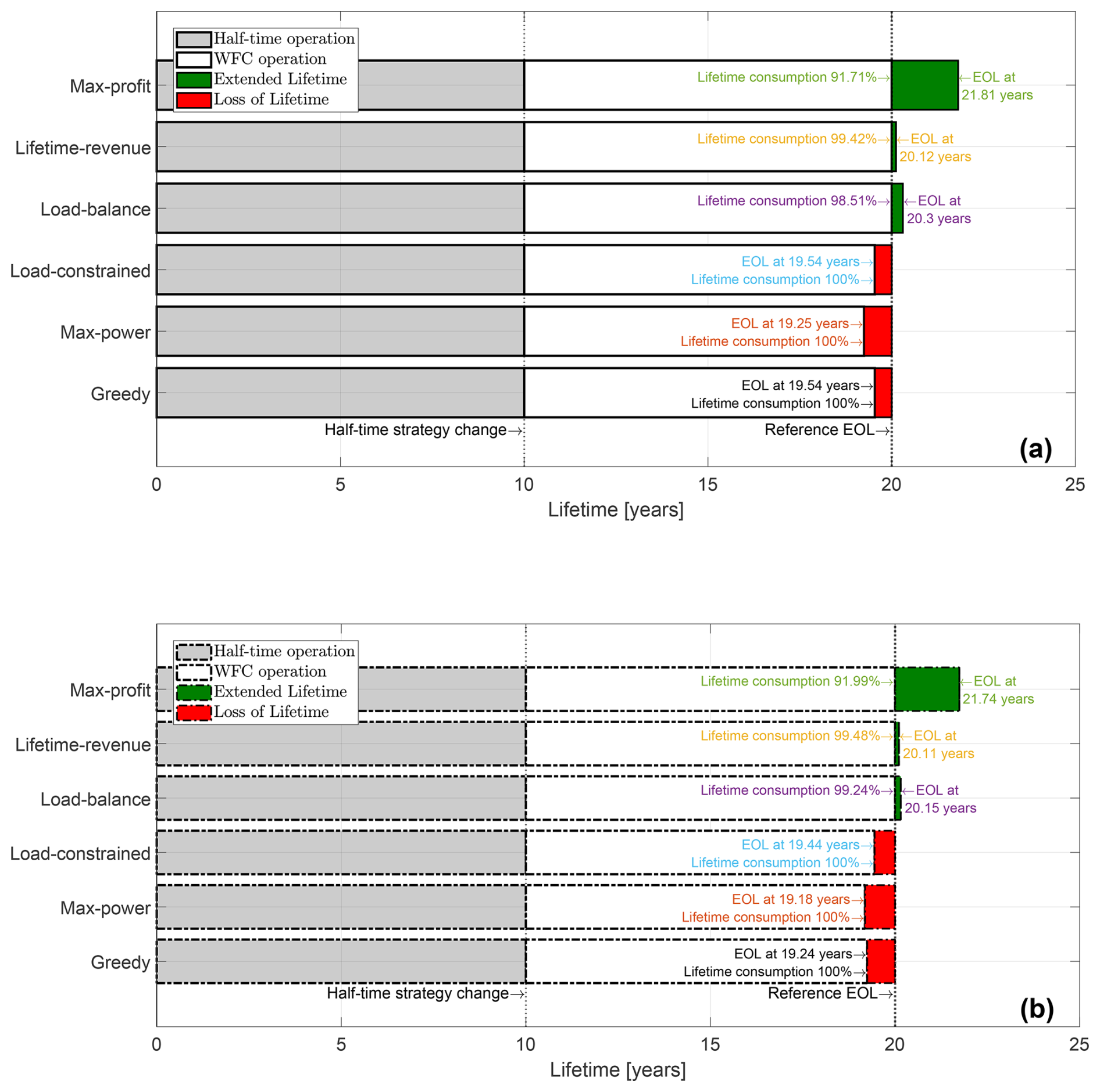
Figure 9 Lifetime consumption of the wind farm for all WFC strategies for case study I. The solid outline of the horizontal bars in panel (a) denotes values measured on FAST.Farm simulations, whereas the dashed outline in panel (b) shows the corresponding predicted values from the optimization framework.

A close examination of Fig. 9a reveals that, when operating under the greedy, max-power, and load-constrained strategies, the wind farm fails to reach the goal EOL, resulting in a loss of operational years. This clearly undesirable effect results from the elevated initial damage assumption introduced in Sect. 4.1.1, where one turbine is assumed to have accumulated more damage during the first 10 years of operation than anticipated at the design stage. Since the greedy, max-power, and load-constrained strategies prioritize short-term power production and do not account for long-term damage balancing across the fleet, the already over-utilized turbine continues to experience relatively high loading. This accelerates damage accumulation and causes the turbine to reach its damage limit before the nominal design lifetime. In contrast, the remaining strategies – load-balance, lifetime-revenue, and max-profit – operate in a more damage-aware manner, leading to a gain in operational years beyond the goal EOL.

The max-power strategy yields the shortest operational life. This suggests that the symmetric wake steering that it employed for T2 (cf. Fig. 5) may enhance energy production but also accelerates fatigue accumulation. As a result of its own activity, T2 experiences a significant increase in blade root DELs in the sector Γ<270° (cf. Fig. 7), which is not offset by the modest decrease due to the wake steering of T1, as discussed in Sect. 4.1.2. Consequently, this wind turbine suffers a higher fatigue damage, leading to a reduction in operational life.

The load-constrained strategy results in a less aggressive yaw-offset schedule compared to the max-power strategy because of the load constraints enforced by Eq. (6b), which account for the loading in individual wind condition bins. However, notwithstanding the presence of these load constraints, this strategy still fails to reach the desired lifetime duration. This is because, as discussed in Sect. 1, the fatigue budget for a specific bin of ambient conditions depends not only on the fatigue damage accumulated within that bin, but also on the damage accumulation from the other bins the wind farm is exposed to. In other words, from a wind farm lifetime perspective, the control actions for a given wind input condition in load-aware operation are influenced by the relative impact of this condition in relation to others. Since the load-constrained formulation only considers individual bins, it overlooks the cumulative effects of other bins, which ultimately results in a loss of lifetime.

The situation is different for the load-balance strategy, which not only reaches but actually extends the intended EOL. However, because the optimization problem used for synthesizing its control set points does not explicitly impose constraints to guarantee a desired lifetime (see Eq. 7a–7b), the performance that is observed here cannot be expected in general. For other farm layouts and inflow conditions, this formulation may not ensure that the wind farm will operate over a specific lifetime, despite the tuning of the weights of the two terms of the cost function.

As anticipated, the lifetime-revenue strategy ensures that the wind farm reaches the desired operational life. This is because the strategy accounts for the combined loading from all wind conditions the farm experiences throughout its lifetime while simultaneously optimizing farm power and, consequently, revenue.

The proposed max-profit formulation, in addition to explicitly considering lifetime constraints, finds the most profitable way of operating the assets throughout their lifetime. It does so by not only focusing on the power output of the individual turbines, but also considering the total energy yield and balancing it against the O&M costs resulting from accumulated damage. Compared to the lifetime-revenue formulation, the max-profit strategy adopts a more aggressive wake steering in partial-wake-overlap conditions ($\mathrm{260}\mathit{°}<\mathrm{\Gamma }<\mathrm{280}$°) for T1 and implements one-sided wake steering for Γ>270° to reduce blade root DELs while avoiding wake steering altogether for Γ<270°. This results in an optimal balance between accumulated damage and revenue, enabling the wind farm to operate for the desired duration while maximizing economic profit throughout its operational life.

Figure 9b shows the estimated lifetime consumption based on the predicted blade root DELs (dashed curves in Fig. 7) and tower base DELs (dashed curves in Fig. 8) for all WFC strategies. By comparing the predicted quantities of Fig. 9b with the measured ones of Fig. 9a, it appears that the optimization framework is capable of estimating lifetime consumption with reasonable accuracy, with only slight underpredictions. The minor mismatches shown in Figs. 7 and 8 have only a minimal impact on the overall lifetime consumption and remaining useful life.

4.1.4 Lifetime economic performance

Figure 10 illustrates the economic performance of the wind farm over its lifetime. Figure 10a shows the economic profit calculated on the FAST.Farm simulations, while Fig. 10b displays the expected economic profit predicted by the optimization framework using the engineering model FLORIS. In both figures, the vertical bars represent the time-discounted economic profit, i.e., the difference between the economic revenue from wind farm yield and the sum of economic costs from O&M and lost lifetime. The economic profit is expressed in relative terms with respect to the greedy baseline over the 20-year operational duration. The height of the bars (i.e., the relative profit) is also reported in white on each bar to ease comparison.

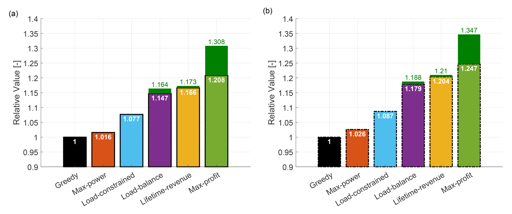
Figure 10 Time-discounted lifetime profit for all WFC strategies for case study I. The solid outline of the vertical bars in panel (a) denotes measured values based on FAST.Farm, while the dashed outline in panel (b) denotes the corresponding values predicted by the optimization framework. The shaded green extensions denote the additional economic gain generated when the farm operates beyond the goal EOL and until its lifetime is finally exhausted.

As discussed in Sect. 3.4.3, while the control actions were computed without considering time discounting, the economic performance is quantified taking time discounting into account. The present value of future profits is actualized using an annual discount rate of 8 %, which is a typical value for wind energy projects (Stehly et al., 2024).

Additionally, in Fig. 10 some strategies include stacked green bars, which represent the extra economic gain due to lifetime extension. For these strategies, the numbers written in green above the bars denote the additional relative profit that is gained if the wind farm continues to operate beyond its goal EOL and until its lifetime is finally exhausted.

Figure 10a shows that all WFC strategies result in higher economic profit compared to the baseline greedy formulation. Profits are notably higher for the damage-aware strategies. This indicates that incorporating damage into the design of wind farm controllers – whether accurately or through approximations – has a significant impact on economic profit.

Both the max-power and load-constrained strategies experience a loss of lifetime, which in turn leads to a loss of revenue. The max-power strategy suffers a larger loss due to its shorter operational life. The load-constrained strategy, on the other hand, incurs smaller costs due to a slightly lower damage accumulation. As a result, the max-power strategy only achieves a 1.7 % increase in profit, while the load-constrained strategy sees a larger increase of 7.7 %.

The load-balance strategy, thanks to a careful tuning of the weights in its optimization objective, results in an additional 7 % profit over the load-constrained strategy. The lifetime-revenue strategy further optimizes loading by simultaneously considering all various operating conditions, which leads to a profit increase of 16.5 % over the baseline.

Finally, the proposed max-profit formulation ensures the desired lifetime is met while maximizing profit. Although it generates less revenue than the lifetime-revenue strategy, it saves significantly on maintenance expenses due to a reduced accumulated damage. This results in an additional 4 % profit compared to the lifetime-revenue strategy.

The importance of optimizing profit, rather than solely focusing on revenue, is further stressed by the additional earnings that can be gained from the extended operational life of the wind farm. The max-profit formulation achieves a 30 % profit gain over the baseline and an additional 13 % gain compared to the lifetime-revenue strategy.

Similarly to lifetime consumption, even lifetime profit is quite accurately predicted by the optimization framework, as shown in Fig. 10b. The dashed outline of the vertical bars in Fig. 10b represents estimated values, while the solid outline of the bars in Fig. 10a corresponds to measured values. When comparing the two figures, it appears that there is a slight overprediction of lifetime profit for all WFC strategies compared to the respective baseline. This effect can be attributed to the previously observed overprediction of component loads.

4.1.5 Sensitivity to changes in the economic model parameters

The economic lifetime-aware WFC optimization problem is affected by significant aleatoric and epistemic uncertainties. While the underlying models in the optimization framework use deterministic inputs and outputs, because of these uncertainties the response that the computed control actions generate in the wind farm and their performance indicators are expected to change to some unknown degree. Clearly all aspects of the formulation are affected by uncertainties. However, the flow and load models – together with their uncertainties – used here are also widely employed in the literature to treat similar problems. The situation is different for the economic model. For example, spot market prices can vary in a very significant manner in time and space. Additionally, the cost model adopted here is highly simplified and might not fully reflect the complexities of the economics of wind farm O&M. The effects of loads on cost are especially a problem that is not sufficiently documented in the open literature. Because of these reasons, here we try to quantify the effects that changes in the parameters of the cost model might have on the results. While this analysis is far from being a comprehensive quantification of all uncertainties, it is hoped that it contributes to shedding some light on the robustness of the conclusions so far with respect to the economic modeling aspects of the problem.

Figure 11a illustrates the variations in lifetime profit resulting from changes in the parameters of the economic model (cf. Sect. 3.4). The y axis shows the relative lifetime profit compared to the baseline greedy case, while the x axis denotes the different WFC strategies. For each vertical bar, the numbers from top to bottom represent the upper, average, and lower profit values, respectively.

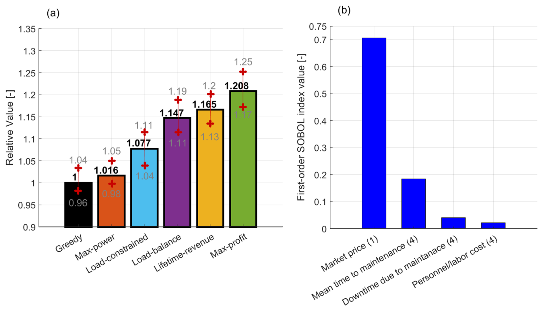
Figure 11 Quantification of the uncertainties in lifetime economic performance caused by uncertainties in the economic model parameters of Sect. 3.4. Results of a Monte Carlo analysis for a uniformly distributed economic parameter space, where the black numbers denote the mean value and the gray numbers the corresponding uncertainty bounds (a). Results of a variance-based parametric sensitivity analysis for the max-profit strategy, where the vertical bars represent SOBOL indices for different cost items (b).

Uncertainties are calculated by varying the economic model parameters, assuming uniform distributions for each. On the revenue side, the varied parameter is the electricity market price ℝ_avg. On the cost side, for each component the varied parameters include all six maintenance factors appearing in Eq. (18). Since we consider both the blade and tower components, a total of 13 parameters are varied in the uncertainty analysis. For all parameters, we consider a variation of 8 % around its nominal value listed in Table 1.

The uncertainty quantification is performed using Monte Carlo analysis, where the parameter space is randomly sampled until the mean and the 25th and 75th percentiles of profit converge.

The results in Fig. 11a show that, for all WFC strategies, a maximum variation of 8 % in the parameters leads to uncertainties varying only between 3 % and 4 %. This indicates that, for all control strategies, the lifetime profit is affected only to a modest degree by uncertainties in the economic parameters. The same analysis was repeated for variations between 4 % and 12 % in increments of 2 %, observing a nearly linear behavior of the upper and lower bounds of profit.

To better understand the sources of uncertainty in lifetime profit, a variance-based sensitivity analysis is conducted for the max-profit strategy by varying the 13 parameters of the economic model. The results of the analysis are presented in terms of first-order sensitivity coefficients, also known as first-order SOBOL indices (Saltelli et al., 2010). The sensitivity coefficient $S_{X_k}$ indicates how much the output variance Var(Y) can be reduced, on average, if the uncertainty associated with the input variable X_k is fully known, where the output is some known function f(⋅) of the inputs, i.e., $Y=f(X_{\mathrm{1}},X_{\mathrm{2}},\mathrm{\dots },X_k,\mathrm{\dots })$.

The resulting SOBOL indices are grouped into four qualitative categories and are reported in Fig. 11b. The number of parameters in each category is indicated in parentheses. Results indicate that the uncertainty in electricity market prices is the most significant contributor to the overall uncertainty. This is because market prices directly affect both the accrued revenue and the lost revenue due to downtime. The second-largest source of uncertainty is the mean time to failure, which directly impacts the frequency of maintenance activities and the associated costs. While the remaining two categories contribute relatively less, their absolute impact is still noteworthy. This further emphasizes the importance of quantifying the uncertainties associated with failure rates and other O&M parameters.

4.1.6 Preliminary assessment of the impact of time discounting

This section presents a preliminary investigation of the possible effects of time discounting (see Sect. 3.4.3) by considering multiple epochs within the optimal control synthesis based on Eq. (4a)–(4c). Specifically, we would like to verify whether time-evolving control actions emerge or not as a result of the different weights given over time by an NPV-based cost function. To try to give a first answer to this interesting question, the remaining 10-year asset lifetime is divided into two 5-year epochs. The NPV is calculated using a discount rate of 8 %, and we consider the farm layout and wind conditions described in Sect. 4.1.1. However, T2 is assumed to have accumulated 40 % more damage to its components than anticipated in the first 10 years of operation.

Two time-discounted formulations are considered. The first, referred to as max-profit NPV, accounts for the lifetime constraint within the WFC optimization of Eq. (4a)–(4c). The second, named max-profit NPV no-constraint, is a simplified variant that does not account for the lifetime constraint. This latter formulation is introduced to examine whether the optimal control strategy changes across epochs solely as a result of time discounting, when no lifetime budget limits are imposed. Both formulations are compared with the greedy and max-profit formulations, which consider a single epoch.

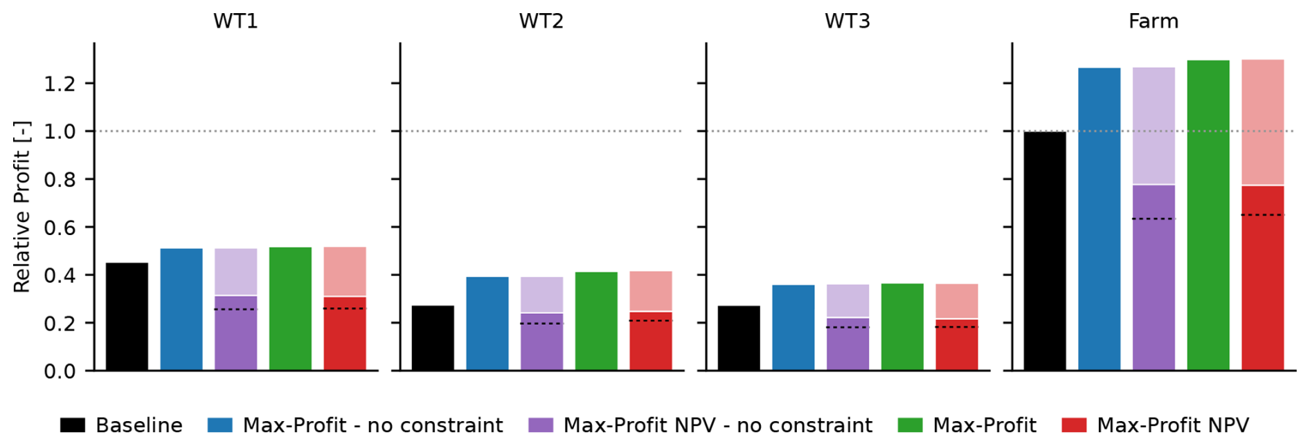
Figure 12 Time-discounted lifetime profit for various max-profit formulations for case study I, considering an 8 % discount factor over different epochs. The profit values for the different formulations are normalized with respect to the lifetime profit of the greedy baseline case.

Figure 12 presents the lifetime profit for the different WFC formulations, expressed as present values and normalized by the corresponding greedy values. The figure compares greedy (black), single-epoch max-profit with (green) and without (blue) lifetime constraints, and two-epoch max-profit NPV with (red) and without (purple) lifetime constraints. For greedy and single-epoch max-profit, discounting is not included in the optimization, and it is applied only a posteriori when calculating the present values for comparison. For the two-epoch max-profit NPV formulations, discounting is directly included in the optimization cost function, and the optimization outputs are shown. The two-epoch results are presented as stacked bars, with lighter and darker shades denoting the first and second epochs, respectively. A horizontal black line marks 50 % of the total bar height, while a white line separates the two epochs.

The max-profit NPV no-constraint formulation produces essentially the same results as its corresponding non-NPV max-profit no-constraint formulation, with no appreciable difference between the control strategies in the two epochs. This is because, in the absence of lifetime constraints, discounting only changes the relative weight of the objective across epochs and introduces no additional constraint or trade-off to drive different control actions.

However, a similar result is also observed for the finite-lifetime-budget case when comparing max-profit NPV with its corresponding non-NPV max-profit formulation. The lifetime profit remains very similar with and without discounting. Moreover, the difference in the heights of the two NPV epoch contributions results solely from discounting; in fact, when discounting is removed from post-processing, the lifetime economic metrics of the two epochs are almost identical (this is not shown in the figure for simplicity of graphic representation).

This limited effect in the finite-lifetime-budget case is attributed to the fact that – in this particular case – there is not a more aggressive control policy that produces more power at the cost of higher damage (which is the primary mechanism that would drive time-evolving control policies, as argued in Sect. 4.1.6). In fact, Figs. 6, 7, and 8 show that wake steering not only increases power, but also decreases loading for the more damaged turbine T2 when compared to the greedy policy. Therefore, there is not any incentive to abandon wake steering in the later epoch. This is probably also due to the limited freedom left to the optimizer, which can only use steering but not induction control. If the turbines could be derated – a control mode where turbines are operated below their available aerodynamic power, which was not considered in this work for simplicity – they could drastically reduce loading at the expense of a decreased capture. In such a situation, one could expect the control policy to prioritize wake steering in the earlier epochs (because it gives a higher early profit due to its improved capture, which is highly rewarded because of discounting) and move away from it later in life (because steering has created more damage, and a derated operation that induces less loading allows the lifetime constraint to be satisfied, the reduced profit playing a limited role, here again because of discounting).

Overall, these results show that the proposed multi-epoch formulation can indeed account for time discounting and – in principle – permits the control strategy to evolve over the asset lifetime. However, for the present highly simplified test case, this flexibility produces only negligible changes in the control actions. The complexity of the general NPV-based problem – which may depend on many factors such as layout, inflow conditions, control set points, accumulated damage, lifetime constraints, etc. – clearly deserves more extensive dedicated studies, which could not fit in the scope of the present work.

4.2 Case study II: realistic wind farm layout and wind rose

The goal of the second case study is to apply the proposed WFC approach to a more complex and realistic scenario. In this case, the wind farm is a small offshore cluster operating under field-measured wind conditions. The primary objective is to evaluate how the new method performs for a larger cluster of turbines, focusing on how the increased turbine count and varied inflow conditions affect the solution. Additionally, this case study aims to assess the growth of the computational cost of the proposed method as the wind farm cluster size increases.

For comparison, all reference control formulations presented in Sect. 2.7 are also considered here. The results shown in the following are those obtained by the optimization framework. Since the previous section showed that the framework – notwithstanding its underlying low-fidelity flow model – provides accurate predictions of lifetime quantities, additional validation using FAST.Farm was deemed not to be necessary in this case.

4.2.1 Farm layout and ambient wind conditions

This case considers the nine-turbine wind farm layout defined in the CL-Windcon project (Irigoyen, 2017). The turbines are arranged in a regular grid, with a spacing of 7 D in the x direction and 5 D in the y direction, as shown in Fig. 13b. The wind conditions are based on reanalysis data obtained from the site of the Hollandse Kust Nord offshore wind farm (Hersbach et al., 2020), which is also being considered in the SUDOCO project (Gebraad et al., 2024). The corresponding wind rose is shown in Fig. 13a. The wind speed range is limited to between 6 and 10 m s⁻¹. It is assumed that these ambient conditions remain constant over the various years of operation.

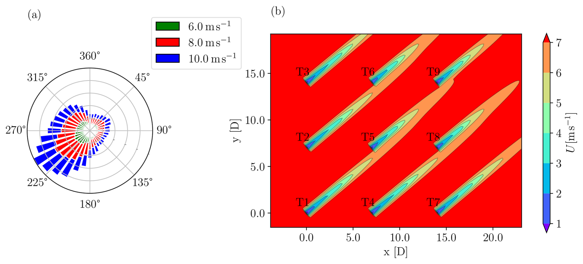
Figure 13 Layout and wind rose for the realistic case study. Wind rose (a). Wind farm layout and wakes at hub height for wind blowing from the southwestern direction (b).

Since the wind inflow comes from all directions, all turbines operate in a combination of waked and free-stream conditions. The AEP loss due to wake interaction in greedy mode, as calculated by FLORIS, is approximately 5 %. Similarly to case study I, the market price is assumed to vary around an annual average, depending on the ambient wind speed. An annual discount rate of 8 % is used to estimate the present value of future profit (Stehly et al., 2024), as discussed in Sect. 3.4.3. For simplicity, the number of maintenance activities, fixed maintenance costs, and maintenance downtime per component are assumed to remain constant over time. Here again, loads, DELs, and damage are computed at the tower base and blade root.

This case study assumes a 20-year lifetime. During the first 10 years, the farm operates in greedy control mode before switching to one of the WFC formulations for the second half of its lifetime. As in case study I, one turbine (T5) is assumed to have accumulated more fatigue damage than the others. T5 operates in waked conditions most of the time and with its wake also affects the turbines at the trailing edge of the farm. As a result, it is assumed that after 10 years turbine T5 will have accumulated 75 % more damage than expected. This additional damage is larger than in case study I, as the more realistic wind conditions in this study are less challenging than the single wind sector considered in that case. This is clearly an idealized exemplary situation. In another scenario, T5 might represent a machine that suffers from higher failure rates than the others, for example because of manufacturing issues, extra vibrations suffered during its erection phase, or other possible reasons.

4.2.2 Lifetime consumption

Figure 14 shows the lifetime consumption for the wind farm for all WFC strategies. Similarly to Fig. 9, the horizontal bars represent the operational years of the wind farm, with a goal EOL of 20 years. As previously noted, the various WFC strategies are deployed after the first 10 years of operation.

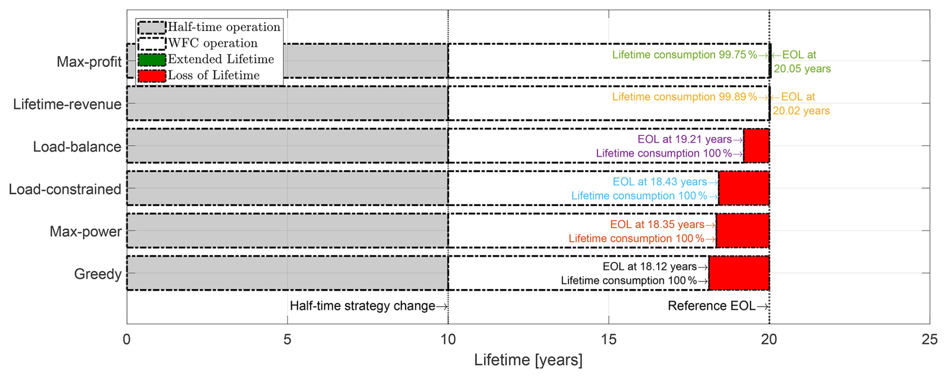
Figure 14 Lifetime consumption of the wind farm for case study II for all considered WFC strategies.

The figure adopts the same layout as used in Sect. 4.1.3. The shaded green region indicates an achieved extended lifetime beyond the desired goal EOL, while the shaded red region represents lost operational time due to having exhausted the lifetime before the desired EOL.

Figure 15 shows that all WFC strategies result in longer operational times than the baseline greedy mode. Strategies that account for component damage – either explicitly or indirectly – perform better from this point of view than the max-power strategy, which does not account for loads in its formulation. However, only the lifetime-aware strategies, specifically lifetime-revenue and max-profit, ensure operation throughout the entire goal EOL. This is because the optimal yaw offsets for these two strategies are less aggressive, as the controllers consider the inflow and operational conditions at all turbines over their entire lifetime. Furthermore, the proposed max-profit formulation provides a slight lifetime extension, allowing the wind farm to operate beyond the goal EOL, thus generating additional revenue.

4.2.3 Lifetime economic performance

Figure 15 reports the time-discounted lifetime economic performance of the wind farm. Results are displayed in the same format used for Fig. 10b. The vertical bars show the profit relative to the baseline profit obtained in greedy mode over the 20-year operational duration. The white numbers represent the heights of the bars (i.e., the relative profit) to ease comparison among the various WFC strategies.

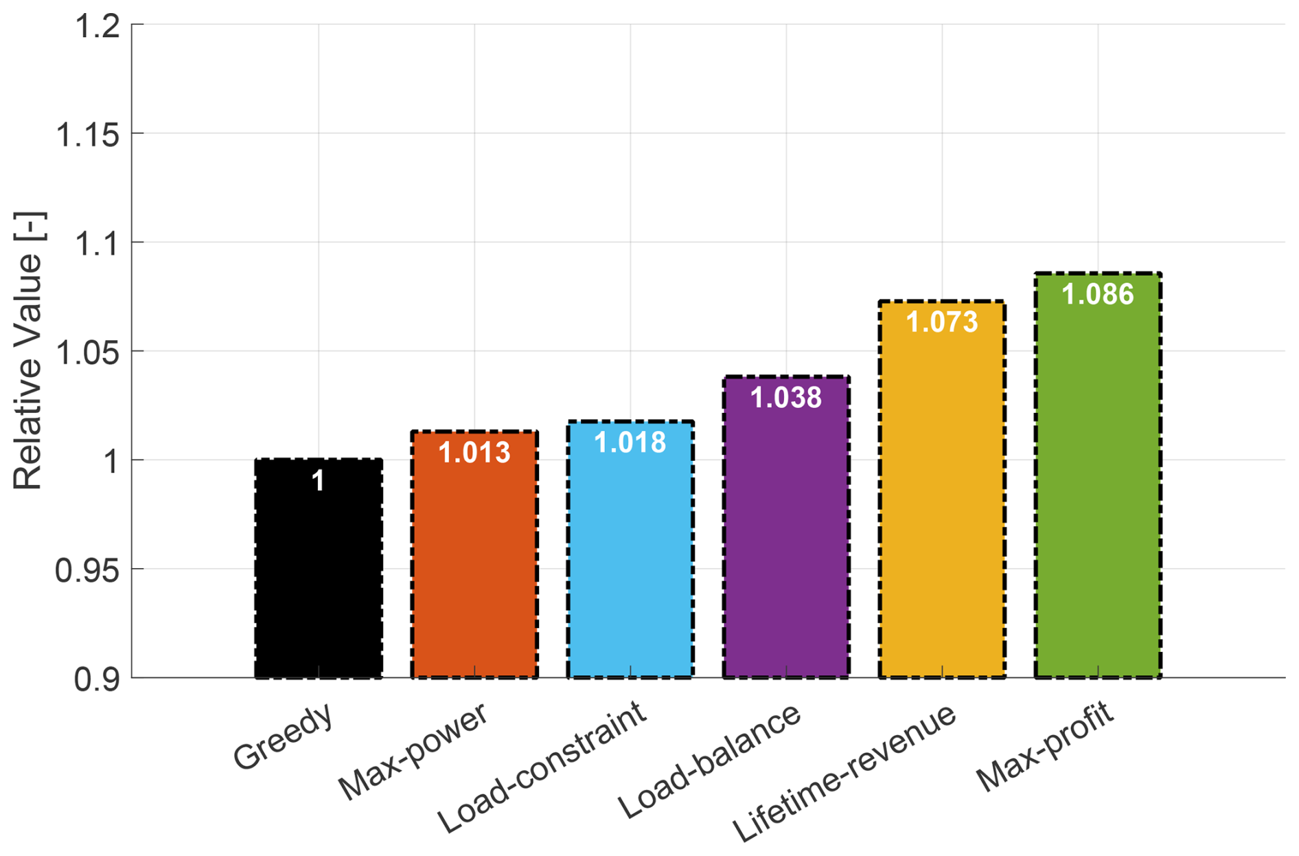
Figure 15 Time-discounted lifetime profit of the wind farm for case study II for all WFC strategies.

All strategies result in economic gains with respect to the baseline greedy scenario. However, due to loss of lifetime, the max-power, load-constrained, and load-balance strategies show relatively minor gains, which depend on their specific revenue losses. In contrast, the two lifetime-aware strategies – lifetime-revenue and max-profit – yield significantly higher gains of 7.3 % and 8.6 %, respectively, thanks to their guaranteed operation over the full desired lifetime.

Of these two, the best performer is the max-profit formulation because of its ability to include the effects of loads on cost and hence on profit.

4.3 Computational effort

The proposed approach requires a set point optimization for all turbines in all possible ambient wind conditions throughout their entire lifetime. The resulting one-shot optimization can become computationally demanding. To assess the growth of the computational cost, farms of varying number of turbines are investigated. Starting from the 3×3 layout, the configuration is first reduced to a 2×2 setup and then extended to 4×4 and 5×5 configurations, all while maintaining the same x–y separation distances. The other problem parameters (wind rose, goal EOL, time of deployment of WFC, etc.) are unchanged with respect to the 3×3 case.

The optimization problem is solved iteratively until numerical convergence is achieved. All optimizations are performed on a desktop computer with an Intel^® Core™ i7 processor, 8 GB of RAM, and a 64 bit operating system.

Figure 16 presents the results of the computational performance test in a log–log plot. The x axis represents the total number of turbines in the farm, while the y axis shows the wall clock time taken by the optimization problem to converge. Time is normalized with respect to the 2×2 configuration, which required 0.24 h to complete. This wall clock time is a value with little practical meaning, as hardware performance evolves quickly, and no effort was made to optimize the code for speed. Therefore, the more useful piece of information provided by the figure is the slope of the computational cost growth.

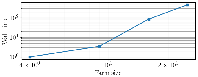
Figure 16 Increase in wall-clock time with the number of turbines in a regular grid with spacings of 7 D and 5 D in the x and y directions, respectively. Values are normalized with respect to the 2×2 configuration.

As expected, the proposed method is expensive, with the computational cost increasing significantly as the wind farm size grows. This is unfortunately the price that has to be paid for performing a correct calculation of the cumulative effects of fatigue on damage. Clearly, this extra cost can be avoided by resorting to simpler formulations. However, as shown by the results presented earlier, without a correct calculation of damage, in general it is not possible to guarantee a desired duration of the operation of the farm.

Regarding the high computational cost of the formulation, two additional observations are in order.

First, we made no effort at optimizing the efficiency of the software, which is only a proof-of-concept MATLAB implementation that was run on a standard desktop computer. Clearly, very different software and hardware resources could be employed for a real industrial implementation. On the software side, we used FLORIS version 3, while the more recent version 4 (NREL, 2025) offers much improved performance through an extensive reorganization of the code and vectorization of the operations. Additionally, various phases of the calculations could be easily parallelized because they are independent from one another, including all calculations of loads on the turbines and their components through the surrogate. Additional speedups can be obtained by discarding symmetric conditions and using the “serial refine” approach available in FLORIS to enhance convergence by choosing promising starting guesses for the optimization (Fleming et al., 2022). It is unclear at this point what performance increase would actually be achievable by these various methods. However, it is also clear that there is potential for improving – possibly in a very significant manner – the results presented here.

Second, the optimization of the set points is performed offline, and therefore the computational cost is less of a concern than in the case of online calculations that need to be executed during operation. It is reasonable to assume that the optimization will be repeated multiple times throughout the lifetime of the farm, for example to update the state of damage of the turbines based on measurements or digital twins or to progressively improve the wind farm flow model by recalibrating it with measured SCADA data (Braunbehrens et al., 2023). However, as the reoptimization will probably be performed only every several months, there will be ample time to complete the necessary calculations.

More importantly, the proposed max-profit strategy is the only one that can guarantee meeting a desired goal EOL, as it is the only one that explicitly enforces that constraint. If the increased economic performance is significant enough, it could justify the extra computational burden.

5 Conclusions

We have introduced a novel approach: the economic lifetime-aware WFC. The new method integrates the current damage state of turbines – either obtained through a digital twin or estimated from operational data – to derive control policies that optimize the long-term lifetime management of the wind farm. The optimization is driven by an economic value function that balances power generation (considering fluctuating spot market prices) with O&M costs, including potential revenue losses due to turbine downtime. The optimization is constrained to ensure that the target lifetime of selected turbine components is met while operating under varying inflow conditions. The optimization variables include the control set points of each turbine. Once computed offline for a set of ambient climate conditions, the optimal set points are interpolated at run time based on the detected current conditions and then dispatched to the turbines, similarly to what is done for open-loop power boosting WFC.

Our new proposed method relies on an engineering flow model for estimating the inflow and power output of each individual turbine in a wind farm and on a load surrogate model to predict the resulting DELs. These are then accumulated into a representative damage value for selected components of interest. An economic model integrates energy production with the cost of component fatigue damage to estimate net profit, providing a comprehensive assessment of the economic performance of the wind farm.

The proposed lifetime-aware strategy, termed max-profit, has been compared to five relevant reference formulations. The greedy and max-power approaches do not account for the effects of loads on fatigue damage. The load-constrained and load-balance methods incorporate loads by considering DELs either as a constraint or as an objective. The lifetime-revenue approach is a simplified version of the max-profit strategy, as it considers the lifetime damage constraint but does not account for load-induced costs. The performance of the proposed max-profit formulation and the reference ones was evaluated in two different scenarios using wake steering. For both cases, the operator would like the farm to reach a goal life of 20 years and deploys the various control strategies after 10 years of operation in standard greedy mode.

The first case study examined a simple wind farm layout consisting of three wind turbines and a synthetic wind rose that produces very frequent and persistent wake interactions. The results indicate that non-load-aware strategies lead to increased damage accumulation, causing the wind farm to prematurely reach its EOL, in turn resulting in reduced revenue. In contrast, all load-aware strategies are able to decrease lifetime consumption, leading to lower costs, smaller revenue losses, and higher profits. However, only the lifetime-aware strategies, lifetime-revenue and max-profit, ensure full operation throughout the desired lifetime duration. Additionally, in some cases we observed an even longer lifetime, which allows the farm to operate beyond the defined EOL, thereby generating additional profit.

One additional goal of the first simplified problem was to produce a quantification of the accuracy of the computational framework. To this end, predictions generated by the framework low-fidelity and steady-state engineering models are compared to measurements obtained on the mid-fidelity transient simulation tool FAST.Farm, assumed as a ground truth. The results show in general good agreement between predictions and measurements, thanks also to specific tuning of the models by the “farm as a sensor” approach. Modest mismatches in the prediction of DELs appear to have only a limited impact on the quality of lifetime performance indicators. Furthermore, uncertainties in lifetime profit due to variations in the economic model parameters were assessed first with a Monte Carlo analysis and then with a variance-based parametric sensitivity study using first-order SOBOL indices. Results indicate that even with an 8 % variation in all economic model parameters, lifetime profit uncertainties remain within 3 %, while market price uncertainty has a more significant impact.

A preliminary assessment was performed to examine the effects of incorporating time discounting within the WFC optimization through multiple epochs. For the synthetic wind-farm layout and inflow conditions of the first case study, no substantial differences in the resulting control actions and lifetime economic metrics were observed. This should not, however, be interpreted as evidence that time discounting has a negligible effect in general. Rather, the present analysis was only meant to show that the proposed formulation can account for time-dependent economic effects and does allow the optimal control strategy to evolve across epochs when such effects become relevant. A more comprehensive assessment across a broader range of scenarios is therefore required before definitive conclusions can be drawn regarding the practical significance of time discounting for WFC optimization.

The second case study expanded the analysis to a larger wind farm cluster of nine onshore turbines, arranged in a regular grid layout. This study was based on a realistic wind rose based on measured data. Results highlight the clear advantages of explicitly incorporating lifetime constraints in the WFC optimization problem. Specifically, only the lifetime-revenue and max-profit formulations were able to ensure operation over the entire desired lifetime. As damage accumulates, the control actions taken in one operating condition directly impact the available room left to control decisions taken in other conditions, something that cannot be accounted for by control synthesis procedures that consider one ambient condition at a time. In fact, strategies that do not explicitly account for the interplay and couplings among control actions are shown here to generate higher fatigue accumulation and, ultimately, possibly encounter a reduced operational life. In contrast, the proposed max-profit strategy results in approximately 8.6 % higher profit compared to the baseline greedy policy, with 1.3 % of that increase being due to having considered maintenance expenses in the optimization process.

We have also assessed the computational burden of solving the proposed optimization problem, which performs a one-shot optimization over the defined lifetime for all inflow conditions simultaneously. This analysis was carried out on a standard desktop computer, rather than using high-performance computing resources, without any attempt at optimizing the software for computational efficiency. As expected, accounting for couplings among control actions – which is key for ensuring a desired goal life – comes at the cost of a higher computational load. This cost increases significantly as the size and complexity of the wind farm grow.

How much this cost can actually be decreased by improving the implementation remains an open question at this point. We have listed a number of possible changes to the software that might lead to substantial improvements, but only a more mature and complete implementation will tell the actual speedups that can be achieved. However, we believe that the high computational costs could be amply justified by the significant improvements in the economic performance of the farm that appear to be possible from the promising results presented here.

The present work has demonstrated the concept of economic lifetime-aware WFC using wake steering alone. This is clearly a significant limitation that should be eliminated in future studies. Specifically, induction control, where the turbine power is intentionally reduced (partialized) below its available aerodynamic power, might give a much improved freedom to the optimizer in finding optimal tradeoffs between capture and loading.

Appendix A: Surrogate load model

A1 Inflow characterization by RAIQs

The three panels of Fig. A1 report an illustrative example of RAIQs computed on the downstream turbine shown in Fig. 2. As the wind direction sweeps in the range $\mathrm{250}\mathit{°}<\mathrm{\Gamma }<\mathrm{290}$°, the wake of the upstream turbine makes a full pass over the downstream rotor. The ambient wind speed and TI are held constant at 8 m s⁻¹ and 12 %, respectively.

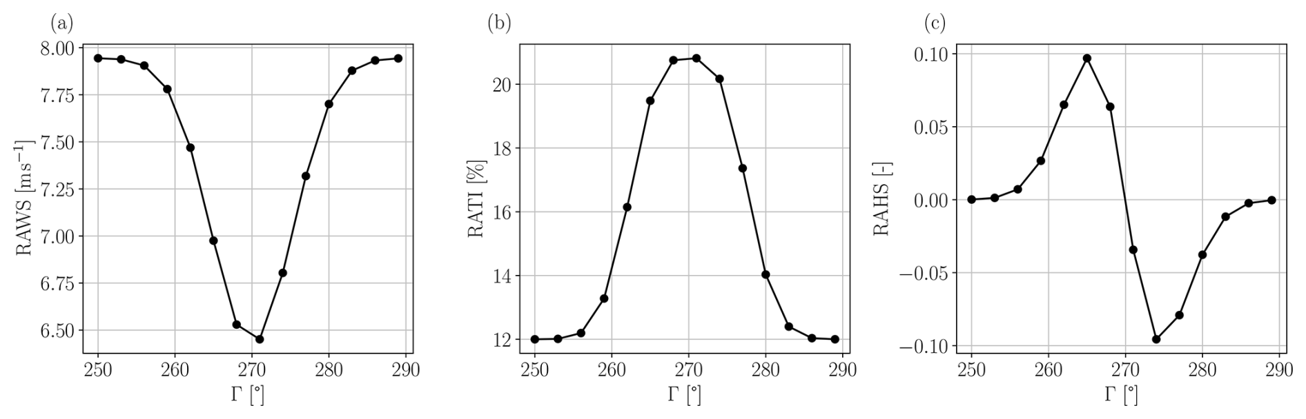
Figure A1 Variation in the RAWS (a), RATI (b), and RAHS (c) on the waked turbine of Fig. 2 for varying wind direction Γ, for an ambient wind speed of 8 m s⁻¹ and TI of 12 %. For a wind direction of 270°, the array of turbines is aligned with the incoming wind.

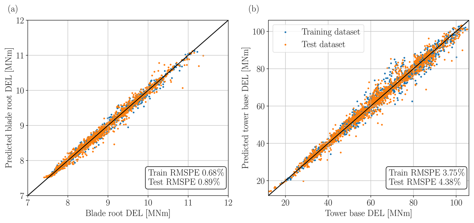
Figure A2 Performance of the load surrogate model for the projected blade root DELs (a) and projected tower base DELs (b). DELs measured on FAST.Farm (the ground truth) are on the x axis, while DELs predicted by the surrogate are on the y axis. Root-mean-square percentage errors (RMSPE) are used as performance metrics. Half of the dataset was used for the training of the ANN (in blue), while the other half was used for testing the trained ANN (in orange).

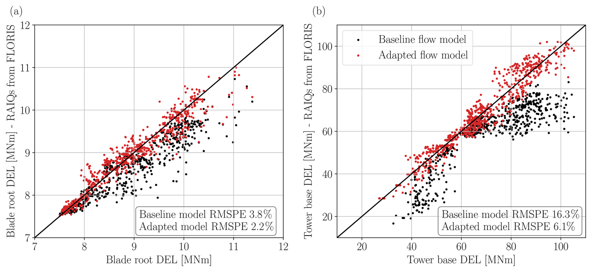
Figure A3 Comparison of DELs predicted by the load surrogate model fed by RAIQs measured on the non-calibrated FLORIS (in black) and on the calibrated version (in red). DELs measured on FAST.Farm (the ground truth) are on the x axis, while surrogate-predicted DELs are on the y axis. Data points include both the training and testing datasets for I=12 %. (a) Projected blade root DELs, (b) projected tower base DELs.

Figure A1 clearly shows that the RAWS is at its minimum for the full-wake situation (Γ=270°) and progressively recovers toward the ambient wind speed as the wind direction moves away from this value. In contrast, the RATI is largest in full-wake conditions due to wake-added turbulence. As the turbine experiences less wake impingement, the RATI decreases toward the ambient TI value. Finally, the RAHS shows the expected asymmetry, characteristic of left and right partial-waking. For both the full-wake (Γ=270°) and no-wake (Γ<255° or Γ>285°) scenarios, the RAHS is close to zero, as there is no significant wind speed asymmetry across the lateral direction of the rotor disk. However, during partial-waking situations, the RAHS is positive for $\mathrm{255}\mathit{°}<\mathrm{\Gamma }<\mathrm{270}$° and negative for $\mathrm{270}\mathit{°}<\mathrm{\Gamma }<\mathrm{285}$°. These trends in RAWS, RATI, and RAHS further contribute to the understanding of the results presented in Sect. 4.1.2.

A2 Effect of calibration on surrogate performance

Figure A2 illustrates the performance of the load surrogate model when the input RAIQs are estimated from FAST.Farm for both the training and testing datasets. The root-mean-square percentage error (RMSPE) is used as a performance metric. The scatterplots for both the training and testing datasets are similar, indicating that the ANN training data pool was sufficiently large to ensure a correct generalization.

As discussed in Sect. 3.1, load estimates based on RAIQs from FLORIS in its baseline configuration were found to be not satisfactory because of the unavoidable mismatch between its steady-state inflows and the ones generated by the dynamic model of FAST.Farm. To address this problem, the wake-added turbulence model in FLORIS was replaced with the Ishihara and Qian (2018) model, and the “wind farm as a sensor” method was used for calibrating all FLORIS model parameters from the FAST.Farm dataset (see Sect. 3.2).

To illustrate the improvements achieved by model tuning, Fig. A3 compares the DELs estimated by the load surrogate when the inflow RAIQs are computed from the non-calibrated FLORIS (shown as black dots) with the ones obtained with the calibrated FLORIS model (shown as red dots). The results show considerable improvements. In particular, panel (b) highlights the beneficial effects of flow model tuning, whereas the baseline model significantly underpredicts tower base loads. This is primarily due to the crude estimation of RATI in the baseline model, which uses the model of Crespo and Hernandez (1996).

Appendix B: Nomenclature

c	Turbine component
C	Number of turbine components
ℂ	Cost item
D	Damage
Dref	Damage threshold
𝔻	Discount rate
fa	Wind condition frequency
I	Turbulence intensity
k*	Flow model parameter
𝕂	Damage safety factor
L	Load cycle amplitude
Lu	Ultimate load
m	Wöhler exponent
n	Number of load cycles
N	Number of turbines
Neq	Equivalent number of load cycles
P	Turbine power
Pr	Turbine rated power
r	Rotor radial coordinate
𝕣	Polynomial fit parameter
R	Rotor radius
ℝ	Electricity market price
t	Time instance
T	Desired lifetime horizon
U	Wind speed
u	Control set points
Wa	Set of ambient wind conditions
𝕎	Weight parameter for load-balance strategy
y	Year
Y	Number of years in T
γ	Misalignment angle
Γ	Wind direction
Δt	Time duration
ψ	Rotor azimuthal coordinate
AEP	Annual energy production
ANN	Artificial neural network
CF	Capacity factor
DEL	Damage equivalent load
EOL	End of life
FLORIS	FLOw Redirection and Induction in Steady State
NPV	Net present value
O&M	Operation and maintenance
RAWS	Rotor-average wind speed
RATI	Rotor-average turbulence intensity
RAHS	Rotor-average horizontal shear
RAIQ	Rotor-average inflow quantity
RMSPE	Root-mean-square percentage error
TI	Turbulence intensity
WFC	Wind farm control