Experimental wind tunnel dataset of wake and turbine measurements for wind farm control

Open-access experimental datasets play a central role in validating and benchmarking numerical models used in wind energy and wind farm control research. However, publicly available datasets providing time-resolved turbine loads, actuator commands, and inflow characterization under controlled operation remain scarce.

This paper presents a newly released open-access experimental dataset from wind-tunnel experiments featuring actuated, instrumented, scaled wind turbine models. While several of the underlying experimental campaigns have supported previous publications, the data themselves are made publicly available here for the first time, in a harmonized and fully documented form. The database includes time-resolved measurements of tower-base and rotating-shaft moments, rotor speed, generated torque and power, blade pitch angles, nacelle yaw angle, and controller commands. The inflow conditions are described in terms of wind speed, wind direction, air density, and wake-flow measurements, enabling detailed analyses of turbine response and controller behavior under consistent, repeatable conditions.

The experiments cover a wide range of wake-affecting strategies, including yaw-based wake steering, curtailment and derating, Helix control, dynamic yaw actuation, Pulse wake mixing, individual pitch control for load mitigation, and several combinations of these strategies. The simultaneous availability of actuator commands, measured turbine response, and time-resolved structural loads enables detailed investigation of the controller performance, load variability, and dynamic turbine behavior induced by active wake-control strategies.

In addition to the experimental measurements, the dataset is complemented by numerical models of the experiments, providing a reproducible experimental–numerical benchmarking framework that enables dataset extension, sensitivity analyses, and systematic validation of control-oriented aeroelastic and wake-interaction models.

The dataset is intended to support the validation and benchmarking of numerical tools for wind farm control, the assessment of fatigue-relevant loading under wake-control operations, and to strengthen community efforts to improve transparency, reproducibility, and model fidelity in wind farm design and control research.

1 Introduction

Open-access experimental datasets have become a cornerstone for validation, benchmarking, and reproducibility across multiple engineering disciplines, including aeronautics, rotorcraft dynamics, and wind engineering.

In aeronautics, reference geometries and wind tunnel data – such as those of the NASA Common Research Model (Rivers and Dittberner, 2014) – have supported large-scale community benchmarking initiatives to assess the predictive capabilities of computational fluid dynamics (CFD) solvers and uncertainty quantification strategies. Coordinated efforts such as the AIAA Drag Prediction Workshops (Levy et al., 2002; Laflin et al., 2004; Levy et al., 2013; Tinoco et al., 2018; Tinoco, 2023) have demonstrated that shared experimental baselines can accelerate advances in turbulence modeling, mesh generation practices, and aerodynamic prediction accuracy. Comparable progress has been achieved within the rotorcraft community, where comprehensive experimental campaigns such as HART II (van der Wall et al., 2004) have made subsets of time-resolved aerodynamic and structural measurements publicly available. These datasets, often complemented by structured validation workshops (van der Wall, 2011; Smith et al., 2013), have contributed significantly to improvements in the modeling of unsteady aerodynamics, aeroelastic coupling, and prediction of dynamic loads.

In wind engineering, open-access datasets derived from both laboratory and full-scale measurements have long served to bridge the gap between controlled wind-tunnel conditions and the complexity of real atmospheric inflows. Publicly available measurements of wind-induced pressures, structural loads, and flow statistics, like the ones reported in Tominaga and Shirzadi (2021), Styrk Andersen et al. (2022), Shaukat and Giljarhus (2024), and Ishihara and Zhou (2025), have enabled detailed validation of numerical models, extending from mean quantities to spectral characteristics, intermittency, and extreme response events. These efforts have underscored the critical importance of time-resolved datasets for characterizing flow-structure interaction under turbulent inflow and for enhancing the reliability of predictive tools used in structural design and performance assessment (Kareem, 2010; Holmes, 2015).

The wind energy sector has particularly benefited from coordinated experimental and numerical benchmarking efforts. Laboratory-scale campaigns such as the Unsteady Aerodynamics Experiment (UAE Phase VI) (Hand et al., 2001), the MEXICO (Snel et al., 2007; Schepers et al., 2012, 2014), and New MEXICO (Boorsma and Schepers, 2014, 2016) projects have provided high-quality aerodynamic and load measurements for the validation of blade-resolved CFD and aeroelastic models. At full scale, coordinated measurement programs such as DanAero (Madsen et al., 2010) have offered valuable insight into turbine response under realistic inflow and wake conditions. In parallel, open numerical datasets and reference models released within the IEA Wind Task 37 (Bortolotti et al., 2019) have established common baselines for reproducible simulations and tool-to-tool comparison.

Despite these advances, open-access datasets specifically tailored to wind farm control and wake-interaction studies remain scarce (Veers et al., 2023). Existing experimental investigations of wake steering and active wake control often focus on aggregated power performance metrics (Doekemeijer et al., 2021; Fleming et al., 2019, 2020), and time-resolved measurements – particularly for field-scale experiments – are seldom publicly released. A case in point is the recent ambitious AWAKEN experiment (Moriarty et al., 2020), an effort of unprecedented scope and breadth that has collected extensive measurements, of which only a small fraction has ever been released to the scientific community. Moreover, available datasets – e.g., Sengers et al. (2023) and Fontanella et al. (2025) – typically emphasize wake or flow-field characterization, while detailed on-board turbine measurements under active wake-control operation are much less common if at all available outside of small closed consortia. This lack of high-resolution actuator and load data limits the validation of control-oriented load models. It also hinders the assessment of load variability arising from wake-mixing strategies.

The dataset presented in this work addresses this gap by providing a newly released open-access experimental database specifically designed for wind farm control and wake-interaction studies. The database collects measurements from several wind-tunnel campaigns conducted between 2016 and 2025; while subsets of these measurements have supported previous publications, the underlying data had never been publicly released prior to this work and are here made available in their entirety, with harmonized post-processing, uncertainty quantification, and metadata. The dataset was obtained from wind-tunnel experiments featuring small clusters of scaled, sensorized, and actuated wind turbines of the G1 type (Bottasso and Campagnolo, 2022). The measurements include time-resolved tower-base moments, rotating-shaft moments, rotor speed, generated torque and power, commanded and measured blade pitch for each blade, and nacelle yaw angle. Inflow conditions are characterized by wind speed, wind direction, air density, and wake-flow measurements, enabling comprehensive analyses of both turbine response and controller behavior under known, repeatable conditions.

The experiments cover a broad range of wake-affecting strategies, including yaw-based wake steering, curtailment and derating strategies, Helix control (Frederik et al., 2020a), dynamic yaw actuation, Pulse-based wake mixing (Frederik et al., 2020b, 2025), individual pitch control (IPC) for load reduction, and several combined strategies. By combining actuator commands, measured responses, and time-resolved structural loads, the dataset supports a detailed evaluation of controller performance, load variability, and the dynamic turbine behavior induced by active wake control.

This dataset is expected to support several research efforts: validation of control-oriented aeroelastic and wake-interaction models, assessment of load variability and fatigue-relevant statistics under wake-control operation, and benchmarking of numerical tools used for wind farm control synthesis. More broadly, it contributes to ongoing community efforts to enhance transparency, reproducibility, and model fidelity in wind farm control research.

Alongside the experimental measurements, the database provides numerical models designed to replicate the experimental setups. This combined experimental–numerical framework transforms the dataset into a reproducible benchmarking platform, enabling the extension of the database beyond the measured conditions and facilitating systematic investigations of modeling assumptions and parameter sensitivity.

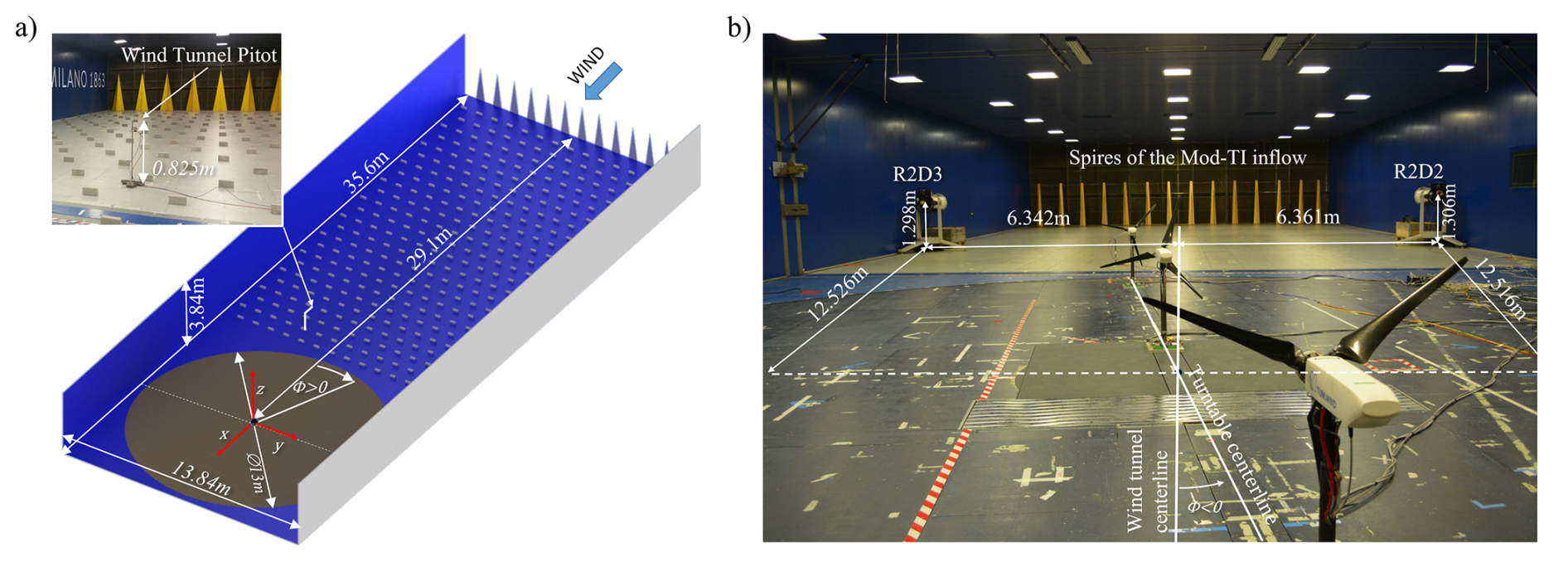
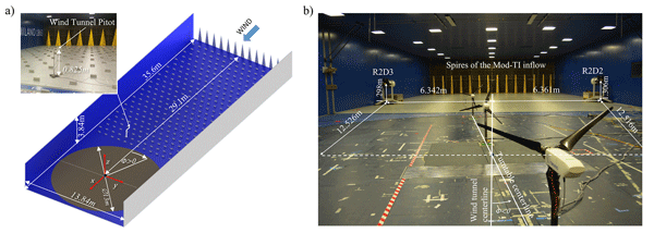
Figure 1 Main dimensions of the test section of the POLIMI wind tunnel, including the distance of the turntable center from the inlet. Wind turbine and flow-measurement device positions are measured relative to the depicted reference frame, whose origin lies at the turntable center (a). Boundary layer test section equipped with the spires used to simulate the Mod-TI inflow; note that the turntable angle Φ shown in this figure panel is negative (b).

This paper is organized as follows. Section 2 presents the experimental setup. Section 3 discusses the execution of the experiments, the data post-processing, and the expected measurement uncertainty. The experimental dataset is described in Sect. 4, while the numerical models are presented in Sect. 5. Section 6 critically discusses the scope and limitations of the dataset, i.e., what it can and cannot be used to validate. Conclusions are given in Sect. 7.

2 Experimental setup

The experiments were conducted using clusters of G1 scaled wind turbines, three-bladed machines with a rotor diameter D of 1.1 m and a hub height z_H of 0.825 m, so that the rotor spans elevations between 0.275 and 1.375 m above the floor. A complete description of the G1 model is given in Sect. 2.2; the main rotor dimensions are anticipated here to help contextualize the inflow characteristics presented in the following.

2.1 Wind tunnel

All tests were conducted in the boundary layer test section of the wind tunnel at the Politecnico di Milano (POLIMI), which consists of a closed-loop vertical conduit (Diana et al., 1998). The section, shown in Fig. 1a, is located in the return line of the facility and extends longitudinally for 35.6 m, with a width of 13.84 m and a height of 3.84 m. The test chamber is equipped with a 13 m diameter rotating table, whose center is located along the centerline, at a distance of 29.1 m from the inlet. The rotation of the table Φ, defined as positive if clockwise when viewed from above, allows simulating the effect of wind direction on the performance of the experimental setup. Φ is zero when the centerline of the turntable is aligned with the centerline of the test section, as shown in Fig. 1b. Rotation is achieved by a rubber-tired driving wheel that engages with the outer perimeter of the turntable, using the position measured by an absolute rotary encoder with 8192 pulses per revolution (PPR) as feedback. A limitation on the maximum acceleration is enforced to prevent the tire from slipping (Campagnolo et al., 2020b). The turntable rotation is measured and converted into an analog signal for acquisition by an external system.

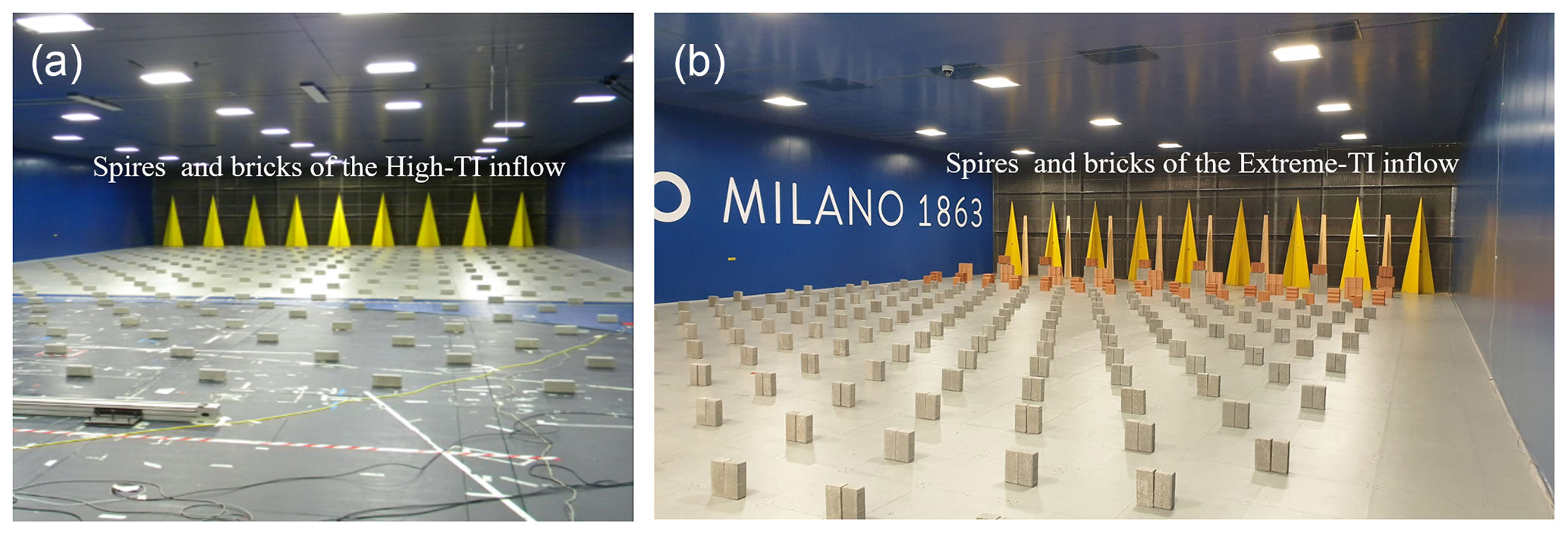
Figure 2 Spires and bricks used to simulate the High-TI boundary layer (a). Spires and bricks used to simulate the Extreme-TI boundary layer (b).

2.1.1 Boundary layer simulation

Given the relatively modest length of the test chamber compared to the dimensions of its cross-section, a proper simulation of the atmospheric boundary layer requires the installation of obstacles both at the inlet (spires, triangular or trapezoidal in shape) and on the floor (rectangular bricks) (Cermak, 2003). The size and precise position of these obstacles depend on the desired characteristics of the boundary layer, and particularly on the velocity and turbulence profiles. The dataset described in this article was obtained by reproducing four different inflows in the test section. Here and in the following, the rotor apex denotes the point of intersection at the hub of the blade pitch axes, consistent with its definition provided in Jonkman et al. (2009); Fontanella et al. (2021); Panda et al. (2025). For an untilted and not coned rotor (which is the case of the G1), the distance from the ground of the rotor apex coincides with the hub height.

• Low-TI: obtained with an empty test section; it is characterized by a low-turbulence inflow of approximately 1 %–2 % (Diana et al., 1998) and by a nearly uniform mean velocity profile across the rotor disk.

• Mod-TI: obtained by installing 14 trapezoidal spires of type A (lower base width 0.26 m, top width 0.1 m, height 2 m) at the inlet, spaced 1 m apart, as shown in Fig. 1b; it has a turbulence of about 6 % at the apex of the G1 rotor and a power-law shear exponent α ≈ 0.14.

• High-TI: obtained by installing nine type B triangular spires (base 0.8 m, height 2.5 m) at the inlet, spaced 1.55 m apart, as shown in Fig. 2a. Rectangular bricks (height 0.1 m, width 0.2 m, depth 0.06 m) are aligned diagonally on the floor, with a longitudinal and lateral spacing of 1.1 m. It has a turbulence of about 13.5 % at the apex of the G1 rotor and a power-law shear exponent α ≈ 0.21.

• Extreme-TI: obtained by installing nine type B triangular spires at the inlet, spaced 1.55 m apart and interspersed with eight type A trapezoidal spires. In addition, five different types of bricks are disposed on the floor, as shown in Fig. 2b: one row of bricks of type A (height 0.74 m, width 0.39 m, depth 0.15 m) placed immediately downstream of the spires and aligned with the spires of type A; one row of bricks of type B (height 0.5 m, width 0.4 m, depth 0.15 m) placed next, aligned with the spires of type B; one row of bricks of type C (height 0.3 m, width 0.24 m, depth 0.24 m) placed next, followed by a row of bricks of type D (height 0.24 m, width 0.22 m, depth 0.11 m), and several rows of bricks of type E (height 0.2 m, width 0.2 m, depth 0.06 m) up to the turntable. The bricks of types C, D, and E are placed diagonally on the floor at a longitudinal and lateral distance of 0.9 m. The generated inflow has a turbulence of approximately 22 % at the apex of the G1 rotor and a power-law shear exponent α ≈ 0.36.

A detailed characterization of the four inflows, including the measured vertical profiles of mean velocity and turbulence intensity, is provided in Sect. 4.1.1.

2.1.2 Wind tunnel sensors

The wind tunnel is equipped with sensors that measure the thermohygrometric parameters of the air in the boundary-layer test section. Specifically, atmospheric pressure is measured by an Effa AK-S 900-1060 transducer (uncertainty ± 0.5 hPa), temperature by a Mescon TH 12-U thermocouple transducer (uncertainty ± 0.1 % of a 100 °C full scale, i.e., ± 0.1 °C), and relative humidity (RH) with a Rense 741 transducer (uncertainty ± 2 % RH). These measurements are used to estimate the air density ρ as explained in Davis (1992).

The test section is equipped with Pitot tubes at the inlet and on the ceiling. The measurements from these sensors can be useful for controlling the wind tunnel fans, but they do not provide an accurate velocity measurement upstream of the turbine cluster being tested. For this reason, an additional Pitot tube is placed in front of the cluster, at hub height, between 3 and 4 rotor diameters upstream of the most upstream turbine. At this distance, the induction of the rotors has a negligible effect on the probe reading. The exact probe position adopted in each experiment is documented in the test matrices (see Sect. 4.3). The dynamic pressure p_dyn of the Pitot tube is measured by an MKS Baratron-Type 226A pressure transducer, characterized by an accuracy Δp_dyn = ± 0.4 Pa, and can also be acquired by external data acquisition systems. The freestream velocity representative of the undisturbed flow is then obtained as $u_{\mathrm{\infty }}=\sqrt{\mathrm{2}{p}_{\text{dyn}}/\mathit{\rho }}$.

Figure 3 Top: overview of the G1 model and its main features (Bottasso and Campagnolo, 2022). Bottom: G1 sensed quantities and corresponding reference frames. G1 with standard yaw actuator (a); G1 with fast yaw actuator (b).

2.2 Scaled wind turbine model

The wind turbine model used in the experiments, shown in Fig. 3, has a rated power P_R, torque Q_R, and rotor speed Ω_R equal to 46 W, 0.517 N m, and 850 rpm, respectively. The cut-in and cut-out velocities are 2 and 9 m s⁻¹, respectively, while the rated wind speed is around 5.8 m s⁻¹. The time compression ratio is equal to 80; i.e., time flows in the experiments 80 times faster than at full scale (Bottasso and Campagnolo, 2022). The rotor axis is parallel to the ground. The rotor is upwind, not coned, and rotates clockwise if viewed from upstream. The rotor has an overhang of 0.123 m from the tower axis. A 12-channel slip ring is used to transmit power, measurement, and control signals between the rotor and the fixed frame. The machine design process is extensively discussed in Bottasso and Campagnolo (2022). The following sections, instead, report a detailed description of the G1 hardware and software.

2.2.1 Actuators

The G1 is equipped with Maxon motors (Maxon Motor AG, 2026) that serve as pitch, yaw, and torque actuators. Each blade is individually controlled through a brushed motor DCX16L GB SL 24V, housed within the hollow root of the blade, equipped with a planetary gear-head GPX19 A (nominal gear ratio 62:1) and a co-located relative encoder ENX10 EASY (128 PPR). An EPOS2 24/2 DCX positioning controller is used to actuate the motor position. The actuation system is preloaded using a torsion spring, as described in Campagnolo (2013). This solution removes gearbox backlash, enabling the encoder to accurately measure the blade pitch; additionally, it passively sets a high blade pitch in the event of controller malfunction or power loss. The maximum pitch rate is 400 ° s⁻¹, equivalent to 5 ° s⁻¹ at full scale because of time compression. For each blade, the actuator is homed using the output of a Honeywell SS496A1 Hall-effect sensor mounted on the hub. The sensor measures the magnetic flux induced by a magnetic dipole made of two NdFeB Supermagnete Q-05-1.5-01-N magnets placed side by side. The magnets are positioned at the base of the blade and thus rotate with it. During the homing procedure, the blades are slowly rotated until the Hall sensor detects zero magnetic flux, which occurs when the sensor centerline is aligned with the magnetic dipole centerline; this triggers the encoder reset.

The torque generator consists of a brushless motor EC-4pole22 BL Y 90W KL, equipped with a planetary gear-head GP22HP 2.4 Nm 2ST KL (nominal gear ratio 14:1) and a co-located tachometer HEDL 5540 (500 PPR). An ESCON 50/5 servo-controller is used to manage the current flowing through the motor windings.

The G1 can be equipped with two different yaw actuation systems: a standard and a fast one, shown in Fig. 3a and 3b, respectively.

The standard yaw actuator, located inside the hollow tower, consists of a brushed motor DCX32L GB KL 24 V equipped with a planetary gear-head GPX37 LZ (nominal gear ratio 231:1). The nacelle position is measured by a non-co-located optical encoder US-DIGITAL E6-10000-750-IE-D-H-D-3 (10 000 PPR). An EPOS2 24/2 positioning controller, used to actuate the motor position, allows one to rotate the entire rotor–nacelle assembly at a maximum yaw rate of 20 ° s⁻¹, equivalent to 0.25 ° s⁻¹ at full scale.

The fast yaw actuation is provided by a mechanism located at the base of the tower and concealed within an airfoil-shaped cover. The mechanism, described in detail in Mühle et al. (2022), consists of a RE40 ∅ 40 mm brushed motor, a Wittenstein TK+ right-angle gearbox (nominal gear ratio 100:1) characterized by a very small backlash (γ_BL = 4 arcmin), and a co-located optical encoder HEDS 5540 (500 PPR). An EPOS2 24/5 positioning controller enables the entire rotor–nacelle assembly to rotate with a maximum yaw rate equivalent to 0.9 ° s⁻¹ at full scale.

2.2.2 Sensors

Several physical quantities are measured in the reference systems shown in Fig. 3. The blades and their corresponding actuators are numbered according to the order in which they pass through the vertical axis during a rotation. The azimuth position ψ of the first blade is measured by an optical encoder US-DIGITAL HUBDISK-2-2500-1000-IE (2500 PPR). It is defined as the angle between the vertical axis and the pitch axis, measured clockwise when looking downstream, and it is null when the first blade points upward. The pitch β_i of the ith blade is measured by the built-in encoder, and it is positive when the blade is pitched to feather. The rotation of the nacelle γ_nac is measured by the optical encoder of the yaw actuator. It is the angle between the rotor axis and the turntable centerline, positive for counter-clockwise rotation when viewed from above. The rotor speed Ω is sensed by the tachometer of the generator.

The G1 is equipped with several strain gauges arranged in full Wheatstone bridges. Two full bridges are placed close to the tower base, at a distance z_SG of 0.72 or 0.569 m from the rotor axis for the standard and fast yaw actuator, respectively. For the standard yaw actuator, the strain gauges are located below the yaw system and are therefore fixed with respect to the turntable; their sensed bending moments are noted east–west (EW, aligned with the turntable centerline) and north–south (NS, forming a right-handed triad with EW and the yaw axis). For the fast yaw actuator, the strain gauges are placed above the yaw system and therefore rotate with respect to the turntable; their sensed moments are noted side–side (SS, aligned with the rotor axis) and fore–aft (FA, forming a right-handed triad with SS and the yaw axis).

Three full bridges are placed on the rotating shaft between the rotor and the front bearing, 0.055 m from the rotor apex. They measure the main shaft torque Q_S and two out-of-plane bending moments: the moment M_y,S, aligned with the pitch axis of the first blade, and the moment M_x,S, which forms a right-handed triad with the torque and M_y,S vector.

A Lorenz Messtechnik DR2112-R torque meter (measurement uncertainty ± 0.002 N m) is used to measure the torque Q_TM supplied by the generator. Due to friction in the bearings and slip ring, the torque measured by the torque meter is smaller than the one measured by the strain gauges on the shaft, but it shows a better signal-to-noise ratio. To obtain an accurate, friction-free, low-noise measurement of mechanical torque, the following method is employed. The friction, which depends on various factors and can vary over time due to temperature and wear, is estimated by calculating the difference Q_S−Q_TM. This estimate is filtered by a high-order, low-cut-off frequency filter to eliminate noise even at low frequencies. The resulting signal is added to the torque meter measurement to compute Q_Meas, which is the torque measurement used by the control system (see Sect. 2.2.6) and logged in the machine data.

2.2.3 Sensors calibration

Before each experimental campaign, all G1 sensors are calibrated in the laboratory or in the wind tunnel, as explained below.

The load cells on the shaft and tower base are calibrated in the lab using weights whose mass is known with an accuracy of ± 0.1 g. During the calibration of the shaft sensors, the drive train is locked in four different azimuth positions; through a bar fixed to the hub, the weights are hung at varying distances from the axis of rotation to simultaneously stress the strain gauges with torsion and bending (Campagnolo, 2013). Similarly, the base of the tower is fixed to a wall, with the EW axis (or the SS axis when using the fast actuator) aligned in four directions relative to the vertical. The azimuth of the rotor and the angular position of the tower are measured with a Wyler Clinotronic PLUS inclinometer (accuracy ≤ 3 arcmin), while the load application arm with respect to the load cell is estimated from the CAD model of the G1 (accuracy ± 0.2 mm). The calibration matrix – 3 by 3 and 2 by 2 for the load cells on the shaft and tower base, respectively – is identified by least-squares using the voltage measured downstream of the entire measurement chain.

The measurement of the blade pitch is calibrated in the lab by placing the inclinometer on a CNC-machined saddle that fits onto the blade at a specific and unique span-wise location. With the blade connected to the hub and kept parallel to the ground, the blade pitch is varied using its actuator, and the inclinometer and encoder readings are recorded. The slope of their interpolating line provides a measure of the relationship between the blade pitch and the encoder pulses, yielding a more accurate estimate than one derived from the nominal gear-head ratio and the encoder PPR. The pitch at which the Hall sensor detects zero magnetic flux is also measured using the same setup.

The azimuth angle and the yaw angle in the standard yaw actuator are derived using the nominal PPR values of the corresponding encoders. When using the fast actuator, the yaw angle calculation also accounts for the gear-head nominal reduction ratio. Finally, the rotor speed is obtained using the torque actuator nominal gear ratio and encoder PPR.

As most calibration factors and matrices vary from machine to machine, they are stored on turbine-specific USB sticks. During the wind tunnel experiments, each USB stick is connected to the acquisition and control hardware of the corresponding G1. When the system boots up, the calibration parameters are acquired and stored in internal memory for real-time conversion of voltages and pulses into the corresponding physical quantities.

2.2.4 Acquisition and control hardware

Each G1 is controlled in real time by a programmable logic controller (PLC) Bachmann M1 (Bachmann electronic GmbH, 2025).

A 16-bit analog acquisition module AIO216 acquires the strain-gauge signals, appropriately conditioned by dedicated electronic boards located on the rotor and at the tower base, together with the torque-meter signal, the dynamic pressure measured by the Pitot tube transducer, and the turntable position.

An additional AIO216 module is used to provide the analog set point of the generator current to the ESCON 50/5 servo controller and to acquire the rotor speed. In particular, the generator current is managed by a control algorithm implemented on the M1, as described in Campagnolo (2013). This algorithm uses Q_Meas as feedback and regulates the generator current so that the generator supplies the torque requested by the control algorithm responsible for tracking the regulation trajectory (see Sect. 2.2.6).

The azimuth is acquired by a CNT204/R module. The blade pitch and nacelle yaw angles are transmitted by the EPOS2 in digital format via the CANopen protocol. A CM202 module is used to connect the EPOS2 to the M1 controller: it reads the pitch and yaw angles and transmits the set points β_i,Dem (the desired pitch of the ith blade) and γ_nac,Dem (the desired nacelle yaw).

The system operates at different acquisition frequencies. The M1 controller internal time, the bending moments on the shaft, the torque meter measurement, and the azimuth are acquired every 0.4 ms, i.e., with a sampling frequency f_S equal to 2.5 kHz. Conversely, the rotor speed, tower base loads, measured and demanded pitch and yaw angles, Pitot dynamic pressure, and turntable position are acquired every 4 ms (f_S = 250 Hz). The demanded curtailment or derating (see Sect. 2.2.5) is acquired every 8 ms (f_S equal to 125 Hz). The density, obtained from the wind tunnel acquisition system, is considered constant during a single test, which usually lasts a few minutes. It is therefore logged manually by the user as a scalar. The data are written to binary files on the USB stick connected to the M1.

A computer in the control room is connected via ethernet to the M1s and used to manage the machines and display the real-time measurements from the main sensors.

2.2.5 Regulation trajectories

The regulation trajectories are calculated offline using estimates of the power coefficient (C_P) provided by a simulation model of the G1 implemented in OpenFAST (see Sect. 5.4).

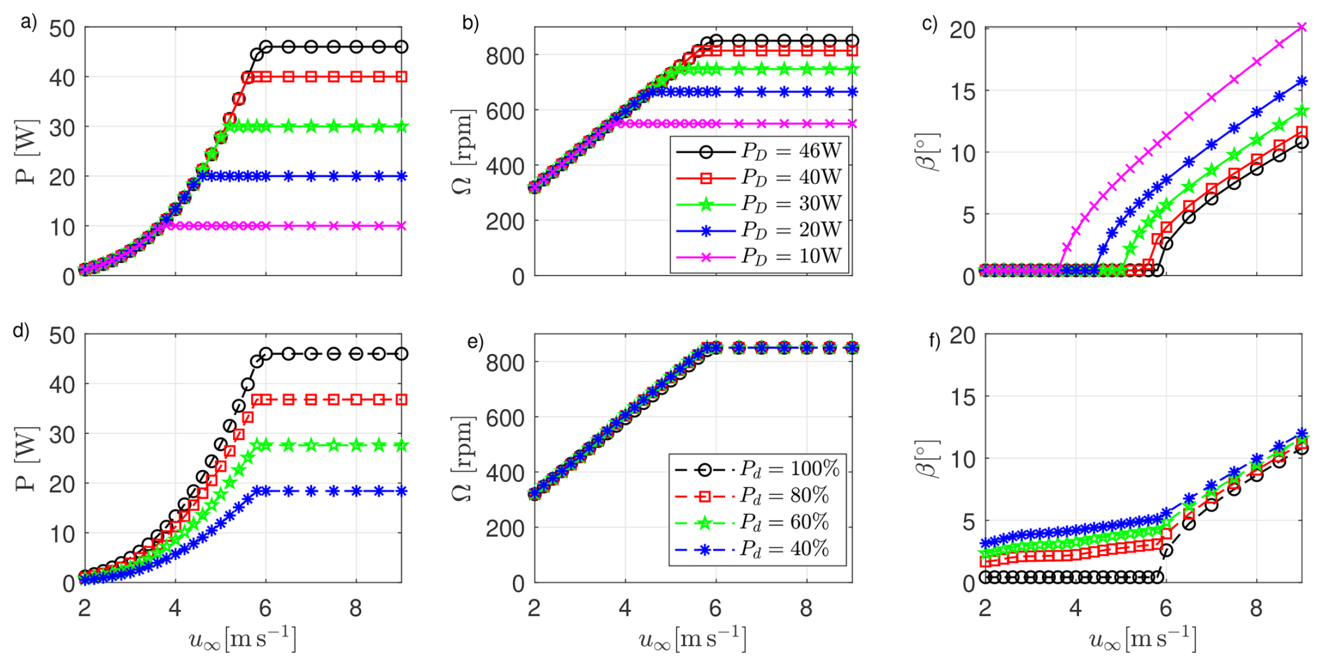
Figure 4 Regulation trajectories tracked by the G1 control algorithm with a density ρ = 1.19 kg m⁻³. The nominal regulation trajectory is depicted by black lines and circles (P_D = 46 W and P_d = 100 %). Curtailed and derated regulation trajectories are shown in panels (a–c) and (d–f), respectively.

The nominal regulation trajectory, shown in Fig. 4 using black lines and circles, maximizes the power produced by the machine for wind speeds below the rated one (region II), whereas it limits the power to the rated value P_R = 46 W for higher wind speeds (region III). The calculation of this trajectory takes into account that the power coefficient, which depends on the chord-based Reynolds number, decreases at lower wind speeds (Campagnolo et al., 2020b). Moreover, the optimal tip-speed ratio (TSR, noted λ) is set in the range 8.15–8.5, which are typical values for full-scale turbines. In region II, this results in a constant optimal pitch β_opt equal to 0.42°, a rotor speed that varies linearly with wind speed, and a torque that is scheduled as a function of the rotor speed, i.e., Q_Dem=f_Q(Ω).

The G1 can be down-regulated (or curtailed) in order to limit the power output to a given value P_D≤P_R. Among the various approaches proposed in the literature, the G1 implements the Const-Ω strategy (Lio et al., 2018). From the nominal regulation trajectory, the rotation speed corresponding to the desired power level P_D is identified and set equal to Ω_R. The resulting rated torque is $P_{\mathrm{D}}/{\mathrm{\Omega }}_{\mathrm{R}}$. Curtailed trajectories differ from the nominal one only for wind speeds higher than the value required to produce P_D, as shown in Fig. 4a–c.

The G1 can also be derated; i.e., it can deliver a power that is a fraction P_d ≤ 100 % of what is produced by following the nominal regulation trajectory, regardless of wind speed. Among the various approaches proposed in the literature (Juangarcia et al., 2018; Croce et al., 2024), the G1 strategy maintains the TSR constant. It follows that the rotor speed does not depend on derating and that the generator torque is reduced according to the derating factor, i.e., Q_Dem=f_Q(Ω)P_d. The optimal blade pitch in region II is determined by balancing electrical and aerodynamic power. Due to the dependence of aerodynamic performance on chord-based Reynolds, the desired derating in region II can only be achieved if the fine pitch varies slightly with wind speed. The plots in Fig. 4d–f show the regulation trajectories for different values of P_d, computed using the OpenFAST model of the G1.

2.2.6 Control software

The control system, developed in Simulink (The MathWorks Inc., 2023), implements closed-loop algorithms designed to track the regulation trajectories, as well as the wake-mixing strategies Helix, Dynamic Yaw, and Pulse. The control is executed on the M1 every 4 ms.

The torque and pitch controls that track the desired regulation trajectory were developed in collaboration with the National Kangwon University and are based on the work of Nam (2013). The torque control consists of a lookup table (LUT) of optimal torque for region II, scheduled based on rotor speed and derating. The torque is saturated at the rated value Q_R, which depends on the curtailment or derating. A correction term, based on a proportional-integral (PI) loop that feeds back on the error ${\mathit{ϵ}}_{\mathrm{\Omega }}=\mathrm{\Omega }-{\mathrm{\Omega }}_{\mathrm{R}}$, is added to the optimal torque to improve control behavior during the transition between below and above rated conditions. The pitch control consists of a PI loop that feeds back on ϵ_Ω, with Ω_R depending on the curtailment. The pitch is saturated at the fine value β_opt, scheduled according to the rotor speed – to account for Reynolds dependency of aerodynamic characteristics – and the derating level. A mode-switch block determines the machine operating status (above or below rated) based on filtered measurements of power, rotation speed, and blade pitch. The gains of the controllers were tuned using a numerical model of the G1 drive train and tower north–south dynamics implemented in Simulink (see Sect. 5.3). The resulting gains are K_β,P = 0.0336 s and K_β,I = 0.0168 for the pitch controller and K_Q,P = 0.00113 N m s and K_Q,I = 0.000564 N m for the torque controller. In January 2019, the integral gain of the torque controller (K_Q,I) was set to 0.00282 N m to improve the performance of the machine under conditions characterized by rapid significant changes in wind speed. This change affects only the closed-loop dynamic response of the torque controller during wind-speed transients, whereas the steady-state operating points (tip-speed ratio, power coefficient) are unaffected.

Flags are used to enable the curtailment or derating of the G1, as well as for activating the following wake-mixing strategies.

• Helix: the ith blade set point is equal to

  $$\begin{array}{}\text{(1)}& \begin{array}{rl}{\mathit{\beta }}_{i,\text{Dem}}\left(t\right)=& {\mathit{\beta }}_{\text{opt}}+{\widehat{\mathit{\beta }}}_{\text{Helix}}\sin (f_{\text{Helix}}\mathrm{2}\mathit{\pi }{f}_{\mathrm{r}}t\\ & -\mathrm{2}\mathit{\pi }/\mathrm{3}(i-\mathrm{1})),\end{array}\end{array}$$

  where ${\widehat{\mathit{\beta }}}_{\text{Helix}}$ and f_Helix are the Helix amplitude and excitation frequency, expressed in fractions of the rotational frequency f_r. A clockwise (CW) Helix is obtained if f_Helix<1, a counter-clockwise (CCW) Helix if f_Helix>1 (Mühle et al., 2024).

• Dynamic Yaw, or DY: the nacelle yaw set point is equal to

  $$\begin{array}{}\text{(2)}& {\mathit{\gamma }}_{\text{nac},\text{Dem}}\left(t\right)={\widehat{\mathit{\gamma }}}_{\text{DY}}\sin \left(\mathrm{2}\mathit{\pi }{f}_{\text{DY}}t\right),\end{array}$$

  where ${\widehat{\mathit{\gamma }}}_{\text{DY}}$ and f_DY are the DY amplitude and excitation frequency, respectively.

• Pulse, or DIC: the collective blade pitch set point is equal to

  $$\begin{array}{}\text{(3)}& {\mathit{\beta }}_{\mathrm{c},\text{Dem}}\left(t\right)={\mathit{\beta }}_{\text{DIC}}+{\widehat{\mathit{\beta }}}_{\text{DIC}}\sin \left(\mathrm{2}\mathit{\pi }{f}_{\text{DIC}}t\right),\end{array}$$

  where ${\widehat{\mathit{\beta }}}_{\text{DIC}}$ and f_DIC are the Pulse amplitude and excitation frequency, respectively, and β_DIC is the mean pitch angle.

The controller allows changing the steady yaw set point ${\stackrel{\mathrm{‾}}{\mathit{\gamma }}}_{\text{nac},\text{Dem}}$ while limiting the yaw rate to ${\dot{\mathit{\gamma }}}_{\text{max}}$. The yaw set point can be implemented even when a wake-mixing strategy is active or when the machine is curtailed/derated, thus combining wake steering with wake mixing or induction control.

Finally, load reduction is achieved through an individual-pitch-control (IPC) algorithm (Bossanyi, 2003). The IPC scheme is based on two PI controllers that feed back on the projections of the shaft loads M_y,S and M_x,S onto a fixed reference frame. The resulting load signals are properly filtered using a low-pass filter prior to control action. Finally, the control request accounts for the delay introduced by the pitch actuator dynamics, as described in Petrović and Campagnolo (2013).

2.3 Hot-wire CTA probes

Flow measurements were carried out using tri-axial hot-wire CTA Dantec 55R91 probes, consisting of three fiber-film sensors, each perpendicular to the others. The sensors form an orthogonal system with an acceptance cone of 70.4° and are connected to a six-channel Dantec StreamLine Pro anemometric system. The latter is connected to a National Instruments PXI System (National Instruments, 2024), which samples the data at 0.5 ms (f_S = 2 kHz) and stores them in internal memory.

The hot-wire probes are calibrated in an open-circuit wind tunnel of the Aerodynamics Laboratory at POLIMI (Politecnico di Milano, 2025), whose test section is 150 mm wide and 200 mm high. The inlet contraction ratio is 25, while the maximum speed is 100 m s⁻¹. The wind tunnel flow velocity is calculated by measuring the dynamic pressure with a pressure transducer DRUCK LPM9481 (accuracy ± 0.5 Pa), while the density is derived from the measurement of the atmospheric pressure, relative humidity, and temperature. The probe is mounted on its support, whose attitude with respect to the wind tunnel flow is measured by a dual-axis inclinometer SPECTRON L-212T (accuracy ± 0.3°). The probes are calibrated with respect to Reynolds number and velocity direction. The calibration procedure accounts for the effects of flow temperature, relative humidity, and absolute pressure, as described by Raffel et al. (2011).

Measurements in the boundary-layer test section are performed using two probes supported by a double-pronged sting. The latter, in turn, is attached to a two-axis traversing system, as shown in Fig. 5 and is precisely aligned to the inflow direction using an inclinometer. This setup enables automated movement of the probes along the vertical and lateral axes. The traversing system can be positioned anywhere within the test section, allowing the mapping of the undisturbed inflow or of the wake shed by the scaled wind turbines. The position of each probe within the traversing system is measured using the encoders present in the electrical motors of the two linear actuators. Given the position of the traversing system, it is possible to reconstruct the position of the probes with respect to the reference system shown in Fig. 1a. The three speed components u_x, u_y, and u_z of the velocity vector u are measured in the reference system shown in Fig. 5.

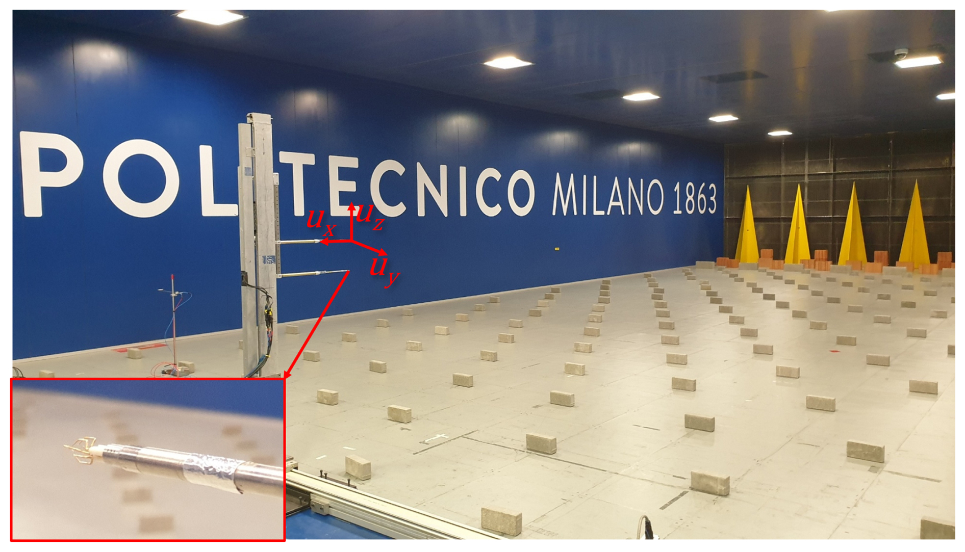
Figure 5 Traversing system equipped with two CTA probes, each one measuring the three components of the velocity vector u along the longitudinal (u_x), lateral (u_y), and vertical (u_z) directions.

2.4 Lidars

Measurements of the undisturbed inflow and of the wakes shed by three G1s were also taken using two short-range WindScanner lidars (Mikkelsen et al., 2012), named R2D2 and R2D3. The lidar head scans were positioned as shown in Fig. 1b: R2D2 at x = −12.516 m, y = 6.361 m, z = 1.306 m; R2D3 at x = −12.526 m, y = −6.342 m, z = 1.298 m. Each lidar measures v_LOS, i.e., the projection of u on the lidar line of sight, with a sampling frequency f_S = 390 Hz. The two time- and space-synchronized measurements of v_LOS provided by the lidars are used to estimate the u_x and u_y components of the wind speed. The experimental setup, its calibration, the data acquisition, and its post-processing are described in detail in van Dooren et al. (2017). For the dataset described in this article, the measurements were resampled at f_S = 250 Hz.

3 Execution of the wind tunnel experiments, data post-processing, and measurement uncertainties

This section describes the procedures followed during the execution of the experiments, including the assembly of the experimental setup, the zeroing of the sensors, the synchronization of the data, their post-processing, and, finally, the estimation of measurement uncertainties.

3.1 Assembly of the experimental setup

The experimental setup, including the G1 wind turbines, the Pitot tube placed upstream of the cluster, and, when necessary, the CTA probes with their traversing system or the lidars, is assembled in the test section at the beginning of an experimental campaign, and possibly later modified as necessary depending on the test matrix. The assembly is carried out with the rotating table set to zero degrees. The entire setup is positioned at the desired locations, defined by their coordinates [$x,y,z$] in the reference system shown in Fig. 1a. To this aim, a longitudinal line parallel to the inflow direction is traced onto the floor of the test section using a multi-line laser level Huepar LS41G positioned at the center of the turntable. Using a measuring tape, points are marked at the x coordinates. Centering the laser level at these points, transverse lines are drawn, on which points are marked at the y coordinates. When positioning the wind speed sensing probes, the laser level is centered at the coordinates [x,y], and the head of the Pitot tube or the CTA probe is placed at the desired z coordinate using a measuring stick. The laser level is also used to align the G1 base with the incoming inflow. For information on lidar positioning, please see van Dooren et al. (2017).

The G1 turbines are mounted on heavy steel interface plates (thickness: 25 mm, mass > 100 kg) that are, in turn, fixed to the wooden floor of the turntable. Experimental verification confirmed that this mounting configuration does not affect the model natural frequencies. The PLCs that control the G1s, the traversing control system, and the acquisition system of the CTA probes are positioned inside the test chamber, close to the side walls and therefore sufficiently distant (at least 4–5 D) from the experimental setup. Their impact on the flow impinging on the G1s and on the wakes they shed is negligible.

3.2 Zeroing the sensors

Most of the G1 sensors and other sensors (CTA probes, turntable position, etc.) are reset when there is no wind in the test section, and the rotating table is set to 0°. Specifically, the G1 pitch actuator encoder is reset when the PLC is started or rebooted, using the homing procedure described in Sect. 2.2.1. The encoder that measures the nacelle yaw is reset as follows. Once the G1 installation is complete, the yaw actuator is moved until the index channel is detected by its encoder. At this point, the encoder is reset, and the actuator is moved in the opposite direction until the rotor axis is precisely aligned with the inflow direction, using the multi-line laser for the purpose. The yaw angle read by the encoder in this condition is then saved on the G1 USB stick. Each time the PLC is started, an automated homing procedure is performed: (i) the yaw is varied until the index is detected, (ii) the nacelle is then rotated in the opposite direction by an angle equal to the value stored on the USB stick, and (iii) the encoder is reset.

Some sensors are subject to measurement drift and must be frequently reset, usually before and after each test run. The torque meter, the Pitot transducer, the analog signal that carries the turntable position, and the CTA probes are reset with the G1 actuators disabled. The sensors at the tower base are reset by keeping the nacelle yaw at zero (γ_nac = 0°) and the rotor standing still. The tower loads are therefore corrected for the gravitational loads induced by the masses of the tower and rotor–nacelle assembly in the configuration γ_nac = 0°. The load induced by the rotor–nacelle assembly is particularly significant, given that its center of gravity is quite offset from the tower axis. The load sensors on the shaft are reset as follows: several rotor rotations are performed at very low speed (Ω < 30 rpm), with the load cell measuring solely zero-mean gravitational loads. The average values read by the sensors are stored in internal memory and subtracted from subsequent measurements in real time.

The encoder that reads the azimuth is reset via software every time its index channel is detected. Once the G1 has been assembled in the wind tunnel, the rotor is manually rotated a few times to ensure that the index channel is detected. The rotor is then set to zero azimuth using a laser level. The value of ψ in this position is stored on the USB stick and subtracted in real time from subsequent measurements.

The zeroing of hot-wire probes is performed with the wind tunnel off. For the reset of the lidars, please see van Dooren et al. (2017).

3.3 Test execution and data synchronization

The tests are conducted according to a specific test matrix. Once the desired environmental conditions (wind speed and turntable angle) and the operating conditions of the G1s (control type and related settings) have been set, a few seconds are allowed for the wakes to develop and for the response of the machines to stabilize. Data acquisition then proceeds for the required duration.

The data acquired from the G1s are synchronized as follows. A MATLAB script, executed on the computer that manages the G1s, simultaneously sends a request to start acquisition on all M1s via the Modbus protocol; the maximum expected desynchronization is less than 10 ms. Synchronization between G1 and CTA probe data is achieved by orally synchronizing the start of the respective acquisitions; the expected desynchronization is on the order of 1 s. Synchronization between G1 and lidar data is achieved through postprocessing: during the experiments, the acquisition systems of the upstream G1 and the lidars both acquire the same trigger signal, generated by a third source; the maximum expected desynchronization is less than the sample time, i.e., 4 ms.

3.4 Data post-processing

The binary data of the G1s and of the flow probes are converted into the format presented in Sect. 4.2 and saved to NetCDF files using MATLAB scripts. Most measurements are saved as they are recorded. The measurements of rotor speed and shaft torque are instead first filtered using a forward–backward eighth-order low-pass Butterworth filter (pass-band equal to 3 times the average rotational frequency), and then saved in the NetCDF files. Power is calculated as the product of these two physical quantities, with the torque downsampled to 250 Hz.

3.4.1 Post-processing of flow measurements

Post-processing of the hot-wire probe data consists of transforming, via the calibration matrix, the voltages measured by the acquisition system into the three velocity components. The resulting data are then corrected as follows. At the beginning of a measurement campaign, the flow is sampled along a horizontal line at hub height without the turbines installed in the wind tunnel, i.e., under conditions such that the mean flow can be considered aligned with the longitudinal direction. For each acquisition point, the yaw angle ${\mathit{\gamma }}_{\mathit{u}}=\text{atan2}(u_y,u_x)$ and the tilt angle ${\mathit{\phi }}_{\mathit{u}}=\text{atan2}(u_z,\sqrt{u_x^{\mathrm{2}}+u_y^{\mathrm{2}}})$ of the mean velocity vector are computed. Any deviation from zero is attributed to imperfect leveling of the measurement system – including the traversing unit, the probes, and their support – rather than to small elastic deformations during motion. During post-processing, the average yaw and tilt estimated in this preliminary scan are subtracted from the corresponding angles measured during the campaign. The time history of the velocity vector is then reconstructed. This correction assumes that the yaw and tilt biases are stationary throughout the measurement campaign and independent of the flow conditions, which is reasonable given the relatively low wind speeds of the test. This assumption was verified by quantifying the variability in the yaw and tilt biases for different wind speeds within the range of the tested ones, which was found to be within ± 0.1°, i.e.,  within the ± 0.2° uncertainty quoted for the hot-wire flow angles in Sect. 3.6. For the post-processing of the lidar data, please see van Dooren et al. (2017).

3.4.2 Post-processing to compensate for strain-gauge torque drifts

In a few experiments at sub-rated wind speeds, discrepancies of up to 15 % of Q_R were observed between measurements of Q_S at two consecutive zeroings due to malfunctioning of the strain gauges conditioning boards. This indicates a drift in the measurement chain during data acquisition, compromising the accuracy of the mechanical torque signal. Because this signal is used as feedback by the generator current controller (see Sect. 2.2.2), the actual generator torque deviates from the target value Q_Dem by a quantity comparable to the drift. Consequently, G1 settles at a rotational speed – and thus a TSR – different from the intended operating point. This leads to operation at a C_P different from the expected value and to an inaccurate computation of the reference torque. A simple algebraic correction of the measured torque by adding or subtracting the estimated drift is therefore not sufficient. The thrust coefficient C_T, on the other hand, is only marginally affected, owing to its low sensitivity to TSR in region II.

In such cases, torque and speed measurements were corrected during post-processing as follows. A Simulink model of the drive-train and tower NS dynamics (see Sect. 5.3) was used to perform simulations with turbulent wind fields with mean speeds between the cut-in and rated values. The generator torque was artificially biased within ± 15 % Q_R to reproduce the effect of the drift on the closed-loop dynamics. For each simulation, differences in the mean mechanical torque and rotational speed with respect to the unbiased case, denoted ΔQ and ΔΩ, were stored in a LUT parameterized by the imposed bias and the mean rotational speed. The drift during each experiment was estimated assuming it varies linearly with time and then used, together with the measured rotational speed, to interpolate the LUT. The interpolated values were finally used to correct the measured torque and speed. The resulting time series are filtered as explained above, and then saved in the NetCDF files.

A comparison between experiments conducted under the same environmental and operating conditions, some with torque signal drift and others without, highlighted the validity of the developed correction method, even in the presence of significant drift. In particular, the measured power is consistent with variations within the expected measurement uncertainty. For experiments affected by torque signal drift, however, there is a discrepancy between the rotation speed recorded in the data and the rotation speed that can be calculated by differentiating the azimuth or inferred from the shaft load spectrum.

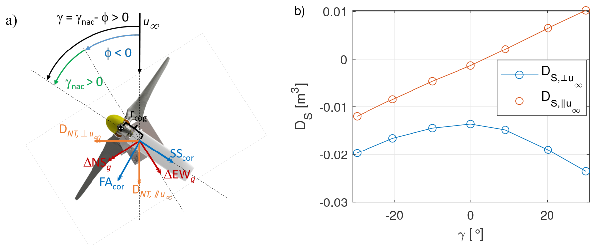
Figure 6 Schematic of the thrust calculation (a). Drag static moments of the G1 nacelle and tower as a function of the yaw misalignment (b).

Only a small portion of the experimental dataset was affected by torque-signal drift. The affected experiments, to which the above correction is applied, are explicitly flagged in the test matrices accompanying the datasets (see Sect. 4.3), so that users are always aware of whether they are working with corrected data. It is also noted that the correction depends solely on the estimated torque drift – derived from the data recorded during the sensor zeroing performed before and after each test – and on the rotational speed. As long as the machine operates in region II, the correction therefore applies regardless of whether the G1 operates in free stream or in the wake of an upstream turbine.

3.4.3 Post-processing to compensate for rotor imbalances

The G1 rotor exhibits small but non-negligible inertial and aerodynamic imbalances. The inertial imbalance originates from minor mass asymmetries among the blades and from the non-uniform azimuthal and radial distribution of wiring in the hub region (see Fig. 3, top). The aerodynamic imbalance reflects both deviations of the blade geometry from the nominal profile due to manufacturing tolerances (Campagnolo, 2013) and the uncertainty in blade pitch measurement (see Sect. 3.6) used as feedback by the pitch actuator, resulting in slightly different pitch settings among the blades. These imbalances affect the bending moments measured on the rotor and tower: the mean rotor-side moments deviate from zero, whereas the tower-base moments exhibit a pronounced component at the rotational frequency (f_r, or 1P). The measurements are corrected as follows. The shaft-side moments are first projected onto a fixed reference frame using the rotor azimuth; the 1P component is then removed by demodulating the time series over a moving window spanning one rotor revolution; the corrected moments are finally projected back onto the rotating frame. Tower-base moments are similarly corrected for the 1P component by demodulating the raw signals. Both the original and corrected loads are stored in the NetCDF files.

3.5 Derivable physical quantities

The signals measured during the experiments can be used to derive other physical quantities.

At a fixed wind-tunnel fan rotational speed, the mean wind speed measured by the Pitot probe may vary slightly between tests due to the turbulent nature of the flow. For this reason, the turbine performance is usually analyzed in terms of normalized power, defined as $P_{\mathrm{n}}=\mathrm{2}\stackrel{\mathrm{‾}}{P}/\left(\mathit{\rho }A{\stackrel{\mathrm{‾}}{u}}_{\mathrm{\infty }}^{\mathrm{3}}\right)$, where $\stackrel{\mathrm{‾}}{P}$ is the mean mechanical power measured at the shaft, A is the rotor disk area, and ${\stackrel{\mathrm{‾}}{u}}_{\mathrm{\infty }}$ is the mean Pitot wind speed. The normalized power of the upstream turbine (WT1) corresponds to its power coefficient, C_P. For the downstream turbines operating in the wake, the normalized power differs from C_P, as discussed in Campagnolo et al. (2020b).

The moments measured on the rotating shaft can be projected onto the fixed reference frame, thus obtaining the nodding (tilt) moment Nod_F and the yawing moment Yaw_F acting on the nacelle. These moments are stored in the NetCDF files after being corrected for the effects of the inertial and aerodynamic imbalance of the rotor and for the contribution of the rotor weight.

The moments measured at the tower base can be used to estimate the thrust coefficient, defined as $C_{\mathrm{T}}=\mathrm{2}\stackrel{\mathrm{‾}}{T}/\left(\mathit{\rho }A{\stackrel{\mathrm{‾}}{u}}_{\mathrm{\infty }}^{\mathrm{2}}\right)$, with $\stackrel{\mathrm{‾}}{T}$ the mean thrust along the rotor axis. Estimating $\stackrel{\mathrm{‾}}{T}$ is also possible if the rotor is yawed, and requires correcting the loads for (i) the yaw-dependent drag of the nacelle and tower and (ii) the variations in gravitational loads for γ_nac≠0°.

With reference to Fig. 6a, the moments induced by the nacelle and tower drag along directions, respectively, parallel and perpendicular to u_∞, are expressed as

$$\begin{array}{}\text{(4a)}& {\displaystyle }{D}_{\text{NT},\parallel u_{\mathrm{\infty }}}& {\displaystyle }={\displaystyle \frac{\mathrm{1}}{\mathrm{2}}}\mathit{\rho }{u}_{\mathrm{\infty }}^{\mathrm{2}}{D}_{{\mathrm{S}}_{\parallel u_{\mathrm{\infty }}}}\left(\mathit{\gamma }\right),\text{(4b)}& {\displaystyle }{D}_{\text{NT},⟂u_{\mathrm{\infty }}}& {\displaystyle }={\displaystyle \frac{\mathrm{1}}{\mathrm{2}}}\mathit{\rho }{u}_{\mathrm{\infty }}^{\mathrm{2}}{D}_{{\mathrm{S}}_{⟂u_{\mathrm{\infty }}}}\left(\mathit{\gamma }\right),\end{array}$$

where the drag static moments $D_{{\mathrm{S}}_{\parallel u_{\mathrm{\infty }}}}$ and $D_{{\mathrm{S}}_{⟂u_{\mathrm{\infty }}}}$ are reported in Fig. 6b. Both quantities depend on the misalignment angle, which is defined as $\mathit{\gamma }={\mathit{\gamma }}_{\text{nac}}-\mathrm{\Phi }$, with positive γ corresponding to a counter-clockwise misalignment when viewed from above. The drag static moments were obtained experimentally by measuring the moments at the tower base with the blades removed, and for several misalignment angles.

Yawing the nacelle also modifies the gravitational loads sensed at the tower base relative to the aligned condition γ_nac = 0°. Their variation is

$$\begin{array}{}\text{(5a)}& {\displaystyle }\mathrm{\Delta }{\text{NS}}_{\mathrm{g}}& {\displaystyle }=W{r}_{\text{cog}}(\cos {\mathit{\gamma }}_{\text{nac}}-\mathrm{1})\approx a_{\text{NS}}{\mathit{\gamma }}_{\text{nac}}^{\mathrm{2}},\text{(5b)}& {\displaystyle }\mathrm{\Delta }{\text{EW}}_{\mathrm{g}}& {\displaystyle }=W{r}_{\text{cog}}\sin {\mathit{\gamma }}_{\text{nac}}\approx a_{\text{EW}}{\mathit{\gamma }}_{\text{nac}},\end{array}$$

where W is the total rotor–nacelle weight, r_cog the distance of its center of gravity from the tower axis, and γ_nac the nacelle yaw angle expressed in degrees. The coefficients a_NS and b_NS were obtained experimentally, yielding a_NS = −1.7 × 10⁻⁴ N m and a_EW = 1.832 × 10⁻² N m.

Given the measured tower-base bending moment vector $\mathit{m}=[\text{NS};\text{EW}]$, the gravitational correction vector term $\mathrm{\Delta }{\mathit{m}}_{\mathrm{g}}=[\mathrm{\Delta }{\text{NS}}_{\mathrm{g}};\mathrm{\Delta }{\text{EW}}_{\mathrm{g}}]$, and the nacelle-tower drag contribution ${\mathit{d}}_{\text{NT}}=[D_{\text{NT},⟂U_{\mathrm{\infty }}};D_{\text{NT},\parallel U_{\mathrm{\infty }}}]$, the corrected tower-base bending moment vector is readily computed as

$$\begin{array}{}\text{(6)}& {\mathit{m}}_{\text{cor}}=\mathit{m}-\mathrm{\Delta }{\mathit{m}}_{\mathrm{g}}-\mathbf{R}\left(\mathit{\varphi }\right){\mathit{d}}_{\text{NT}},\end{array}$$

with R(⋅) denoting the 2D rotation matrix.

The projection of the corrected loads onto a reference frame aligned with the rotor axis yields

$$\begin{array}{}\text{(7)}& {\mathit{m}}_{\text{RA},\text{cor}}=\mathbf{R}(-\mathit{\gamma }){\mathit{m}}_{\text{cor}},\end{array}$$

with ${\mathit{m}}_{\text{RA},\text{cor}}=[{\text{FA}}_{\text{cor}};{\text{SS}}_{\text{cor}}]$. The thrust is finally obtained as $T=-{\text{FA}}_{\text{cor}}/z_{\text{SG}}$, with z_SG the elevation of the rotor axis above the strain-gauge section (see Fig. 3, bottom).

If the fast yaw actuator is used, the reconstruction is considerably simplified. In this case, the sensors at tower base rotate with the nacelle and are already corrected for gravitational loads during their zeroing (see Sect. 3.2); no additional gravitational correction is therefore required. The corrected fore–aft and side–side moments are obtained as

$$\begin{array}{}\text{(8)}& {\mathit{m}}_{\text{RA},\text{cor}}={\mathit{m}}_{\text{RA}}-\mathbf{R}(-\mathit{\gamma }){\mathit{d}}_{\text{NT}},\end{array}$$

with ${\mathit{m}}_{\text{RA}}=[\text{FA};\text{SS}]$ the raw tower-base bending moment vector.

Previous publications (Campagnolo et al., 2020b; Campagnolo and Bottasso, 2021; Campagnolo et al., 2022a; Mühle et al., 2024) have investigated damage equivalent loads (DELs) collected on the G1 turbine. Therein, the DELs are calculated using the rainflow counting algorithm implemented in MATLAB (The MathWorks Inc., 2023) and the Palmgren–Miners rule (Miner, 1945). The equivalent number of cycles is defined as the product of the load signal duration and the rated rotor speed of the nominal regulation trajectory (Ω_R = 850 rpm). In this way, it is possible to directly compare DELs calculated from time histories of different durations. The slope of the S-N curve is set to m=10 for tower-based loads and hub loads projected onto the fixed frame and m=4 for rotating loads, as the latter are assumed to be representative of the fatigue loads experienced by composite blades. For computing the DELs, load signals are filtered above 6 times the rotor frequency (6P) to remove high-frequency load components. Combined DELs may also be obtained by projecting the two orthogonal load components on the direction associated with the maximum DEL. Finally, normalized DELs are computed as ${\text{DEL}}_n=\mathrm{2}\text{DEL}/\left(\mathit{\rho }AR{\stackrel{\mathrm{‾}}{u}}_{\mathrm{\infty }}^{\mathrm{2}}\right)$.

The torque, Nod_F and Yaw_F moments can be used to estimate the rotor effective wind speed (REWS) and the effective wind speed on four equally sized, 90° wide sectors, as described in Schreiber et al. (2020b). For this purpose, it is necessary to use a mapping of the power and cone (C_m, defined in Bottasso et al., 2018) coefficients, which can be derived using the OpenFAST model of the G1 (see Sect. 5.4). A validation of this method against lidar data is discussed in Campagnolo et al. (2017).

3.6 Assessment of the measurement uncertainties

The sensors of the experimental setup measure physical quantities affected by uncertainty, classifiable according to their respective sources, namely the following.

• Linearity: associated with the linearity of the calibration model. In this work, the standard deviation of the residuals with respect to the calibration line is used to estimate the uncertainty, consistent with the guidelines of ISO and OIML (1993).

• Resolution: due to the discrete nature of the measurement output. Assuming a uniform quantization error over the interval $[-\mathit{\delta }/\mathrm{2},+\mathit{\delta }/\mathrm{2}]$, the resulting uncertainty for a 95 % confidence level is $\mathrm{\Delta }=\mathrm{1.645}\mathit{\delta }/\left(\mathrm{2}\sqrt{\mathrm{3}}\right)$, as prescribed in ISO and OIML (1993).

• Thermal drift: mainly associated with temperature-induced variations in the sensor output at zero-load (temperature effect on zero, or TEZ).

• Zeroing: type B standard uncertainty associated with the definition of the zero position.

• Backlash: the yaw encoder of the fast actuation system measures angular position upstream of a gearbox that exhibits mechanical backlash equal to γ_BL. Consequently, the encoder reading does not uniquely define the yaw angle in the presence of directional reversals, giving rise to a deadband-type uncertainty for a 95 % confidence level equal to $\mathrm{\Delta }=\mathrm{1.645}{\mathit{\gamma }}_{\text{BL}}/\sqrt{\mathrm{3}}$.

• Other: contributions not included in the categories above.

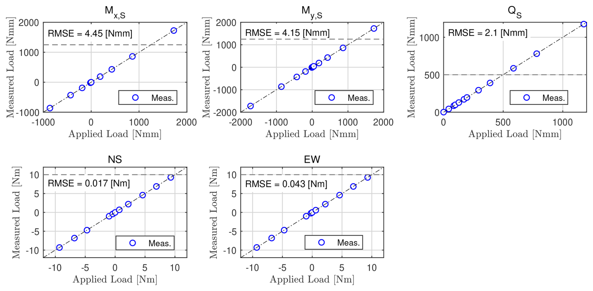
Figure 7 Comparison between applied loads (x axis) and loads reconstructed using the calibration matrix (y axis). The horizontal dashed lines mark the absolute value of the expected loads at the rated wind speed. The plots include the 1:1 reference (dash-dotted line) and the RMSE of the residuals.

G1 load transducers are predominantly affected by linearity uncertainty. Figure 7 compares the applied loads (x axis) with those reconstructed through the calibration matrix (y axis) of a G1 unit. The root-mean-square error (RMSE) shown in the plots is used as an estimate of the linearity uncertainty at the intended confidence level. Similar results have been observed across multiple G1 units.

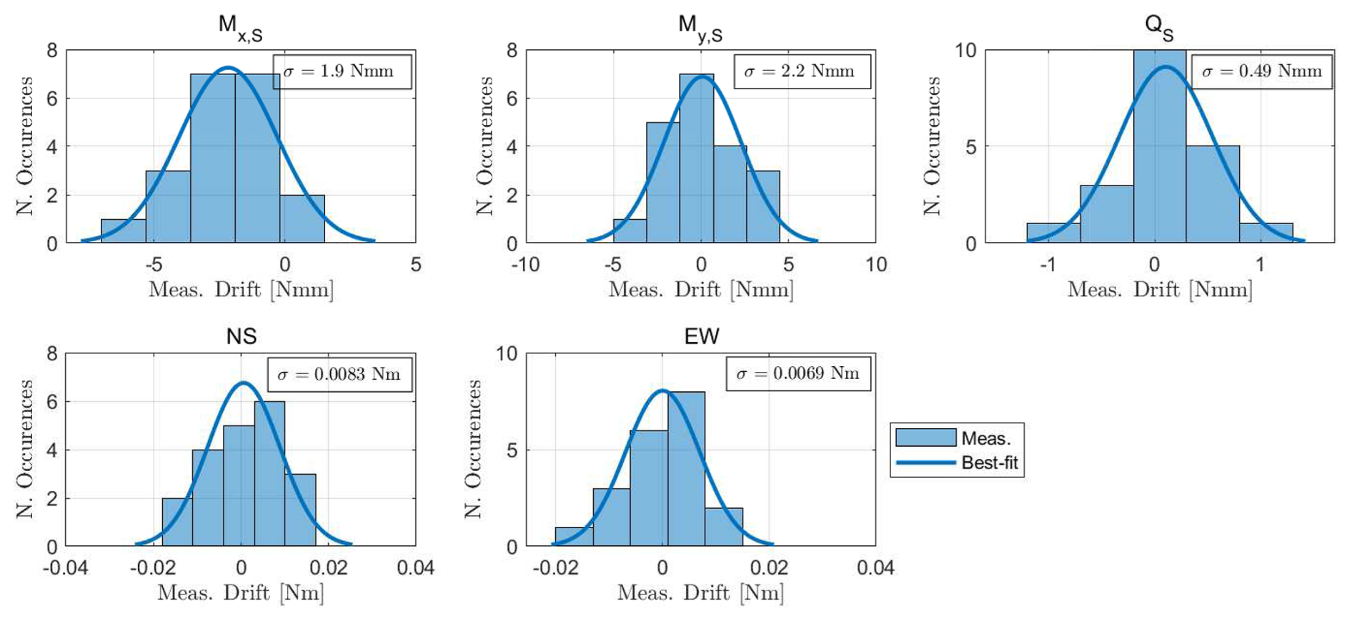
Figure 8 Distribution of the zero drift of the five G1 load sensors between successive zeroing. The plots also include the best-fitting Gaussian, with its standard deviation reported within the text box.

An analysis performed over multiple successive zeroings of the load cells indicated a small thermally induced drift in the transducer zero, which may lead to inaccurate measurements, as explained in Sect. 3.4. Figure 8 reports the distribution of the variation in the zero offsets between two consecutive zeroing procedures of a G1 unit. The standard deviation obtained from the Gaussian fits is used to quantify the uncertainty at the chosen confidence level. Similar results have been observed across multiple G1 units.

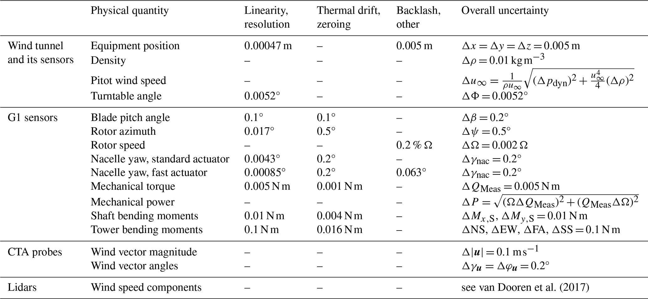
van Dooren et al. (2017)

Table 1 Uncertainty summary table at a 95 % confidence level. For selected physical quantities, the table reports the uncertainty contributions from linearity, resolution, thermal drift, zeroing, backlash, and other sources.

Encoder-based measurements are primarily affected by resolution uncertainty. Let N_p denote the PPR of the encoder and i the reduction ratio of any gearbox interposed between the encoder and the body whose rotation angle is to be determined; the corresponding angular resolution is then given by $\mathit{\delta }=\mathrm{360}\mathit{°}/\mathrm{4}{N}_{\mathrm{p}}i$, as the CNT204/R and EPOS2 24/2 modules implement X4 encoding.

For the encoder measuring the pitch angle, the linearity uncertainty is evaluated from the residuals with respect to the best-fit calibration line obtained from encoder-inclinometer measurements (see Sect. 2.2.3). The resulting RMSE is typically on the order of 0.05°.

The G1 encoders require a zeroing procedure (see Sect. 3.2). The yaw-control and azimuth encoders are zeroed in the wind tunnel using a laser level, with an estimated accuracy on the order of 0.2–0.5°. The pitch encoders are instead zeroed using a Hall sensor calibrated in the laboratory (see Sect. 2.2.3). Several repetitions of the calibration procedure indicate a repeatability of 0.1°.

The positioning of the devices installed in the wind tunnel is performed using a meter (1 mm resolution) and a laser level (see Sect. 3.1). Repeated positioning tests reveal small variations in the device's actual location, which is therefore considered known with an uncertainty of 5 mm.

The uncertainty associated with measuring the rotor angular velocity warrants special consideration. For some G1s, the angular velocity obtained by differentiating the azimuth encoder signal slightly differs from that measured by the torque-actuator encoder. This discrepancy is attributable to a small deviation (up to 0.2 %) of the gearbox reduction ratio from its nominal value, due to manufacturing tolerances, and constitutes the dominant source of uncertainty. Since the rotor speed is obtained from the torque-actuator encoder through the nominal reduction ratio (see Sect. 2.2.3), this deviation translates directly into a relative uncertainty of up to 0.2 % on the rotor angular velocity, i.e., about 1.7 rpm at the rated speed of 850 rpm.

Derived physical quantities inherit uncertainties by propagation of the uncertainties in the underlying measured variables. For the density, this results in an expected uncertainty of Δρ = 0.01 kg m⁻³.

The uncertainty associated with hot-wire probe measurements under laminar conditions is discussed in Raffel et al. (2011). In turbulent flows, the same authors estimate an uncertainty of 0.1 m s⁻¹ on the velocity magnitude |u|, and 0.2° on the tilt and yaw angles. Finally, the uncertainty associated with the lidar measurements is described in detail in van Dooren et al. (2017).

Table 1 provides a summary of the measurement uncertainties at a 95 % confidence level. For selected physical quantities, the table reports the uncertainty contributions arising from the sources discussed above. The overall uncertainty (last column) is conservatively estimated as the sum of the individual contributions when these are of comparable magnitude or as the maximum contribution when one source is dominant. The arithmetic sum is deliberately preferred over the root-sum-of-squares combination, which would be appropriate only under the assumption of statistically independent contributions. Since such independence cannot always be guaranteed, the arithmetic sum provides a conservative upper bound of the overall uncertainty.

4 Experimental dataset

This section describes the content of the experimental dataset, the data format, and the provided metadata.

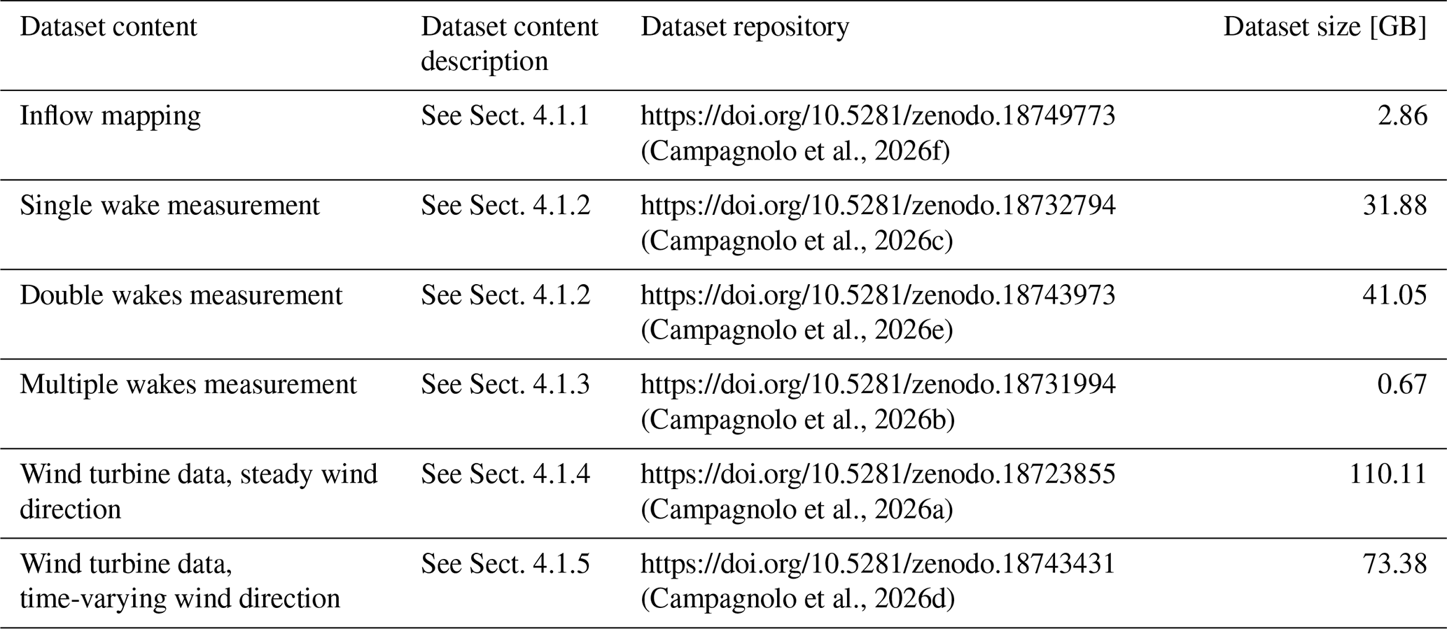
(Campagnolo et al., 2026f)(Campagnolo et al., 2026c)(Campagnolo et al., 2026e)(Campagnolo et al., 2026b)(Campagnolo et al., 2026a)(Campagnolo et al., 2026d)

Table 2 Overview of the data content included in the experimental dataset, corresponding description, repository, and dataset size.

4.1 Dataset content

The content of the experimental dataset is summarized in Table 2. It includes experimental inflow mappings obtained in an empty test section, wake measurements downstream of one, two, or three turbines, and turbine operational data measured for a three-turbine cluster under both stationary and dynamically varying mean wind-direction conditions.

The measurements were collected over several wind-tunnel campaigns conducted between 2016 and 2025. For each dataset, the following sections summarize the experimental conditions regarding inflow, wind farm layout, and tested control strategies, complementing the machine-readable test matrices described in Sect. 4.3.

4.1.1 Inflow mapping with empty wind tunnel

Measurements of the inflow were performed with the four ABLs presented in Sect. 2.1.1. The Low-TI was sampled using the lidars along a vertical plane at the turntable center point. The Mod-TI, High-TI, and Extreme-TI ABLs were sampled with the CTA probes 9.94 m upstream of the turntable center point. The inflow mapping was performed along a vertical plane for the Mod-TI and High-TI ABLs, and along a vertical and a horizontal line at hub height for the Extreme-TI.

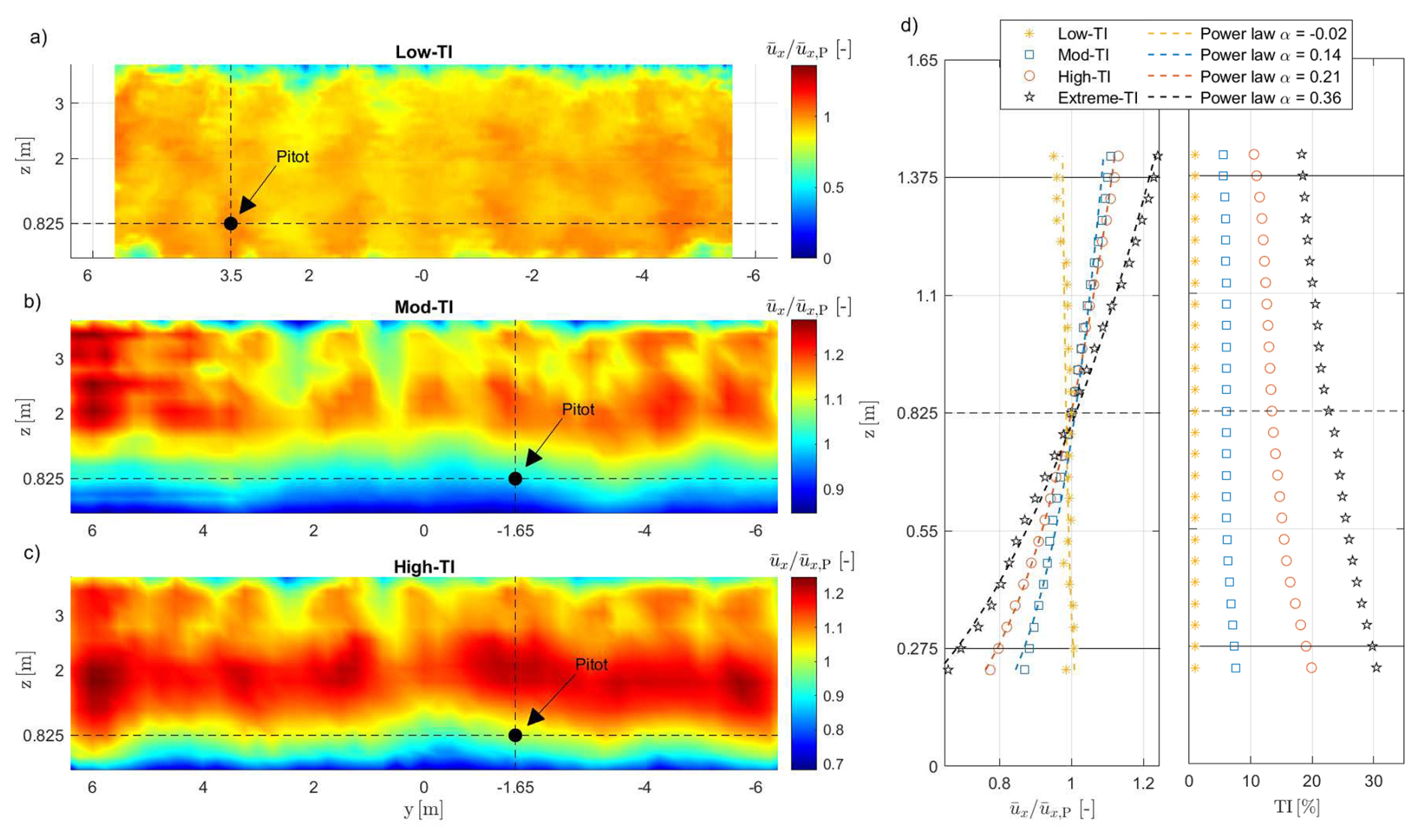
Figure 9 Characteristics of the inflows that were passively generated in the wind tunnel and measured by the lidars or CTA probes: normalized longitudinal wind velocity with Low-TI (a), Mod-TI (b), and High-TI (c) inflows, looking downstream; vertical profiles of the normalized longitudinal wind speed and their best-fitting power laws (d, left), and vertical profiles of the longitudinal turbulence intensity (d, right); within (d), the dashed black line indicates the hub height, while the two solid black lines limit the rotor disk.

The dataset (Campagnolo et al., 2026f) consists of time histories of the three velocity components measured by the CTA probes, along with lidar measurements of the mean longitudinal velocity. Figure 9a–c show the mean longitudinal velocity ${\stackrel{\mathrm{‾}}{u}}_x$ for the Low-TI, Mod-TI, and High-TI ABLs, normalized by the mean longitudinal velocity ${\stackrel{\mathrm{‾}}{u}}_{x,\mathrm{P}}$ measured at the reference Pitot position. Figure 9d shows the vertical profiles, measured at the pitot position, of the normalized longitudinal velocity (left) and longitudinal turbulence (right).

The non-homogeneity of the mean flow is evident not only in the vertical direction but also across the transverse direction, as previously discussed in Schreiber et al. (2020c); Campagnolo et al. (2020b, 2022b). Experimental measurements indicate that this non-homogeneity is only marginally affected by the operating power of the wind tunnel fans, at least within the velocity range relevant to the G1 experiments. Therefore, the inflow mapping can be scaled by multiplying the ratio ${\stackrel{\mathrm{‾}}{u}}_x/{\stackrel{\mathrm{‾}}{u}}_{x,\mathrm{P}}$ by the mean velocity measured at the Pitot location during the G1 experiments.

The inflow mapping was used to normalize G1 power production in Campagnolo et al. (2020b), whereas it was applied to wake normalization in Wang et al. (2017a).

4.1.2 Measurement of single and double wakes with CTA probes

The wake generated by a single G1 or by a tandem of two G1 turbines was measured using CTA probes. Wake measurements were performed along horizontal lines and, for the single-wake experiments, also along vertical lines, at various downstream distances from the rotor(s).

In summary, the single-wake dataset comprises 201 experiments, performed under all four ABLs described in Sect. 2.1.1, with the G1 operating in region II at freestream hub-height wind speeds between approximately 5 and 6 m s⁻¹. The tested control conditions comprise baseline greedy operation, static yaw misalignments between −40 and +40°, power curtailment with set points down to about 37 % of the greedy reference, Pulse operation – realized through sinusoidal collective pitch oscillations with frequencies between 0.5 and 2.3 Hz, corresponding to Strouhal numbers $\mathit{St}=fD/u_{\mathrm{\infty }}$ between approximately 0.1 and 0.45, and amplitudes up to 6.5° – and IPC for load mitigation. The wake was surveyed at longitudinal distances from 2 D to 10 D downstream of the rotor, along horizontal lines at hub height, and along vertical lines passing through the wake center.

The double-wake dataset comprises 68 experiments, also performed under all four ABLs, with two G1s in tandem at longitudinal spacings of 3.2 D, 4.1 D, and 5 D, in the latter case also with a lateral offset of the downstream machine of 0.5 D. The tested control conditions comprise baseline greedy operation, wake steering with a yaw misalignment of 30° applied to the upstream machine, to the downstream machine, or to both, and power curtailment of the upstream machine, in some cases combined with a deep curtailment of the waked downstream machine. In this case, the wake was surveyed at longitudinal distances between 5 D and 11 D downstream of the most upstream rotor, along a single horizontal line at hub height or, in a subset of experiments, along three horizontal lines located at hub height and at 0.36 D above and below it.

The datasets (Campagnolo et al., 2026c, e) consist of time histories of the three velocity components measured by the CTA probes, along with time series of the corresponding operational data for the G1 turbine(s). These data have been used for the development (Kim et al., 2018; Schreiber et al., 2020a; Zengler et al., 2024) and validation (Schreiber et al., 2017; Ruisi and Bossanyi, 2019; Campagnolo et al., 2019; Schreiber et al., 2020c) of wake engineering models, for the tuning and validation of large-eddy simulation (LES) codes (Wang et al., 2017a, b, 2019), and for assessing the impact of IPC and wake mixing techniques on wake recovery (Wang et al., 2020a, c).

4.1.3 Measurement of multiple wakes with lidars

The wake generated by a cluster of three G1 turbines, arranged in a column with longitudinal and lateral spacings of 4 D and 0.5 D, respectively, was measured using lidars along a horizontal plane located approximately 0.1 m above the hub height.

This dataset comprises four 10 min experiments at a freestream hub-height wind speed of approximately 5.7 m s⁻¹: one baseline run with all machines in greedy operation, and three wake-steering runs with yaw misalignments $({\mathit{\gamma }}_{\mathrm{1}},{\mathit{\gamma }}_{\mathrm{2}})=(\mathrm{7}\mathit{°},\mathrm{5}\mathit{°})$, (14°,11°), and (20°,16°) applied to the upstream and central turbines, while the most downstream machine was always aligned with the mean flow.

The dataset (Campagnolo et al., 2026b) consists of time series of the line-of-sight, longitudinal, and lateral velocity components measured by the lidars, together with the corresponding operational data of the G1 turbines. These data have been used to assess the reliability of lidar measurements in boundary-layer wind tunnels (van Dooren et al., 2016; van Dooren et al., 2017) and to validate LES codes (Draper et al., 2018a, b; Wang et al., 2018a, 2020d).

4.1.4 Wind turbine data under steady wind direction

Measurements of G1 operational data were performed using a cluster of three turbines arranged in a column, with inter-turbine spacings ranging from 4 D to 5 D. Data were collected under the three atmospheric boundary-layer conditions Low-TI, Mod-TI, and High-TI. During each experimental run, the mean wind speed and direction were held constant, and multiple tests were performed to assess the cluster sensitivity to variations in these parameters.

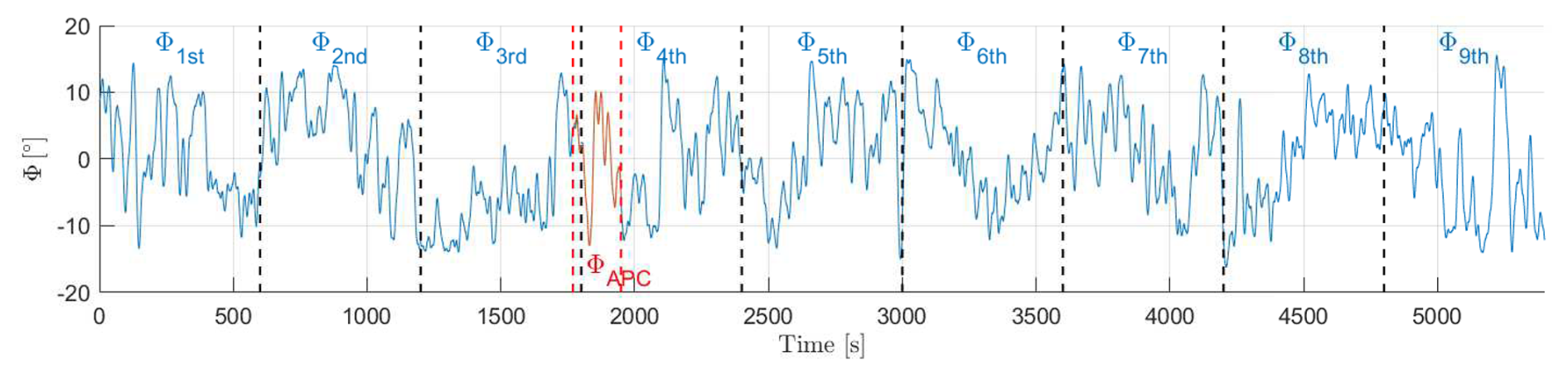
Figure 10 The 90 min time history of the rotation imposed on the turntable during experiments with dynamically varying wind direction. The 10 min blocks used for the power-boosting experiments are shown in blue and are separated by vertical dashed black lines. The 180 s block used for the APC experiments, labeled Φ_APC, is shown in red.

In summary, this dataset comprises 1650 experiments, with typical durations between 60 and 300 s, collected in several campaigns between 2016 and 2025. The turntable angle was varied between −11.5 and +11.5° to emulate different mean wind directions, and the freestream hub-height wind speed ranged between approximately 2.8 and 7.5 m s⁻¹, covering operation from region II up to above-rated conditions. The tested control settings comprise static yaw misalignments of the upstream and central turbines between ± 40°; power derating of one or more machines with levels between 50 % and 90 % of the available power, also in combination with wake steering; active power control of the cluster, with the same open- and closed-loop APC variants described in Sect. 4.1.5, here operated under steady wind direction; Pulse operation, with collective pitch oscillation frequencies between 0.5 and 2.3 Hz and amplitudes up to 7°; Helix operation, in both the clockwise and counter-clockwise variants, with excitation frequencies between 0.025 and 0.3 times the rotor frequency and amplitudes between 1 and 4°, also in combination with wake steering; dynamic yaw actuation with amplitudes between 2 and 20° and frequencies between 0.5 and 2.25 Hz; and IPC for load mitigation.

The dataset (Campagnolo et al., 2026a) has been used to investigate the effectiveness of several wake-control techniques (Campagnolo et al., 2016, 2023; Wang et al., 2020c; Frederik et al., 2020b; Bortolin et al., 2026; Mühle et al., 2026), to develop and validate engineering models of wind farms (Schreiber et al., 2017; Draper et al., 2018b; Schreiber et al., 2020c; Campagnolo et al., 2020b, 2022b), and to develop models that capture the effect on power of the way a turbine is controlled as it is misaligned (Tamaro et al., 2024).

4.1.5 Wind turbine data under dynamically varying wind direction

Measurements were performed using a cluster of three G1 turbines arranged in a column with a spacing of 5 D, with the turntable dynamically rotated to reproduce time-varying wind-direction conditions. Figure 10 shows the 90 min time history of the rotation imposed on the turntable, synthesized to reproduce wind-direction variations observed in real atmospheric conditions (Campagnolo et al., 2020b).

The G1 operational data were collected by testing two classes of control strategies. The first class consists of LUT-based wind farm control algorithms aimed at boosting cluster power through wake steering. The second class comprises active power control (APC) algorithms (Tamaro et al., 2026) that track a prescribed time-varying reference power level by a combination of curtailment and yaw misalignment. In the former case, the tests were conducted by dividing the wind-direction time history into nine blocks of 10 min, as shown in Fig. 10, and by using LUTs computed as described in Campagnolo et al. (2020b). In the latter case, the tests lasted 180 s and were conducted using a portion of the 90 min time history, highlighted in red and labeled Φ_APC in Fig. 10. In both cases, filtered measurements of wind direction were fed to the controllers to determine, in real time, the optimal control settings.

In summary, this dataset comprises 264 experiments. In the power-boosting experiments, the tested wake-steering configurations cover several LUT synthesis approaches – based on the FLORIS engineering model, on an augmented version thereof, or on a purely data-driven approach, as well as variants restricted to positive yaw offsets or including an actuation threshold – together with LUTs robustified against wind-direction uncertainties in standard deviation σ_ϕ = 2, 4, and 6°; the wind-direction signal fed to the controllers was filtered with moving averages of 1.5, 7.5, or 15 s. In the APC experiments, open-loop and closed-loop APC variants (the latter also with load-balancing and maximum-margin options) tracked normalized power references of 0.8, 0.85, and 0.9, realized by curtailment alone or combined with yaw misalignment; in this case, the wind direction was filtered with a first-order low-pass filter with a 0.25 Hz cut-off frequency.

Table 3 Structure of the NetCDF files storing the G1s, hot-wire CTA probe, and lidar data.

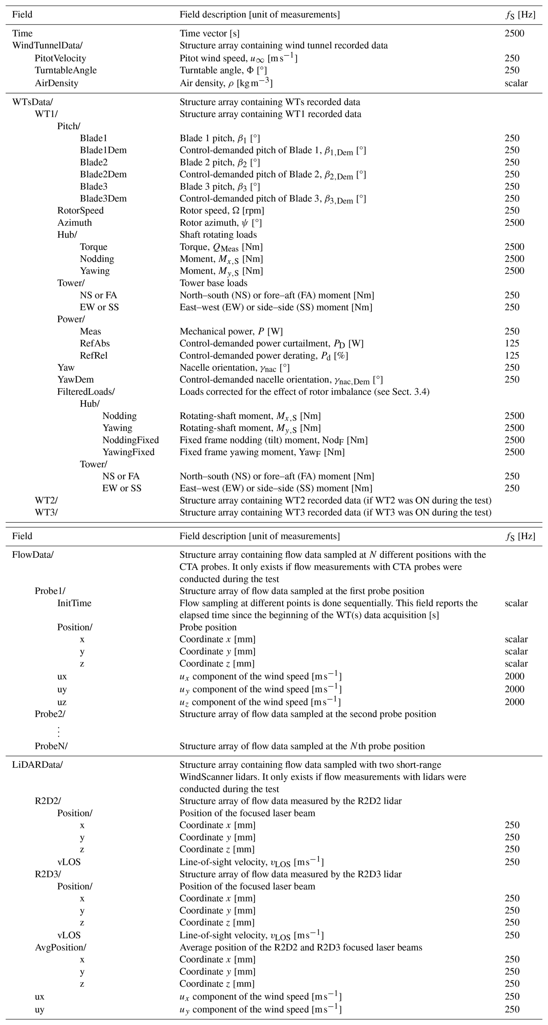
The dataset (Campagnolo et al., 2026d) consists of time series of operational data from the G1s, as well as the LUTs of the power-boosting wind farm controller. The APC controllers are provided in Tamaro et al. (2025). The data have been used in several research works (Campagnolo et al., 2020a, b; Campagnolo and Bottasso, 2021; Tamaro et al., 2026) to study the effects of control settings on the power production and fatigue loads of the turbine cluster.

4.2 Data format

The data are saved in NetCDF files using the structure described in Table 3. In addition to the measurements from the sensors described in the previous sections, the time elapsed since the start of data acquisition, sampled at 2.5 kHz, is also saved.

For signals sampled at frequencies other than 2.5 kHz, the corresponding time histories can be reconstructed by downsampling the time vector to match the signal sampling frequency. Data acquired from the most upstream machine in the cluster are stored in the substructure WT1. For tests involving two or more G1 turbines, data from the central and most downstream machines are stored in the substructures WT2 and WT3, respectively.

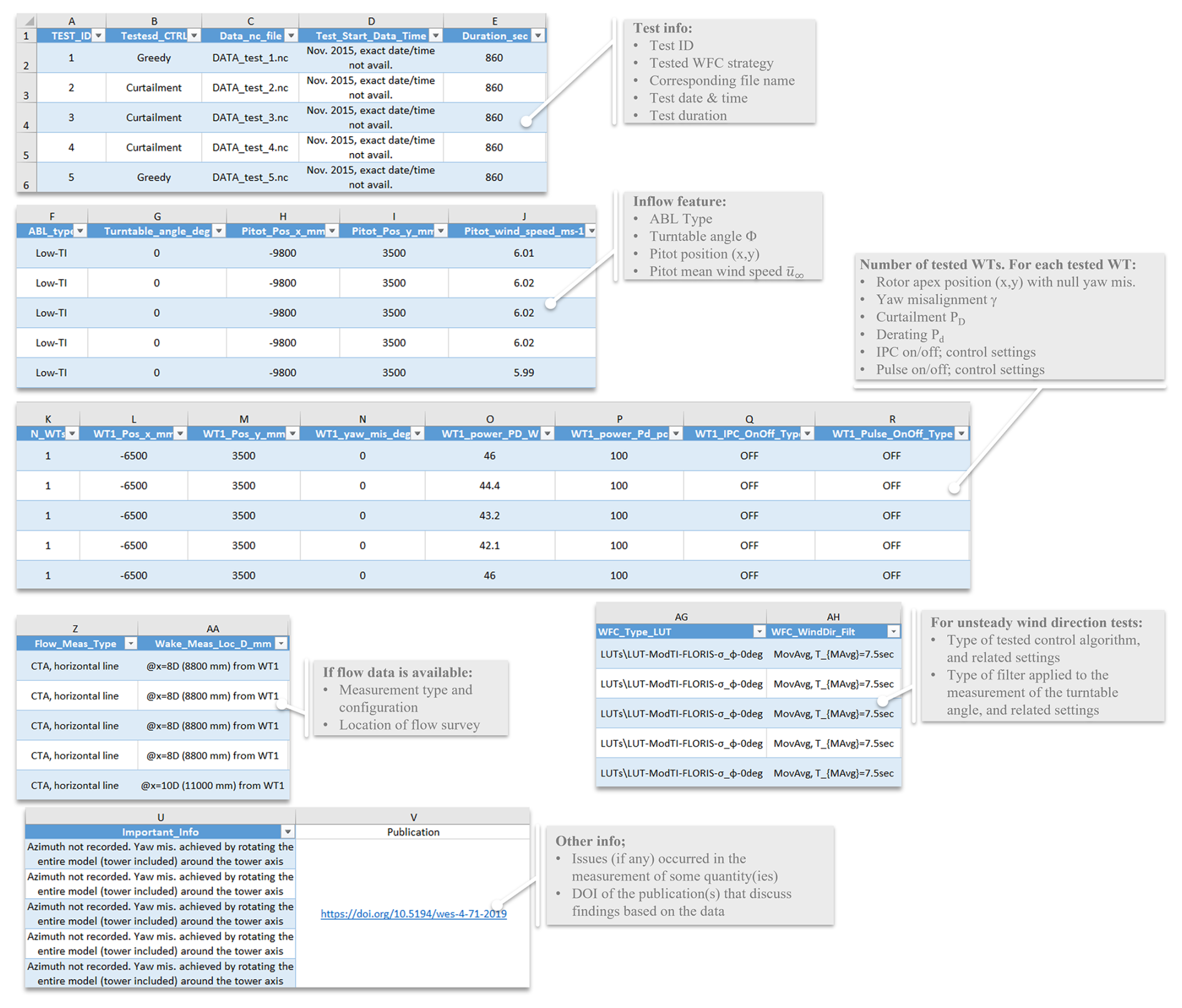
Figure 11 Test matrix summarizing all wind-tunnel experiments included in the corresponding dataset. For each experimental run, the matrix reports the test identifier, the tested wind farm control strategy, the execution date and time, the main inflow conditions reproduced in the wind tunnel, the wind farm layout and turbine positions in the test section, the turbine-level control settings, and the availability and configuration of any dedicated wake measurements. Each entry in the test matrix uniquely identifies the associated data file and provides the reference metadata required to interpret and compare the measurements across different experimental conditions.

4.3 Metadata

Each dataset is accompanied by its own test matrix (Fig. 11) that provides a compact systematic overview of all wind-tunnel experiments included in the corresponding data release. The test matrix is intended as a reference tool to support the interpretation, selection, and comparison of the measurements across different experimental conditions.

Each entry of the test matrix corresponds to a single experimental run and uniquely identifies the associated data file, ensuring a one-to-one correspondence between the experimental metadata and the stored measurement time series. For each test, the matrix documents the execution date and time and the wind farm layout adopted in the wind tunnel, including the number of G1s and their relative positions within the test section, expressed in the reference frame of Fig. 1. The main characteristics of the inflow conditions reproduced during the experiment are also reported, including the simulated ABL, the turntable angle, the Pitot tube position, and its mean wind speed.

The test matrix further specifies the wind farm control strategy applied in each experiment. This includes the class of control algorithm under investigation and the corresponding control settings assigned to each turbine, such as static or dynamic yaw offsets, power curtailment or derating, and amplitude and frequency of the Helix or Pulse control. This information allows controlled cases to be clearly distinguished from baseline (greedy) operation and enables consistent comparisons across different control strategies.

For experiments that include dedicated flow measurements, the test matrix indicates the availability of these data and summarizes the associated measurement configurations, including the measurement technique and the location of the flow surveys. This facilitates the identification of test cases suitable for wake-related analyses and the correct interpretation of flow-field data in relation to turbine operating conditions.

For experiments with dynamically changing wind direction, the test matrix reports the applied control algorithm and settings, as well as the filter used to process the measured turntable angle. Additionally, it reports any issues that occurred with one or more sensors during data acquisition, as well as previous publications that present findings derived from the data analysis.

(Campagnolo et al., 2026i)(Campagnolo et al., 2026k)(Campagnolo et al., 2026l)(Campagnolo et al., 2026g)(Campagnolo et al., 2026h)(Campagnolo et al., 2026j)

Table 4 Overview of the provided numerical models, corresponding software, description, and repository.

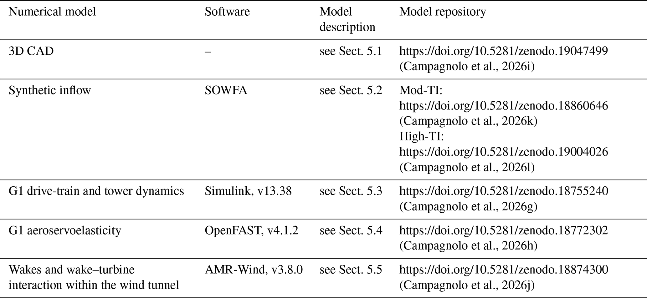
Since the completeness and clarity of a data description can ultimately only be assessed by its users, the repository documentation (README files and test matrices) will be maintained and updated in response to community feedback, exploiting the versioning capabilities of Zenodo, which preserve the citability of each release through versioned DOIs. Users are warmly encouraged to report issues, ambiguities, or suggestions for improvement to the corresponding author.

5 Numerical models

The experimental dataset is complemented by a set of numerical models for four main reasons. First, the models document in a machine-readable form the geometric, structural, aerodynamic, and control characteristics of the scaled turbines and of the wind-tunnel environment, which is essential information for any independent modeling effort. Second, they lower the entry barrier for new users of the dataset, who can start from a working reference implementation. Third, they provide a verified baseline against which independently developed models can be checked, before being validated against the experimental data. Fourth, they enable the reproduction of the results, which is one of the pillars supporting integrity, error verification, and trust building in scientific research. It should be emphasized that these models are optional companions to the data, and not prescriptive choices: since no model is perfect, users are explicitly encouraged to develop, test, and validate their own independent implementations against the experimental measurements, thereby avoiding the bias that would result from the community converging on a single modeling chain.

The numerical models, listed in Table 4, simulate different aspects of the G1 wind-tunnel experiments. Two of the provided models focus on the aeroservoelastic behavior of the G1 turbines and do not explicitly resolve the wakes generated in the wind tunnel or their interaction with downstream machines. One of the numerical models, instead, explicitly accounts for wake development and wake–turbine interactions within the wind-tunnel environment. A synthetic representation of the inflow conditions imposed in the wind tunnel, used as input to the numerical simulations, is also provided. Finally, three-dimensional CAD models of the G1 turbine are provided for two configurations: with the standard and with the fast yaw actuator.

The numerical models can complement the experimental dataset by predicting physical quantities that were not directly measured during the experiments (e.g., loads, deflections, and accelerations of G1 components, and flow-related quantities), thereby supporting a more comprehensive interpretation of the investigated phenomena. Furthermore, the models provide a framework for assessing innovative control techniques and for validating supporting technologies prior to wind-tunnel testing.

A validation of the models using a subset of the experimental data described in Sect. 4.1 is presented in Appendix A.

5.1 Three-dimensional CAD model

The three-dimensional CAD models are simplified representations of the G1 geometry that retain the machine external shape. The provided data (Campagnolo et al., 2026i) consist of two STEP (.stp) files representing the nominal geometry of a G1 turbine characterized by a collective blade pitch equal to β_opt = 0.42°, i.e., the fine pitch of the nominal control trajectory in region II; zero rotor azimuth (ψ=0); and zero nacelle yaw angle (γ_nac=0).

These CAD geometries are suitable for generating conformal meshes for blade-resolved CFD simulations. It should be noted that, owing to manufacturing tolerances in the blade production process, minor discrepancies may exist between the nominal G1 blade geometry and the actual geometry of the tested blades, which is not known.

5.2 Synthetic inflow

Time histories of the synthetic inflows generated by two LES analyses, aimed at reproducing the Mod-TI and High-TI atmospheric boundary layers (ABLs), are provided. The simulations were performed using the Simulator fOr Wind Farm Applications (SOWFA, Churchfield et al., 2012), including an explicit representation of the spires and roughness elements used to generate the boundary layer in the wind tunnel. Further details of the numerical setup are reported in Wang et al. (2019).

The provided datasets (Campagnolo et al., 2026k, l) consist of time histories of the three velocity components sampled along a vertical plane located 19.1 m downstream of the inlet, i.e., 10 m upstream of the turntable center, and therefore very close to the location of the corresponding experimental inflow mapping. For the Mod-TI case, the time history spans approximately 70 s, with data sampled at 0.9 ms intervals. For the High-TI case, the time history spans approximately 40 s, with data sampled at 1 ms intervals. For each time instant, a text file is provided in the corresponding folder containing the three instantaneous components of the velocity vector sampled at the mesh nodes. The coordinates of the mesh nodes are specified in a separate file.

The synthetic inflow can be scaled following the same procedure suggested for the experimental inflow mapping, described in Sect. 4.1.1. The resulting inflows have been used in several studies (Wang et al., 2017a, 2018b, a, 2019, 2020d, a, c, 2021; Bortolin et al., 2026; Mühle et al., 2026) to numerically assess the impact of a wide range of wind farm control strategies on the performance of a cluster of G1 turbines and their shed wakes.

5.3 Simulink model

A two-degree-of-freedom (2-DOF) numerical model of the G1 turbine is implemented in Simulink. The model neglects blade and drivetrain flexibility and resolves the drivetrain and north–south tower dynamics, the latter represented by a mass-spring-damper system.

For aligned operation (γ = 0°), the rotor aerodynamic power and thrust are computed using blade element momentum (BEM) theory, as implemented in the OpenFAST model described in Sect. 5.4. Specifically, simulations were performed for multiple combinations of wind speed, tip-speed ratio, and collective blade pitch. The resulting aerodynamic power and thrust coefficients are stored in three-dimensional LUTs, which are interpolated in Simulink during model execution.

The model can also predict power and thrust losses induced by yaw misalignment. To this end, the approach proposed in Tamaro et al. (2024) is adopted, which accounts for the effect of yaw misalignment on rotor aerodynamic performance as collective pitch, tip-speed ratio, rotor speed, and vertical shear vary. The corresponding thrust and power loss factors, η_T and η_P, are stored in five-dimensional LUTs and interpolated during model execution. These loss factors are applied to the thrust and power predicted under aligned conditions.

The 2-DOF numerical model includes the controller responsible for tracking the prescribed control trajectory, also during curtailed or derated operation (see Sect. 2.2.6). The temporal evolution of wind speed is defined by the REWS estimated from the appropriately scaled synthetic inflow.

The provided model (Campagnolo et al., 2026g) consists of a Simulink file and its parameters, available in a MATLAB (.mat) file. The model has been used, in its original or slightly modified form, to support research on wind-turbine and wind farm control strategies (Campagnolo et al., 2022a; Tamaro et al., 2026).

5.4 OpenFAST model

The aeroservoelastic behavior of the G1 turbine is modeled in OpenFAST (Jonkman et al., 2019) using the following modules.

• ElastoDyn (v1.03) resolves the structural dynamics of the G1 blades, tower, and drivetrain. The mass and stiffness distributions of the structural components are based on their nominal properties. The first fore–aft and side–side natural frequencies of the tower, which are approximately 15 % higher than the 1P at rated condition, were tuned using the tower load spectra. Similarly, the drivetrain stiffness was tuned to match the first drivetrain natural frequency inferred from the torque meter spectra, which is slightly higher than 6 times the 1P at the rated condition. Higher tower modes and blade natural frequencies may differ from the experimental ones, which are unknown. However, note that the structural design of the blades is driven by strength requirements; as a result, the natural frequencies are much higher and not representative of those of an aeroelastically scaled model. Virtual load sensors, placed at the same locations as the G1 load sensors, are also implemented. Finally, two versions of the ElastoDyn input files are provided: one for the standard yaw actuator and the other for the fast yaw actuator.

• AeroDyn (v15.03) computes aerodynamic loads using a BEM-based formulation with improved performance at large skew angles (Branlard et al., 2024). Airfoil polars were specifically tailored to achieve good agreement between experimental and numerical performance under aligned operating conditions (Wang et al., 2020b).

• ServoDyn (v1.05) implements all control functionalities described in Sect. 2.2.6, with the exception of the IPC block for load reduction. Specifically, the controller implemented in Simulink is compiled into a bladed-style dynamic link library (DISCON.dll) following the approach of Mulders et al. (2020), with control parameters (e.g., curtailment, derating, and the amplitude and frequency of wake-mixing techniques) specified in an external file (DISCON.in).

• InflowWind (v3.01) defines the inflow wind conditions using the appropriately scaled synthetic inflow.

The provided data (Campagnolo et al., 2026h) include the OpenFAST input files, the 64-bit DISCON.dll, the DISCON.in file containing the control settings, and an example inflow file modeling the Mod-TI ABL. The Simulink model of the controller is also provided, enabling the controller compilation for other operating environments.

5.5 AMR-Wind model

A digital twin of the experimental facility is implemented within the open-source GPU-accelerated flow solver AMR-Wind (Sharma et al., 2024; Kuhn et al., 2025), which solves the incompressible Navier–Stokes equations with Boussinesq buoyancy, Coriolis forcing, and actuator forcing. The flow is advanced in time using a fixed time step of Δt = 2.5 × 10⁻⁴ s, for a total simulated time of 30 s. The computational domain spans $x\in [-\mathrm{10.0},\mathrm{14.2}]$ m, $y\in [-\mathrm{6.92},\mathrm{6.92}]$ m, and $z\in [\mathrm{0.0},\mathrm{3.84}]$ m and is discretized on a base mesh of 304 × 176 × 48 cells with three adaptive mesh refinement (AMR) levels, resulting in a mesh size of 0.0098 m (equal to $\approx D/\mathrm{112}$) at the turbine rotor disk. No-slip wall boundary conditions are imposed on the lateral boundaries (y_lo, y_hi) and at upper boundary (z_hi), while the streamwise boundaries x_lo and x_hi are modeled as mass inflow at x_lo and pressure outflow at x_hi. A surface roughness length z₀ = 10⁻³ m is used at the lower boundary (z_lo).

Realistic inflow conditions are imposed through ingestion of time-resolved velocity fields from a precursor LES (Mod-TI synthetic inflow; see Sect. 5.2), using the boundary-plane inflow capability of AMR-Wind at x_lo. AMR-Wind version v3.8.0 (and AMReX v24.10) was used and minimally modified such that the ingested velocity fields can be scaled by a constant factor to match the experimental wind conditions. The small turbulence scales in the LES are modeled with the AMD subgrid-scale model.

Within the provided datasets (Campagnolo et al., 2026j), each scaled wind turbine is modeled with the actuator line model (ALM) corrected through the vortex-based tip/smearing correction of Meyer Forsting et al. (2019), which couples AMR-Wind with OpenFAST to capture the aeroservoelastic response of each G1 turbine. Each rotor blade is discretized using 60 actuator points and 12 points along the tower, with a Gaussian smearing width ϵ = 0.013 m.

The CFD solver is coupled with OpenFAST v3.5.0. The G1 turbine modeling files and the closed-loop control system are identical to those used in the model described in Sect. 5.4. The controller is interfaced with OpenFAST via a dynamic library compiled on a Linux system.

6 Scope and limitations of the dataset

Wind-tunnel ‌experiments ‌at ‌reduced scale inevitably come with trade-offs when compared with true field, full-scale conditions. Here, the key shortcomings of the present dataset are examined, with a clear line drawn between what it can credibly validate and what sits outside its reach. Full details of the scaling approach are available in Campagnolo et al. (2020b), Wang et al. (2021), Canet et al. (2021), and Bottasso and Campagnolo (2022); what follows is a brief review of this material.

Reynolds-number mismatch. Based on blade chord, the Reynolds number of the G1 rotors falls roughly between 50 000 and 80 000, meaning it is lower than full scale by orders of magnitude. To reduce the impact of this gap, low-Reynolds-number airfoils are used to reproduce realistic rotor aerodynamic behavior at model scale. At the same time, the most influential non-dimensional quantities for wake development are matched, namely tip-speed ratio, thrust coefficient, non-dimensional circulation, and the rotor-based Strouhal number (Wang et al., 2021). Under those similarity constraints, the G1 wakes can be considered representative of full-scale wakes in a non-dimensional sense (Wang et al., 2021). Even so, effects tied directly to the blade boundary layer – for example airfoil transition, stall characteristics, or aeroacoustic emissions – do not translate to full scale. For that reason, the dataset is not a suitable basis for validating models intended to predict those boundary-layer-driven phenomena at full scale.

Inflow realism. The inflow boundary layers are produced passively, using spires and roughness elements, and they reproduce realistic shear and turbulence-intensity vertical profiles. Still, several atmospheric ingredients are missing: Coriolis-driven wind veer, stratification, and buoyancy, in addition to the largest turbulent length scales, which simply cannot develop within the limited size of the test section. In addition, the mean flow shows a small lateral non-homogeneity (see Sect. 4.1.1); it is measured and shared so users can include it explicitly in their analyses. When wind direction is varied in time, this change is emulated by rotating the turntable. This means that the turbine cluster is rotated – and the turbines are therefore moved – within an otherwise steady mean flow, while the opposite happens in reality – where the turbines do not move and it is the flow that rotates with respect to the ground. While using the turntable enables matching the changing relative alignment between inflow and farm, it does not reproduce the atmospheric dynamics that cause real direction shifts.

Blockage. The rotor swept area of one G1 is about 1.8 % of the test-section cross-sectional area; as a result, blockage-related impacts on measured performance are expected to be very small (Wang et al., 2021).

Actuator and structural scaling. With the time compression ratio of 80 resulting from the size scaling and the tunnel flow speed (Bottasso and Campagnolo, 2022), the pitch and yaw actuation is as fast as – and in some cases faster than – what is typical at full scale, which is essential for the wake-mixing strategies exercised here. The manufacturing of the scaled blades prioritizes safety and therefore strength, not aeroelastic similarity, so blade natural frequencies end up far higher than in an aeroelastically scaled design. This makes blade elastic behavior non-representative of full-scale response. By contrast, the placement of the first tower fore–aft and side–side modes, as well as the drivetrain mode relative to rotor harmonics, is comparable to full-scale machines (see Sect. 5.4). In practice, the measured loads should be considered those of a stiff aeroservoelastic system. They serve well for validating control-focused load models and for assessing load changes driven by wake-control actions, but they should not be used to infer or extrapolate absolute fatigue levels directly to full scale.

Farm geometry. The experiments cover compact clusters, composed of at most three turbines, and with relatively tight spacing. Effects associated with deep arrays, farm-scale blockage, or gravity-wave interactions are clearly not captured by this dataset.

Taken together, the dataset is meant to support validation of control-oriented aeroelastic models, engineering and LES wake models, wind farm flow models, and wind farm control strategies, interpreted in a non-dimensional or model-scale sense and under the specified inflow conditions. It is not meant for validating blade-resolved boundary-layer aerodynamics, aeroelastic blade deformation and response, absolute full-scale fatigue loading, or any process dominated by atmospheric physics that the wind tunnel cannot reproduce.

7 Conclusions

This paper presents a newly released open-access experimental dataset specifically designed for wind farm control and wake-interaction research. Although several of the underlying experimental campaigns, conducted between 2016 and 2025, have supported previous publications, the data are made publicly available here for the first time, in a complete, harmonized, and fully documented form. The dataset comprises time-resolved structural loads, actuator commands, turbine operating states, and wake measurements obtained from wind-tunnel experiments featuring actuated and instrumented scaled wind turbine models. The measurements cover a broad range of wake-affecting strategies, including yaw-based wake steering, dynamic yaw actuation, Pulse-based wake mixing, Helix control, curtailment and derating strategies, individual pitch control for load mitigation, and combinations thereof.

A key distinguishing feature of the dataset is the simultaneous availability of actuator commands, measured turbine responses, and high-frequency structural load measurements under controlled and repeatable inflow conditions. This enables detailed investigations of controller tracking performance, load variability, and dynamic turbine behavior induced by active wake-control strategies. In addition to the experimental measurements, the database provides numerical models reproducing the experimental configurations, thereby establishing a reproducible benchmarking framework that supports systematic validation, sensitivity analyses, and model-to-model comparison.

By addressing the current scarcity of publicly available time-resolved datasets tailored to wind farm control studies, this work contributes to ongoing community efforts aimed at enhancing transparency, reproducibility, and model fidelity in wind farm control research. The dataset is expected to support validation of control-oriented aeroelastic and wake-interaction models, fatigue-relevant load assessments under active wake-control operation, and benchmarking of numerical tools used for wind farm design and control.

The intended scope of the dataset, together with the inherent limitations of scaled wind-tunnel testing – and hence what the data can and cannot be used to validate – is critically discussed in Sect. 6. The companion numerical models are provided as optional documented reference implementations, and users are encouraged to develop and validate their own independent models against the experimental data.

Future extensions may include additional inflow conditions, further control strategies, and expanded numerical reference cases, with the aim of progressively consolidating this dataset as a community benchmark for controlled wake-interaction studies. To this end, the repository documentation will be maintained and updated in response to community feedback, and users are encouraged to report issues or suggestions for improving the data description.

Appendix A: Validation of the numerical models

This section presents a validation of the models described in Sect. 5 against a subset of the experimental data presented in Sect. 4.1. Table A1 lists, for each validated numerical model, the data obtained from the validation simulations, together with the corresponding repository links.

(Campagnolo et al., 2026g)(Campagnolo et al., 2026h)(Campagnolo et al., 2026j)

Table A1 Overview of the provided simulation data and corresponding repository.

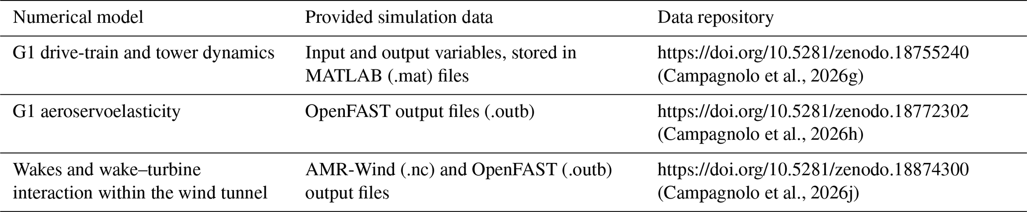
A1 Validation of the synthetic inflow

Figure A1 shows a numerical–experimental comparison of the longitudinal turbulence intensity (TI, lower panels) and the mean longitudinal velocity ${\stackrel{\mathrm{‾}}{u}}_x$ (upper panels), with the latter normalized by the corresponding mean velocity at the Pitot tube position ${\stackrel{\mathrm{‾}}{u}}_{x,\mathrm{P}}$. Figure A1a–d and e–h present the comparison for Mod-TI and High-TI inflow conditions, respectively.

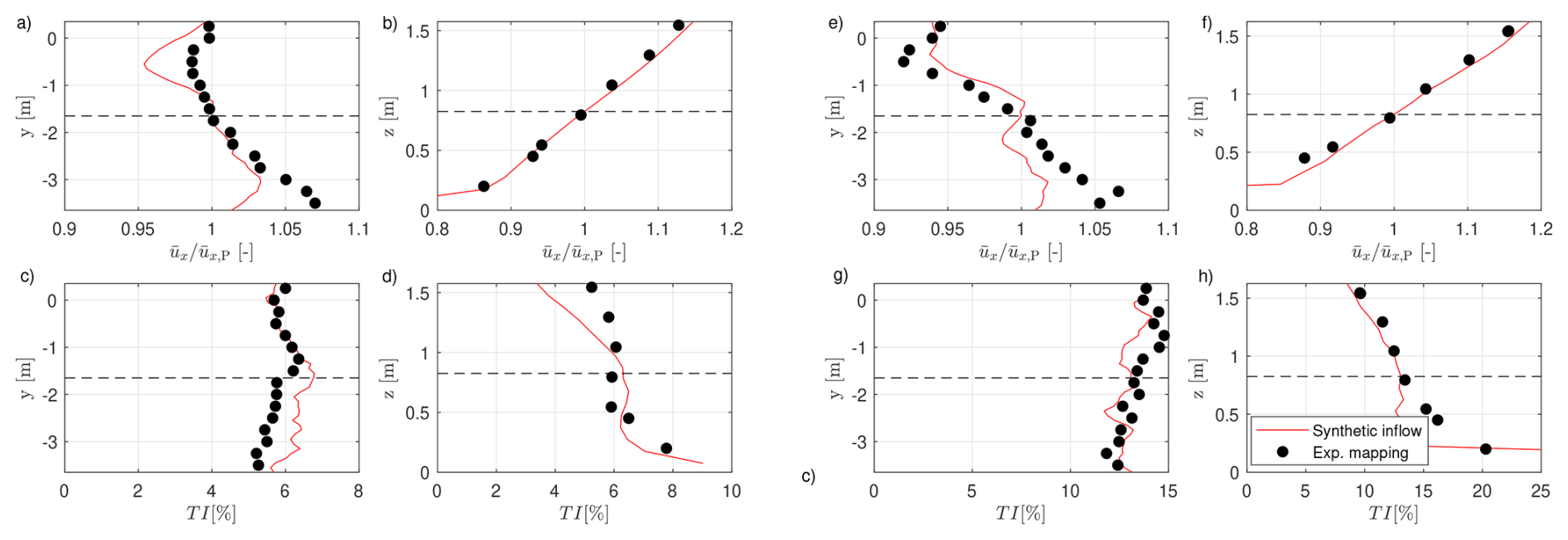
Figure A1 Numerical (red lines) and experimental (black dots) comparison of the longitudinal turbulence intensity (lower panels) and the normalized mean longitudinal velocity (upper panels). Panels (a–d) and (e–h) refer to Mod-TI and High-TI inflow conditions, respectively. The dashed black lines mark the Pitot position.

The synthetic inflow reproduces reasonably well the variability in both the mean velocity and the longitudinal turbulence intensity, along both the lateral direction (Fig. A1a, c, e, and g) and the vertical direction (Fig. A1b, d, f, and h), with errors on the order of a few percentage points. Further comparisons between the turbulent kinetic energy spectra and the autocorrelation of the synthetic inflow and the experimental measurements are reported in Wang et al. (2019).

A2 Validation of the Simulink model

Figure A2 shows a comparison between numerical predictions and experimental data for the most upstream machine in the cluster (WT1), operating under greedy conditions (panels a-d) and under combined yaw misalignment and derating conditions (Fig. A2e–h).

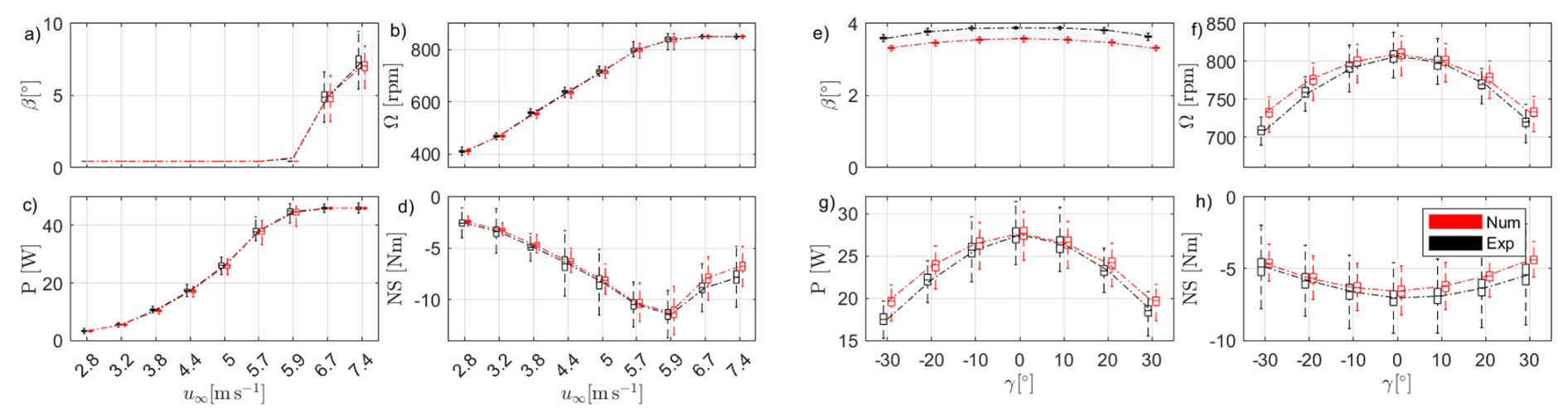
Figure A2 Dataset “Wind turbine data under steady wind direction”. Boxplots (a–d): comparison between experimental (black) data and numerical (red) predictions for greedy operation of WT1 under Mod-TI inflow conditions and varying wind speed (test IDs: [592:6:640]). Boxplots (e–h): comparison between experimental (black) data and numerical (red) predictions for derated (P_d = 0.7) and yaw-misaligned operation of WT1 under Mod-TI below rated inflow conditions (test IDs: [667:673]).

The simulations were performed by reducing the simulated mean wind speed by 0.1 m s⁻¹ relative to the mean of the Pitot measurement. These modest adjustments to the simulated ambient conditions, justified by the uncertainty in wind-speed measurements, improve the agreement with the experimental data. The first 5 s were also discarded to avoid transient effects in subsequent analyses.

Statistical distributions of the considered quantities are represented using boxplots. For each case, the central line of the box indicates the median value, while the box edges correspond to the first and third quartiles. The whiskers extend to 1.96 times the interquartile range, indicating the variability associated with approximately 95 % of the data under the assumption of a normally distributed sample. Outliers are not explicitly shown. The boxplots are positioned and colored to allow direct comparison between experimental and numerical data, as well as between different operating conditions.

The agreement in terms of mean values is very good, except for the blade pitch under combined derating and yaw misalignment. This discrepancy is attributed to the fine-tuning of the optimal pitch implemented in the controller deployed on the G1 turbine (Campagnolo et al., 2023), which differs from the nominal pitch setting implemented in the controller coupled to the simulation environment.

The variability in the considered signals, primarily driven by turbulence in the simulated inflow, is also well captured, except for the tower-base load. This indicates accurate modeling of the drivetrain dynamics in the Simulink environment, whereas the tower motion dynamics is only partially captured by the adopted mass-spring-damper system.

A3 Validation of the OpenFAST model

Figures A3 and A4 compare numerical predictions with experimental data for WT1 under Helix and DY operation, using boxplots. The plots illustrate the sensitivity of the main signals measured on the G1 turbine to variations in the amplitude of the investigated mixing strategy, while the mixing frequency is kept constant.

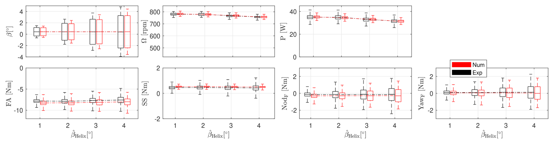
Figure A3 Dataset “Wind turbine data under steady wind direction”. Comparison between experimental (black) data and numerical (red) predictions for CCW Helix operation (f_Helix = 1.075) of WT1 under Mod-TI below rated inflow conditions and varying amplitude ${\widehat{\mathit{\beta }}}_{\text{Helix}}$ (test IDs: [988:991]).

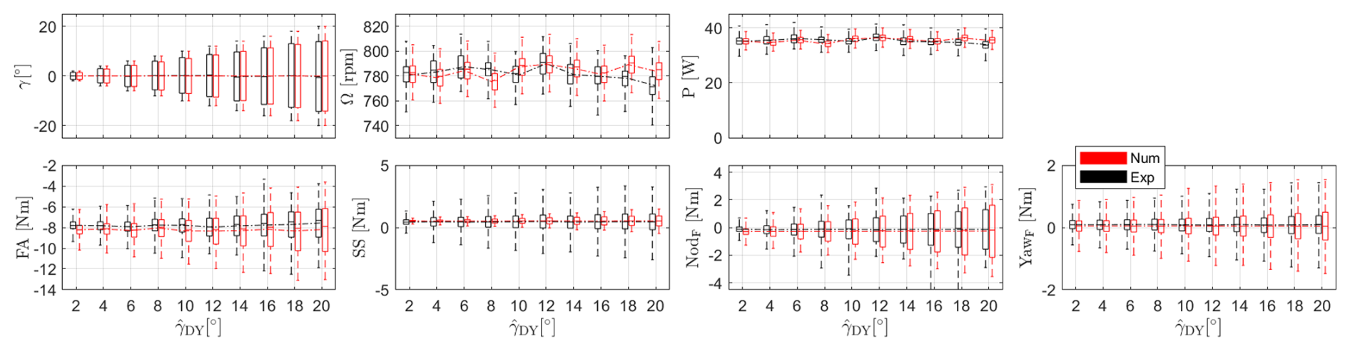
Figure A4 Dataset “Wind turbine data under steady wind direction”. Comparison between experimental (black) data and numerical (red) predictions for DY operation (f_DY = 0.75 Hz) of WT1 under Mod-TI below rated inflow conditions and varying amplitude ${\widehat{\mathit{\gamma }}}_{\text{DY}}$ (test IDs: [1069 1081 1094 1106 1120 1126 1131 1134 1139 1141]).

For the simulations performed with Helix, the simulated mean wind speed was reduced by 0.1 m s⁻¹ with respect to the mean value measured by the Pitot. The simulations were carried out using the ElastoDyn input files for the fast yaw actuator, with the degree of freedom associated with the first blade edgewise mode disabled, as its activation prevented the solver from converging. The first 30 s were also discarded to avoid transient effects in subsequent analyses. Finally, the numerical loads were corrected for the contributions due to the weight of the tower and the rotor–nacelle assembly at zero yaw, as obtained from a no-wind simulation with the rotor at standstill.

The aeroelastic model accurately captures both the mean values and their variability. In particular, the increase in load variability associated with increasing wake-mixing amplitude is reasonably well reproduced. Only the variability in the side–side bending moment at the tower base is underestimated by the model.

The spectrum of the numerical side–side bending moment signal shows a marked underestimation of vibrations at frequencies above the first tower mode. This indicates the need to improve the accuracy of the parameters governing high-frequency tower vibrations, which could be achieved through appropriate tuning based on results from a comprehensive experimental modal analysis of the G1 turbine.

A4 Validation of the AMR-Wind model

Figure A5 shows the average longitudinal velocity field ${\stackrel{\mathrm{‾}}{u}}_x$ predicted by AMR-Wind for two cases of the multiple wake measurement with the lidar dataset (see Sect. 4.1.3): greedy control (Fig. A5a) and yaw misalignment of the two upstream machines (Fig. A5b). The shown data are sampled along a horizontal plane at z = 0.925 m, with the wind speed normalized by ${\stackrel{\mathrm{‾}}{u}}_{x,\mathrm{P}}$, i.e., the average of the numerical wind speed at the Pitot position.

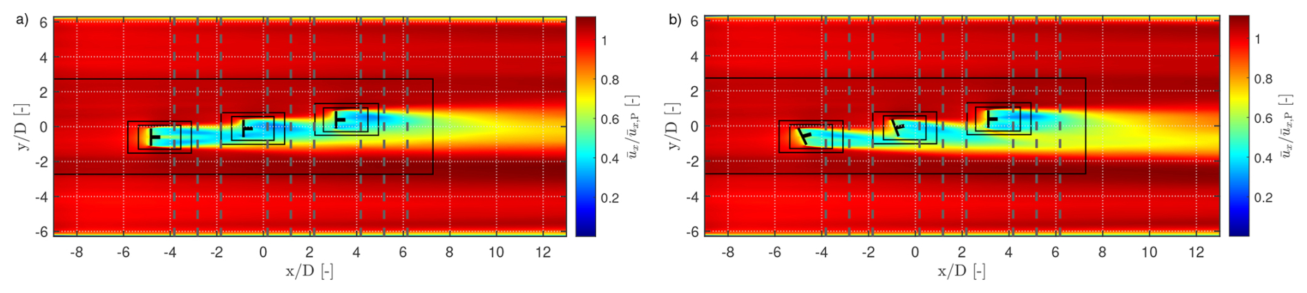
Figure A5 Dataset “Multiple wakes measurement with lidars”. Normalized longitudinal velocity field at z = 0.925 m predicted by AMR-Wind for two cases: greedy control (panel a, ID 1) and yaw misalignment of the two upstream turbines (panel b, ID 4) under Mod-TI below rated inflow conditions. The black rectangles indicate the three AMR levels. The vertical dashed lines mark the streamwise locations where the comparison between lidar measurements and numerical results is performed (see Fig. A6).

The simulations were performed by suppressing all elastic degrees of freedom (DOFs) in OpenFAST to simplify the numerical setup. Furthermore, the first 10 s of simulation data were discarded to remove transient effects.

Figure A6 shows the comparison between the normalized horizontal wake profiles at z = 0.925 m measured experimentally with the lidar (black dots) and predicted by AMR-Wind (red lines). The lidar measurements were first filtered using a simple min–max criterion, removing all velocity samples outside the range 0–8 m s⁻¹. Average velocity-deficit profiles were then obtained by binning the data in the x and y directions with bin sizes of 0.05 and 0.1 m, respectively. The CFD sampling data from AMR-Wind were processed in a similar way. Due to the regular structure of the CFD sampling grid, the data were only binned in the x direction (bin size 0.05 m).

The agreement between numerical and experimental data is very good, with the largest discrepancies observed at 11 D for the case where the two upstream turbines are yaw-misaligned.

Figure A7 shows the comparison between the power gains $P_{\text{Gain}}=P^{\text{WS}}/P^{\text{Greedy}}-\mathrm{1}$ obtained by yaw-misaligning the two upstream turbines relative to the greedy case, as measured experimentally and predicted numerically. The power losses of WT1 induced by the yaw misalignment are well reproduced by the numerical simulations, whereas the power gains of WT2 and WT3 due to wake steering are slightly overestimated. Overall, the wind farm power gain almost falls within the expected uncertainty range of the experimental measurements, estimated by propagating the individual sources of error.

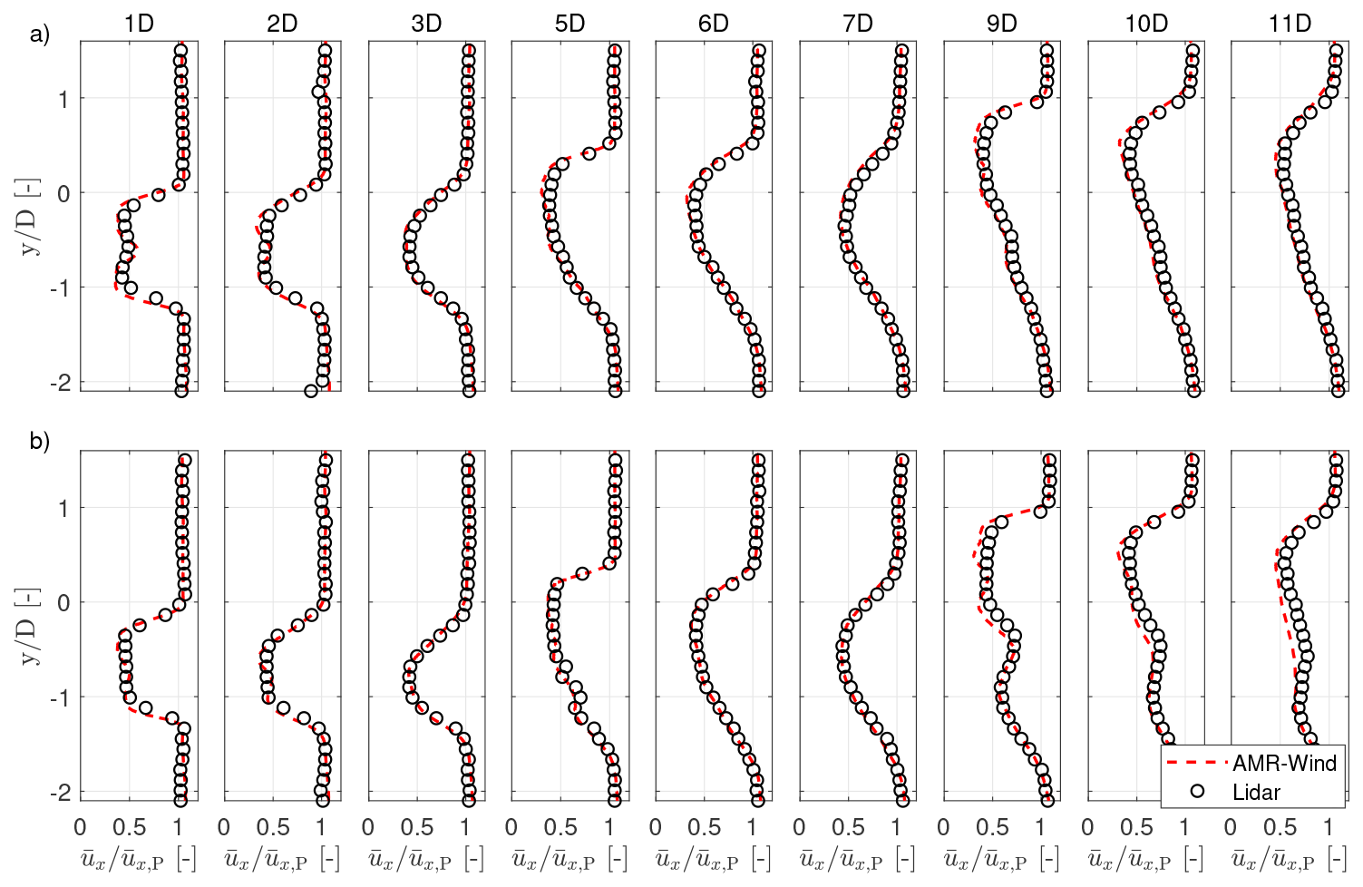
Figure A6 Dataset “Multiple wakes measurement with lidars”. Comparison of experimental lidar data (black dots) and AMR-Wind numerical predictions (red lines) of normalized horizontal wake profiles for greedy control (panel a, ID 1) and yaw misalignment of the two upstream turbines (panel b, ID 4) under Mod-TI below rated inflow conditions. The comparison is performed at several streamwise locations, expressed in rotor diameters downstream of WT1.

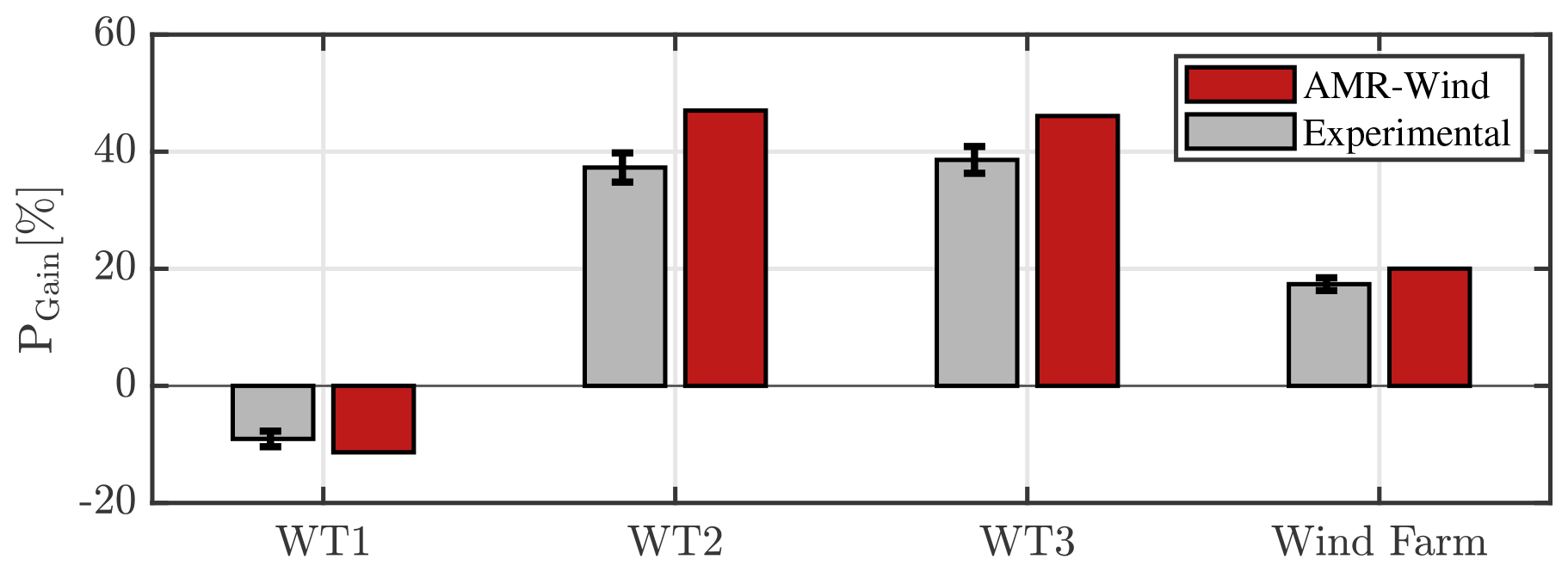
Figure A7 Dataset “Multiple wakes measurement with lidars”. Comparison of experimental measurements and AMR-Wind predictions of the power gain P_Gain relative to greedy control (ID 1), obtained by yaw-misaligning the two upstream turbines (ID 4) under Mod-TI below rated inflow conditions. The error bars represent the uncertainty in the experimental measurements.

Appendix: Nomenclature

A	Rotor swept area [m2]
Cm	Cone coefficient [–]
CP	Power coefficient [–]
CT	Thrust coefficient [–]
D	Rotor diameter [m]
EW	East–west tower-base bending moment [N m]
FA	Fore–aft tower-base bending moment [N m]
f	Frequency [Hz]
fr	Rotor rotational frequency [Hz]
KQ,I	Integral gain of the PI torque controller [N m s]
KQ,P	Proportional gain of the PI torque controller [N m]
Kβ,I	Integral gain of the PI pitch controller [–]
Kβ,P	Proportional gains of the PI pitch controller [s]
Mx,S, My,S	Shaft rotating bending moments [N m]
NodF	Fixed-frame nacelle nodding moment [N m]
NS	North–south tower-base bending moment [N m]
P	Mechanical power [W]
PD	Demanded curtailed power [W]
Pd	Power derating factor [–]
Pn	Normalized mechanical power [–]
PR, QR, ΩR	Rated power [W], torque [N m], and rotor speed [rpm]
rcog	Distance of the rotor–nacelle center of gravity from the tower axis [m]
pdyn	Pitot dynamic pressure [Pa]
Q	Mechanical torque [N m]
R	Rotor radius [m]
SS	Side–side tower-base bending moment [N m]
t	Time [s]
T	Rotor thrust force [N]
u∞	Freestream wind speed [m s−1]
$u_x,u_y,u_z$	Velocity components [m s−1]
vLOS	Line-of-sight velocity measured by lidar [m s−1]
W	Total rotor–nacelle weight [N]
$x,y,z$	Longitudinal, lateral, and vertical coordinates [m]
YawF	Fixed-frame nacelle yawing moment [N m]
zH	Hub height [m]
zSG	Distance between the rotor apex and the tower strain-gauge section [m]

α	Power-law shear exponent [–]
βi	Pitch angle of blade i [°]
δ	Angular resolution (quantization interval) of encoder-based measurements [°]
Δ	Measurement uncertainty at a 95 % confidence level (of the following quantity)
ϵΩ	Rotor speed error [rpm]
γBL	Gearbox mechanical backlash [°]
γ	Yaw misalignment angle [°]
γnac	Nacelle yaw angle [°]
γu	Yaw angle of velocity vector [°]
Φ	Turntable angle [°]
φu	Tilt angle of velocity vector [°]
λ	Tip-speed ratio [–]
ρ	Air density [kg m−3]
σϕ	Standard deviation of wind-direction uncertainty [°]
Ω	Rotor angular velocity [rpm]
ψ	Rotor azimuth angle [°]
(⋅)Dem	Demanded value
(⋅)Meas	Measured value
(⋅)opt	Optimal value
(⋅)P	Pitot probe reference position
(⋅)S	Rotating shaft reference frame
ABL	Atmospheric boundary layer
APC	Active power control
CAD	Computer-aided design
CTA	Constant temperature anemometer
DEL	Damage equivalent load
DIC	Dynamic induction control
DY	Dynamic yaw
IPC	Individual pitch control
LES	Large eddy simulation
PLC	Programmable logic controller
REWS	Rotor effective wind speed
TSR	Tip-speed ratio