Predicting wind turbine aerodynamic loads using laser-scanned blade geometry with validation based on operational and structural data

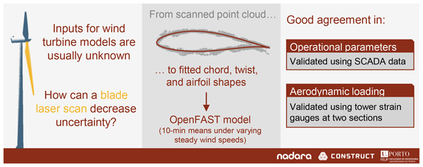
Aeroelastic wind turbine models are key tools in lifetime extension studies, but their application is often hindered by high uncertainty in aerodynamic load predictions. Manufacturers typically do not disclose blade geometry, which drives aerodynamic loading and is therefore an essential input. Furthermore, model outputs are often only compared with supervisory control and data acquisition (SCADA) data, which contain limited information on structural loading. The present work addresses these challenges by using experimental measurements to develop and validate an aeroelastic model of an onshore multi-megawatt wind turbine. Results from the terrestrial laser scanning of a wind turbine blade are processed with a new methodology based on consensus algorithms to derive spanwise chord, twist, and airfoil distributions, which are used as OpenFAST inputs. Simulation results are compared with structural health monitoring measurements of tower bending moments at two elevations, in addition to SCADA data. Moreover, rotor thrust and torque are estimated from the tower measurements and used as additional comparison metrics. The simulations show good agreement with the experimental data, supporting the proposed methodology. A parametric study assesses how the predicted loads are affected by blade geometry, polars, yaw misalignment, and SCADA wind speed uncertainty. The results highlight the usefulness of laser scanning for improving confidence in aerodynamic model inputs, as well as the value of tower load measurements as a complementary validation source to SCADA data. Therefore, the paper proposes and validates a new strategy to obtain a highly reliable model for load estimation, using a quite unique set of diverse measurements and new data processing approaches.

1 Introduction

The demand for renewable energy is increasing, with wind energy already making up a significant share of the global electricity mix and being expected to play an increasingly important role in the coming years (IEA, 2025). In the European Union, for example, there was an installed capacity of onshore and offshore wind energy of 246 GW as of 2025, a number which is expected to grow to 343 GW by 2030 (Costanzo and Brindley, 2026). One hindrance to this projected growth is the number of assets approaching the end of their design life: 65 GW of European wind turbines will be older than the typical design life of 20 years by 2030. This has motivated interest in life extension strategies, which require a more detailed understanding of the behaviour of existing wind turbines to assess their structural integrity for continued operation (Natarajan et al., 2020).

Numerical modelling allows the simulation of wind turbine behaviour under varying operational conditions, providing a foundation for lifetime extension assessments through the estimation of fatigue, which limits turbine lifetime (Burton et al., 2021). While purely data-driven models are gaining popularity (Yang et al., 2021; Wu et al., 2024), physics-based models of varying complexity are widely used for this purpose (Branlard et al., 2024; Zhu et al., 2024; Pimenta et al., 2024). In particular, aeroelastic models are a class of physics-based models which simulate the coupled aerodynamic, structural, and control dynamics of wind turbines. OpenFAST (Jonkman and Buhl, 2005) is one of the most widely used aeroelastic modelling tools in the wind energy community due to its open-source nature and extensive validation history (Guntur et al., 2017; Asmuth et al., 2022; Rinker et al., 2020).

This work focuses on using OpenFAST to assess the quasi-static aerodynamic loads acting on the rotor of a wind turbine. Aerodynamic loading is primarily driven by the blade geometry, control parameters, and environmental conditions. According to a recent report on aeroelastic modelling for life extension (Energy Institute, 2025), these parameters are often difficult to obtain, and the ideal data sources for them are not commonly available in typical engineering scenarios. In particular, environmental characterization should ideally be performed using meteorological mast data measured at multiple heights, with rotor geometry and control parameters provided by the manufacturers. Only a few experimental campaigns in the literature approach these conditions (Boorsma et al., 2023; Schepers et al., 2021; Brown et al., 2024), and they are rarely met in practice. In most cases, blade geometry data are unavailable due to intellectual property protection, while the environmental characterization is based on error-prone nacelle-mounted sensors only. Control parameters are also typically proprietary but can be reasonably estimated using supervisory control and data acquisition (SCADA) data.

The literature reflects the aforementioned difficulties and showcases strategies for their mitigation. Data gaps may be filled using information from reference wind turbine models (Jonkman et al., 2009; Bortolotti et al., 2019). For example, Moynihan et al. (2022) studied the rotor loads of a 2.5 MW turbine using data from a 3 MW reference turbine to fill in missing information, and Pimenta et al. (2020) estimated the structural properties of a 1.8 MW rotor by scaling data from a 5 MW reference model. Another approach is to fit unknown parameters to turbine performance metrics. For example, Wu and Porté-Agel (2012) adjusted the blade chord and twist distributions in order to match a manufacturer thrust curve, while Xie et al. (2025) adjusted the blade twist to match the SCADA-logged power curve. However, there is no guarantee that these approaches yield a physically realistic model, and real measurements of the input data are preferable. Furthermore, the common approach of using only SCADA data for model validation limits the ability to identify the sources of discrepancies between model predictions and real turbine behaviour.

Blade geometry may be directly measured using terrestrial laser scanning (TLS), a technique to assess the geometry of large structures using ground-based lidar technology (Mukupa et al., 2017; Wojtkowska et al., 2021). In the wind energy field, TLS is regarded as a promising technique still requiring widespread validation as a tool to inform wind turbine aeroelastic models (Energy Institute, 2025). A recent work described the application of TLS to reconstruct the outer geometry of a wind turbine blade in a 2 MW turbine (Xie et al., 2025). The authors noted some potential error sources such as wind speed measurement inaccuracies and difficulty in calibrating the twist angle due to lack of a zero reference. TLS has also been applied to measure the deformation of a wind turbine tower (Helming et al., 2021) and to detect defects in wind turbine blades (Stałowska et al., 2025).

The present work combines terrestrial laser-scanning-based blade geometry reconstruction with operational SCADA data and tower-based structural health measurements to develop and validate an aeroelastic model of an onshore multi-megawatt wind turbine. TLS is used to inform the aerodynamic model inputs by reconstructing spanwise chord, twist, and airfoil distributions, including a dedicated alignment procedure to mitigate scan misalignment caused by blade vibrations during data acquisition. Tower bending moments measured at two cross-sections are used as validation metrics, and a method is presented to estimate rotor thrust and torque from these measurements, providing additional validation quantities allowing a more comprehensive structural assessment of the rotor. A parametric study is then conducted to assess the sensitivity of the model to selected uncertainties (blade chord scale, blade twist offset, aerodynamic polar degradation, yaw misalignment, and SCADA wind speed errors) and to evaluate the plausibility of different explanations for observed discrepancies in aerodynamic load predictions.

The remainder of the paper is organized as follows. Section 2 describes the different experimental data sources used, including SCADA data, the structural health monitoring (SHM) system, and the laser scan. Section 3 presents the method used to estimate rotor thrust and torque from the SHM measurements, while Sect. 4 details the process of reconstructing the blade geometry from the laser scan data. The development of the OpenFAST model is described in Sect. 5, while its results and comparison with experimental data are presented in Sect. 6, and the parameter study is shown in Sect. 7. Finally, Sect. 8 summarizes the main conclusions.

2 Data sources

This study was carried out using data from an onshore multi-megawatt wind turbine with a rotor diameter of 80 m. The tower geometry and material properties are known in detail. Regarding blade geometry, only the blade length and the two airfoil families used along the blade are known. Additional parameters given by the manufacturer are the weight and centre of mass location of the nacelle, rotor, and hub, as well as a typical value of the generator efficiency. The additional experimental data supporting the development of the aeroelastic model representing this turbine came from three main sources: firstly, the turbine's SCADA system, which provided the main operational and environmental variables; secondly, a tower SHM system, from which the bending moments were measured at two tower cross-sections; and finally, a laser scan of a blade of a turbine of the same model (with a different tower height), providing a point cloud describing the outer geometry of the blade. The continuous monitoring data (SCADA and SHM) were collected between August and December 2024. This section describes each of these data sources in more detail. Due to confidentiality agreements, the data presented in this paper are anonymized and normalized, thus preserving the general characteristics of the turbine without disclosing specific information.

2.1 SCADA data

As is common practice in the wind industry, the turbine's SCADA system logged data in 10 min statistics consisting of average, minimum, maximum, and standard deviation values. The dataset included operational parameters such as rotor speed, blade pitch angle, electrical power output, and nacelle direction. Additionally, the available environmental parameters included wind speed, wind direction, and ambient temperature. In this work, only the data corresponding to power-producing conditions were considered and were obtained by filtering data points where the 10 min minimum power was positive. Figure 1 shows the main operational variables (generator power P, blade pitch β, and rotor speed Ω) as a function of wind speed, illustrating the turbine's performance characteristics.

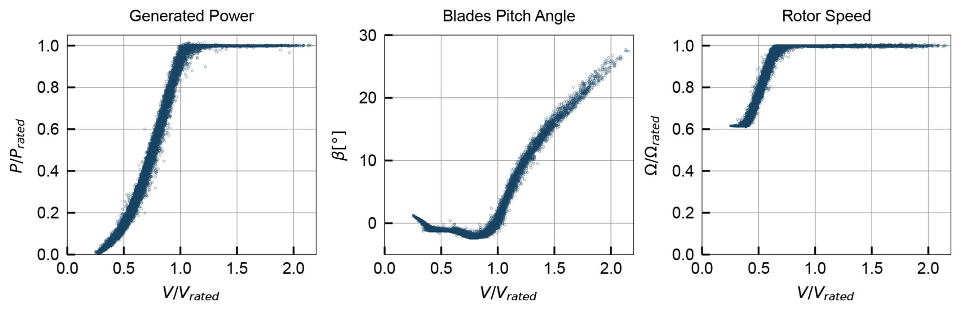
Figure 1 SCADA-logged 10 min averages of power, pitch, and rotor speed as a function of wind speed.

The wind speed logged by the SCADA system corresponds to a measurement from a nacelle-mounted anemometer to which a transfer function is applied in order to estimate the free-stream wind speed at hub height. There were no meteorological masts or lidar systems in the wind farm to provide independent wind speed measurements. These conditions warrant caution when using the SCADA wind speed for comparison with numerical models, as the transfer function may not accurately represent the real wind conditions.

2.2 Laser-scanned point cloud

The terrestrial laser scan was performed while the turbine was parked, with the rotor locked, under low-wind conditions. The scanner was placed at 13 different positions around the turbine, obtaining scans of both the pressure and suction sides of the blade. These scans were aligned into a single reference frame, forming a three-dimensional point cloud. The acquisition primarily targeted one blade (which was oriented vertically and pointing downwards) while also partly capturing the tower, nacelle, hub, and the other two blades. The resulting point cloud is depicted in Fig. 2, in a referential aligned with the tower axis and centred on the tower base, with the studied blade highlighted. Note that, in this figure, the dataset was downsampled to 10 % of the original points for visualization purposes. The blade region contains approximately 5.29×10⁶ points.

Figure 2 Point cloud from the wind turbine laser scan (studied blade highlighted).

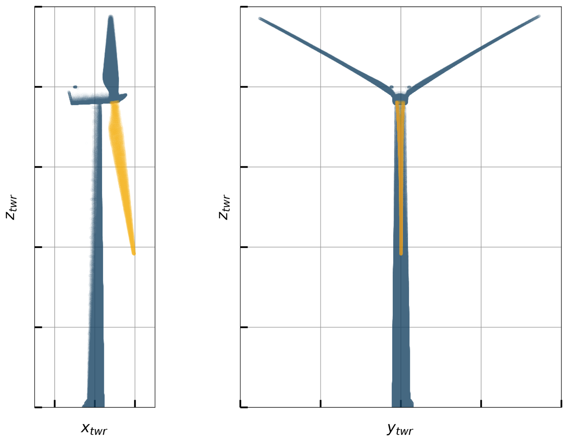
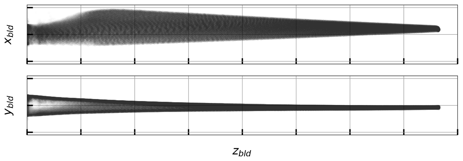
Figure 3 shows the point cloud in the blade region, in a referential aligned with the blade pitch axis and centred on the blade root. The main limitation of this dataset is that some blade vibrations occurred during the measurement due to the low (but non-zero) ambient wind (especially in the flapping direction, corresponding to the y_bld direction). Consequently, the point cloud shows some scatter even after alignment to a consistent reference frame, reflecting the deflections of the blade during the scan. This effect is more pronounced towards the blade tip. This effectively translates to an overestimation of the aerodynamic thickness of outboard blade cross-sections if this effect is not addressed. A strategy to mitigate this effect is presented in Sect. 4.

Figure 3 Point cloud in the scanned blade region.

2.3 SHM bending moments

SHM data were retrieved from the experimental setup depicted in Fig. 4. The instrumentation consists of two tower cross-sections, one near the top (cross-section A) and one near the base (cross-section B). Each cross-section includes four measurement locations (identified with “S”), distributed around the inner circumference of the tower and sampled at 5 Hz. The sensor distribution is shown in Fig. 4 together with the turbine wind rose. At each measurement location, the strain signal is obtained through a bridge circuit. In cross-section A, quarter-bridge configurations are used, with co-located temperature measurements (identified with “T”). In cross-section B, full-bridge configurations are used, consisting of two active and two dummy gauges for temperature compensation.

Figure 4 Experimental setup and characterization of the wind conditions in the wind farm.

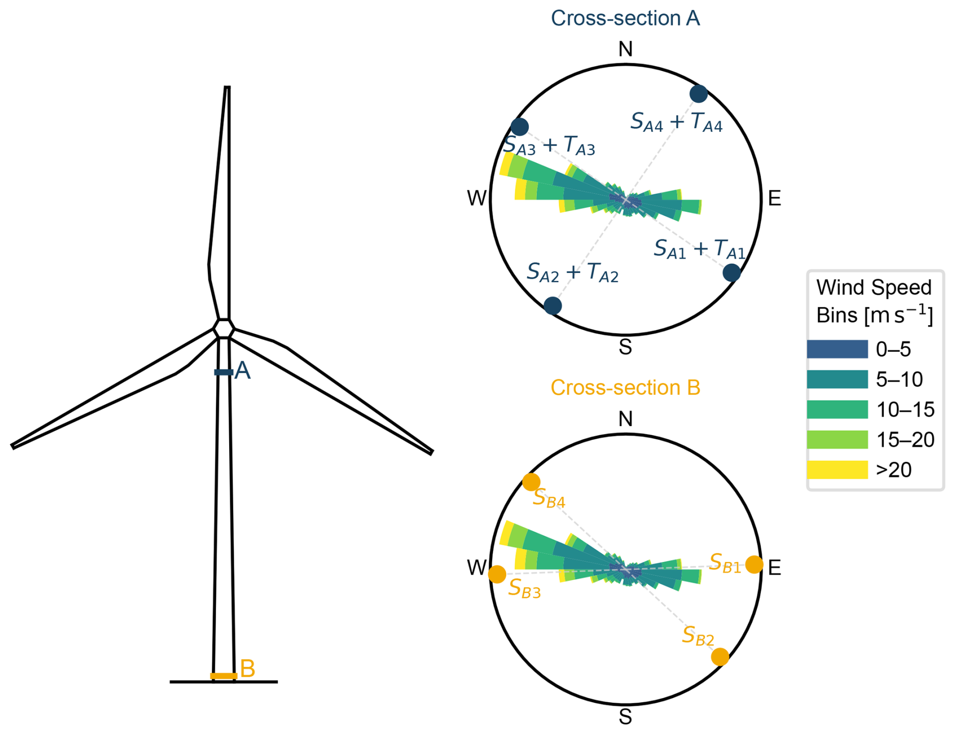
A previous study (Galhardo et al., 2025) used the same instrumentation (but a different monitoring period) to compare different strategies to correct strain gauge drifts and residual thermal effects using measurements during cable untwisting events, when the nacelle rotates 360° to relieve cable torsion. These effects were corrected using the method that led to better results for each cross-section. The corrected stresses were aggregated into 10 min means, and subsequently the bending moments at each cross-section were computed assuming plane stress. Figures 5 and 6 show the bending moments as a function of the SCADA wind speed, in cross-sections A and B, respectively.

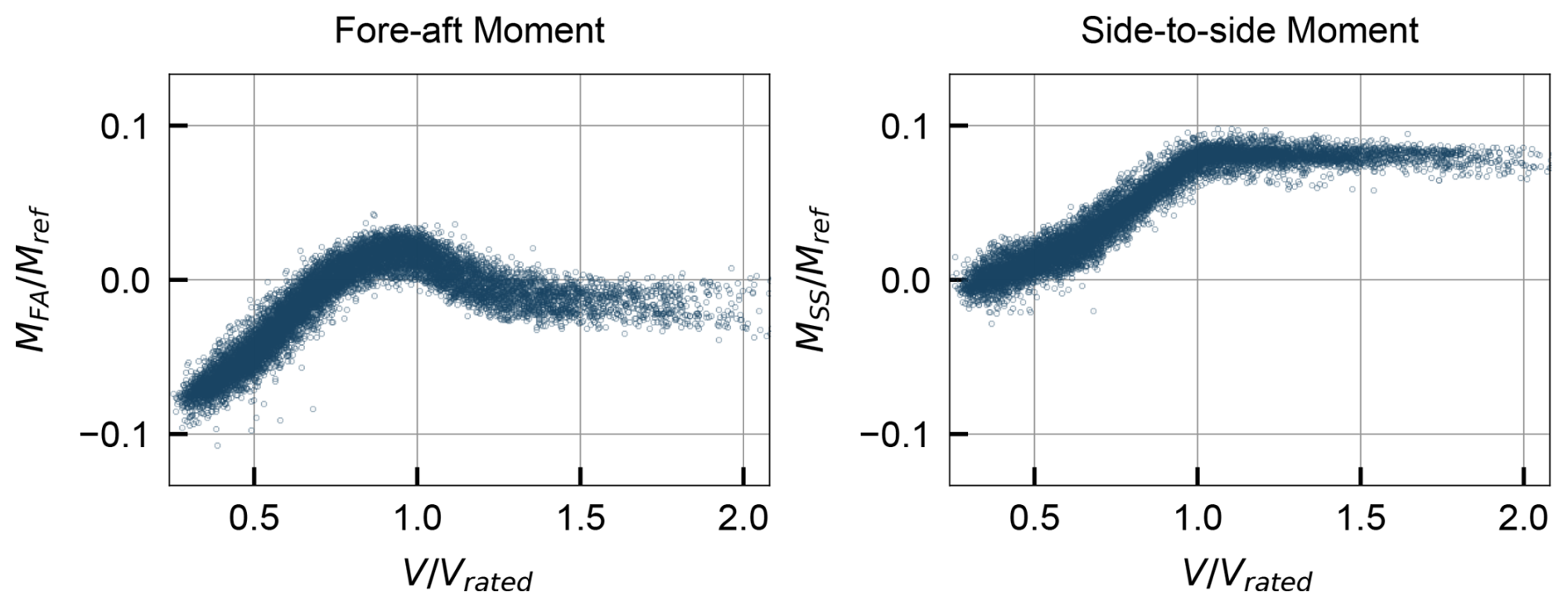
Figure 5 Bending moments (10 min averages) at tower cross-section A as a function of wind speed.

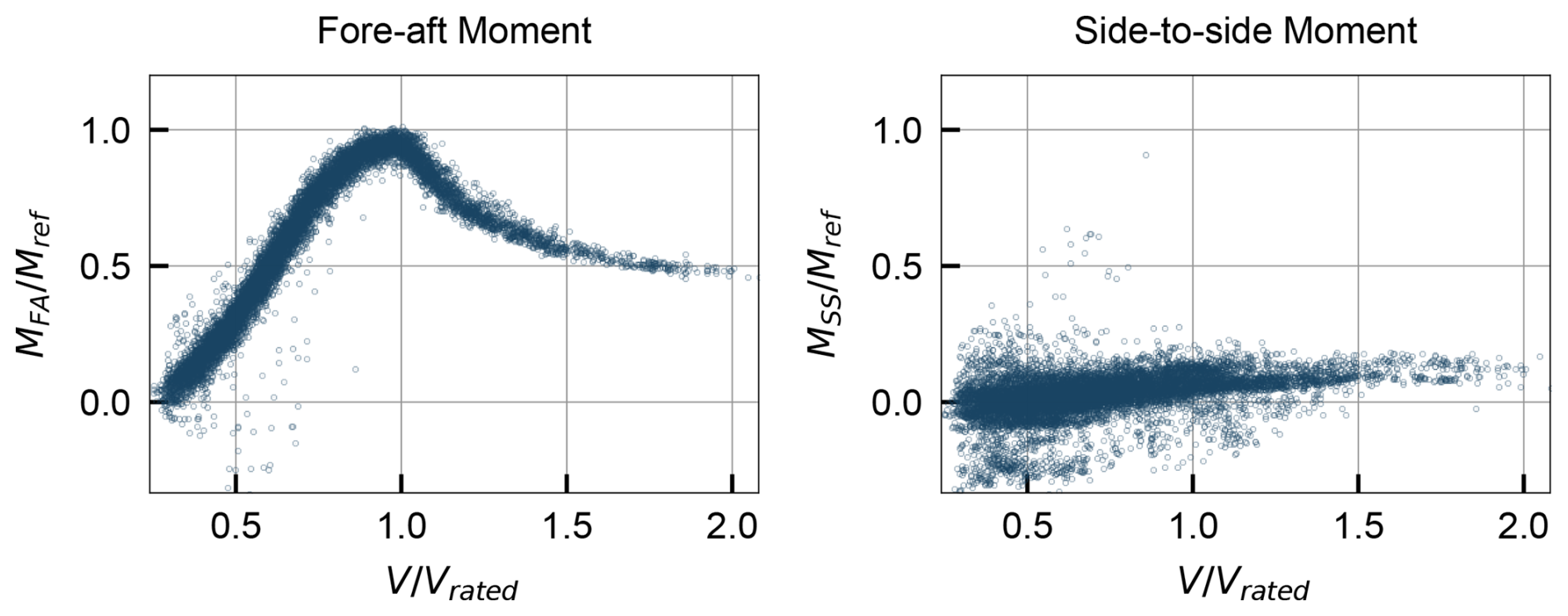
Figure 6 Bending moments (10 min averages) at tower cross-section B as a function of wind speed.

The curves show the typical pattern of increasing bending moments with wind speed until rated power is reached. Beyond rated, the fore–aft moments decrease as pitch control decreases the rotor thrust force, while the side-to-side moments remain roughly constant, as they are dominated by the rotor torque (which is constant for rated power and rotor speed). The scale of bending moments is significantly different between the two cross-sections due to the difference in height. In cross-section A, the fore–aft moment is influenced by the rotor thrust (which has a relatively small lever arm at that height) and the rotor and nacelle overhang moment, while the side-to-side moment is dominated by the rotor torque. In cross-section B, the fore–aft bending moments are much larger, as they are dominated by the lever arm of the rotor thrust, and the side-to-side moments are comparatively small. The scatter in data may be explained by variations in variables such as turbulence intensity or air density, which have a significant effect on the aerodynamic loads. The scatter in M_SS at cross-section B, which is noticeably higher, is also attributed to the sensor layout in relation to the most common wind directions (see Fig. 4), which causes difficulty in accurately resolving the side-to-side bending moment from the strain gauge measurements.

3 Aerodynamic load estimation from tower bending moments

This section describes how the measurements of tower bending moments at two cross-sections are used to estimate the rotor thrust T and torque Q. As illustrated in Fig. 7, the thrust and torque are closely related to the tower-top force and moment in the nacelle-aligned direction, F_x,top and M_x,top. The figure also shows the moments caused by the overhang of the rotor and nacelle assembly in the fore–aft and side-to-side directions, M_overhang,FA and M_overhang,SS, represented in the direction of their effective contribution to the tower-top loads. The shaft tilt θ_shaft is amplified in the figure for visualization purposes.

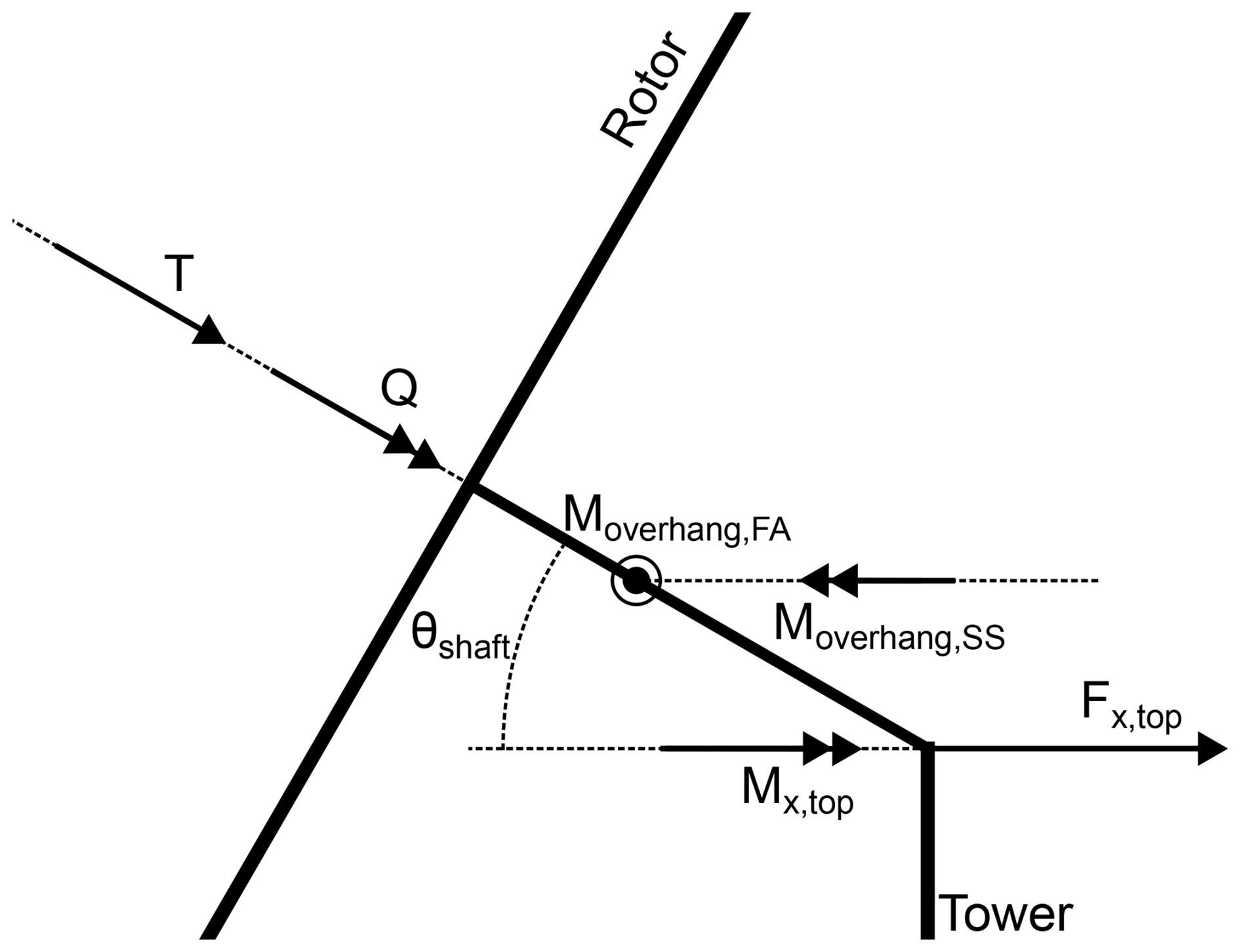
Figure 7 Sketch of the relationship between rotor thrust T and torque Q and the tower-top loads F_x,top and M_x,top.

The tower-top force F_x,top is the projection of the thrust (aligned with the shaft axis) onto the horizontal axis, which is tilted by the angle θ_shaft with respect to the rotor plane. Mathematically, this relationship is expressed as

$$\begin{array}{}\text{(1)}& T={\displaystyle \frac{F_{x,\mathrm{top}}}{\cos \left({\mathit{\theta }}_{\mathrm{shaft}}\right)}}.\end{array}$$

Analogously, the torque Q is related to the tower-top moment M_x,top, considering the shaft tilt angle and also subtracting the side-to-side overhang moment M_overhang,SS:

$$\begin{array}{}\text{(2)}& Q=M_{x,\mathrm{top}}\cos \left({\mathit{\theta }}_{\mathrm{shaft}}\right)-M_{\mathrm{overhang},\mathrm{SS}}.\end{array}$$

The shaft tilt angle θ_shaft is known from the turbine specifications, while M_overhang,SS can be estimated from the known mass and centre-of-mass location of the rotor and nacelle assembly. Therefore, estimating the rotor thrust and torque from the tower bending moments reduces to estimating the tower-top loads F_x,top and M_x,top from the bending moments measured at the two cross-sections.

Figure 8 illustrates the approach taken for the estimation of tower-top loads from the cross-sectional bending moments: we consider a tower of height H and a generic tower cross-section at height z_twr, with local fore–aft and side-to-side bending moments denoted M_FA and M_SS. Assuming the tower behaves as a cantilever beam, the bending moments at the cross-section can be related to the tower-top loads, which can be completely described using two forces F_x,top and F_y,top and two bending moments M_x,top and M_y,top (the latter being influenced by the shear in the rotor wind field).

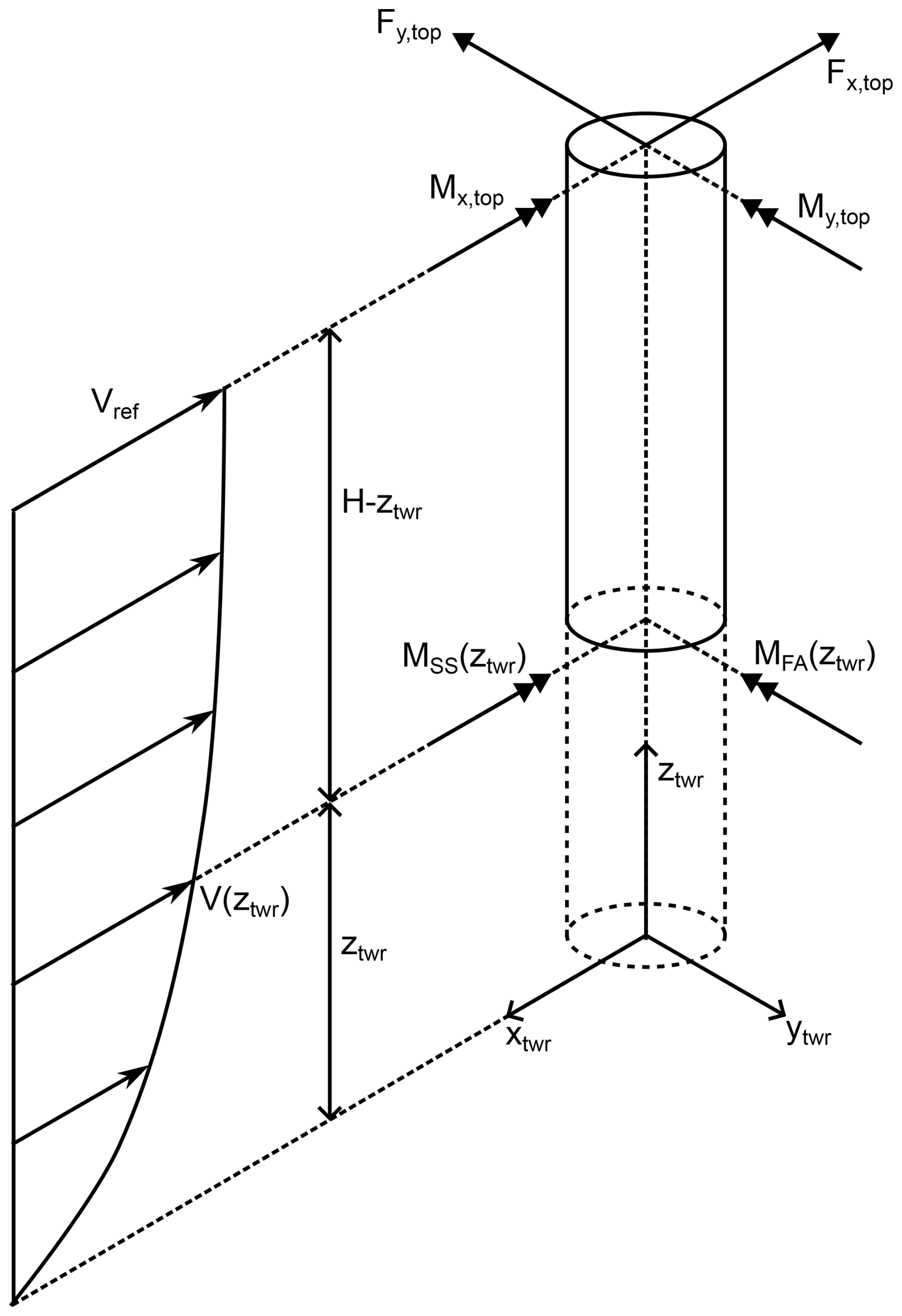
Figure 8 Sketch of the tower loads considered in the load estimation and definition of adopted notation for forces and bending moments.

The wind speed profile along the tower height $V_{z_{\mathrm{twr}}}$ is also considered and is assumed to follow a power law with shear coefficient α_shear and tower-top height reference wind speed V_ref:

$$\begin{array}{}\text{(3)}& V\left(z_{\mathrm{twr}}\right)=V_{\mathrm{ref}}{\left({\displaystyle \frac{z_{\mathrm{twr}}}{H}}\right)}^{{\mathit{\alpha }}_{\mathrm{shear}}}.\end{array}$$

The local bending moments are assumed to follow the relationship in Eq. (4), which considers the contributions of the tower-top forces and moments, as well as the contribution of the wind-induced tower drag on the tower itself. The tower drag is modelled as a distributed load with a constant drag coefficient C_d and a diameter profile D(z) along the tower height.

$$\begin{array}{}\text{(4)}& \left\{\begin{array}{l}{M}_{\mathrm{FA}}\left(z_{\mathrm{twr}}\right)=(H-z_{\mathrm{twr}})F_{x,\mathrm{top}}+M_{y,\mathrm{top}}\\ +\underset{z_{\mathrm{twr}}}{\overset{H}{\int }}{C}_{\mathrm{d}}\frac{\mathrm{1}}{\mathrm{2}}\mathit{\rho }\left(V\right(z_{\mathrm{twr}}\left){)}^{\mathrm{2}}\mathrm{D}\right(z)z\mathrm{d}z\\ M_{\mathrm{SS}}\left(z_{\mathrm{twr}}\right)=-(H-z_{\mathrm{twr}})F_{y,\mathrm{top}}+M_{x,\mathrm{top}}\end{array}\right.\end{array}$$

In this work, the two instrumented tower cross-sections yield measurements of the bending moments in the fore–aft and side-to-side directions M_FA and M_SS at two tower heights z_A and z_B. Estimating the tower drag with parameters C_d=0.5 and α_shear=0.2, this system has four unknowns: the tower-top forces F_x,top and F_y,top and moments M_x,top and M_y,top. Using the measured bending moments at the two cross-sections, Eq. (4) can be written twice for two values of z_twr, yielding a system of four equations with four unknowns, which can be solved to estimate the tower-top loads. It should be noted that the drag contribution is small compared to the tower-top loads, having negligible values except for very high wind speeds, so the selected parameters for drag characterization do not significantly affect the load estimates.

In summary, the method presented in this section yields estimates of the rotor thrust and torque from the tower bending moments measured at two cross-sections. Inverting Eq. (4) allows the estimation of the tower-top loads, which are then related to the rotor thrust and torque using Eqs. (1) and (2). Figure 9 shows the estimated rotor loads as a function of wind speed, using the tower bending moments presented in Sect. 2.3.

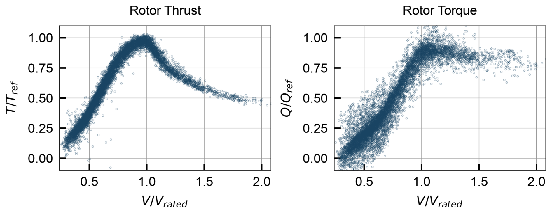
Figure 9 Estimated rotor loads at hub height (10 min averages) based on the tower bending moments in cross-sections A and B.

The curves exhibit the expected patterns: thrust increases with wind speed until rated power is reached, then decreases as pitch control reduces rotor thrust. Torque increases similarly until rated power, where it remains constant. The scatter in the torque curve is higher, which is explained by the higher scatter in the side-to-side bending moments at tower section B, as discussed in Sect. 2.3.

4 Blade geometry reconstruction from laser scan

This section describes the processing steps applied to the laser scan point cloud to extract estimates of the chord, twist, and airfoil shapes along the blade span. The main challenge is to mitigate the effect of blade vibrations during the scan, which caused the different scans to show some misalignment among each other, with a magnitude that increases towards the blade tip. The procedure described below was applied at 39 discrete spanwise stations defined at 1 m intervals along the blade. For a given station nominally located at z^*, the corresponding cross-section was defined as the set of points satisfying $|z_{\mathrm{bld}}-z^{*}|<\mathrm{0.2}\mathrm{m}$. For each station, the points were treated two-dimensionally in the local cross-section plane defined by the x_bld and y_bld axes.

Figure 10 shows the point cloud at two representative blade cross-sections (at $z_{\mathrm{bld}}/R=\mathrm{0.25}$ and $z_{\mathrm{bld}}/R=\mathrm{0.75}$, with R being the rotor radius), where different colours represent different scans. The scatter in the points is evident, especially at the outer section. To address this, an iterative alignment procedure was implemented as follows.

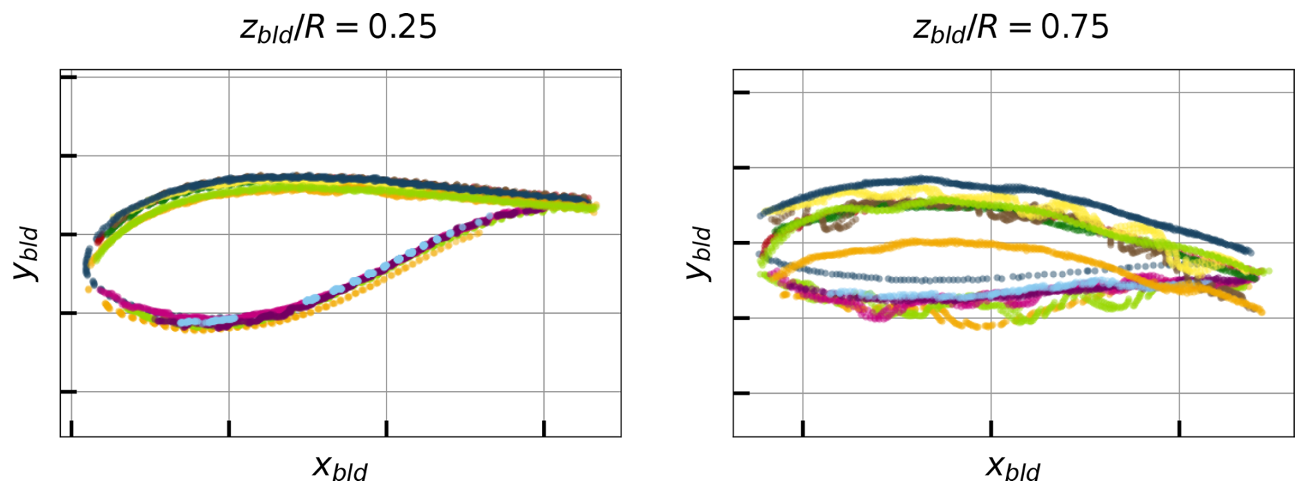
Figure 10 Point cloud at two blade cross-sections (different colours represent different scans).

4.1 Consensus-based scan alignment

A visual inspection of the different scans revealed that individual scans predominantly covered either the low-pressure (LP) side or the high-pressure (HP) side of the blade. The scans were manually classified accordingly and processed separately for each blade side. For each side, the scatter due to blade vibrations was mitigated using a consensus-based alignment procedure described here. In this context, the alignment can be interpreted as estimating, for each scan, a rigid in-plane translation that minimizes the distances between the scan points and a common reference curve (the consensus), based on nearest-neighbour correspondences.

An initial smooth consensus curve was first fitted to the points. Each individual scan cross-section was then aligned to this consensus by estimating a rigid translation in the cross-section plane, computed by minimizing distances to nearest-neighbour correspondences with the consensus curve. After translating all scans, the consensus curve was refitted to the aligned data. This align-refit procedure was repeated iteratively until the consensus curve stabilized. The resulting consensus curves were not used directly as final geometric representations, but only as intermediate constructs to achieve consistent alignment of the individual scans. Figure 11 illustrates the aligned cross-section point clouds for a representative spanwise station, highlighting the substantial reduction in scatter achieved through the alignment process in comparison with the data in Fig. 10.

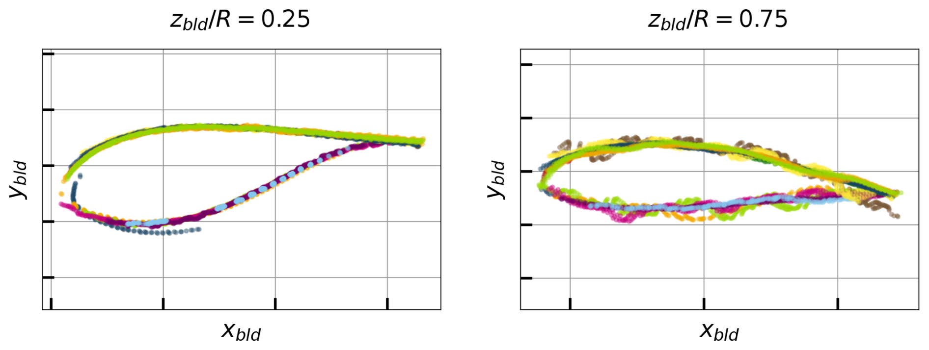
Figure 11 Point cloud at two blade sections after alignment (different colours represent different scans).

4.2 Airfoil shape fitting

Following the consensus-based alignment, each of the selected 39 spanwise stations is represented by an aligned two-dimensional point cloud describing the local blade cross-section. At this stage, points from all retained scans were pooled together, yielding a single aggregated representation of the section geometry. The next step was to fit an airfoil shape to the aligned point cloud.

To constrain the fitted shapes to physically realistic profiles and to improve computational efficiency, a predefined database of candidate airfoils was defined, based on two airfoil families which were specified by the manufacturer (also including circular airfoils and mixtures of circular airfoils with the specified families to better capture the region near the root). Each airfoil geometry was stored in normalized form (unit chord with the leading edge at the origin) and discretized using 200 points along the contour. These candidate airfoils are expected to cover the range of airfoil shapes used along the blade span.

For each spanwise station, every candidate airfoil in the database was evaluated independently. The evaluation consisted of fitting the candidate airfoil to the section's point cloud through a transformation with four parameters: a scale factor c, an in-plane rotation angle α_x, and translations t_x and t_y in the x_bld and y_bld directions, respectively. This transformation and its parameters are depicted in Fig. 12. For each candidate airfoil, the transformation parameters were adjusted to minimize a fitting error between the transformed airfoil contour and the measured point cloud. The best-fitting airfoil was then selected based on the lowest fitting error. This procedure was repeated for all spanwise stations.

Figure 12 Airfoil fitting transformation parameters.

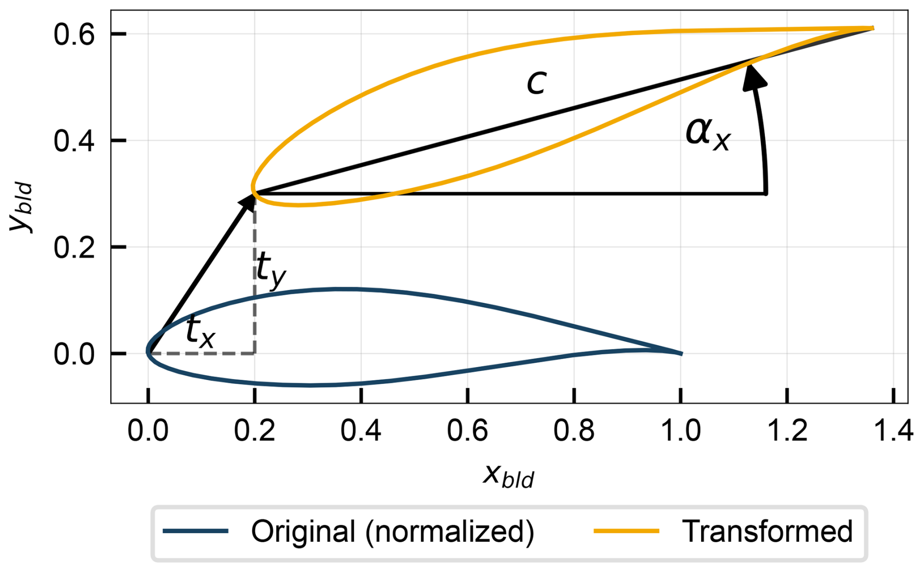
The optimal set of parameters fitting each candidate airfoil shape to each spanwise station's point cloud was obtained by minimizing a nearest-neighbour distance measure between them. For each measured point, the Euclidean distance to the closest vertex of the discretized airfoil contour was computed. A Huber loss function (Huber, 1964) was applied to the resulting distance vector to reduce sensitivity to outliers and poorly resolved regions, and the mean Huber loss was used as the objective function. The resulting bounded nonlinear optimization problem was solved with respect to the four transformation parameters using the gradient-based optimization algorithm L-BFGS-B (Zhu et al., 1997). The process was stopped automatically when further parameter updates produced no meaningful reduction in the fitting error or when the estimated local slope of the objective indicated that a minimum had been reached.

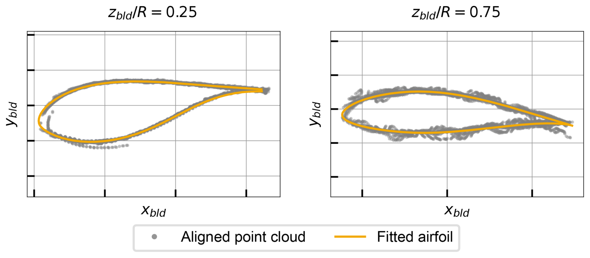
Thus, this procedure selected the best-fitting airfoil shape from the database for each spanwise station and provided an estimate of each station's scale, orientation, and position. Examples of fitted airfoil shapes at two representative blade sections are compared with the aligned point cloud in Fig. 13.

Figure 13 Fitted airfoil shapes at two blade sections.

4.3 Estimation of aerodynamic parameters

Finally, the fitting results are related to the aerodynamic parameters which need to be input in the aeroelastic models. Firstly, the fitted scale parameter directly provides a local chord estimate. In addition, translation parameters t_x and t_y yield an estimate of the aerodynamic centre (assumed to be at 25 % of the chord), which can be used to derive spanwise trends in the section reference line (blade curvature and sweep). Finally, although the rotation angle α_x is evidently related to the local twist angle, the twist definition requires some care. It is necessary to ensure that the zero-twist reference is consistent with that used in numerical models, as even small twist offsets cause significant changes in performance (Xie et al., 2025). The twist angle is defined as the angle between the chord line and the rotor plane. Since the laser scan includes points in the nacelle and tower, the twist can be rigorously determined as depicted in Fig. 14.

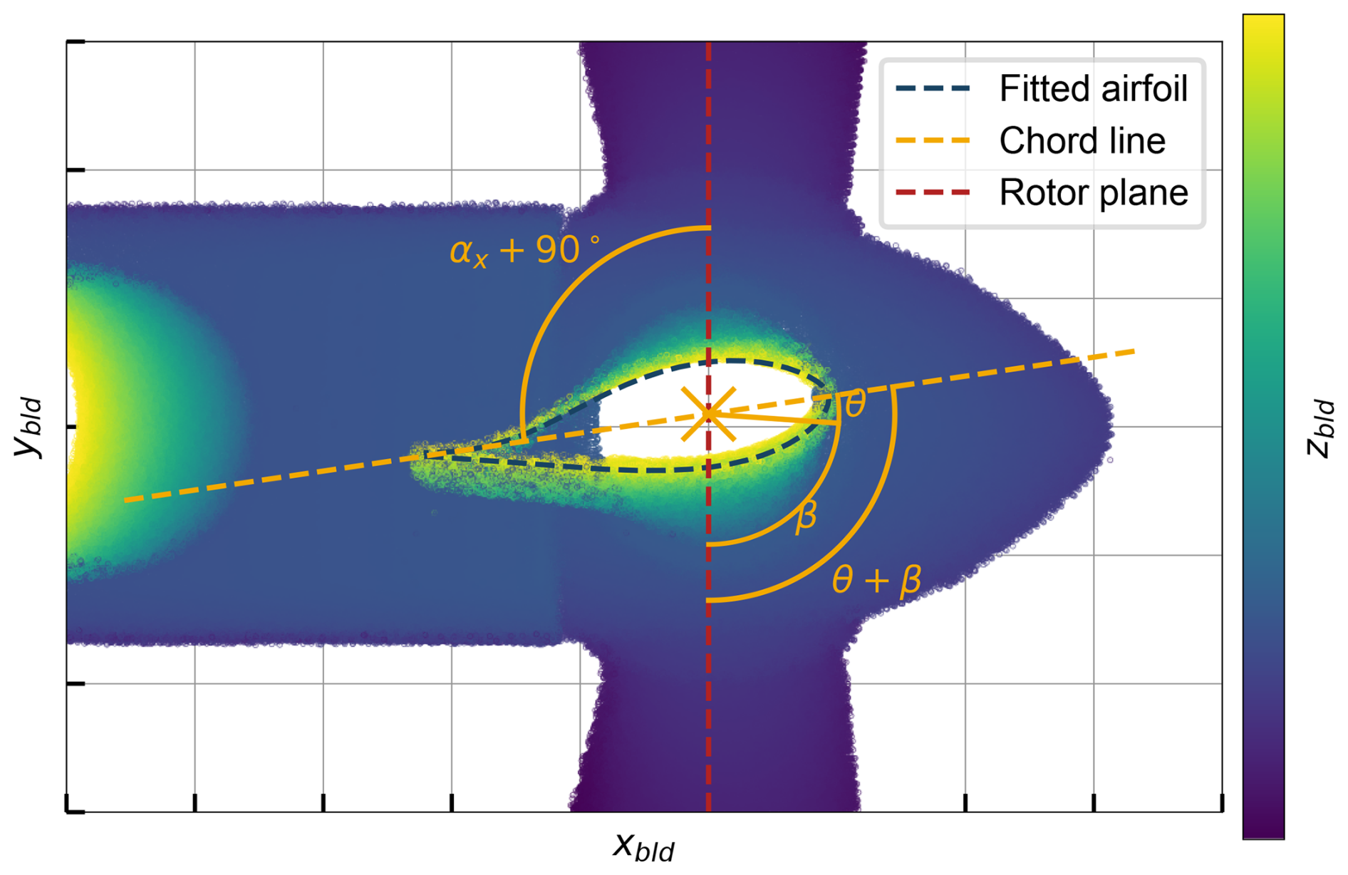
Figure 14 Determination of airfoil twist (example using a clipped point cloud view, showing all points with $z_{\mathrm{bld}}/R<\mathrm{0.25}$), looking from the ground in a referential aligned with the blade pitch axis.

The figure depicts a clipped view of the point cloud, in the referential aligned with the blade axis, showing all points with $z_{\mathrm{bld}}/R<\mathrm{0.25}$. Since the laser scan includes points in the nacelle and tower, the definition of the rotor plane is non-ambiguous. The figure also shows the fitted airfoil at the $z_{\mathrm{bld}}/R=\mathrm{0.25}$ station, along with its chord line. The angle between the chord line and the rotor plane is the sum of the local twist angle at that station θ(z_bld) with the blade pitch angle β. The figure also shows that θ(z_bld)+β is equal to α_x(z_bld)+90°. This yields the following expression for the local twist angle:

$$\begin{array}{}\text{(5)}& \mathit{\theta }\left(z_{\mathrm{bld}}\right)={\mathit{\alpha }}_x\left(z_{\mathrm{bld}}\right)+\mathrm{90}\mathit{°}-\mathit{\beta }.\end{array}$$

With α_x(z_bld) obtained from the airfoil fitting procedure and β known from the SCADA data at the time of the scan, this expression allows the calculation of the twist distribution along the blade span with a zero-twist reference consistent with that used in numerical models.

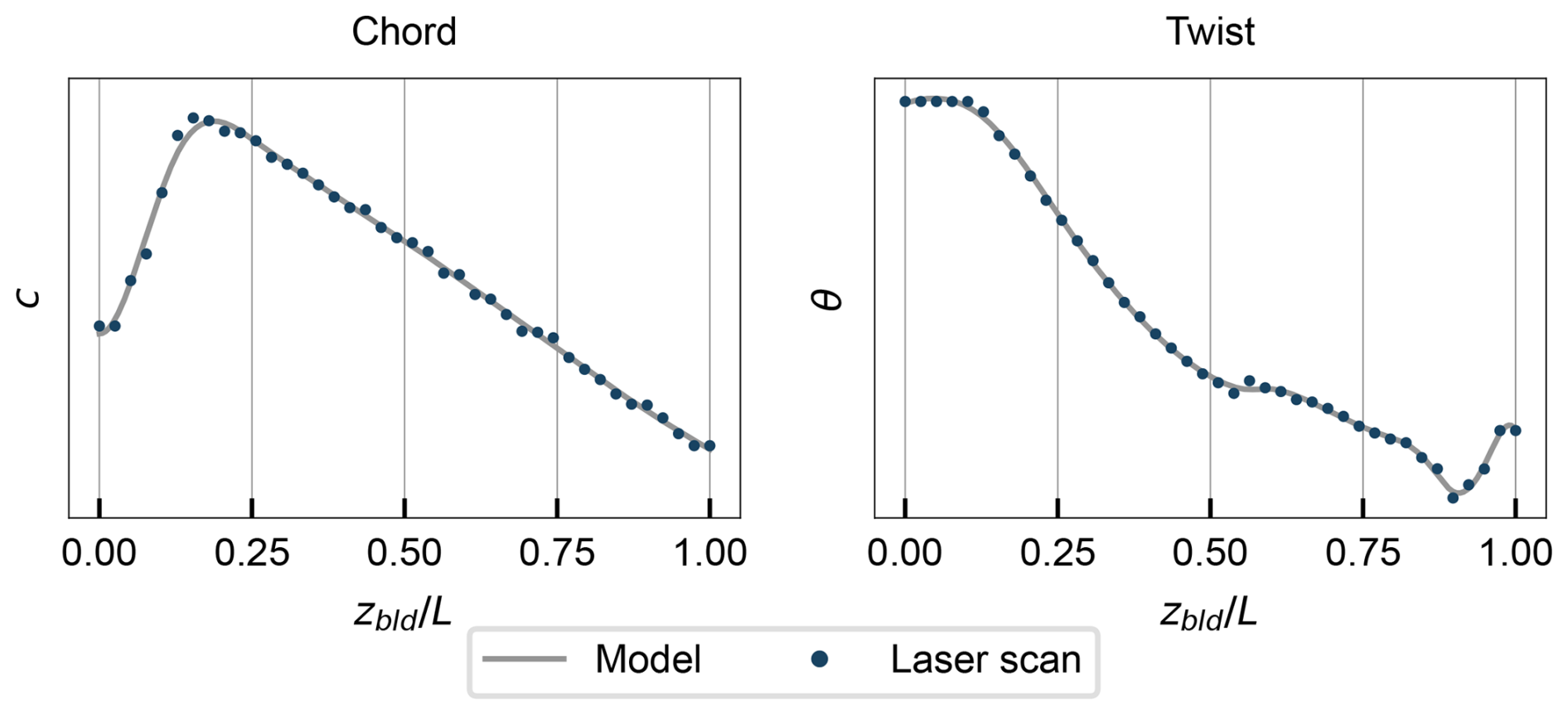
Chord and twist distributions used in the numerical models were derived from the laser scan, where the estimates at discrete spanwise stations were smoothed to reduce the effect of fitting noise. Figure 15 compares the final chord and twist distributions with the laser scan estimates.

Figure 15 Blade chord and twist distributions input to aeroelastic models.

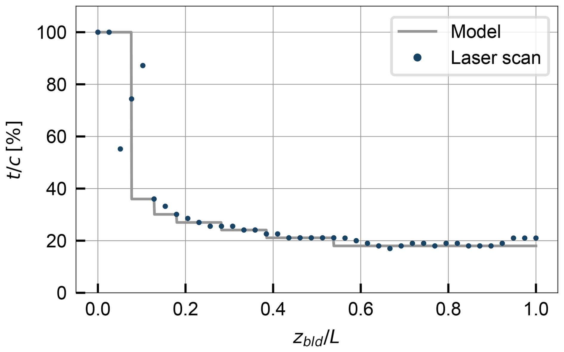
The determination of the spanwise airfoil shapes required a more manual approach based on the fitted airfoils and engineering judgement. Apparent thickness fluctuations between adjacent stations were treated as scan-induced noise; therefore, contiguous regions were constrained to share a single airfoil shape and to follow a monotonic thickness reduction toward the tip. The resulting spanwise distribution of airfoil thickness is shown in Fig. 16, where regions of constant thickness correspond to regions with the same airfoil type. The high variations near the root reflect the difficulty of fitting the airfoil shape in that region, where the blade geometry is more complex and does not follow typical aerodynamic shapes. However, this region's contribution to the overall aerodynamic performance is small and is not expected to affect the results.

Figure 16 Airfoil aerodynamic thickness distribution.

5 Baseline numerical model

A numerical model of the turbine was developed using the aeroelastic code OpenFAST v4.0.0 (Jonkman et al., 2024), which is described in this section. A short overview of the modelling approach is presented here, focusing on the most relevant aspects for this work, with more details available in the software user guide (Jonkman and Buhl, 2005).

5.1 Aerodynamic modelling

The interaction of the wind with the turbine is calculated in the AeroDyn module, which employs the blade element momentum (BEM) theory (Burton et al., 2021), with additions and corrections for effects such as tower shadow, tip losses, and hub losses. The blades are discretized into a finite number of nodes, where the chord, twist, curvature, and sweep are specified. Each section is associated with an airfoil, for which the lift and drag coefficients as a function of angle of attack are provided as input. The tower drag is modelled with a constant drag coefficient of C_d=0.5. The lift and drag forces are calculated at each blade element based on the local relative velocity and user-specified airfoil polars. These forces are then integrated along the blade span to obtain the aerodynamic loads, which are passed to the structural module for load and response calculations.

The airfoil polars were generated using XFOIL (Drela, 1989) and the usual corrections and extrapolations. For each airfoil shape used in the model, the local Reynolds number was determined based on the average chord length, the inflow velocity (calculated from the rated wind speed and rotor speed, assuming an axial induction factor of $\mathrm{1}/\mathrm{3}$), and the kinematic viscosity of air at 15 °C. The corresponding Mach number was also computed, using the local inflow speed and the speed of sound at 15 °C. XFOIL was then used to compute the polars over a range of angles of attack from −20 to 20°, with transition to turbulence forced at 10 % of the chord to reflect the typically high surface roughness of wind turbine blades. As XFOIL provides polars for two-dimensional flow, three-dimensional corrections were subsequently applied: the Du-Selig method for lift (Du and Selig, 1998) and the Eggers method for drag (Eggers et al., 2003). Finally, the polars were extrapolated to cover the full angle of attack range (−180 to 180°) using the Viterna method (Viterna and Corrigan, 1981). These steps were automated using the openfast-toolbox package (NREL, 2025).

5.2 Structural modelling

The structural response to the applied loads is calculated with the ElastoDyn module, which employs a combined modal and multi-body formulation. The modal formulation is used to model both the tower and the three blades, allowing for the calculation of loads and displacements as a function of time. The key inputs are the mass and stiffness distributions of the components, as well as the mode shapes of the considered modes (two fore–aft and side-to-side modes for the tower and two flapwise and one edgewise modes for each blade). The nacelle and hub are modelled as rigid bodies.

The tower mass and stiffness distributions were calculated based on the tower geometry provided by the manufacturer. The equivalent information was not available for the blades, so the blade mass and stiffness distributions were scaled from the IEA 3.4 MW reference turbine (Bortolotti et al., 2019). The mass distribution scaling was performed knowing the total blade mass, while the stiffness distribution scaling was performed to preserve the ratio of stiffness to mass along the span. Since this work focuses on the 10 min means of loads and performance, and dynamic structural response is not studied, the structural properties of the blades have a negligible impact on results, and the scaling approach is justified.

The drivetrain is modelled as a torsional spring whose parameters were directly copied from the IEA 3.4 MW reference turbine. The gearbox efficiency was calculated based on the SHM-measured aerodynamic power (calculated from the SHM-measured rotor torque and the SCADA-measured rotor speed) in comparison with the generator power.

5.3 Control system modelling

Although the details of the controller are proprietary and were not provided by the manufacturer, SCADA data allow for a satisfactory characterization of the controller behaviour. The controller was modelled using ROSCO (Abbas et al., 2024), an open-source wind turbine controller modelling tool developed by NREL. For a clearer controller characterization according to the logic inherent to ROSCO, the tip speed ratio (TSR) λ and the generator torque Q_G are now introduced through Eqs. (6) and (7) (where η_G is the generator efficiency, obtained from manufacturer data sheets).

$$\begin{array}{}\text{(6)}& {\displaystyle }\mathit{\lambda }={\displaystyle \frac{\mathrm{\Omega }R}{V}}\text{(7)}& {\displaystyle }{Q}_{\mathrm{G}}={\displaystyle \frac{P}{\mathrm{\Omega }{\mathit{\eta }}_{\mathrm{G}}}}\end{array}$$

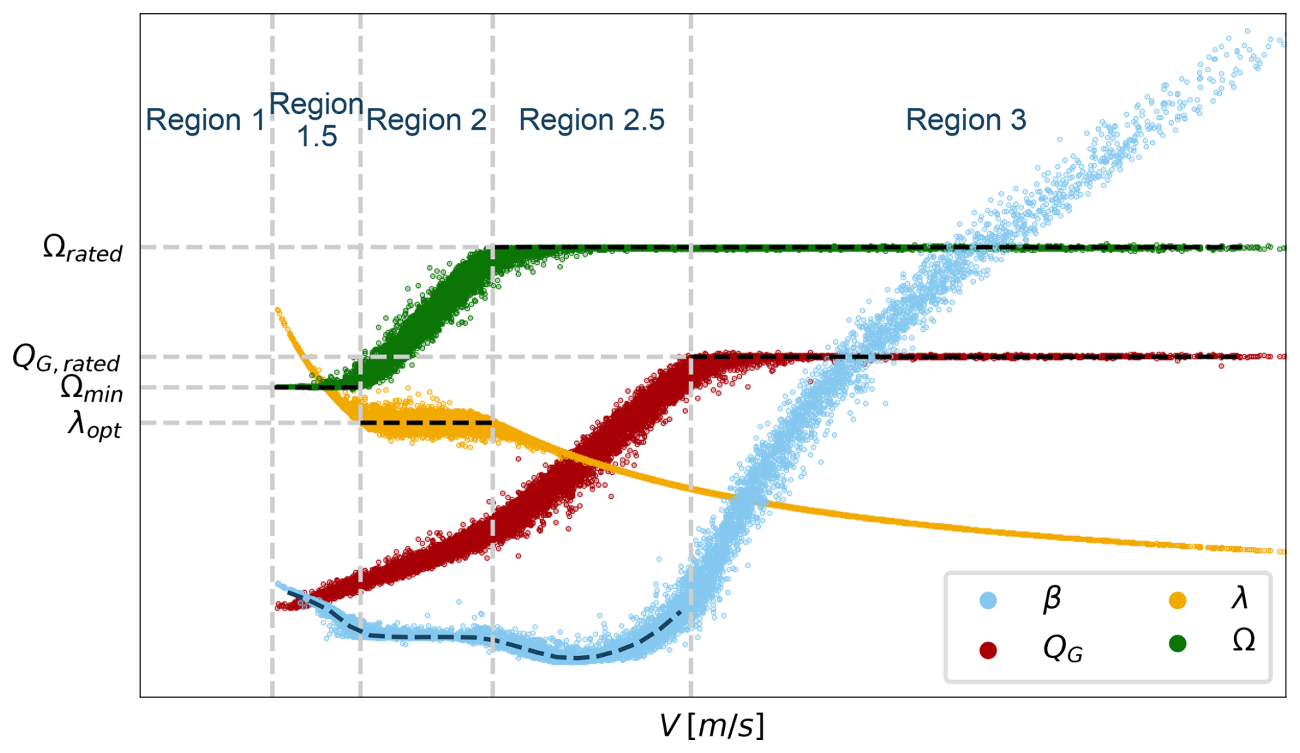
Figure 17 Controller characterization obtained from 10 min averaged SCADA data, with the dashed black lines denoting controller set points (different vertical scale for each variable).

The characterization of the controller set points defined in the numerical model and their inference from SCADA data are summarized in Fig. 17, which shows scatterplots of pitch, generator torque, TSR, and rotor speed versus wind speed, as well as the set points in dashed black lines and the regions of operation according to the nomenclature used by Abbas et al. (2022).

The different regions are numbered in increasing order of wind speed and are modelled with different control strategies, which are now described. Region 1 corresponds to wind speeds below cut-in, where the turbine is not in operation. In regions 1.5, 2, and 2.5, the pitch angle follows a look-up table as a function of wind speed, while the generator torque is the controlled variable. The torque controller aims to maintain rotor speed at its minimum and maximum values Ω_min and Ω_max in regions 1.5 and 2.5, respectively. In region 2, it aims to keep TSR constant at an optimal value λ_opt that maximizes power production. In region 3, the generator torque is constant and equal to its rated value Q_G,rated, while the pitch angle is the controlled variable. Since the rotor speed is also constant and equal to its rated value, this translates to constant rated power.

6 Comparison of baseline model results with experimental data

This section presents the results of simulations with the aeroelastic model described in Sect. 5 and compares them against experimental data. Section 6.1 compares simulated operational data with the SCADA measurements, Sect. 6.2 compares simulated tower loads with the SHM measurements, and Sect. 6.3 compares the simulated rotor thrust and torque with the estimates obtained from tower bending moments. These comparisons are all performed using results from steady-wind simulations, while the effect of turbulence is studied separately in Sect. 6.4.

The steady-wind results were obtained by performing simulations with hub height wind speeds ranging from the cut-in wind speed to the cut-out wind speed, in increments of 1 m s⁻¹. The wind profile followed a power law with a shear coefficient α_shear=0.2, and the air density was set to 1.225 kg m⁻³. Each simulation was run for 200 s to allow convergence, and the last 50 s was used to compute mean values of the relevant outputs. The turbulent wind simulation results were obtained by performing simulations with the same mean wind speeds as the steady-wind cases, using TurbSim (Jonkman and Buhl, 2006) to generate the wind fields. The simulations were run for 3600 s, with the first 100 s discarded to allow convergence. Mean values of the relevant outputs were computed over the remaining simulation time.

6.1 Comparison with SCADA data

Figure 18 shows scatterplots of generator power, pitch angle, and rotor speed versus wind speed, comparing values measured by SCADA against numerical simulation results. Overall, the plot shows a good agreement between the simulations and the measurements, although there are some discrepancies to be noted. The generator power vs. wind speed plot reveals that the model slightly overpredicts power capture below rated wind speed, while the rated power is well predicted, since it is imposed by the controller. Inversely, the pitch angle is well captured below rated, where it is set by the controller, while above rated the model overpredicts the pitch angle. The rotor speed is well captured in all regions of operation, again because it is regulated by the controller (either by setting the value of Ω directly or by controlling the TSR in region 2).

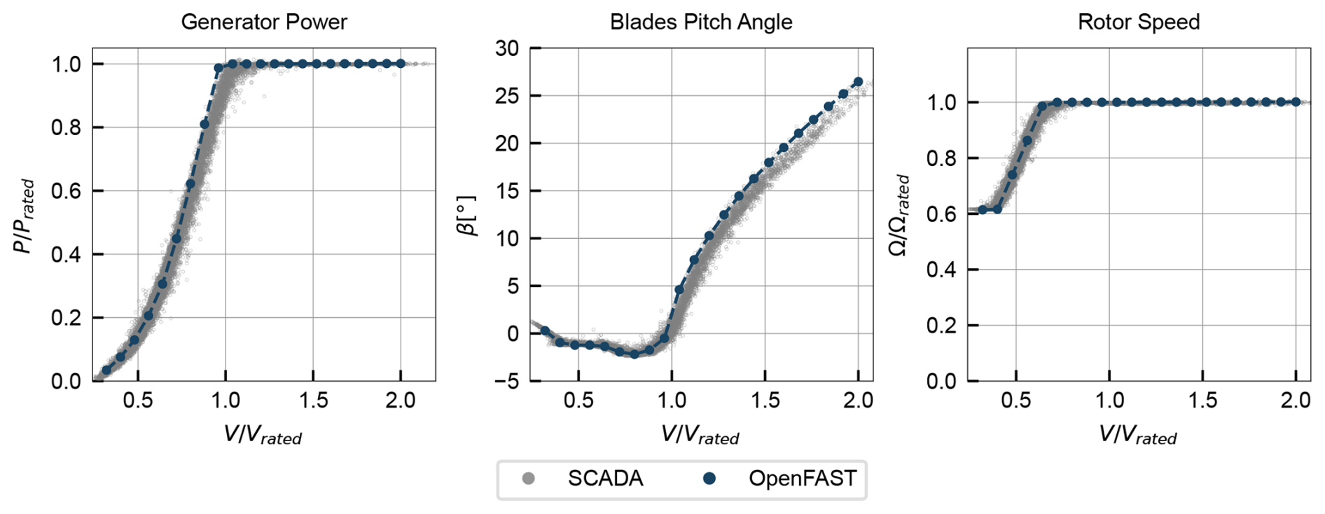
Figure 18 Comparison of simulated operational data under steady wind against 10 min averaged SCADA measurements (baseline model).

The comparison with SCADA data is useful to validate the controller model and perform an initial assessment of the model, but it does not allow a complete evaluation of model accuracy, since it does not provide enough insight into the underlying aerodynamic loads. Furthermore, the power and pitch discrepancies could be attributed to a variety of effects. A further model evaluation and analysis of possible error sources is performed using the SHM measurements, as described in the next section.

6.2 Comparison with tower bending moments

A further assessment of the baseline model is provided by comparing simulated loads against the experimentally obtained loads using the strain gauges in the SHM system described in Sect. 2.3. It is emphasized that, while SCADA data are ubiquitous and relatively easy to obtain, measurements of structural loads are rarer, making this additional dataset valuable to help disentangle different modelling uncertainty sources, which are unclear from SCADA data alone.

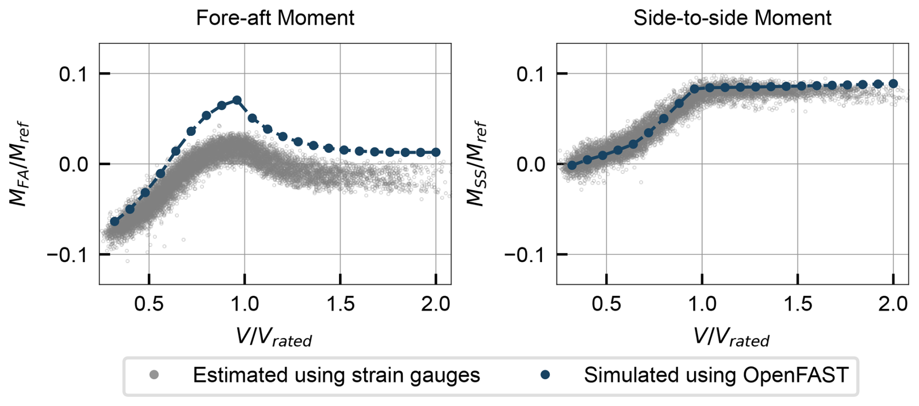
Figure 19 Comparison of simulated loads (baseline model) in cross-section A under steady wind against 10 min averaged loads estimated using the tower strain gauges.

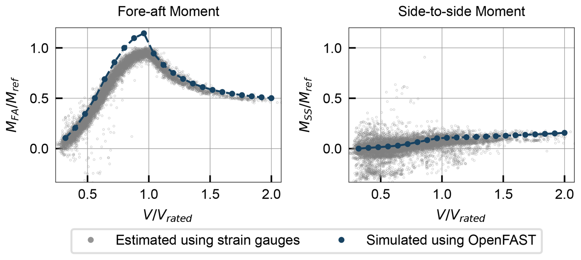
Figure 20 Comparison of simulated loads (baseline model) in cross-section B under steady wind against 10 min averaged loads estimated using the tower strain gauges.

The bending moments at section A are analysed in Fig. 19. The fore–aft bending moment M_FA is overpredicted by the model across the full wind range, although the trend is well captured. The side-to-side bending moment M_SS matches well for almost the entire wind speed range, with a slight overprediction at high wind speeds. Figure 20 shows the bending moments at section B. The fore–aft bending moment M_FA is again overpredicted, especially in below-rated conditions, while there is reasonable agreement in the side-to-side bending moment M_SS. Overall, the fore–aft bending moments have higher errors than the side-to-side moments. The most relevant error is in the fore–aft bending moment at section B below rated wind speed, since it corresponds to an overprediction of the highest magnitude loads experienced by the turbine. Fore–aft bending moments are primarily driven by the rotor thrust, which suggests that the model overpredicts thrust, especially below rated wind speed. This hypothesis is further explored in the next section.

6.3 Comparison with estimated rotor loads

A further comparison is made between experimental and simulated rotor thrust and torque, depicted in Fig. 21. The experimental values were derived from the tower bending moments according to the method in Sect. 3. The simulated values were calculated from the OpenFAST outputs of rotor thrust and torque coefficients. These results summarize the findings from the previous section, providing a more direct insight into the rotor aerodynamic loads: the thrust is slightly overpredicted below rated wind speed, while the torque is reasonably well captured.

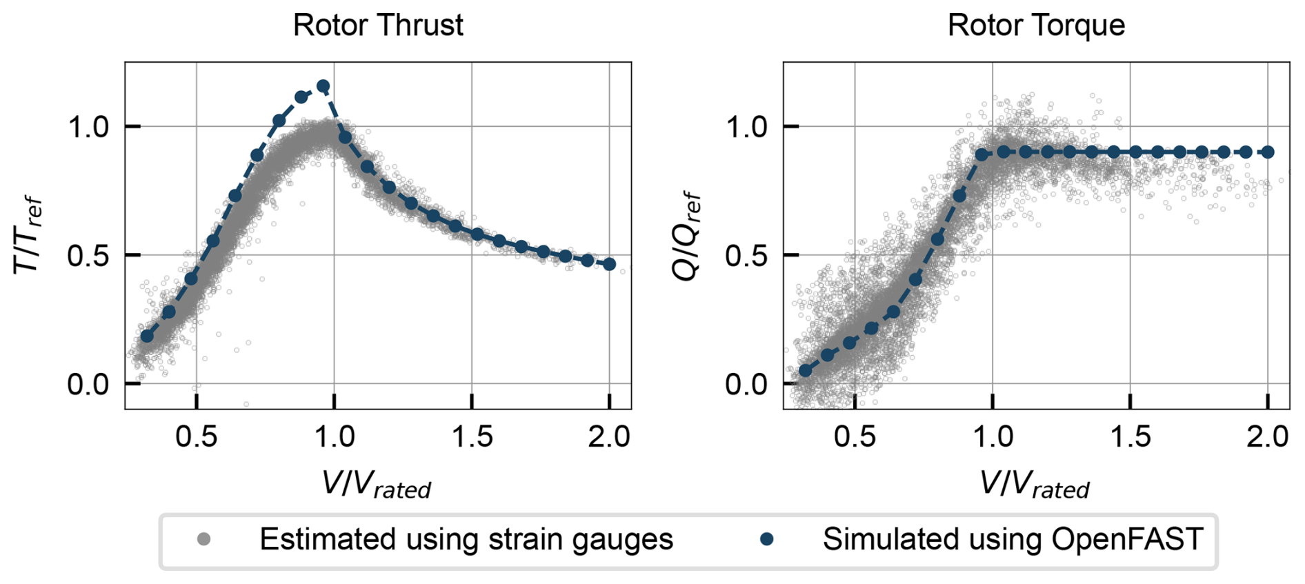
Figure 21 Comparison of simulated rotor loads (baseline model) under steady wind against 10 min averaged loads estimated using the tower strain gauges.

6.4 Effect of turbulence

The above results were obtained assuming steady-wind conditions, often a preferred simulation strategy due to the lower computational cost and post-processing complexity. However, turbulence is always present in real wind conditions, and some of the discrepancies between the simulated curves and the experimental measurements (which correspond to 10 min averages under turbulent wind) may be explained by the effect of turbulence. To assess this, additional simulations were performed including turbulence in the wind field, with turbulence intensities of 5 %, 10 %, and 15 % (corresponding to realistic values of turbulence intensity at the site, as logged by the SCADA system). Turbulent simulation results are compared with the steady-wind results in Figs. 22 and 23 for operational and structural data, respectively.

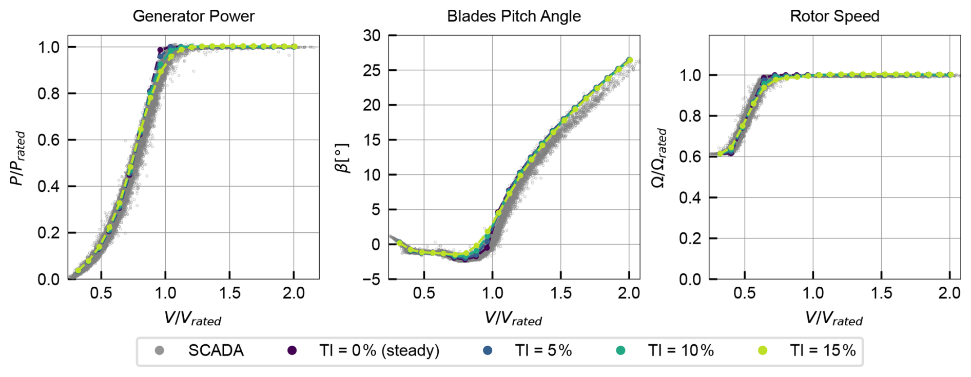
Figure 22 Effect of turbulence intensity on simulated operational data, compared with 10 min averaged SCADA measurements.

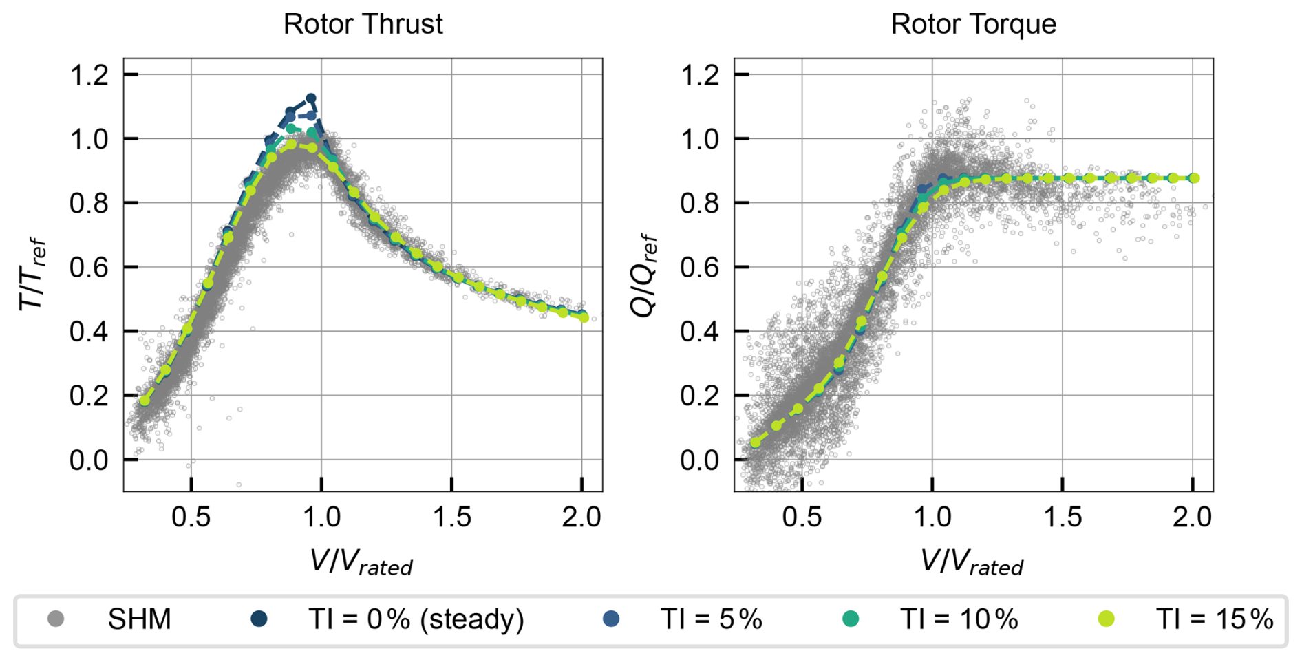
Figure 23 Effect of turbulence intensity on simulated structural data, compared with 10 min averaged SHM measurements.

The comparison with SCADA data shows that the effect of turbulence is relevant only in regions where the controller laws change abruptly, such as around the point where rated power is reached. In these regions, turbulence smooths the transition between different controller regimes, yielding results that are closer to the experimental data. However, away from these regions, the effect of turbulence is negligible, and the steady-wind simulations provide a good approximation of the mean behaviour.

The comparison with SHM data shows a similar trend, where turbulence has a smoothing effect around transition regions. This is especially relevant in the rotor thrust, since this variable peaks around rated wind speed. The apparent overestimation of maximum thrust in the steady-wind simulations is mitigated when turbulence is included, yielding results that are closer to the experimental data. However, below rated wind speed, the thrust is still overpredicted.

6.5 Discussion of baseline results

Overall, the experimental trends observed in both SCADA and SHM data are well captured by the baseline simulations, indicating that the main physical phenomena are represented adequately and supporting the modelling approach. Furthermore, the rotor thrust and torque, estimated with the methods in Sect. 3, served as useful variables to characterize the rotor, summarizing the findings from the tower bending moment comparison and providing a more direct insight into the rotor aerodynamic loads, even without blade instrumentation. This is particularly relevant for the thrust, which is the main driver of the largest tower loads and is not measured in SCADA.

The main observed discrepancies between the model results and the measurements are summarized as follows:

• a slight overprediction of power capture below rated wind speed,

• an overprediction of the rotor thrust below rated wind speed,

• an overprediction of the pitch angle above rated wind speed.

These discrepancies, though small in magnitude, are consistent across both datasets (SCADA and SHM), suggesting inaccuracies in the model rather than errors in the measurements. Furthermore, they appear over the entire wind speed range, rather than being concentrated around specific operating points, indicating that the errors are of a systematic nature and have an underlying physical cause.

The errors suggest an overprediction of the aerodynamic loads: the thrust and power are overpredicted below rated, and the pitch angle is overpredicted above rated, indicating that the simulated turbine maintains rated power with more pitch (i.e. a greater reduction in aerodynamic efficiency) than in reality. This may be explained by modelling errors in the interaction between the wind and the rotor or by errors in modelling the wind field. In other words, there are several model inputs which may explain the observed discrepancies, which motivates a parameter study to assess the sensitivity of the model to selected uncertainties, as described in the next section.

7 Parametric study

7.1 Definition of parameter study

A parametric study was performed to assess the sensitivity of the model to selected uncertainties. A list of parameters which may explain the observed discrepancies was compiled, and each parameter was perturbed individually around the baseline model while keeping all other settings fixed. Parameters characterizing the blade geometry were varied in a range much larger than the expected uncertainty in the laser-scan-based estimates to represent typical uncertainties when laser scans are not available. The parameters considered and their perturbations are listed in Table 1.

Table 1 Parametric study definition.

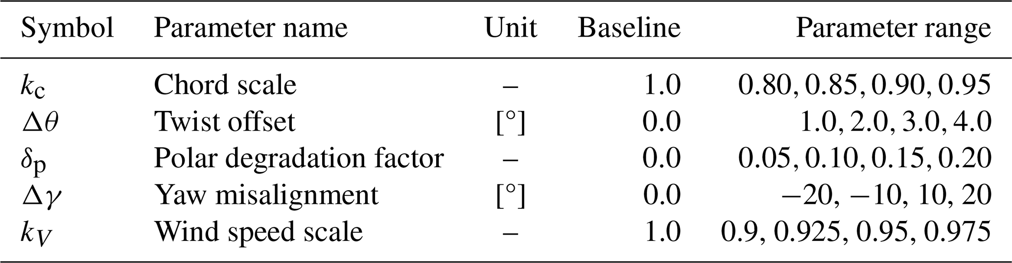
The physical meaning of the selected parameters and their possible relationship with the observed discrepancies are now described.

• Chord scale k_c. As aerodynamic forces are proportional to the blade chord, changes in chord have a direct impact on the rotor's energy capture and loads, suggesting the possibility that the model inputs overestimate the real chord. The chord scale k_c was introduced as a multiplicative factor applied to the entire chord distribution along the blade span, defining new chord distribution $c^{\prime }\left(z_{\mathrm{bld}}\right)=k_{\mathrm{c}}c\left(z_{\mathrm{bld}}\right)$.

• Twist offset Δθ. A second determinant parameter is the blade twist distribution, which directly affects the local angle of attack along the blade span and therefore the aerodynamic performance. Therefore, an offset Δθ was added to the twist distribution (corresponding to a decrease in angle of attack) along the blade span, defining new twist distributions ${\mathit{\theta }}^{\prime }\left(z_{\mathrm{bld}}\right)=\mathit{\theta }\left(z_{\mathrm{bld}}\right)+\mathrm{\Delta }\mathit{\theta }$.

• Polar degradation factor δ_p. The airfoil polars are essential inputs as they directly determine the aerodynamic forces. To account for a possible overestimation of aerodynamic efficiency in the polars, a polar degradation factor δ_p was introduced, which simultaneously decreases the lift coefficient and increases the drag coefficient at all angles of attack. The new polars are defined as $C_{\mathrm{L}}^{\prime }=(\mathrm{1}-{\mathit{\delta }}_{\mathrm{p}})C_{\mathrm{L}}$ and $C_{\mathrm{D}}^{\prime }=(\mathrm{1}+{\mathit{\delta }}_{\mathrm{p}})C_{\mathrm{D}}$.

• Yaw misalignment Δγ. Yaw misalignment reduces the effective wind speed experienced by the rotor, leading to a reduction in energy capture and loads. To assess the possibility of this explaining the observed discrepancies, a yaw misalignment Δγ was introduced in the simulations.

• Wind speed scale k_V. Finally, the possibility of errors in the SCADA wind speed measurement is considered, through a wind speed scale factor k_V, defining new wind speeds $V^{\prime }=k_{V}V$.

It should be noted that other parameters not studied here may also play a role in the observed discrepancies, such as wind shear, drivetrain/generator efficiency, and air density. Nevertheless, the five selected parameters are expected to be the main sources of uncertainty for a typical aeroelastic model.

7.2 Results of parametric study

The results of the parametric study are summarized in Fig. 24, where each row of plots corresponds to one of the parameters listed in Table 1. The three columns correspond to selected outputs as a function of wind speed: generator power, pitch angle, and fore–aft bending moment in cross-section B. Each plot compares simulation results using different parameter values against experimental measurements. The generator power and pitch angle plots are cropped to the wind speed ranges where the respective variables are not set by the controller to focus on the regions where the parameter perturbations have an effect (i.e. below rated for power and above rated for pitch angle). It should be noted that the last row of the plot, which considers variations in the wind speed scale, has the SCADA wind speed V on the x axis, and not the corrected wind speed V^′, to facilitate comparison.

Figure 24 Parameter study results, compared with 10 min averaged SCADA and SHM measurements.

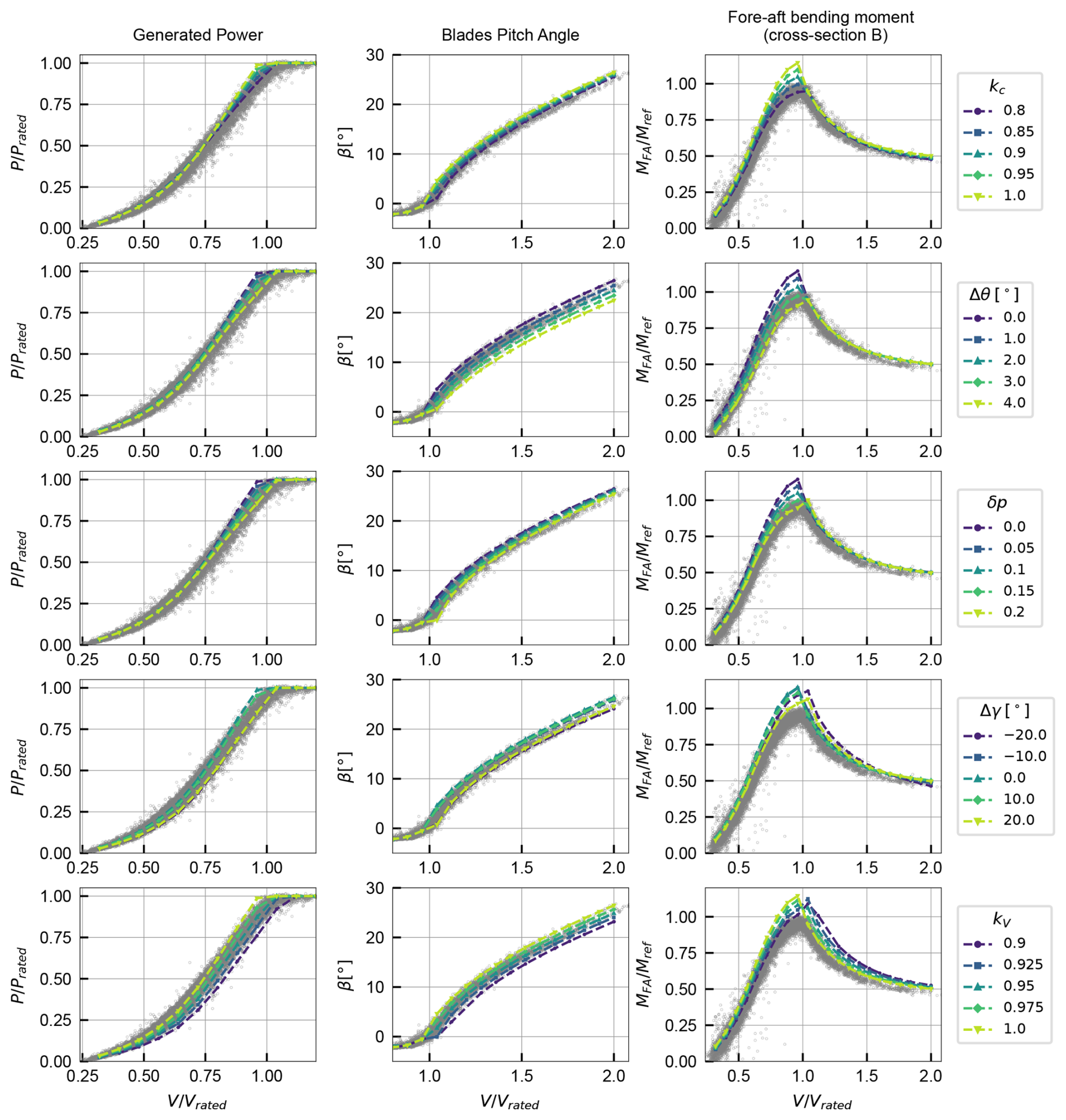
Overall, the figure shows that all parameters have a significant effect on the outputs considered within the ranges studied. In principle, this might allow the tuning of these parameters to match the measurements more closely, but the realism of the required perturbations must be assessed to determine whether these parameters are plausible explanations for the observed discrepancies.

The first two rows in Fig. 24 show the effect of variations in blade geometry through the chord scale k_c and the twist offset Δθ. Both parameters are effective in reducing the observed discrepancies. However, the chord scale necessary to match the measurements (around k_c=0.9) implies a reduction in chord which is much larger than the expected uncertainty in laser-scan-based estimates. Similarly, the twist offset necessary to match the measurements (around Δθ=2°) is also larger than the expected uncertainty in the twist measuring method (described in Fig. 14). In summary, the chord and twist can be tuned to match SCADA and SHM measurements, but the required perturbations are too large to be plausible, given the use of laser scans. This highlights the value of laser scans to reduce uncertainties in blade geometry when validating aeroelastic models, avoiding an incorrect attribution of discrepancies to uncertainties in blade geometry.

The third row in Fig. 24 shows the effect of variations in airfoil polars through the polar degradation factor δ_p. It should be noted that, although the polars are based on the laser-scanned airfoil shapes, they are more uncertain than the chord and twist since they are calculated using XFOIL with additional corrections and extrapolation methods, which may have limitations. Therefore, the polar degradation factor is a more plausible parameter to explain the observed discrepancies. However, the required degradation (around δ_p=0.15) is relatively high, suggesting that other sources of uncertainty may also be relevant.

The fourth and fifth rows of the plot show the effect of yaw misalignment and a scale factor in the measured wind speed, reflecting possible errors in the wind field characterization, a realistic source of uncertainty since the wind field is not measured directly at the rotor, and nacelle-mounted sensors are prone to errors. Both parameters are effective in bringing the simulations closer to the measurements, although an improved match in the power, pitch, and below-rated bending moment comes at the expense of a worse match in the above-rated bending moment.

In summary, the parametric study shows that several parameters can be tuned to reduce the observed discrepancies between the baseline model and the experimental measurements. However, some of these parameters require perturbations larger than the expected uncertainties in the baseline model, suggesting that they are not plausible explanations for the discrepancies. Other parameters, such as the polar degradation factor and wind field characterization, are more plausible sources of uncertainty, although they may not fully explain the discrepancies on their own. This highlights the complex interplay of uncertainties in aeroelastic modelling and the need for comprehensive validation studies using multiple data sources.

8 Conclusions

This study addressed the challenge of accurately predicting the aerodynamic loads in a multi-megawatt wind turbine using aeroelastic models. Typical difficulties, such as the lack of knowledge about blade geometry and the limited measured data available for validation, were addressed using results from experimental campaigns: the terrestrial laser scanning of a wind turbine blade was used to define model geometric inputs, while a tower structural health monitoring system provided additional comparison metrics for model validation.

Terrestrial laser scanning was shown to be a viable approach to reconstructing the outer geometry of wind turbine blades in the absence of detailed manufacturer data. One of the main challenges identified was the presence of blade vibrations during data acquisition, which introduced scatter in the measurements, especially near the blade tip. This was corrected using an alignment procedure, after which the chord, twist, and airfoil shapes were determined by fitting the scan results to airfoils from known families. The zero reference for the twist angle, which significantly impacts simulation results, was established by using laser scan measurements of the nacelle and tower to define the rotor plane.

The structural health monitoring system provided measurements of tower bending moments at two cross-sections. The rotor thrust and torque were estimated from the tower bending moments using a simple static equilibrium model. This provided an additional validation metric beyond SCADA data and a more complete characterization of rotor loads without requiring blade instrumentation.

An OpenFAST model was developed using the scanned chord and twist and XFOIL-generated polars as inputs. Simulation results were obtained under steady and turbulent wind conditions across the operational wind speed range. Overall, there is a good agreement between the model results and the SCADA and SHM data. Some discrepancies were identified, namely a slight overprediction of rotor aerodynamic loads, which manifests itself in the SHM data as an overestimation of thrust below rated power and in the SCADA data as an overestimation of pitch for rated-power conditions. A parametric study was performed to assess the sensitivity of the model to selected inputs to investigate possible error sources, showing that inputs of a different nature can impact the model results similarly. A mixture of different uncertainty sources is likely to explain the observed discrepancies, with the polar calculation and the wind field measurement being plausible contributors. Due to the use of laser scans, the blade geometry is unlikely to be a significant source of error.

A natural next step targeting improvement in load predictions would be to perform a constrained optimization of uncertain model inputs, using realistic parameter bounds informed by the available measurements and using SCADA and SHM data as simultaneous objectives. For a more holistic modelling improvement aiming at, for example, lifetime estimation, the next main step is not to further tune the aerodynamic model, but rather to calibrate the structural part of the model (e.g. blade mass and stiffness distributions), gaining insight into the structure's response to the already adequately modelled aerodynamic loads.

Overall, the results highlight the value of experimental measurements for developing and validating aeroelastic models. The laser-scanned geometry provided a realistic representation of the blade geometry, enabling a more reliable attribution of discrepancies to other sources of uncertainty. The SHM measurements provided additional validation metrics beyond SCADA data, allowing for a more comprehensive assessment of the model's ability to predict structural loads.