Investigating the wind–wave interaction on mean wind and turbulence structure using COAWST with WRF-LES during a storm event

We investigate wind–wave interactions within the marine atmospheric boundary layer during a storm event over the North Sea using a multiscale coupled modeling framework. Large-eddy simulation (LES) domains within the Weather Research and Forecasting model have been coupled with the Simulating WAves Nearshore (SWAN) model through the Coupled Ocean–Atmosphere–Wave–Sediment Transport (COAWST) system. The simulation consists of six nested domains, three outer mesoscale domains with horizontal grid spacings of 9.9, 3.3, and 1.1 km and three inner large-eddy simulation domains with coarse (100 m) and fine horizontal grid spacings. Wind and wave outputs from both the finest mesoscale domain and the coarsest LES domain are evaluated against metocean and lidar measurements collected during the storm. The results show that the coarsest LES domain represents wind speeds up to 150 m height more accurately than the mesoscale output, which is however associated with excessive simulated vertical wind shear. Above this height, the mesoscale and LES winds become much closer, both overestimating the measured winds. The measured wind direction is well captured across all domains. The significant wave height, peak wave period, and mean wave direction simulated by SWAN show better agreement with observations when forced by the LES output than the mesoscale output. Additionally, the coupled simulations exhibit stronger turbulence fluxes than the uncoupled simulations, which is clearly shown in the vertical profiles of velocity variances and covariances. Although it is a case study, these findings demonstrate the impact of high-resolution coupled modeling for capturing offshore boundary layer dynamics and on wind and wave predictions under severe weather conditions.

1 Introduction

Accurate understanding of the structure of the marine atmospheric boundary layer (MABL), including mean wind profiles and turbulence characteristics, has become increasingly important in recent decades due to the global expansion of offshore wind energy. The physical processes in the MABL can be more complex than those over land due to additional interactions at the air–sea interface, which span multiple temporal and spatial scales. These interactions, particularly involving ocean waves, can modify the atmospheric flow up to hub height and above (Kalvig et al., 2014; Yang et al., 2014; Fischereit et al., 2022), affecting wind resource assessments, turbine loading, and energy yield predictions. Such complexities require advanced, high-resolution modeling strategies, which were listed as key scientific challenges for offshore modeling in Shaw et al. (2022).

Atmospheric motions within the MABL are impacted by mesoscale weather systems down to turbulent eddies. Numerical models are typically designed to operate at a range of scales, and as a result, studies often rely on a variety of parameterizations and configurations to bridge the gap between mesoscale and microscale dynamics (Chow et al., 2019). Our understanding of coupled wind–wave dynamics has been limited to a high degree by the difficulty of calculating mesoscale weather variability and microscale turbulence simultaneously over realistic ocean surfaces. To address this, as one of the few studies, Ning et al. (2023) evaluated parameterizations of sea surface roughness in a multiscale simulation framework. They employed the Weather Research and Forecasting (WRF) model coupled with the Simulating of WAve Nearshore (SWAN) model for mesoscale processes and fed the output of the wave-influenced roughness parameterization into the parallelized large-eddy simulation model (PALM). Their results showed that, although the framework reproduced mean wind and turbulence characteristics under realistic offshore conditions, it exhibited minimal sensitivity to the different roughness parameterizations. Additionally, their use of a one-way, meso-to-micro coupling meant that interactions between meso- and microscales were not accounted for. They suggested that future work should explore two-way coupling strategies and more advanced wind–wave parameterizations.

The technical challenges associated with such modeling underscore the need for a multiscale modeling framework that integrates mesoscale and microscale processes. Such a modeling framework would allow for nesting large-eddy simulation (LES) domains within mesoscale simulations, enabling the representation of both synoptic-scale variability and turbulence. In these frameworks, mesoscale atmospheric conditions provide realistic time-varying boundary forcing for the embedded LES, allowing us to partly resolve turbulence with the possibility of wave-induced feedback that would otherwise be missed in coarser simulations. Multiscale simulations driven by time-varying atmospheric conditions have been shown to be able to represent meteorological processes on land with large-scale variations in wind and temperature, as well as the associated turbulent flow structures across scales (Muñoz-Esparza et al., 2017). Here we want to extend the meso-to-micro coupling to offshore conditions, where both the mesoscale and the LES domains are explicitly coupled with a wave model to represent wind–wave interactions in the MABL, which has not been fully addressed in earlier multiscale studies. We use the Coupled Ocean–Atmosphere–Wave–Sediment Transport (COAWST) modeling system (Warner et al., 2010). COAWST is a well-established tool for simulating air–sea interactions. The COAWST framework integrates several modeling components comprising the model coupling toolkit to exchange data fields between an ocean model (ROMS), an atmospheric model (WRF), a wave model (SWAN), and a sediment transport model. Numerous studies have utilized COAWST to investigate a variety of air–sea interaction processes (Cambazoglu et al., 2024; Jiang et al., 2025). To our knowledge, to date, all coupling between the components of the WRF and SWAN models within the COAWST framework has been performed at mesoscale resolutions. For example, in the field of offshore wind energy, studies have examined interactions between wind, waves, and wakes (Larsén et al., 2024; Fischereit et al., 2022), while others have focused on hurricanes and extreme tropical cyclones (Chen et al., 2024; Alimohammadi et al., 2020; Olabarrieta et al., 2012). Larsén et al. (2019) used COAWST to compare roughness length parameterizations with direct stress coupling for wave–atmosphere interactions. They found that stress-based coupling better captured the wind field measured by synthetic aperture radar over a coastal, shallow water area.

Here, we focus on exploring the multiscale model system's capability through an extreme wind and wave event, following our previous study (Hamzeloo et al., 2025), in which we investigated the effects of waves on mean wind speed, direction, turbulence fluxes, and spectral characteristics using a one-way offline coupling between WRF-LES and the MIKE3 Wave FM model (M3W) (DHI, 2024). The study in Hamzeloo et al. (2025) was conducted under idealized conditions. Here, we build on that work by performing a fully coupled weather-driven multiscale simulation using WRF and SWAN through COAWST, allowing for a more realistic assessment of wave effects on MABL dynamics.

This paper is structured as follows: Sect. 2 describes the methodology, including a description of the measurement data, the model setup for both wind and wave components, and the coupling strategy. Section 3 presents the simulation results. Sections 4 and 5 provide discussion and conclusions, respectively.

2 Methodology

2.1 Measurements and the selected case

We use wind and wave measurements from the Reducing the Uncertainty of Nearshore Experiment (RUNE) project to evaluate wind and wave simulations. RUNE was a collaborative research project that conducted a coastal offshore measurement campaign from 2 November 2015 to 1 March 2016, near the west coast of Jutland, Denmark. The experiment and data collected during RUNE are described in detail by Floors et al. (2016) and Bolaños and Rørbæk (2016).

During the campaign, wind and wave measurements were taken approximately 7 km offshore. Wave measurements were obtained using a directional Triaxy wave buoy equipped with a downward-looking acoustic Doppler current profiler. This buoy was deployed at the beginning of the campaign at a water depth of 16.5 m. The hourly integrated wave parameters – including significant wave height (H_s), maximum wave height (H_max), peak wave period (T_p), average zero-crossing period (T₀₂), and mean wave direction (MWD) – are processed from the 7 Hz sampled data. A lidar buoy, positioned less than 200 m from the wave buoy, was equipped with a WindCube^® v2 Doppler wind lidar to record wind data. Mean wind speed and direction are available every 10 min at 12 different heights above the mean sea level: 40, 47, 59, 79, 97, 117, 134, 147, 172, 197, 209, and 247 m. Figure 1 shows the geographical location of the RUNE measurements as a red dot.

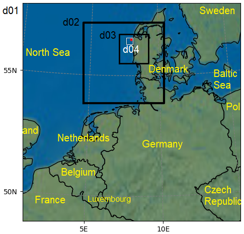
Figure 1 Nested domains' configuration of our simulations. The red dot in the upper right of domain D04 is the location of the RUNE measurements. Domains D05 and D06 located within D04 are not shown.

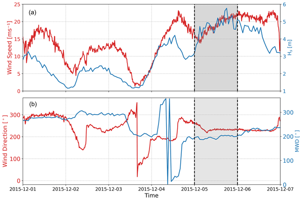
Figure 2 presents the time series of H_s and the wind speed at a height of 40 m, MWD, and the wind direction at a height of 40 m for a period of a week around our focus day, 5 December 2015. The wind measurements shown in the plots correspond to the lowest recorded height. We observe an overall wind–wave alignment from the southwest (less than 60° difference), which lasts for almost a full day on the focus day, marked in gray in Fig. 2. Additionally, the most intense wave event during the measurement period occurred on the same day at 18:00 UTC, with H_s=5.77 m and T₀₂=8.7 s. During this storm, the average wind speed ranged from 21.3 m s⁻¹ at 40 m to 26.8 m s⁻¹ at 247 m. We use this day to investigate the wind–wave interaction in the COAWST modeling system in LES mode.

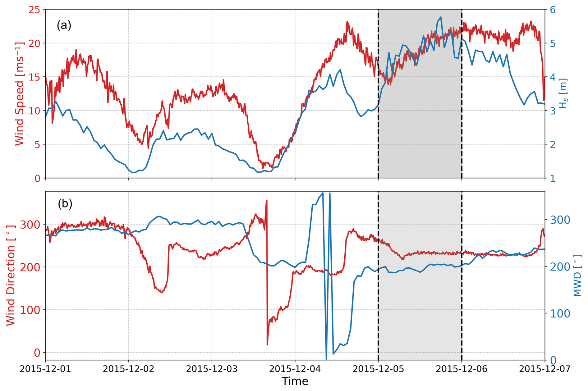
Figure 2 Time series of wind speed (a) and direction (b) on the left axis and significant wave height H_s (a) and mean wave direction (MWD) (b) on the right axis, from measurements of the wave buoy and the lidar at a 40 m height, respectively. The gray range shows the period we selected for this study.

2.2 Modeling system

We utilize the WRF model, version 4.5 (Skamarock et al., 2019), and SWAN model, version 41.45 (Booij et al., 1997), through the COAWST modeling system version 3.8 (Warner et al., 2010) to simulate wind–wave interactions in the North Sea for the selected storm. Other components of the COAWST system are not activated in this study. The WRF and SWAN models are two-way, online, coupled through the wave boundary layer model (WBLM) implemented in SWAN (Du, 2017; Du et al., 2019). The WBLM accounts for the vertical variation in stresses and energy in the wave boundary layer (WBL), which is the interface between the waves and the atmospheric boundary layer. In this layer, the wind speed profile deviates from the classical logarithmic shape due to wave-induced motions and momentum exchange. In this coupled system, the WRF horizontal velocity components at a height of 10 m (longitudinal U and meridional V) are sent to SWAN. The WBLM uses the former velocities along with local wave-induced and turbulent stress, as well as wave phase velocity, to calculate the vertical wind profile within the WBL by solving the kinetic energy conservation equation; computes the equivalent roughness length (z₀) that conforms to the logarithmic wind profile; and finally transfers z₀ back to the surface layer module of the WRF model (Du et al., 2022; Fischereit et al., 2022). For the uncoupled WRF simulations, the surface layer parameterization relies on the revised MM5 Monin–Obukhov scheme (Jiménez et al., 2012), which uses the default Charnock-based formulation (Charnock, 1955) in its revised form following Fairall et al. (2003) to diagnose the sea surface roughness length, computed as

$$\begin{array}{}\text{(1)}& z_{\mathrm{0}}={\displaystyle \frac{\mathit{\alpha }{u}_{*}^{\mathrm{2}}}{g}}+{\displaystyle \frac{\mathrm{0.11}\mathit{\nu }}{u_{*}}},\end{array}$$

where the Charnock parameter α is a function of the 10 m wind speed U₁₀,

$$\begin{array}{}\text{(2)}& \mathit{\alpha }=\left\{\begin{array}{ll}\mathrm{0.011},& U_{\mathrm{10}}<\mathrm{10}\mathrm{m}{\mathrm{s}}^{-\mathrm{1}}\\ \mathrm{0.011}+\frac{\mathrm{0.018}-\mathrm{0.011}}{\mathrm{18}\mathrm{m}{\mathrm{s}}^{-\mathrm{1}}-\mathrm{10}\mathrm{m}{\mathrm{s}}^{-\mathrm{1}}}\\ \times (U_{\mathrm{10}}-\mathrm{10}\mathrm{m}{\mathrm{s}}^{-\mathrm{1}}),& \mathrm{10}\mathrm{m}{\mathrm{s}}^{-\mathrm{1}}\le U_{\mathrm{10}}\le \mathrm{18}\mathrm{m}{\mathrm{s}}^{-\mathrm{1}}\\ \mathrm{0.018},& U_{\mathrm{10}}>\mathrm{18}\mathrm{m}{\mathrm{s}}^{-\mathrm{1}}\end{array}\right.,\end{array}$$

and u_* is the friction velocity, g is the gravitational acceleration, and ν is the kinematic viscosity of air. The second term accounts for viscous effects and becomes important under weak wind conditions.

Therefore, the results from coupled WRF–SWAN simulations consider realistic wave growth and improved energy exchange at the air–sea interface compared to the uncoupled simulations.

Unlike most previous COAWST applications, which remain limited to mesoscale resolutions, our configuration extends the coupling to include LES domains. To make this framework operational, we applied two key adjustments. First, in domains with finer horizontal grid spacing than 100 m, we replaced the planetary boundary layer (PBL) scheme with LES. Second, we implemented the cell perturbation method (CPM) (Muñoz-Esparza et al., 2015; Muñoz-Esparza and Kosović, 2018) in the WRF model within the COAWST framework to enable turbulence simulations.

2.3 Simulations

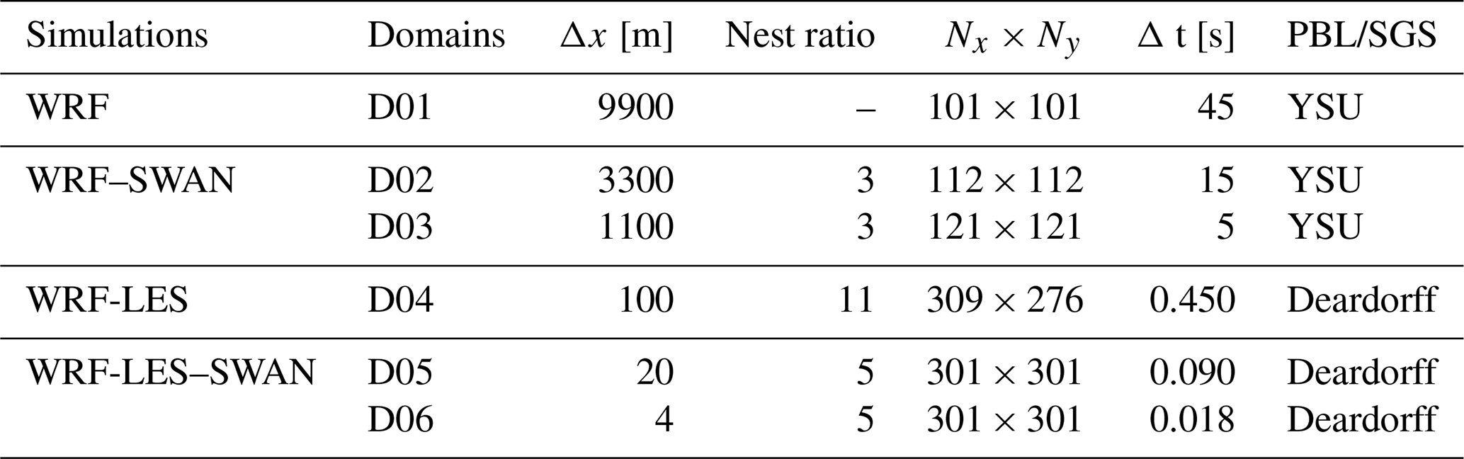
Our multiscale WRF simulations include six nested domains. The outer three domains run in mesoscale mode with horizontal grid spacings of 9.9, 3.3, and 1.1 km, denoted as D01, D02, and D03, respectively, while the inner three domains run in LES mode (denoted as D04, D05, and D06). The coarsest LES domain D04 has a grid spacing of 100 m. The grid spacing ratio between mesoscale domains is 1:3, while the ratio from the finest mesoscale D03 to the coarsest LES domain D04 is 1:11. In addition, we nest two more LES domains D05 and D06 with a 1:5 grid spacing ratio of 20 and 4 m, which are run for a shorter period (10 h). The time step ratio matches the grid spacing ratio, with a time step of 45 s for the outermost mesoscale domain. All six domains consist of 61 vertical levels, with the first level located at 10 m above the surface. The model's top is at 5000 Pa. The SWAN model adopts the same domain configuration as presented in Fig. 1. More details on the model domain specifications can be found in Table 1. Both coupled and uncoupled simulations employ the same domain configuration, nesting ratios, input data, and physical parameterizations. The simulations differ only in that the uncoupled simulation includes only the atmospheric model (WRF), whereas the coupled simulations additionally incorporate the wave model (SWAN).

A grid spacing of 100 m is intentionally used for the LES domain D04, as it reflects what is commonly used in industry and operational multiscale modeling (Vortex FdC, 2018; Kshetri and Momen, 2025), where computational constraints limit the LES domain sizes. Although the LES domains use a 1.5-order turbulence kinetic energy (TKE)-based subgrid-scale (SGS) model (Deardorff, 1980), the coarse horizontal grid spacing only allows a limited portion of the turbulence field to be explicitly resolved for this particular storm event, and therefore, a substantial fraction of the turbulent stresses originate from the SGS model. The finer-resolution LES domains (D05 and D06) are included to partly demonstrate how higher resolution increases the fraction of resolved turbulence.

Table 1 Domain configurations of the simulations. Δx corresponds to horizontal grid spacing, N_x and N_y to number of grid points in the x (west–east) and y (north–south) direction, and Δt to numerical integration time step.

The outermost domain is initialized and forced using ERA5 reanalysis data, updated every 6 h (Copernicus Climate Change Service, Climate Data Store, 2017). In addition, the Operational Sea Surface Temperature and Sea Ice Analysis (OSTIA) dataset (Donlon et al., 2012) is used to update the sea surface temperature and sea ice fields during simulations every 6 h. For static inputs, we utilize the default datasets provided by the WRF model, along with the CORINE land cover dataset (Feranec, 2016) and the ESA Climate Change Initiative (CCI) land cover datasets at resolutions of 100 and 300 m, respectively (Bontemps et al., 2013).

For the physics parameterizations of the WRF model, we employ the WRF Single-Moment 6-Class (WSM 6-class) graupel scheme for microphysics (Hong et al., 2004), which includes predictive variables for water vapor, cloud water/ice, rain, snow, and graupel. For radiation processes, we utilize the Rapid Radiative Transfer Model (RRTM) (Mlawer et al., 1997) for longwave radiation and the Dudhia scheme (Dudhia, 1989) for shortwave radiation, both executed every 9 min. The Kain–Fritsch scheme (Kain and Fritsch, 1993) is employed for cumulus parameterization, activated every 5 min exclusively for the outermost domain. The Unified Noah land surface model (Tewari et al., 2004) is applied for land surface, while the revised MM5 Monin–Obukhov scheme is used for the surface layer (Jiménez et al., 2012). The Yonsei University (YSU) scheme (Hong et al., 2006) is used for PBL parameterization, which was selected based on a sensitivity analysis among three other schemes: the Mellor–Yamada–Nakanishi–Niino (MYNN) (Nakanishi and Niino, 2006), Mellor–Yamada–Janjic (MYJ) (Janjic, 1996), and quasi-normal scale elimination (QNSE) (Sukoriansky et al., 2005) schemes. PBL schemes are deactivated for the innermost domains as they run in LES mode. The SGS model prognoses the TKE, which is used to compute the local eddy diffusivity.

The SGS part of the stress includes the deviatoric component ${\mathit{\tau }}_{ij}^{\text{dev}}$ and the part from the SGS turbulent kinetic energy e_sgs. Using the 10 s model outputs (D04 outputs e_sgs and the deviatoric stresses), the SGS stress is calculated as

$$\begin{array}{}\text{(3)}& {\mathit{\tau }}_{ij}^{\text{sgs}}={\displaystyle \frac{\mathrm{2}}{\mathrm{3}}}{\mathit{\delta }}_{ij}{e}_{\text{sgs}}+{\mathit{\tau }}_{ij}^{\text{dev}}.\end{array}$$

The resolved stress components (${\mathit{\tau }}_{ij}^{\mathrm{res}}$) for each velocity pair are computed as

$$\begin{array}{}\text{(4)}& {\mathit{\tau }}_{ij}^{\text{res}}=-\mathit{\rho }\langle u_i^{\prime }{u}_j^{\prime }\rangle ,\end{array}$$

where ρ is the air density; u_i and u_j are the along-wind and cross-wind components; the primes (^′) denote fluctuations from the mean value, which are computed as a 10 min time average at the grid point closest to the measurement site; and the angle brackets 〈⋅〉 indicate a temporal average. The total stress components are obtained from

$$\begin{array}{}\text{(5)}& {\mathit{\tau }}_{ij}^{\text{tot}}={\mathit{\tau }}_{ij}^{\text{res}}+\langle {\mathit{\tau }}_{ij}^{\text{sgs}}\rangle .\end{array}$$

In multiscale simulations using the WRF model, turbulence in the LES domain may not develop fast enough because of the smooth flow from the parent mesoscale domain and the time needed for high-resolution LES domains to develop turbulence. In contrast to the PBL scheme used within mesoscale domains, within the LES domains turbulence is partially resolved, and the SGS model represents the unresolved subgrid-scale turbulence, which further contributes to the Reynolds stresses and TKE (Muñoz-Esparza et al., 2014). This challenge is more significantly intensified in offshore areas, where the absence of topographical features limits the production of turbulence. To address this issue and promote a seamless transition from mesoscale boundary conditions to fully developed LES turbulence, the CPM is applied at the inflow boundaries of the LES domain. In this study, for the first time, we integrate the CPM into the WRF model within the COAWST framework, enabling the application of this technique in coupled ocean–atmosphere–wave simulations. The CPM method (Muñoz-Esparza et al., 2015) introduces controlled perturbations on the potential temperature field. We apply the perturbations on three contiguous cells of the lateral boundaries to develop realistic turbulent fields (Peña and Mirocha, 2024). Additionally, we conduct a simulation without activating CPM in the LES domain D04 to assess its impact on the simulations, which is presented in Sect. 3.5.

For the wave modeling, we initialize the SWAN model using the output spectrum at each grid cell from a previous simulation conducted 24 h earlier to allow for spin-up and provide consistent boundary and initial conditions. The open boundaries of the outermost domain are set to zero. This does not impact the innermost domains due to the large domain size. We utilized 36 directional bins with a frequency exponent of 1.1. The frequency range extends from 0.03 to 10.05 Hz, resulting in a total of 61 frequency bins. The SWAN model operates with a time step of 6 min for the four outermost domains, and the time step is reduced to 4 min for D05 and D06. The EMODnet digital terrain model (DTM) with a grid resolution of $\mathrm{1}/\mathrm{8}$ arcmin (approximately 230 m) is used for the bathymetry. In addition to the configurations mentioned above, the SWAN model incorporates several physical processes to accurately simulate wave dynamics relevant for our model domain, which is in the coastal zone with relatively shallow water. The depth-induced wave breaking is calculated using the parameters α=1.0 and γ=0.73, which control the intensity and the break threshold, respectively. Bottom friction is taken into account using the JONSWAP formulation with a friction coefficient of 0.038, representing energy dissipation due to seabed interactions. White-capping dissipation, which addresses the energy loss from wave breaking in deep water, is activated using the WAM Cycle 3 formulation with drag law fitting. In addition, SWAN considers processes related to sea spray, specifically by modeling white capping and wave-induced breaking. In the present coupled configuration, the effects of sea spray on atmospheric enthalpy fluxes and momentum exchange are indirectly represented through modifications of surface roughness and stress in the surface layer scheme. As the ocean component in COAWST is not activated, ocean mixing and feedback through sea surface temperature (SST) modification are not considered.

Coupled and uncoupled simulations for D01 to D04 are run over a 30 h period from 18:00 UTC on 4 December to 00:00 UTC on 6 December. Coupled and uncoupled simulations for D05 and D06 are run for a shorter period of 10 h with the same starting time. Results and analysis focus on all of 5 December for D01 to D04 and on the first 4 h of this day for D05 and D06, which we use for turbulence analysis. The SWAN model outputs are saved every 10 min for both D03 and D04. For the WRF model, outputs were saved every 10 min for D03 and every 10 s for D04, D05, and D06. All domains share the same spin-up period, despite the shorter total simulation time of D05 and D06.

3 Results

In this section, we first present the surface roughness length (z₀) fields from the finest mesoscale domain (D03) and the coarsest LES domain (D04) for both the coupled and uncoupled simulations, as z₀ is the key parameter connecting the wave and atmospheric field. This allows us to quantify the effect of the WBLM on the surface layer properties before analyzing its effect on the atmosphere (Sect. 3.1). We then evaluate the outputs from the WRF and SWAN models by comparing simulated wind and wave data from D03 and D04 with RUNE observations at the grid point closest to the measurement site (Sect. 3.2 and 3.3). After the validation, we analyze the turbulence fluxes from D04, D05, and D06 (Sect. 3.4). The results from D05 and D06 are not used for validation, as these domains run only for a shorter period, and their purpose is to illustrate the effect of horizontal grid spacing on the resolved and SGS contributions to turbulence.

3.1 Surface roughness

Figure 3 shows distributions of the computed roughness length on 5 December for D03 and D04 from the coupled and uncoupled simulations. The distributions are computed from an area of 6 × 6 grid points in D03 and the corresponding 66 × 66 grid points in D04 around the RUNE location. The figure illustrates the effect of coupling and horizontal resolution on the variability and distribution of roughness length. Overall, mesoscale domains correspond to larger z₀ than the LES domains. The atmosphere-only, non-coupled simulations also give larger z₀. The shapes of WRF‐LES and WRF-LES–SWAN distributions differ: WRF-LES appears narrow and Gaussian, while WRF-LES–SWAN is broader and appears Weibull-like. Similarly, for the mesoscale data, the coupled WRF–SWAN also shows more variability compared to WRF. The differences are mainly due to the method used to calculate the sea surface roughness length in the coupled and uncoupled models. In the coupled system, roughness is dynamically derived from the wave state via the WBLM (Du et al., 2019), whereas in the uncoupled WRF simulations, it is described by Eq. (1).

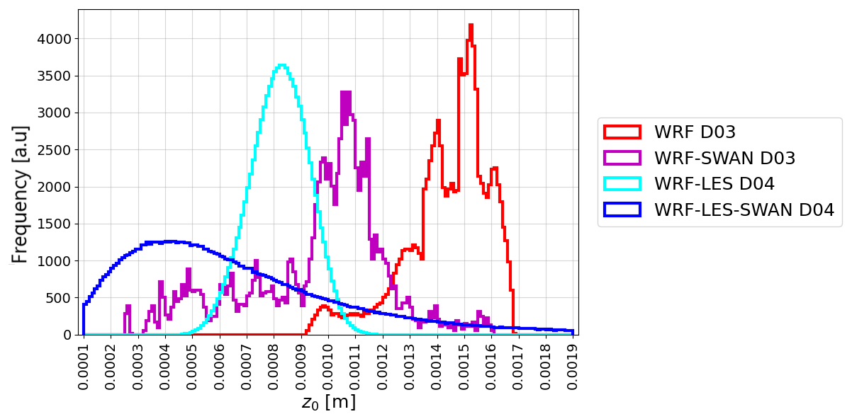
Figure 3 Distributions of simulated roughness length for D03 and D04 from coupled and uncoupled simulations for 5 December, taken from several grid points around the RUNE locations.

3.2 Evaluation of simulated wave parameters

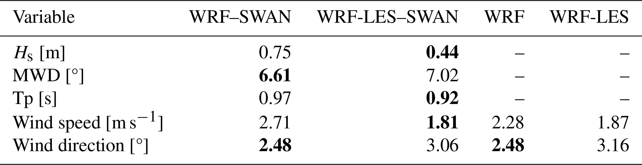
Figure 4 presents a comparison of H_s, MWD, and T_p derived from SWAN when coupled with both the mesoscale (D03) and LES (D04) domains against RUNE buoy measurements. The 10 min simulation outputs were averaged over hourly intervals to match the temporal resolution of the hourly integrated measured wave parameters. The corresponding values of the root mean square error (RMSE) for each domain, calculated relative to the observations, are summarized in Table 2. The results indicate that, while model outputs in both domains follow the observed data, the LES-driven output provides improved wave characteristics, particularly for H_s, with an RMSE nearly half that of the mesoscale-driven domain output. The simulated T_p and MWD exhibit only minor differences between the two domains.

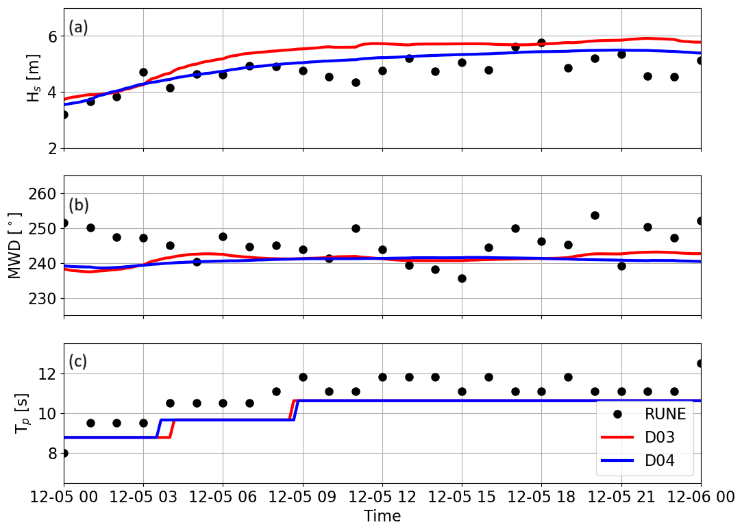
Figure 4 Hourly averaged time series of significant wave height (H_s) (a), mean wave direction (MWD) (b), and peak wave period (T_p) (c) from the coupled simulations of the mesoscale-driven (D03) and LES-driven (D04) domains, compared to wave buoy measurements on 5 December.

Table 2 The root mean square error (RMSE) computed between observations and simulations. The simulated significant wave height (H_s), mean wave direction (MWD), peak period (Tp), wind speed, and wind direction are from the D03 and D04 model outputs. WRF and WRF–SWAN are taken from D03 for the uncoupled and coupled simulations, while WRF-LES and WRF-LES–SWAN are taken from D04. The wind speed and direction statistics are calculated for each of the heights from 40 up to 147 m and then averaged. Bold numbers indicate the lowest RMSE.

3.3 Evaluation of simulated mean flow

The time series of mean wind speed and direction output from both the coupled WRF–SWAN and WRF-only simulations of the mesoscale D03 domain and the LES D04 domain are compared against the lidar measurements at four different heights, 40, 79, 97, and 147 m, in Fig. 5. To ensure temporal consistency with the mesoscale results and measurements, the LES outputs were averaged over 10 min intervals from the 10 s output. At 40 m (Fig. 5a4), the lowest measurement height, simulations from the LES domain (both WRF-LES–SWAN and WRF-LES) show better agreement with observations than those from the mesoscale domain, in terms of magnitude and variability. At 79 m (Fig. 5a3), the WRF-LES–SWAN run exhibits the best agreement with measurements. Above 97 m, WRF-LES–SWAN tends to overestimate the wind speed compared to observations, and at 147 m, the WRF-LES run also overestimates the observed wind speed, which can primarily be attributed to the effect of boundary conditions, as ERA5 overestimates the measurements by up to 3 m s⁻¹ at some time steps. The higher simulated wind speeds in the coupled versus uncoupled simulations and the LES versus mesoscale simulations are consistent with the decreased simulated roughness length as shown in Fig. 3.

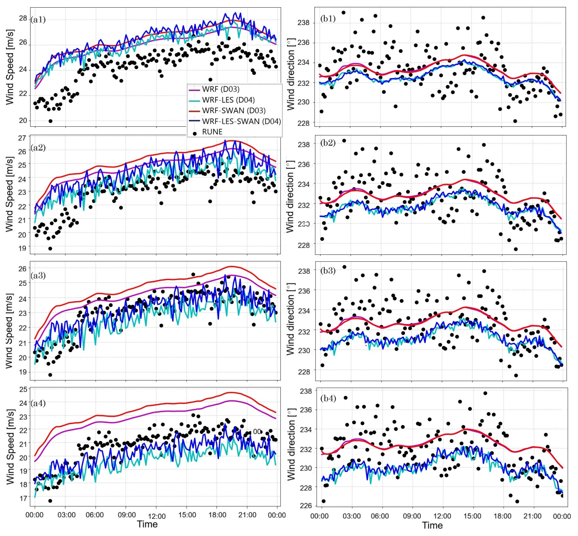
Figure 5 Time series of 10 min means of simulated (left column) wind speed and (right column) wind direction from the mesoscale (D03) and LES (D04) domains for both coupled (WRF–SWAN) and uncoupled (WRF) simulations, compared to lidar buoy data, over the period 00:00 to 23:59 UTC. The left frames (a1–a4) correspond to wind speed at heights of 147, 97, 79, and 40 m, respectively. The right frames (b1–b4) show wind direction at the same heights.

Figure 6 presents the vertical profiles of wind speed and direction during the 2 h period surrounding the time of maximum wave height (hours 17:00 to 19:00 UTC in Fig. 2). Both WRF-LES and WRF-LES–SWAN simulations provide wind speeds lower than observations near the surface; however, they result in an overall good agreement with measured mean wind speed between 40 and 150 m, as also evident in the RMSE values (Table 2) and the time series (Fig. 5). However, this is likely due to excessive vertical wind shear, which is attributed to the type of SGS model used for the LES domains (Peña and Mirocha, 2024; Sullivan et al., 1994; Gadde et al., 2021). In contrast, WRF and WRF–SWAN show wind profiles with vertical wind shears that are more consistent with those from the measurements, although both have a systematic bias at all measured levels. In addition, slightly higher wind speeds are observed in the coupled simulations compared to the uncoupled ones. The WBLM, which accounts for wave impacts and calculates an effective roughness length, yields lower roughness length values than those from the Charnock-based parameterization used by default in the WRF model, particularly under storm conditions. This is reflected in the analysis in Fig. 3. Similar results were previously reported in Larsén et al. (2019) under stormy conditions. Lower roughness lengths lead to higher surface wind speeds under the same forcing conditions. In terms of wind direction, both WRF-LES and WRF-LES–SWAN runs show a slight eastward deviation, with a maximum of approximately 4° up to 100 m.

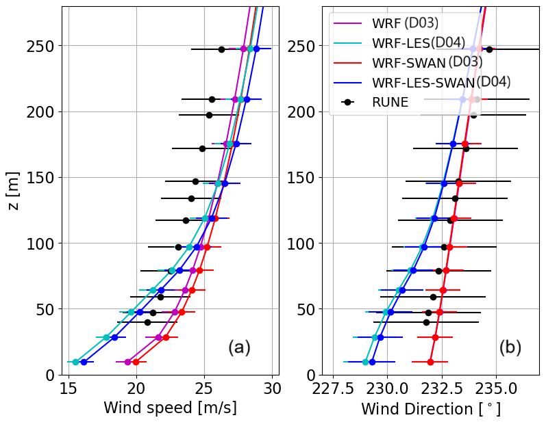
Figure 6 Vertical profiles of (a) wind speed and (b) wind direction over the period 17:00 to 19:00 UTC from the D03 and D04 domains, for both coupled and uncoupled simulations, compared with lidar buoy measurements from 17:00 to 19:00 UTC.

3.4 Turbulent fluxes

Although no high-frequency measurements are available for in-depth validation of the LESs of turbulence, we investigate the behavior of turbulent fluxes of the coupled and uncoupled simulations using results from the LES domains. For this, we compute both the resolved and the SGS stress components. To capture the extreme event at the RUNE measurement location, we use 10 s model outputs over a 2 h period from 02:00 to 04:00 UTC.

Figure 7 shows the vertical profiles of the velocity variances $\langle u^{\prime }{u}^{\prime }\rangle$, $\langle v^{\prime }{v}^{\prime }\rangle$, and $\langle w^{\prime }{w}^{\prime }\rangle$, as well as the covariances $\langle u^{\prime }{w}^{\prime }\rangle$ and $\langle v^{\prime }{w}^{\prime }\rangle$. The figure includes both resolved and total (resolved + SGS) fluxes from the WRF-LES and WRF-LES–SWAN runs at horizontal grid spacings of 100 m (D04) and 4 m (D06). The covariances $\langle u^{\prime }{w}^{\prime }\rangle$ and $\langle v^{\prime }{w}^{\prime }\rangle$ exhibit similar trends, with a smaller portion of resolved turbulence for D04 compared to D06, as expected from the effect of their spatial resolution difference. Results from both domains clearly show increased turbulence levels when wind–wave interactions are included in the simulation. Similar enhancements in velocity variances were also observed in an idealized simulation of the same case (Hamzeloo et al., 2025). For D04, the horizontal velocity variances have a maximum at around 70 m, which is rather far from the surface. This is argued to be an effect of the coarse horizontal grid spacing of D04 (100 m), a domain that cannot resolve the small eddies close to the surface. When finer horizontal grid spacings of 20 m (D05) and 4 m (D06) are used, the heights of the maximum turbulence fluxes appear closer to the surface, at a height of 60 and 30 m, respectively. In Hamzeloo et al. (2025), a horizontal grid spacing of 1.25 m was used, and the corresponding height of the maximum turbulence fluxes was confined below the first 5 m. The contribution of SGS stresses is also more evident in D04 compared to D05 (not shown) and D06, as expected. The resolved vertical variances (dashed lines in Fig. 7c) are small in D04 and reach more realistic values (up to 0.1 m² s⁻²) in D06.

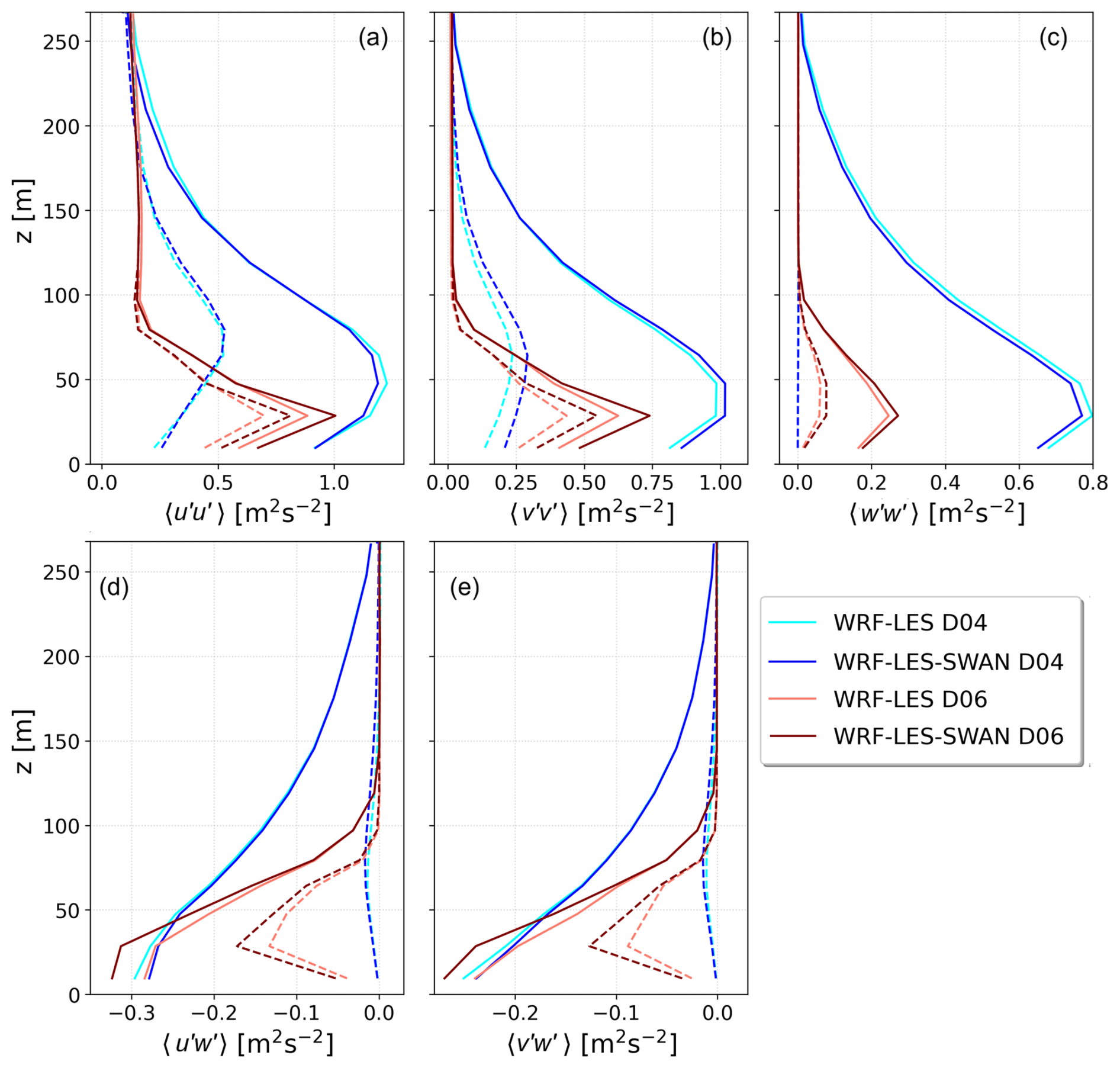
Figure 7 Vertical profiles of velocity variances (a) $\langle u^{\prime }{u}^{\prime }\rangle$, (b) $\langle v^{\prime }{v}^{\prime }\rangle$, and (c) $\langle w^{\prime }{w}^{\prime }\rangle$ and covariances (d) $\langle u^{\prime }{w}^{\prime }\rangle$ and (e) $\langle v^{\prime }{w}^{\prime }\rangle$ from WRF-LES and WRF-LES–SWAN runs at 100 m (D04) and 4 m (D06) horizontal grid spacings. Dashed and solid lines represent resolved and total (resolved + SGS) fluxes, respectively.

As no turbulence measurements are available from the RUNE campaign, these differences in turbulence should be interpreted as physics-based model behavior rather than validated improvement. It is also important to mention that all domains share the same spin-up period, and despite the shorter total runtime of D05 and D06, the turbulence fields in these fine LES nests are well developed, as indicated by the larger resolved variances relative to D04. The shorter runtime primarily limits the length of the available time series rather than the development of turbulence. The D05 and D06 domains are therefore included to illustrate how increasing horizontal resolution modifies the balance between resolved and SGS turbulence and to highlight the limitations of the 100 m LES configuration (D04) in representing near-surface turbulent structures. Consistent with previous LES studies, finer grid spacing is expected to increase the fraction of explicitly resolved turbulence and improve the representation of turbulent statistics, although no direct observational data are available for validation in this case.

3.5 The impact of cell perturbation method

Figure 8 shows the 24 h time series of wind speed at 40 m from the nested LES domain (D04), with and without CPM. The results highlight the role of CPM in enhancing wind speed variability and fluctuations.

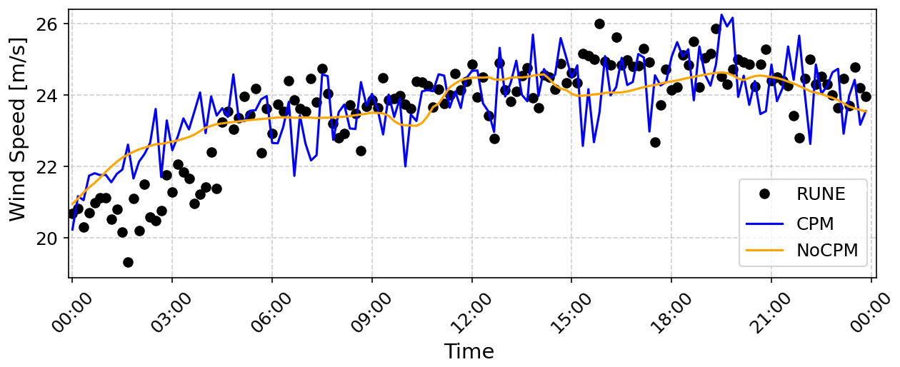
Figure 8 10 min time series of wind speed at 100 m from the D04 simulation, with and without activating the CPM, compared to that from measurements, over the period 00:00 to 23:59 UTC.

To further detail the enhancement of turbulence by using CPM, we compute in Fig. 9 the wind speed spectrum from lidar measurements, the finest mesoscale domain D03, and the nested LES domain D04, both with and without CPM. The spectrum is an average of spectra derived within 5 h windows with a 15 min overlap. As illustrated, the spectrum from the no-CPM case fails to capture the levels of turbulent energy in the measurements even at timescales much larger than 10 min and closely resembles the mesoscale spectrum, which is not expected to resolve turbulence. In contrast, the D04 simulation with CPM activated matches the spectral energy distribution of the measurements more closely. The drop in energy at higher frequencies of the spectrum for WRF-LES with CPM can be noticed beyond the timescale of 1 min, which shows the limitation of coarse LES runs to properly reproduce a wide range of turbulence scales.

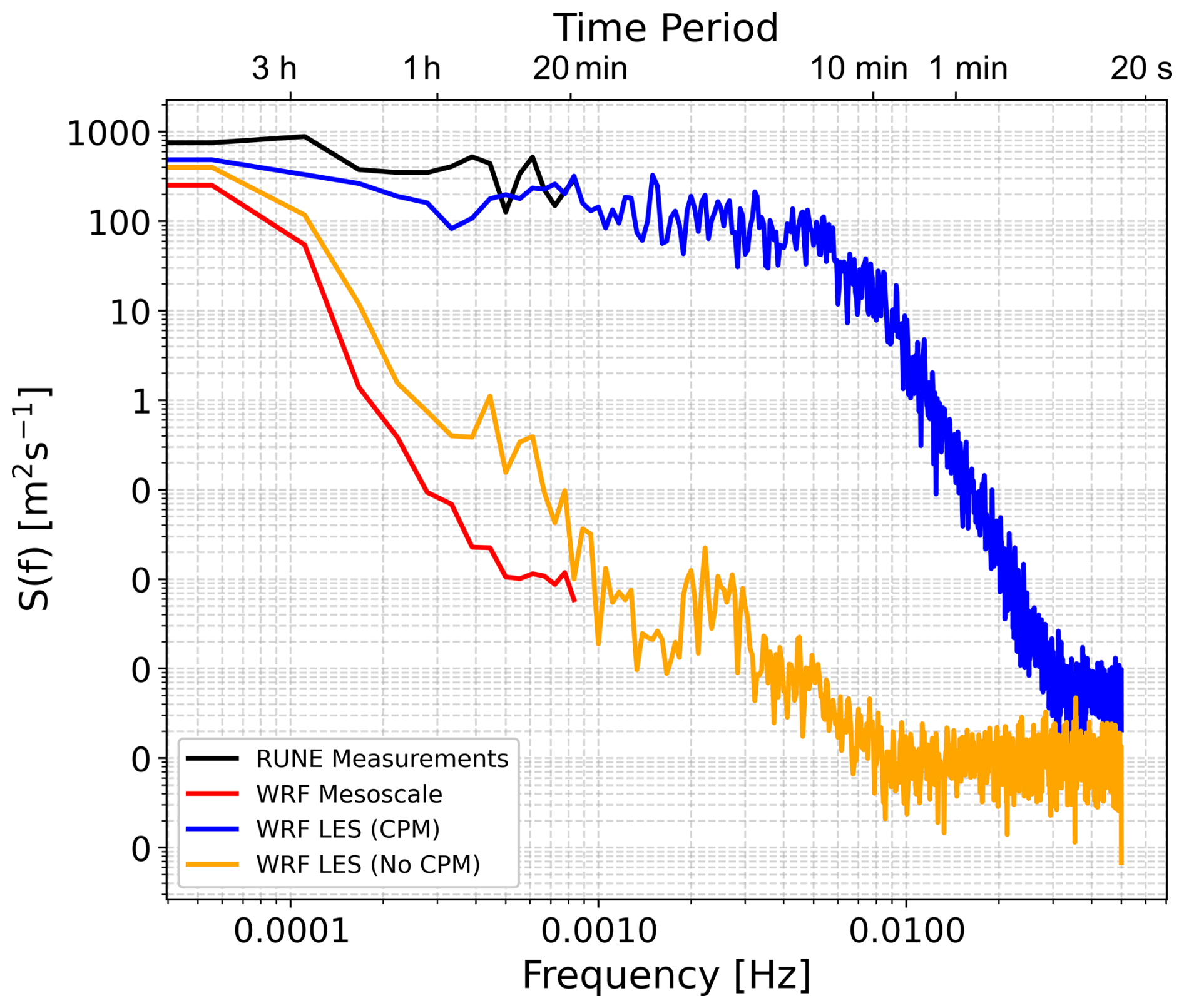
Figure 9 Spectrum of wind speed at 100 m from the mesoscale domain (D03), the LES domain (D04) both with and without CPM, and the RUNE measurements.

4 Discussion

We successfully coupled the WRF model in LES mode with the SWAN wave model within the COAWST system. This allows an examination of the air–sea interaction at high spatial and temporal resolution within the coupled model system. We tested this new system with a case study, which is a storm event in the North Sea, previously studied in Hamzeloo et al. (2025). Following the latter study, we chose this day due to the availability of measurements, for both the atmosphere and waves, and because it is a 1-year return event, which is relevant for offshore wind and wave operational purposes. In addition, the wave age $c_{\mathrm{p}}/U_{\mathrm{10}}<\mathrm{1.2}$ (c_p is wave phase speed) during the simulated period suggests that the dominating waves are young and growing. Thus, it is a relatively easy case to start with testing our new coupled modeling system.

The comparison between coupled and uncoupled LES runs shows that wave–atmosphere interactions have a measurable impact on both mean flow and turbulence characteristics. The improvement in the significant wave height and mean wind speed up to 100 m when using the coupled WRF-LES–SWAN model indicates the importance of the online coupling, as their feedback modifies the exchanges in the WBL. This is mainly due to improvements in surface roughness and momentum flux estimations, which impact the wind field near the ocean surface. However, the relatively small differences in mean wave direction and peak wave period show that not all wave parameters are equally sensitive to the coupling, and the benefits may depend on the specific conditions of the event. The vertical wind profiles indicate that the better statistics on mean winds in Table 2 for the LES runs are achieved due to excessive vertical wind shear in LES near the surface, which is most probably caused by the SGS model. In contrast, the mesoscale simulations reproduce the vertical wind shear and veer close to that of the observations, although the LES runs capture greater variability in wind speed. The mesoscale simulations exhibit a positive bias at all vertical levels, which may be related to biases in the boundary conditions, while the LES shows a negative bias below approximately 90 m and a positive bias above this level.

Note also that the 1 d storm case, although ideal for an initial test of the new coupled modeling system, does not represent the wide range of sea states that the North Sea experiences. Often, the North Sea sea state is complex with the presence of both wind-generated waves and swell, with waves aligned or misaligned with the wind. Measurements suggest that the air–sea momentum exchange can be reduced or enhanced depending on the alignment of swell and wind sea; see analysis of high-frequency wind and wave measurements in, e.g., Larsén et al. (2003). The effect of non-local swell and its misalignment with the wind sea has been previously implemented in different wave models in, e.g., Wu et al. (2016) and Porchetta et al. (2019). Swell can also develop locally from the wind sea; with a varying wind field with changing wind direction, it can be mixed together with the waves generated locally, resulting in misalignment. The current modeling system using WBLM includes the swell developed locally and hence the associated misalignment; this was previously analyzed in Fischereit et al. (2022). It is in our interest in the future to examine how our modeling system performs and potentially how to improve its performance in such complicated sea states.

The analysis shows that the coupled simulation produces higher horizontal and vertical velocity variances, which suggests enhanced turbulent mixing. This finding is consistent with theoretical expectations (Sullivan et al., 2008) and our previous modeling efforts (Hamzeloo et al., 2025). Due to the absence of direct turbulence measurements at the RUNE site, we are not able to quantify the accuracy of the turbulence simulations. At the beginning of our analysis, we examine the results from domain D04 with a horizontal grid spacing of 100 m. In this configuration, the vertical distribution of turbulence fluxes shows the largest value at 70 m height and unrealistically small vertical velocity variances. For finer horizontal grid spacings, Δx=20 m, the largest turbulence fluxes were present at slightly lower heights. With further refinement, Δx=4 m, the largest turbulence fluxes are at a height of around 25 m, and the vertical velocity variance reached more realistic magnitudes. The analysis confirms that fine horizontal grid spacing is essential for capturing the turbulence characteristics close to the surface and within a significant portion of the MABL. This is in agreement with the results in Sanchez-Gomez et al. (2025), who performed a multiscale simulation with two nested LES domains around Hurricane Laura, using horizontal grid spacings of 33.33 and 11.11 m. They found that the coarsest simulation could not resolve turbulence close to the surface, while the finer resolution matched the turbulence statistics of the measurements.

Furthermore, two distinct processes contribute to the observed differences in turbulence parameters in Fig. 7. The increase in wind speed variability from D03 to D04 arises from the change in turbulence representation when moving from a mesoscale PBL scheme to the LES SGS model, combined with the resolution dependence of the resolved–SGS partition at 100 m. In contrast, the differences between the coupled and uncoupled simulations within the same domain represent the physical impact of wind–wave coupling: the WBLM modifies the effective roughness and contributes to the near-surface stress, thereby driving the observed changes in shear production (Fig. 6) and, therefore, an increase in turbulence intensity. However, it should be noted that at a 100 m resolution, a substantial fraction of the turbulence is still represented by the SGS model. Therefore, instead of reflecting changes in fully resolved eddies, part of the coupling response may simply be the SGS model adapting to the modified surface roughness. The finer LES domains (D05 and D06) further illustrate that increasing horizontal resolution increases the fraction of turbulence explicitly resolved.

The grid spacing jump from D03 (1100 m) to D04 (100 m) is larger than typically recommended but was necessary to reach LES-permitting resolution while keeping the multiscale simulation computationally feasible. This choice also avoids the gray zone (300–1000 m), where neither a PBL scheme nor LES is appropriate (Arthur et al., 2025; Juliano et al., 2022; Chow et al., 2019). With sufficient fetch and the use of the CPM, turbulence develops in D04 despite the large ratio. The vertical-to-horizontal grid spacing ratio of about 10:1 in D04 is common in WRF mesoscale configurations, and it did not cause numerical instability here; however, for LES it can influence how much near-surface turbulence is explicitly resolved and increases reliance on SGS stresses. This further implies that some of the turbulence response in D04 should be interpreted in terms of SGS–resolved partitioning rather than purely resolved flow dynamics. This behavior is reflected in the turbulence profiles of D04 (Fig. 7).

Note that in our simulation using the COAWST modeling system, we only activated the atmospheric and wave models. It would be of great interest in the future to couple the ocean model as well; it is expected that with more frequent and accurate updates of sea surface temperature through the ocean model, some storm characteristics can be improved (Li and Tan, 2023). It is also expected that during storm conditions, water currents in certain areas, e.g., shallow water regions, would also affect the air–sea interaction. Although this feedback may affect wave development and near-surface stability in shallow shelf regions, our previous analysis of this storm showed that the event behaved as a deep-water wave case based on the Forristall (2000) curve, suggesting that depth-related effects were limited during this particular case (Hamzeloo et al., 2025).

It is important to note, however, that SWAN is a phase-averaged wave model and does not resolve wave phases, even though the WRF-LES grid spacing is comparable to the wave wavelength. In the coupled system, waves affect the atmosphere only through phase-averaged quantities such as roughness length and surface stress. Therefore, the LES represents flow over a sea-state-dependent rough surface, not over phase-resolved moving waves. Wave-coherent effects are also not captured, which is a limitation of this approach.

In addition, we evaluate the impact of the CPM on the LES domain boundaries, which is applied for the first time in the WRF-LES model through the COAWST framework. In the simulation without CPM, the LES domain cannot sustain turbulence, and the results are similar to those of the mesoscale domain. More importantly, the ensemble-averaged wind speed spectrum indicates that the LES without CPM fails to capture the expected turbulence energy levels, even at timescales larger than those of 3D turbulence. In contrast, LES with CPM produces more realistic spectral energy distributions within a wider range of scales, consistent with previous real-time simulation studies (Peña and Mirocha, 2024).

While turbulence development in nested LES can in general be influenced by limited fetch and boundary conditions, in the present study the relatively large domain extent and the use of the CPM at the lateral boundaries promote rapid spin-up of resolved turbulence in the inner domains. Nevertheless, the results from the finest-resolution domains D05 and D06 should be interpreted qualitatively as a sensitivity test on the spatial grid spacing.

5 Conclusions

In this study, we coupled the WRF-LES model with the SWAN model within the framework of COAWST. We applied the coupled, multiscale modeling system to a real storm case and evaluated the model performance in capturing mean wind and turbulence characteristics within the MABL.

Both coupled and uncoupled LES results showed better agreement with measurements at heights closer to the surface due to excessive vertical wind shear reproduced within the LES domain. Compared to the standalone WRF or WRF-LES simulations, coupling does not show significant differences in the mean wind speed for this storm case, while it enhances the turbulence fluxes due to wave-modified surface roughness and pressure, although such enhancement could not be evaluated due to the absence of turbulence measurements. Turbulence in the layers close to the surface has been shown to be very sensitive to horizontal grid spacing. However, since the conclusions are based on a single storm event, and no direct turbulence measurements are available, it remains unclear whether the simulated changes in turbulence fields correspond to a more accurate representation of the marine atmospheric boundary layer. This study also shows that turbulence instigation (through CPM) is essential for reproducing realistic turbulence in LES domains over the sea.

For future work, we plan to perform multiscale simulations at a site where high-frequency turbulence measurements are available for in-depth analysis of turbulence characteristics. This will allow direct validation of simulated turbulence fluxes and help quantify the strengths and limitations of coupled WRF–LES–SWAN configurations under different wind–wave conditions. In addition, future studies should also investigate periods with different sea states, such as wind–wave misalignment and swell conditions, as well as the impact of modeled ocean dynamics through ROMS in the COAWST framework.

Appendix A: List of abbreviations

Abbreviation	Definition
CCI	Climate Change Initiative
COAWST	Coupled Ocean Atmosphere Wave Sediment Transport
CORINE	Coordination of Information on the Environment
CPM	Cell perturbation method
DHI	Danish Hydraulic Institute
DTM	Digital terrain model
DTU	Technical University of Denmark
ECMWF	European Centre for Medium-Range Weather Forecasts
EMODnet	European Marine Observation and Data Network
ERA5	ECMWF Fifth-Generation Atmospheric Reanalysis
ESA	European Space Agency
Hmax	Maximum wave height
Hs	Significant wave height
JONSWAP	Joint North Sea Wave Project
LES	Large-eddy simulation
Lidar	Light detection and ranging
MABL	Marine Atmospheric Boundary Layer
MIKE 3 Wave FM	MIKE 3 Wave Flexible Mesh
MWD	Mean wave direction
MYJ	Mellor–Yamada–Janjic
MYNN	Mellor–Yamada–Nakanishi–Niino
OSTIA	Operational Sea Surface Temperature and Sea Ice Analysis
PALM	Parallelized large-eddy simulation model
PBL	Planetary boundary layer
QNSE	Quasi-normal scale elimination
RMSE	Root mean square error
ROMS	Regional Ocean Modeling System
RRTM	Rapid Radiative Transfer Model
RUNE	Reducing the Uncertainty of Nearshore Energy
SGS	Subgrid-scale
SWAN	Simulating WAves Nearshore
T02	Average zero-crossing period
TKE	Turbulent kinetic energy
Tp	Peak wave period
UTC	Coordinated Universal Time
WAM	Wave model
WBL	Wave boundary layer
WBLM	Wave boundary layer model
WRF	Weather Research and Forecasting
WSM6	WRF Single-Moment 6-class microphysics scheme
YSU	Yonsei University