
the Creative Commons Attribution 4.0 License.
the Creative Commons Attribution 4.0 License.
 | 16 Nov 2026
An in-depth observational and modeling analysis to explore long-range offshore wakes under different stability regimes

Jeffrey M. Freedman
Philippe Beaucage
Nick Robinson
Akila Gothandaraman
As wind energy areas continue to be built out worldwide, it is increasingly important to understand the implications of long-range wind farm wakes on wind energy generation. While gross capacity factors can be estimated, the impacts of upstream wind farm wakes on downstream energy production, especially under stable conditions, are largely unknown. A clear understanding of marine atmospheric boundary layer (MABL) stability in offshore regions is still evolving, as continuous high-resolution thermodynamic profiles in the MABL are uncommon. Given the relationship between stability and long-range (>50 km) offshore wakes, it is increasingly important to reliably estimate stability conditions in offshore regions. With the lack of consistent observations in and around offshore wind farms, it is necessary to rely on mesoscale models such as the Weather Research and Forecasting (WRF) modeling system to estimate stability and wake lengths. For this work we test WRF's ability to reproduce wake effects and potential losses using flight data over wind farms in the North Sea to evaluate its performance. As thermal stability is critical to understanding wake length, different metrics are evaluated to determine the best way to parameterize atmospheric stability from the WRF model. Results show that the bulk Richardson number derived from WRF can be used as a reliable metric to classify stability and that wake lengths are well represented under stable conditions.
- Article
(12355 KB) - Full-text XML
- BibTeX
- EndNote


It is widely accepted that offshore wind farm wakes can propagate downstream beyond 50 km under stable atmospheric conditions (Fitch et al., 2022; Platis et al., 2018; Cañadillas et al., 2020; Golbazi et al., 2022; Ali et al., 2023; Hahmann et al., 2025). While downwind wakes from wind turbines onshore have been extensively studied (Lundquist et al., 2019; Debnath et al., 2022; National Renewable Energy Laboratory, 2022; Krishnamurthy et al., 2025; Rogers, 2024), wind farm waking in the offshore meteorological–oceanographic (“met–ocean”) environment remains less understood. Understanding the frequency, extent, and deficits in wakes, and their relationship with offshore atmospheric stability, will help improve resource and energy yield assessment as well as wind farm production forecasting.
Wind farm wakes are a product of momentum sinks and turbulent kinetic energy (TKE) generation from large turbine arrays (Fitch et al., 2022; Golbazi et al., 2022; Hahmann et al., 2025) resulting in a downwind speed reduction and an increase in turbulence. Previous modeling studies performed over the United States East Coast have found a wind speed deficit, on average, of 2 m s−1 within a simulated wind farm and 0.5 m s−1 in the downwind wake (Golbazi et al., 2022). Although offshore wakes have been found to generally extend about 50 km downwind, very stable conditions may result in even longer wakes, potentially reaching distances of 100 km (Emeis, 2010; Fitch et al., 2022; Platis et al., 2018; Cañadillas et al., 2020; Golbazi et al., 2022; Ali et al., 2023; Hahmann et al., 2025). These wakes can be further amplified by wind direction based on the upwind fetch or wind direction alignment with the wind farm turbine rows (Platis et al., 2020; Hahmann et al., 2025).
Over land, wakes are generally shorter in distance as a higher surface roughness and more ambient turbulence allow them to dissipate more quickly (Platis et al., 2018; Pryor and Barthelmie, 2024). However, the ocean often features lesser turbulence due to a smoother surface and reduced thermal convection (Barthelmie, 1999; Hansen et al., 2012; Platis et al., 2018; Pryor and Barthelmie, 2024). A yearlong study in the offshore waters of Denmark (Barthelmie, 1999) found stable and near-neutral conditions occur 36 % and 53 % of the time, compared to only 11 % for unstable cases (Hahmann et al., 2025).
A major limitation to understanding how wind farm wakes behave offshore is a lack of measurements in areas within and directly downwind of wind farms. The North Sea offers a long duration of offshore wind deployment, beginning in 2001 with construction of Horns Rev 1, the first modern large-scale (160 MW) wind farm (Ørsted, 2019; Kihlström, 2023; Vattenfall, 2025). In situ measurements in the region include meteorological towers, Forschungsplattformen in Nord- und Ostsee (FINO) 1 and 3, which were unwaked prior to 2010 and 2014, respectively, but are now located within and alongside turbine arrays.
As a result of limited in situ measurements of offshore wakes, research of the downwind wake generally relies on SAR satellite imagery (Christiansen and Hasager, 2005, 2006; Hasager et al., 2015; Djath et al., 2018, 2022), operational turbine SCADA data (Foreman et al., 2024), or lidar data (Cañadillas et al., 2022). However, two flight campaigns in the late 2010s provided some of the first measurements of offshore wind farm downwind wakes. The WInd PArk Far Field (WIPAFF) campaign in 2016 and 2017 included a total of 41 research flights (Platis et al., 2018; Bärfuss et al., 2019) and X-Wakes collected data from an additional 49 flights in 2020 and 2021 (Rausch et al., 2023). Previous analysis of the WIPAFF measurements by Cañadillas et al. (2020) and Berge et al. (2024) found a phase error (i.e., a time shift between the modeled and observed evolution) when comparing these observations to mesoscale models, given that each flight occurs over a period of a few hours.
Current engineering wake models used in the wind industry, such as the DAWM-EV (Brower and Robinson, 2009) and TurbOPark (Nygaard et al., 2020; Pedersen et al., 2022), perform well at simulating internal wake losses; however, they do not include different atmospheric stability classes and thus they show faster wake recovery than is observed and are not able to capture wind speed deficits at downstream distances of 40–50 km (Fischereit et al., 2021, 2022; Stoelinga et al., 2022; Berge et al., 2024; Porchetta et al., 2026). Higher fidelity modeling is necessary to capture long-range wakes under non-neutral thermal conditions; however, large eddy simulations (LES) are computationally expensive when simulating large wind farms (Xia et al., 2017; Zhan et al., 2020). Therefore, recent studies have been relying on mesoscale numerical weather prediction (NWP) models such as the Weather Research and Forecasting (WRF) modeling system that are more practical for modeling large wind farms at regional scales (Xia et al., 2017; Fischereit et al., 2021; Stoelinga et al., 2022).
Long-range wakes can be modeled in the WRF model version 3.3 or later with the inclusion of the Fitch parameterization (Fitch et al., 2022; Archer et al., 2020; Skamarock et al., 2021) or the Ma–Archer–Vasel-Be-Hagh (MAV) scheme (new in WRF version 4.6.0; Ma et al., 2022). The limited availability of long-term data useful for analyzing offshore wind farm wakes necessitates reliance on atmospheric models with a full physics parameterization suite, such as WRF, to understand the offshore wind resource and variability and to predict wake losses (McCabe and Freedman, 2025). However, very few studies have been able to validate the accuracy of the WRF model for capturing wake losses, wake extent, and the relationship with stability in an offshore environment. Berge et al. (2024) was among the first to compare data from four flights during the X-Wakes campaign to WRF simulations. They found that WRF performed well in capturing wake losses, especially in proximity (20–30 km) of the farms. In this study, 41 flight cases from the WIPAFF experiment and long-term measurements at the FINO3 tower in the North Sea are used to validate WRFs ability to predict thermal stability and accurately simulate long-range (>50 km) offshore wakes.
This study provides the first in-depth analysis validating the WRF model-derived bulk Richardson number and capping inversion height to observations in offshore regions. The work done here is increasingly valuable, given the continued development of offshore wind worldwide. The findings in this study can be applied to other regions and help to establish a robust climatology of stability and to better understand conditions during which long-range wakes are most likely to occur.
This paper is organized as follows: data used to validate the WRF model are described in Sect. 2. Methods used in the analysis are discussed in Sect. 3. Section 4 uses the results from the WIPAFF flight experiments to compare against the WRF model. Section 5 uses the results of the model validation to better understand the meteorological environment in the North Sea. Summary and conclusions are discussed in Sect. 6.
2.1 WIPAFF flights
The WIPAFF campaign features the first offshore in situ measurements of the region downwind of large wind farms (Platis et al., 2018; Bärfuss et al., 2019). In 2016 and 2017 a Dornier DO 128 research aircraft flew 41 flights over wind farms in the German Bight (specifically focusing on wind farm grouping Amrumbank West, Nordsee Ost, and Meerwind Süd/Ost, as well as Gode Wind 1 and 2; Fig. 1a). Measurements used here include the aircraft's position (coordinates, altitude, aircraft velocity, roll, pitch, and heading using a combination of an inertial measurement unit [IMU] and GPS), wind speed and direction (estimated from the u, v, and w components), air temperature, relative humidity, density, and pressure at 100 Hz (Platis et al., 2018). Instruments used include a Rosemount 5-Hole-Probe (for wind components), Rosemount 1221 and 1201 pressure transducers, Rosemount temperature sensor (fast and slow), and a Meteolabor Dew Point Mirror (humidity; Corsmeier et al., 2001; Platis et al., 2018). Measurements of sea surface temperature were recorded through a lidar scanning system (Platis et al., 2018). Details on other instruments on the aircraft can be found in Corsmeier et al. (2001). Flights lasted 2–4 h, with the downwind flight pattern generally shorter (∼1 h; Platis et al., 2018). Aircraft speed was 66 m s−1 and the flight tracks were flown at hub height (approximately 95 or 120 m depending on wind farm cluster) perpendicular to the mean wind direction, up to 50 km directly downwind of the wind farm (Fig. 1). Of the 41 flights, only 25 cases measure the wake directly downstream of the turbine (such as shown in Fig. 1a); the other 16 flights flew above the turbine rotor plane. Data were collected at a sampling rate of 100 Hz, and averaged to 15 s (approximately every 1 km, chosen to match the 1 km spatial resolution in the WRF model output) for the purpose of this study. The beginning and end of each flight was removed, so the analysis did not consider the measurements when the aircraft was taking off, landing, or getting into position.
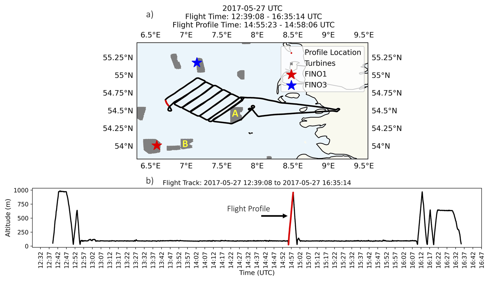
Figure 1(a) Flight plan on 27 May 2017 showing an entire flight track from take off to landing. Blue and red stars indicate the location of the FINO towers. Wind farms are represented by areas shaded in gray. Wind farm clusters composed of Amrumbank West, Nordsee Ost, and Meerwind Süd/Ost are shown by the letter A, and Gode Wind 1 and 2 by the letter B. (b) Time series of flight altitude (m) across entire flight track, with the red line showing the location of the atmospheric profile chosen for this flight.
In addition to the horizontal flight legs, the aircraft also measured atmospheric profiles through a steep ascent from approximately 50 to 1000 m a.m.s.l. (Fig. 1b; Platis et al., 2018). These profiles are averaged to 1 s, providing measurements at vertical height intervals ranging from 2 to 12 m. All flight profiles are taken away from land and outside of the waked region, so they are not directly impacted by wind farms (Fig. 1).
2.2 FINO towers
In situ offshore measurements have been collected at FINO1 since 2003, FINO2 since 2007, and FINO3 since 2009. Towers FINO1 and FINO3 are in the North Sea in proximity to the location of the WIPAFF flight campaign (Figs. 1a and 2). FINO2 is located further east in the Baltic Sea and is not relevant to this study. For brevity, results focus on FINO3 (55°11,7′ N, 007°9,5′ E). While FINO3 has been operational since 2009, after 2013 the tower was surrounded by operational wind farms (Sandbank and DanTysk). FINO3 measurements used include air temperature (at 29 and 95 m a.s.l.), relative humidity (29 and 95 m), pressure (23 and 95 m), and wind speed and direction (51, 71, and 91 m). The power law equation (see Eq. 1) is used to estimate wind speeds at 29 m a.m.s.l. from calculated wind speed shear between measurement heights 51 and 71 m a.m.s.l. (Eq. 2).
where α is the vertical speed shear, is the wind speed (m s−1), z is the height (m), and is the wind speed at a reference height, zr.
3.1 WRF model setup
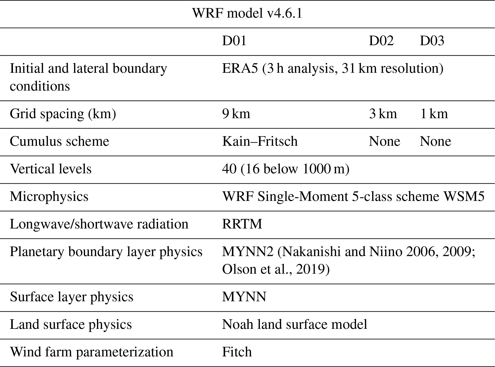
WRF model version 4.6.1 is used to conduct 36 h simulations, including a 12 h spin-up. The 27 simulations were centered over the North Sea region (Fig. 2; see days that were simulated in Table 4). The WRF model is initialized using ERA5, the fifth-generation ECMWF atmospheric reanalysis (European Centre for Medium-Range Weather Forecasts, 2019; Hersbach et al., 2020) and a one-way nested three-domain setup, with grid resolutions of 9, 3, and 1 km (Table 1). Wind farms are included in the model using the Fitch Wind Farm Parameterization (WFP; Fitch et al., 2022; Archer et al., 2020). The Fitch WFP is compatible with the MYNN2 (Nakanishi and Niino, 2006, 2009; Olson et al., 2019) PBL parameterization, with corrections suggested by Archer et al. (2020) incorporated into WRF model version 4.2.1 et seq. These corrections included a bug fix and a reduction in added turbulence kinetic energy (TKE) to be a quarter of the original value (Archer et al., 2020). Other model physics choices are shown in Table 1.
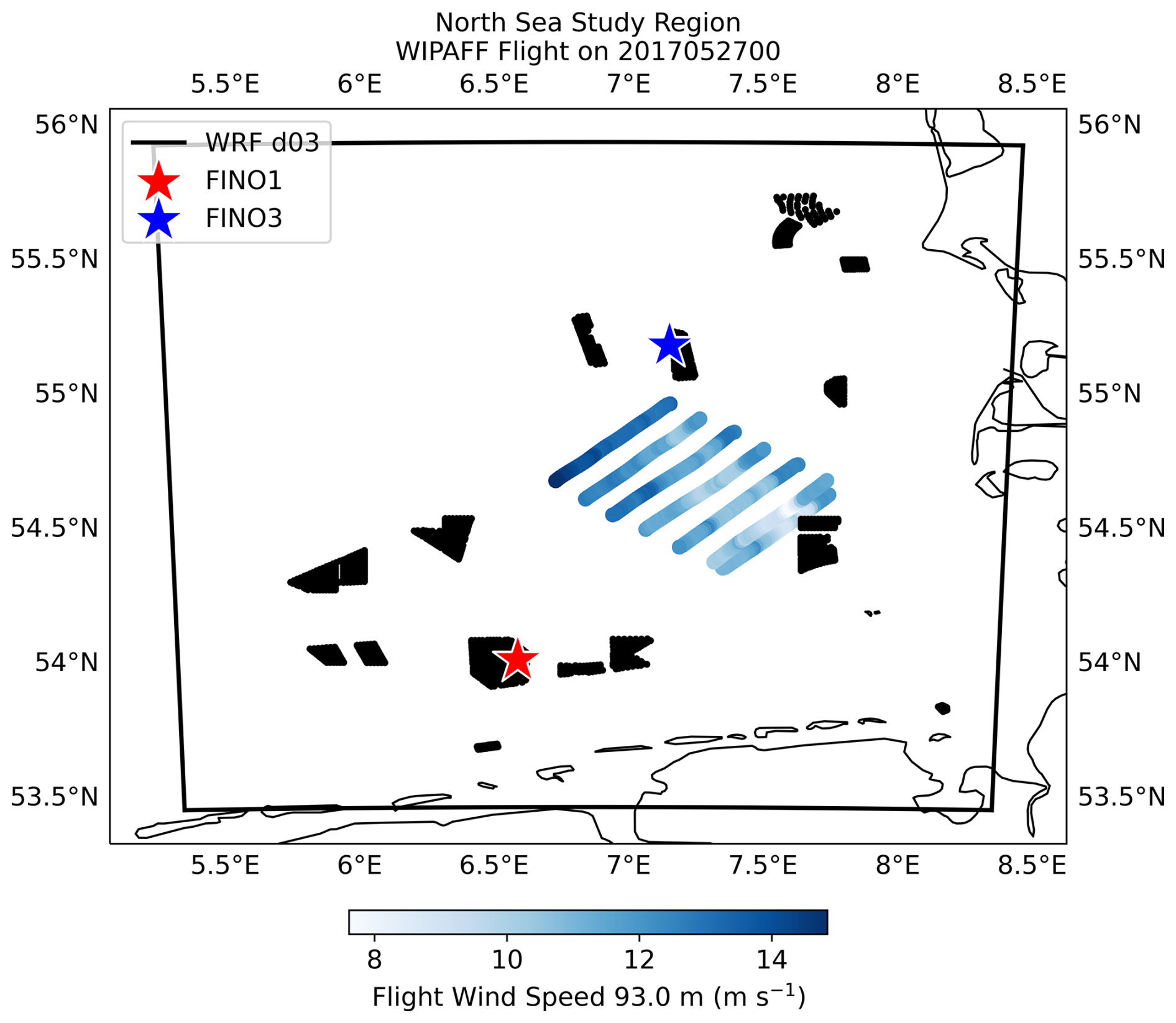
Figure 2WRF (version 4.6.1) inner domain (d03) extent over the North Sea. FINO towers 1 and 3 are shown by the red and blue stars. Location and wind speed (m s−1) of the WIPAFF flight on 27 May 2017 is also shown. Wind turbines used in the simulations are represented as black scatter points.
Model simulations are performed over the German Bight region of the North Sea, and analysis focuses on the innermost domain (D03; Fig. 2). Hub heights over the North Sea are 85–110 m a.m.s.l., and the turbines rated capacity ranges from 2 to 9 MW depending on the array. Turbine placement is set as the wind farms are already operational (Fig. 2; Nick Robinson, personal communication, October 2024). Both operational and planned wind farms outside of the inner domain region are not considered in this analysis.
3.2 Stability calculations
Different methods for estimating atmospheric stability from WRF are evaluated for this analysis. The Monin–Obukhov stability parameter, defined as the ratio of measurement height (z) to the Obukhov length (L), is commonly used to classify atmospheric stability (Monin and Obukhov, 1954; Barthelmie, 1999; Floors et al., 2011; Archer et al., 2016; Cantero et al., 2022; Rosencrans et al., 2024). However, because the observational dataset does not include in situ surface flux measurements, L cannot be derived from the observations and therefore this approach cannot be used for the observational analysis. We therefore consider stability metrics that allow for direct comparison between the stability derived from WRF and observations. These include the following.
-
The bulk Richardson number (Rib), an approximation of the gradient Richardson number, which estimates stability using local gradients of wind and virtual potential temperature (Eq. 3; Stull, 1988). The Rib considers turbulence generated both mechanically and buoyantly and is given by
where Δz represents the thickness (m) of the layer, θv is the mean layer virtual potential temperature (K), and ΔU and ΔV represent the gradient in the wind components of the layer (m s−1 m−1). As Rib (further referred to as the “bulk Ri formulation”), is an approximation, there are no universally established thresholds that define when the flow changes from stable to unstable (Stull, 1988). Mohan and Siddiqui (1998) use seven stability classes for Rib, and this has been used in recent studies (Olsen et al., 2017; Ruisi and Bossanyi, 2019). This compares with simpler classification schemes, such as the three-class scheme used in Pronk et al. (2022). Their bulk Ri formulation (see Table 2) is based on 188 h of data collected from a tall tower in a rural location in central Illinois (USA; Mohan and Siddiqui, 1998). Given that the performance of the bulk Ri formulation is poor when comparing observations to model output (see further discussion below), the Businger and Businger–Hicks formulation laid out in Mohan and Siddiqui (1998) are also considered (Table 2).
-
The gradient of θv, or lapse rate δ, is a simpler way to assess stability, as it only considers the change in θv over a specified layer. Note that the thickness of this layer (values for Δz) varies based on observational data heights available.
Here, Δz represents the thickness (m) of the layer and Δθv is the difference in θv (K) across the layer. This is a simple approximation for stability, and while it is generally assumed that negative values are unstable and positive values are stable, for the purpose of this study values of less than or equal to −0.01 K m−1 are unstable, greater than or equal to 0.01 K m−1 are stable, and anything between are neutral. This is a modification of the classes presented in Cañadillas et al. (2022) as the classes presented in that study were not sensitive enough to decipher between neutral and unstable/stable conditions.
-
The air–sea temperature difference (ΔTAir-SST) is the simplest approach, as it is often the most accessible approximation of atmospheric stability over water (it only requires surface measurements, which are generally more available in offshore regions). Generally, warm air over cold water indicates stable conditions, while cold air over warm water indicates unstable conditions. The ΔTAir-SST is defined as the difference between the surface air temperature (here 2 m is used) and the SST. Stability classes are defined in Table 3.
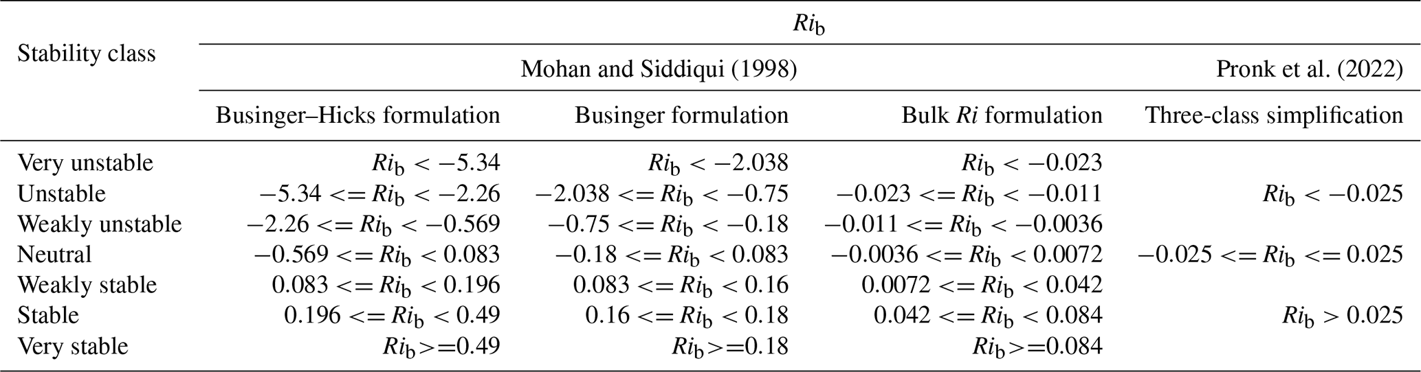
Table 3Stability classification thresholds for the ΔTAir-SST (K).

3.3 Capping inversion height
The capping inversion height (CIH) is defined as the height above the surface layer at which the potential temperature (θ) begins to increase, and a statically stable layer remains above, acting as the interface between the mixed layer and the free atmosphere (Stull, 1988). To determine the CIH, the strongest discontinuity in θ and specific humidity (q) within the lowest 1000 m are identified (Ball, 1960; Tennekes, 1973; Deardorff, 1979; Garstang and Fitzjarrald, 1999; Rampanelli and Zardi, 2004). Furthermore, the estimated inversion strength (EIS) is calculated using a method adapted from Wood and Bretherton (2006) and Wang et al. (2023).
To determine the CIH and EIS, the height of the strongest (positive) θ gradient is identified (Rampanelli and Zardi, 2004). As validation, the location of the strongest (negative) gradient in the q is also identified, as at the top of the mixed layer an increase in θ and a corresponding decrease in q are observed (Stull, 1988; Garstang and Fitzjarrald, 1999; McCabe and Freedman, 2025). To compare layers of equivalent thickness, all profiles, observed or modeled, are linearly interpolated to 30 m intervals. Given the profile limitations of the flight (only extending up to approximately 1000 m a.m.s.l.) the maximum gradient (in flight and WRF output) must occur within the lowest 1000 m. This ensures consistency in how the WRF and flight profiles are compared.
Using the maximum gradient as the baseline height, the EIS is then calculated across three levels (Wood and Bretherton, 2006; Wang et al., 2023).
-
Maximum gradient height and one level above
-
Maximum gradient height and two levels above
-
One level below maximum gradient height and one level above
The EIS is calculated between the three layers described above, using
where θ is the potential temperature at the top and bottom of the layer, and Γm is the moist adiabatic potential temperature gradient across the layer (Wang et al., 2023), given by
where Ra is the specific gas constant and cpa is the specific heat capacity for dry air at pressure (p), Lv is the latent heat and Rv is the specific gas constant for water vapor, and T is the air temperature. The moist adiabat is used as the inversion height is often close to saturation over the marine atmospheric boundary layer (MABL; Wang et al., 2023). Taking the largest value of the calculated EIS across the three layers, the CIH is determined to be the mean height of that layer (Wang et al., 2023). Note that if the EIS is <0.5 K, it is too weak to be considered an inversion and is disregarded, and the assumption is made that the CIH does not occur within the limitations of the profile.
To validate the WRF model's ability to properly represent stability regime and long-range wakes in an offshore environment, the WRF model is compared against the 41 WIPAFF flight cases. The study area focuses on the North Sea, specifically the German Bight region north and east of the German coast between approximately 5.5–8.5° E and 53.5–55.6° N (Fig. 2). Analysis time is presented in UTC (1 h behind local Central European Time (CET) and 2 h behind in summer, or CEST).
4.1 Flight analysis
Given the limited availability of measurements, few studies provide an in-depth observationally based assessment of the ability of the WRF-WFP to represent offshore long-range wind farm wakes in the context of atmospheric stability (Siedersleben et al., 2018). Using the WRF model to capture wind farm wakes is critical to reducing resource and forecast uncertainty given the global development of offshore wind. However, one problem with directly comparing flight data to the WRF model is the differences in temporal and spatial scales. WRF provides us with forecasts at a specific point in time (in this study, at 10 min intervals) with a spatial resolution of 1 km; however, the flights are taking point measurements at a frequency of 100 Hz over periods of a few hours (Fig. 1; Cañadillas et al., 2020; Berge et al., 2024).
Given the uncertainties in the spatial and temporal changes in wind speed that are inevitable with flight data, and the known timing phase error sometimes present in WRF (Cañadillas et al., 2022; Berge et al., 2024; McCabe and Freedman, 2025), to determine the proper time offset when comparing the WRF analysis to observations, the wind speed prediction along the flight track is compared to the WRF model forecast at various hourly intervals along the same path (Fig. 3). By identifying the nearest latitude/longitude coordinate to the flight observations and the closest time to the nearest 10 min WRF output file and by interpolating to the proper height (91 m a.m.s.l on 6 September 2016 and 94 m a.m.s.l on 27 May 2017), the modeled and observed wind speed are compared along the flight track (Figs. 3, 4, and 5). Following the method described in Berge et al. (2024), the WRF forecasts for up to 3 h prior and following the flight time is also considered to identify any time offsets. A time offset as large as +/− 5 h was considered for all cases, but wind speed phase errors were found to occur within a threshold of 3 h.
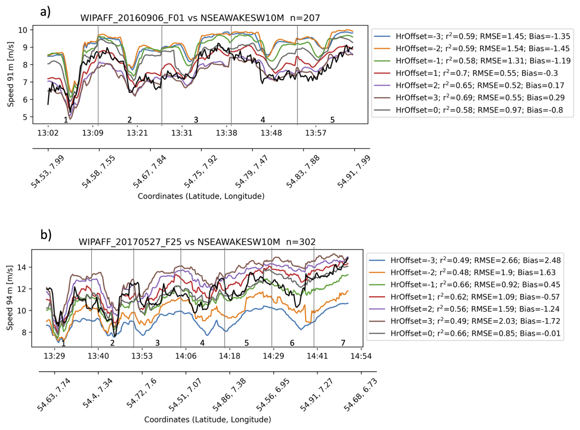
Figure 3Wind speed (m s−1) along horizontal flight legs (vertical gray lines represent each horizontal flight leg, numbered and shown in Figs. 4 and 5). Observed wind speed (black) is compared to WRF wind speed for different time offsets (+/−3 h) for (a) 6 September 2016 (see Fig. 5) and (b) 27 May 2017 (see Fig. 4).
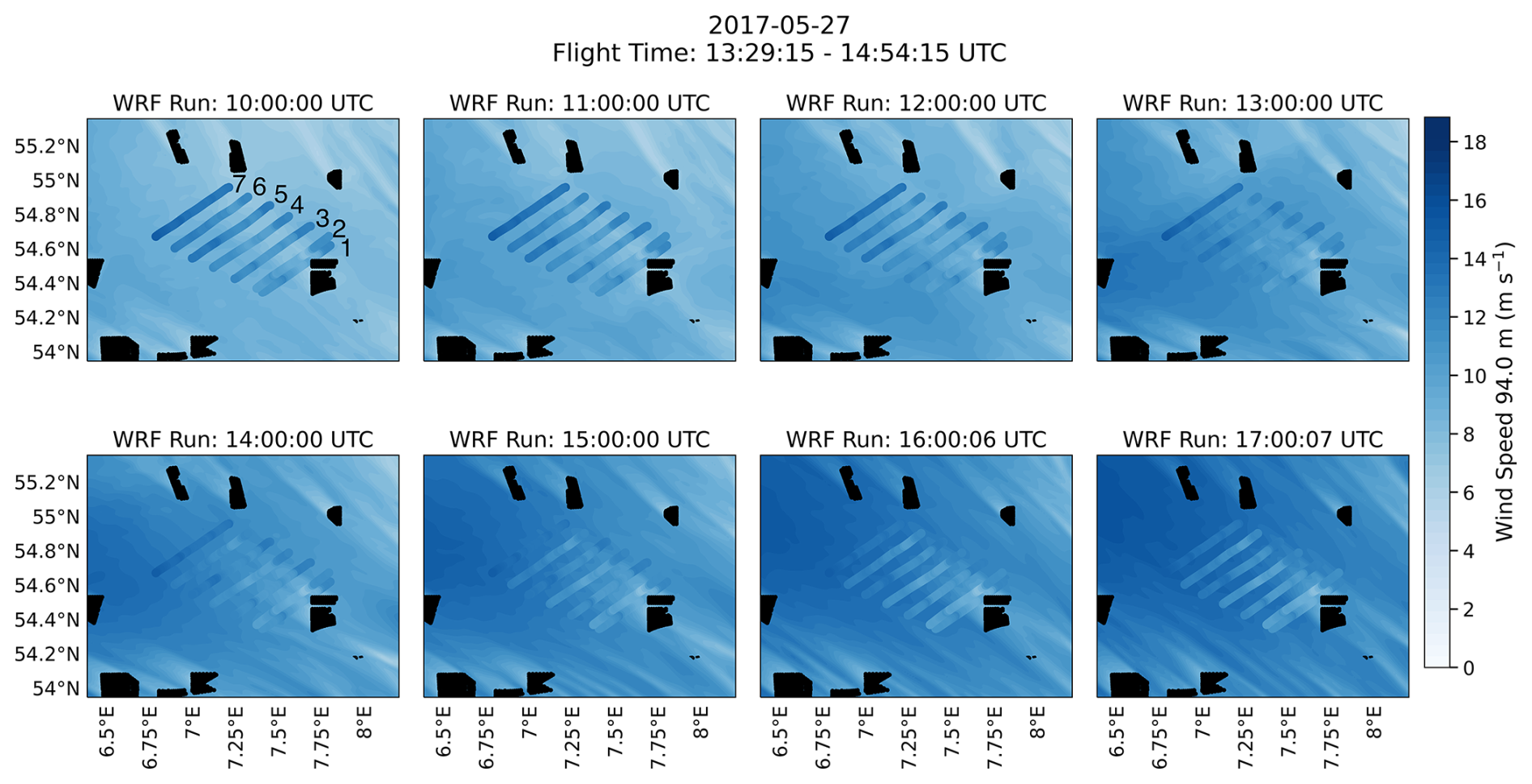
Figure 4WRF wind field on 27 May 2017 (contours) overlaid with wind speed (m s−1) measurements from WIPAFF flight (scatter points) for hours from 10:00 to 17:00 UTC. Black shaded areas represent wind farm locations. Consecutive flight legs are numbered in the upper-left panel.
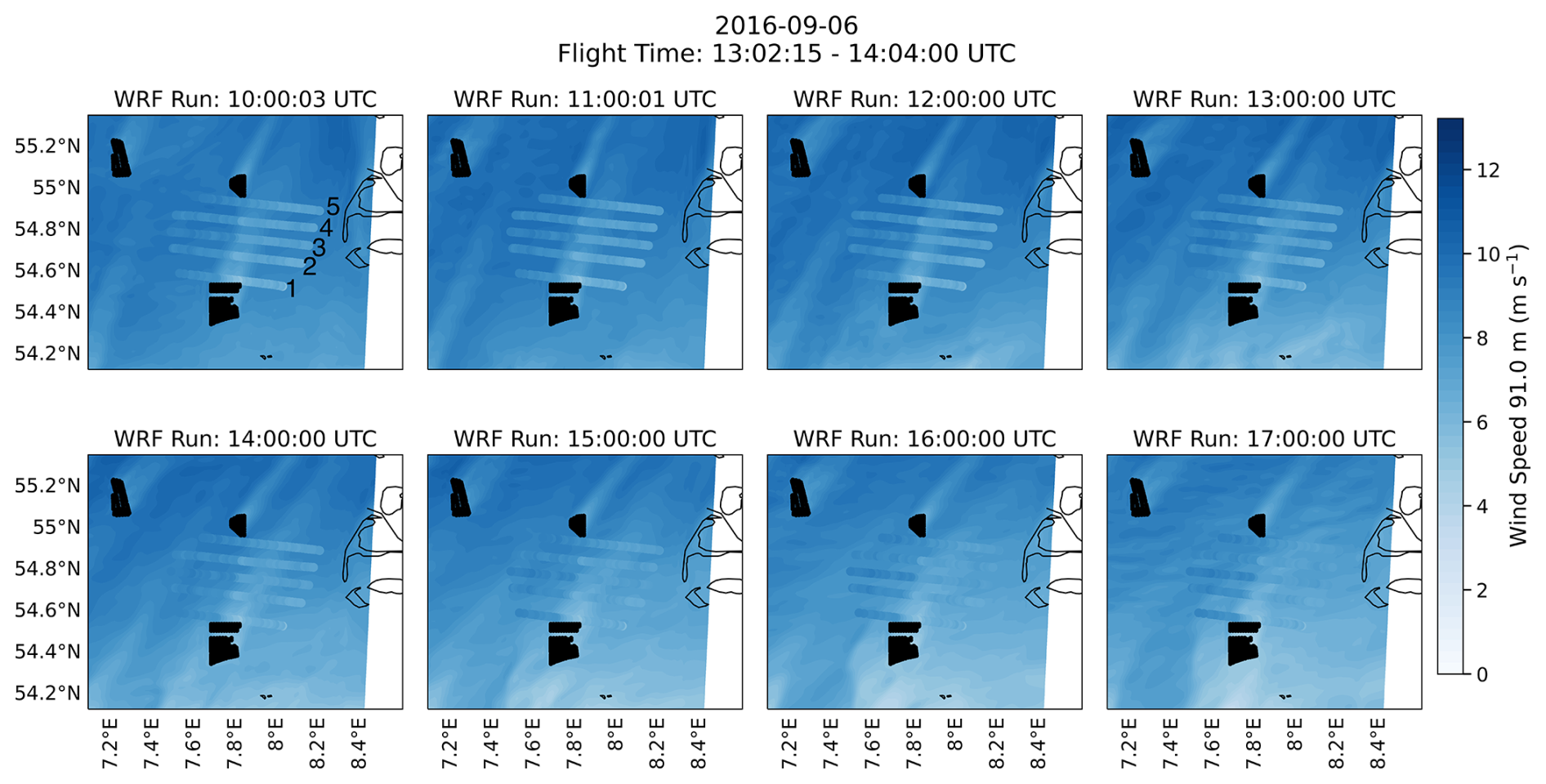
Figure 5Same as Fig. 4 but for 6 September 2016.
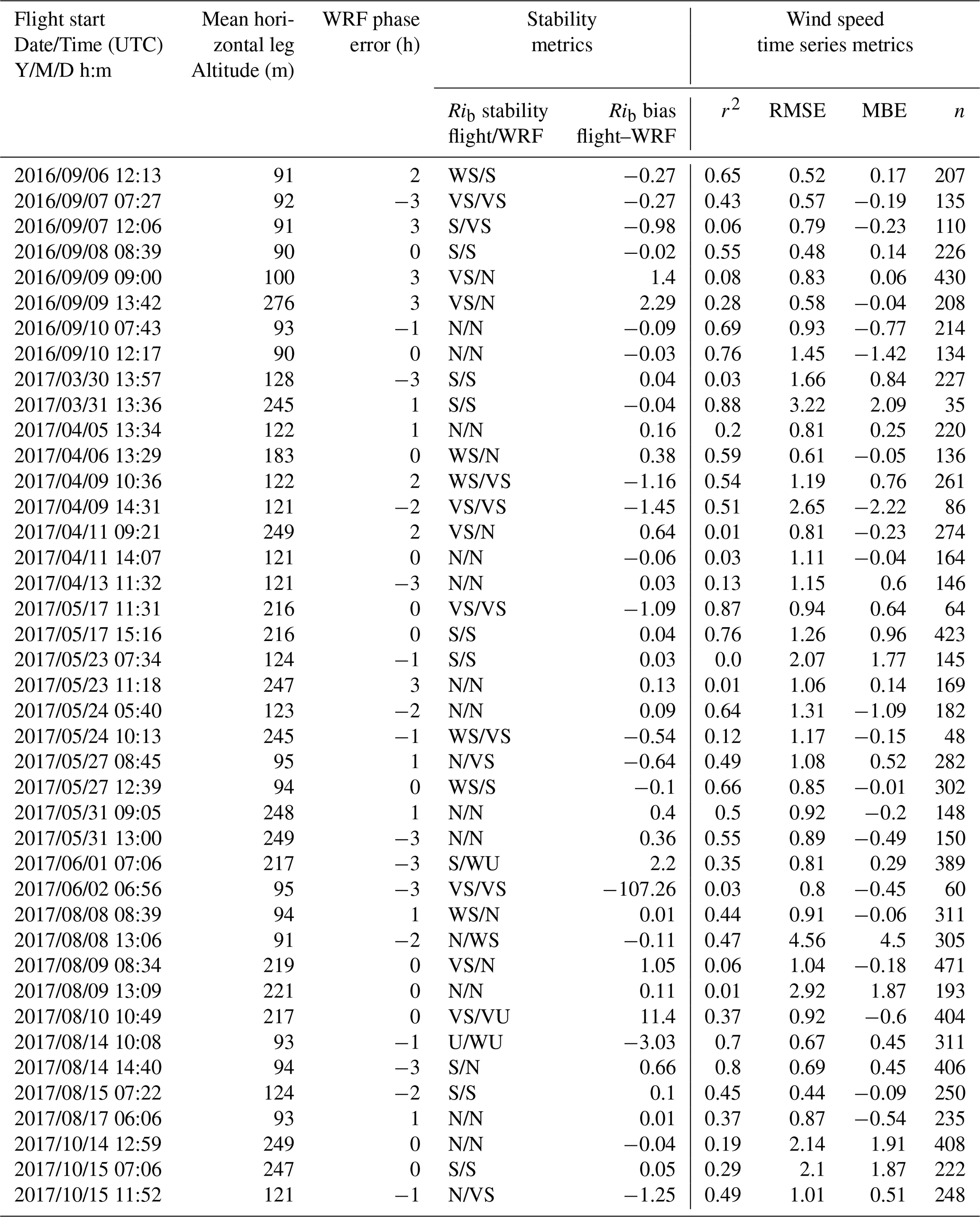
To account for a phase error in the analysis, various WRF forecast hours are compared with the flight observations using metrics including the coefficient of determination (r2), root mean square error (RMSE), and the mean bias error (MBE). The hour offset with the best combination of a high r2, low RMSE, and low MBE is determined to be the WRF phase error for that case. While all three metrics do not always agree, the MBE and RMSE are weighted higher than the r2. This decision follows the discussion in McCabe and Freedman (2025), noting that r2 has limitations in time series analysis to determining overall agreement between model results and observations. For example, the time offset used in the analyses for 27 May 2017 and 6 September 2016 is 0 and +2, respectively (Fig. 3 and Table 4).
Table 4Columns (left to right) show the flight start time (UTC), the mean aircraft altitude (m) along the selected flight path, the determined WRF phase error (hours), stability metrics including the stability classification from the flight and WRF profile for each case, calculated using the Businger–Hicks formulation. VS = very stable, S = stable, WS = weakly stable, N = neutral, WU = weakly unstable, U = unstable, and VU = very unstable. Rib bias (flight–WRF) is also shown. Lastly, wind speed metrics including r2, RMSE, MBE, and n (number of points compared) are calculated between the flight and WRF along the flight track (such as shown in Fig. 3).
To visualize the general performance of the WRF model in terms of the presence of a timing phase error, the flight-measured wind speed is overlaid with the WRF-predicted wind field. For example, on 27 May 2017, the flight duration of the cross-wake horizontal legs (Fig. 3) spanned just under 1.5 h, from 13:29 to 14:54 UTC. In addition to overlaying the WRF wind field for the hours concurrent with the flight (e.g., 13:00 and 14:00 UTC), the WRF wind speed prediction is again considered for the 3 h before and after the flight time. This allows for a qualitative understanding of overall WRF model performance in capturing the wake and the wind field change over the duration of the flight. On 27 May 2017, WRF performance is best in the hours coinciding with the flight, with a slight overprediction in the wind speed outside of the wake (Fig. 4). That said, WRF does well in representing the area of the largest wind speed deficit and the approximate length of the wake (Fig. 4).
For the 6 September 2016 flight WRF performs well in modeling the approximate length and region of the largest wind speed deficit. However, a phase error is noted on 6 September 2016, as 16:00 and 17:00 UTC, the hours directly after those concurrent with the flight time, best represent the measured wind field (Figs. 3a and 5). This method was repeated for all 41 WIPAFF flights, and the WRF hour offsets used in the analysis for all cases are shown in Table 4.
Other variables along the flight path, such as wind direction, temperature, specific humidity, and pressure, show good overall WRF performance (Fig. 6). Air pressure and specific humidity (although slightly higher in the observations on southeast side of the wake) show strong agreement between the observations and model. The small cross-wake differences in specific humidity are expected because the aircraft samples continuously along a moving flight path, whereas WRF represents grid-cell-averaged conditions. There is a cold bias (2–3 °C) in the WRF model-predicted air temperature, which is consistent across all 41 cases. García-Díez et al. (2013) also found a cold bias all over Europe varying by season and time-of-day when relying on the MYJ PBL scheme. These slight biases, however, can be meaningful when considering factors such as wake path or atmospheric stability. Any model output error is especially important when considering the potential effects on a downstream wind farm; e.g., a slight error in wind direction can significantly impact the forecasted wind resource at the downwind farm.
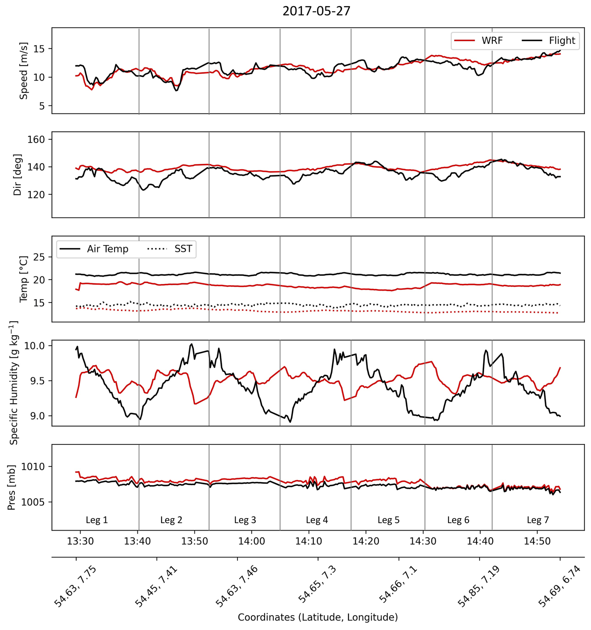
Figure 6Time series of variables along the flight track at 94 m a.m.s.l. From top to bottom: wind speed (m s−1), wind direction (°), air temperature (°C) and SST (dashed line), q (g kg−1), and air pressure (mb) for flight observations (black) and corresponding WRF predictions (red). Vertical gray lines represent each horizontal flight leg, numbered 1–7, and are shown along the flight path in Fig. 4.
For example, on 27 May 2017, the wind direction bias is small (error ranges from 13.3 to −3.9; Fig. 6); however, the WRF wind direction is slightly more out of the south, contributing to a bias in the wake location (e.g., the difference between the black scatter points and the gray line as shown in Fig. 7a). WRF predicts the wake to be slightly offset towards the north than is observed from the aircraft (Fig. 7a). In most cases this will not impact wake length or deficit predictions, but it may change the alignment with another downwind farm. This is important, as depending on the wind array, properly modeling wind direction and alignment of wakes with downwind wind farms is crucial to accurate energy modeling. A long downwind wake is also observed during this event, as it takes 57 km before the wake recovers to the wind speed of the no-turbine (control) WRF run (Fig. 7). The results are consistent with the observations (Fig. 7b) and with Cañadillas et al. (2020), who noted that wakes in the North Sea are found to extend over 50 km during stable conditions (Fig. 7b). On 27 May 2017, Cañadillas et al. (2020) notes the observed 95 % wake recovery length is 50 km compared to 40 km as shown in this WRF simulation (Fig. 7). This is confirmed by the observed 95 % recovery wake length of 40 km on 6 September 2016 (Cañadillas et al., 2020) to WRF's value of 32 km (not shown). This introduces two questions: (1) is the WRF model able to properly estimate atmospheric stability offshore and (2) is there a clear relationship between wake length and stability?

Figure 7(a) Contour plot of WRF 94 m wind field overlaid with flight wind speed measurements (m s−1; approximate hub height, 94 m) for 27 May 2017 at 14 UTC (WRF) and 14:29–14:54 UTC (flight). Location of flight profile and stability calculations is shown by the black diamond. FINO3 tower location is shown in the gray square. Gray line indicates the downwind transect along the wake deficit. Black circle indicates a selected location 25 km upwind from the beginning of the transect (red star). Black scatter points downwind of the wind farm represent the downwind transect along the observed wind direction. (b) Wind speed along the wake transect for the no wind farm control run (blue) compared to the WRF run with wind farms (red) and the observed wind speed along the observed wind direction for each flight leg (black). (c) Wind speed profiles upwind and downwind of the wind farm, shown along the wake deficit transect comparing the no wind farm control run (blue) and run with wind farms (red). Horizontal gray line indicates approximate hub height, ∼94 m a.m.s.l.
4.2 Stability analysis
Although atmospheric stability has been found to be integral in determining wake length (Emeis, 2010; Siedersleben et al., 2018; Cañadillas et al., 2020; Ali et al., 2023; Hahmann et al., 2025), few studies have utilized observations to determine the ability of the WRF model to capture the near-surface stability offshore. Atmospheric profiles measured by the aircraft across the 41 WIPAFF case studies provide valuable measurements of the wind and thermodynamic profile offshore and provide us with a high spatial resolution of vertical measurements. Without aircraft flux measurements, L cannot be directly derived from observations and thus does not permit a direct comparison with WRF model output. The ΔTAir-SST method is also inapplicable, as the measurements from the aircraft do not provide an ambient air temperature close enough to the surface (e.g., 2 or 10 m). Therefore, we focus on calculations of Rib and δ (Eqs. 3 and 4).
Considering three different stability classifications for Rib (see Table 2) the Businger–Hicks formulation results in a matching stability classification between the aircraft observations and corresponding WRF output more than 73 % (Table 4) of the time, compared to 70 % and 47 % when using the Businger and bulk Ri formulations. A stability match is considered when the stability classification agrees within one stability class, e.g., very stable and stable or near-stable and neutral. The Businger–Hicks formulation has the largest thresholds among different stability classes, making it less sensitive to small fluctuations in calculated Rib (Table 2).
Given the potential spatiotemporal biases in the flight profile, WRF's stability is also compared to measurements at the FINO3 tower. Note that in 2016 and 2017 the FINO3 tower, located adjacent to the DanTysk wind farm, provides in situ 10 min measurements of stability. From the flight data, stability is calculated between the lowest flight measurement and 100 m a.m.s.l. The lowest aircraft profile measurement varies depending on the flight, ranging from 14 to 86 m a.m.s.l., with an average profile start altitude of 44 m. Stability at the FINO3 tower is calculated between fixed measurement heights, 29 and 95 m a.m.s.l. WRF stability is calculated using the nearest available levels at the nearest grid point to both the location of the flight profile and FINO3 tower. For example, on 27 May 2017, stability at the flight profile location (Fig. 1) is calculated over a layer from 36 to 95 m a.m.s.l. and from 29 to 95 m at the FINO3 tower location. As shown, the profiles of wind speed, direction, and θ compare well with the concurrent WRF profile (Fig. 8). WRF underestimates wind speed and θ slightly; however, the shape and the stability of the profile is well represented (Fig. 8). When calculating Rib, the vertical gradients of wind speed and θ are most important (Eq. 3) and are shown to be better represented by the model when using thicker layers, such as the 36–102 m layer shown in this analysis (Fig. 8). However, when considering vertical gradients between each measurement height, the flight observations show stronger vertical gradients in wind speed, most apparent on 27 May 2017 at higher levels (>100 m), resulting in WRF overestimating stability in this layer (Fig. 8).
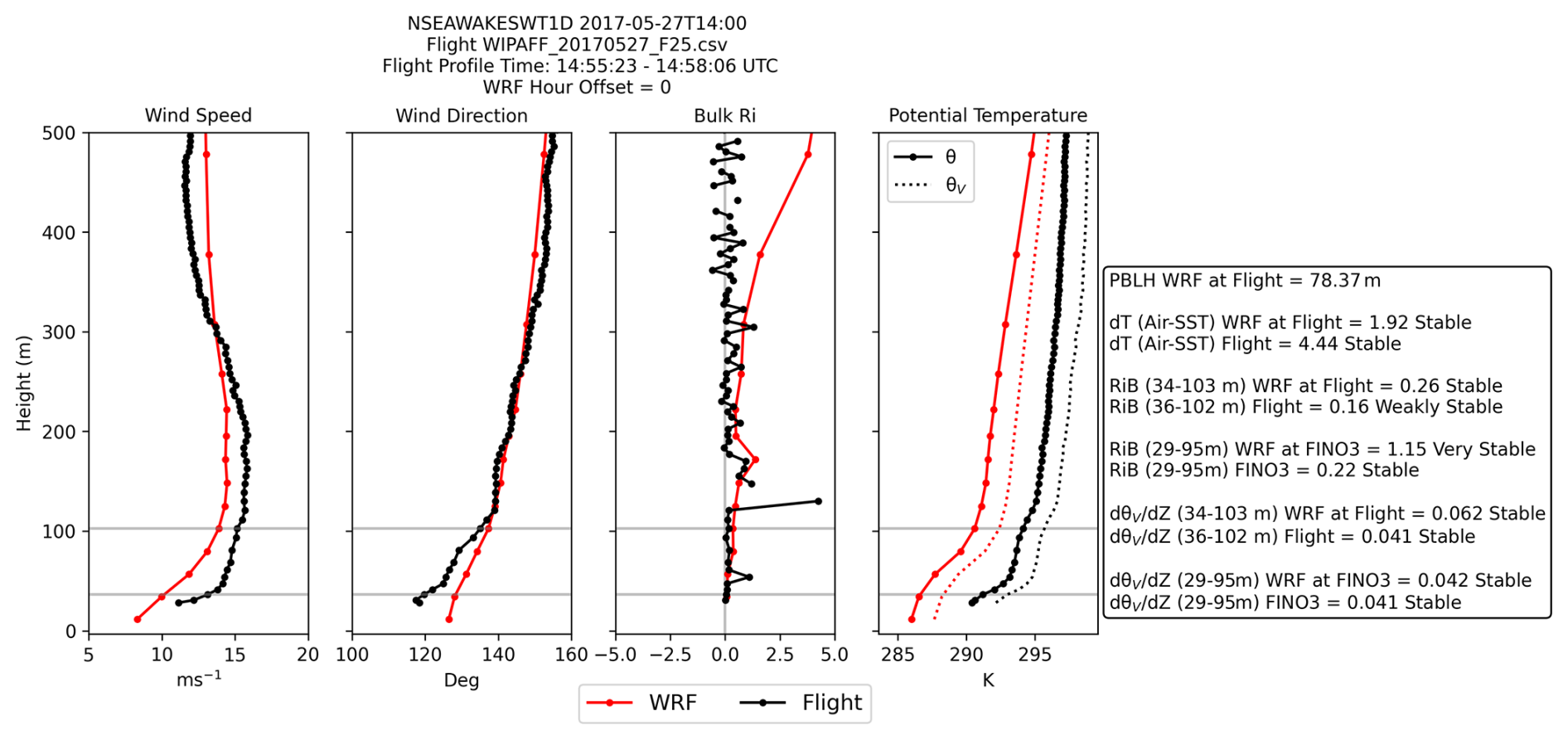
Figure 8Profiles of wind speed (m s−1), wind direction (deg), Rib, and θ (solid) and θv (dashed) for the flight observations (black) and corresponding WRF output (red). Metrics from WRF vs. flight profile location and FINO3 location are summarized in the text box on the right. Horizontal gray lines indicate levels of which metrics are calculated across.
As mentioned earlier, using the Businger–Hicks formulation to classify the Rib number into stability types indicates agreement between the WRF model and observations on 30 of the 41 flight cases. Classifying Rib into stability classes can be complicated, as results are dependent on the thresholds set for each stability class. For example, using the Businger–Hicks formulation gives a slightly different breakdown of stability across the 41 cases than applying the bulk Ri formulation (Table 2; Fig. 9a, b). However, overall, there is good agreement between the stability derived from the flights and the corresponding WRF runs (Table 4). Comparing the Rib and δ value at both the flight profiles and FINO3 tower to the corresponding WRF forecast shows that the 41 cases compare well on the sign of Rib and δ (positive vs. negative) and that all WIPAFF flights experience near-neutral to stable conditions (Fig. 9).

Figure 9Scatterplot comparing (a, b) Rib and (c, d) δ from WRF (x axis) to the measurements at flight (y axis; a, c) or FINO3 tower (y axis; b, d). (a–b) Shaded areas represent the neutral threshold zone for the Businger–Hicks formulation (blue), bulk Ri formulation (orange), and Businger formulation (green). The 1-to-1 line is shown in gray. (c–d) Green line indicates stable threshold, red line indicates unstable threshold, and gray line indicates the 1-to-1 line.
Despite some inconsistencies in the Rib stability classification, specifically the Businger–Hicks formulation, it serves as the best and most reliable metric to calculate stability offshore. Using δ results tend to overestimate the number of neutral cases (Fig. 9c, d).
In addition to validating WRF atmospheric stability regimes with the observations, we also evaluate WRF's ability to capture the CIH. Using the methods described in Sect. 3.3, the CIH is calculated using the strongest gradients in the θ and q profiles. Using this method for all flight cases, it is found that under stable conditions, the CIH derived from WRF and from the observations compares well, regardless of whether θ or q is used to initially determine the height of the strongest gradient (Fig. 10). Given the presence of near-neutral and weakly stable cases, some outliers are expected, as when the vertical profile is well mixed, gradients of θ or q are small, and errors between the WRF and flight results may be more common (Fig. 10a, b).
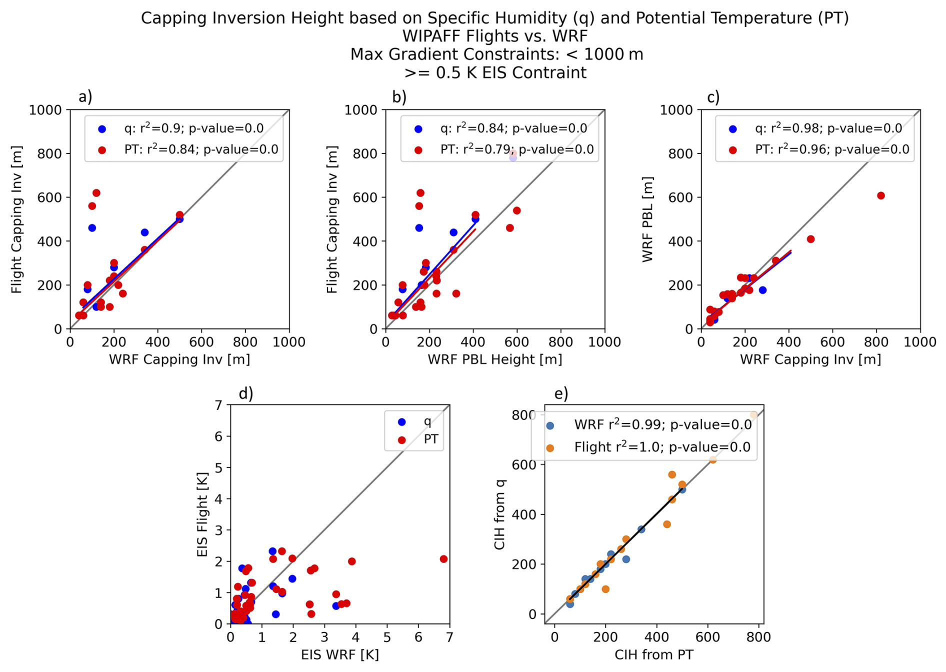
Figure 10Regression analysis for WIPAFF profiles of (a) flight capping inversion to WRF capping inversion, (b) flight capping inversion compared to WRF PBL height, (c) WRF PBL height compared to the WRF capping inversion, and (d) EIS derived from flight compared to EIS derived from WRF, for q (blue) and θ (red). Lastly, (e) compares the CIH calculated from q with CIH calculated from θ for the flights (orange) and WRF (blue).
Profiles of q and θ shown (Fig. 11) for two flight cases illustrate these results. For example, 27 May 2017 is a stable case (Fig. 8) with a CIH of 60 m (Fig. 11b). During stable events the CIH often falls within the rotor plane (generally between 60 to 120 m a.m.s.l. in the North Sea) and directional shear within the profile (especially apparent in the aircraft data) is also observed (Fig. 11). For 6 September 2016, a neutral case, the profiles of q and θ from the flight and WRF model agree well, but there is not a definitive enough inversion within the profile to determine the CIH (Fig. 11a). Slight differences in the specific humidity profiles between the model results and observations are expected, as the aircraft profile was collected during a continuous ascent while the aircraft was moving horizontally, whereas the WRF profile represents conditions at the nearest model grid point. Additionally, the WRF model's coarser vertical resolution smooths sharp moisture gradients, particularly near the capping inversion. Despite these differences, WRF captures the overall shape of the profile and the location of the strongest gradient in specific humidity associated with the capping inversion. Based on analysis comparing the CIH derived from WRF to the model-estimated PBL height provided in the standard WRF output, the PBL height can be used as a good approximation of the CIH when it cannot be explicitly calculated (Figs. 10b–c and 11).
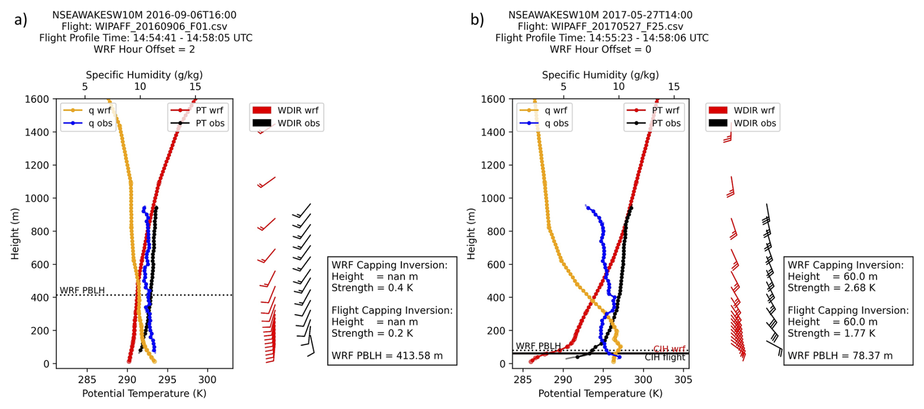
Figure 11(a) 6 September 2016 and (b) 27 May 2017. Profiles of θ (bottom x axis) from flight observations (black) compared to WRF (red) and profile of q (top x axis) for flight observations (blue) compared to WRF (yellow). Wind barbs (1 full barb = 5 m s−1) are shown for observations (black) and WRF (red). Also shown are the WRF PBL height (dashed black line) and the CIH from the flight (solid black line) and WRF (solid red line). Values for PBL height, CIH, and EIS are summarized in the text box to the right of the plot.
Following comparison of thermodynamic profiles between the WRF model and flight measurements and proving the reliability in metrics such as Rib derived from WRF model, Part 2 will discuss the overall climatological characteristics of the North Sea and how often stable conditions favoring long-range wake conditions may be expected.
We next consider the annual stability regimes of the North Sea in the context of long-range wind farm wakes. After demonstrating the validity of using the WRF model to derive atmospheric stability, the WRF model can be leveraged to gain a better understanding of the annual distribution of near-surface stability. To do so, a 4-year WRF time series (2010–2013) is run at the FINO3 tower in the North Sea (Fig. 2). Focus remains on the years 2010 through 2013, as this time period is prior to the development of nearby wind farms, including Butendiek, DanTysk, and Sandbank and includes concurrent FINO3 tower data. Model setup follows the WRF configuration described in Table 1. Note that for this analysis, WRF is run with WFP off.
While the annual wind speed variability is small, the directional variability is apparent in Fig. 12. Although the predominate wind direction is out of the western sector in all 4 years, 2010 features more northwest winds, while in 2011 the wind direction is commonly out of the west–southwest. This is confirmed by a change of 60° in the predominant wind direction between 2010 and 2011 (Fig. 12a–b). The annual mean SLP gradient for each year (not shown) shows 2010 to feature weaker gradients when compared to the other years (2011 and 2013 feature the strongest gradients). The WRF model captures this variability well, and accurately represents the wind rose when compared to observations. Note that FINO tower observations are not assimilated into the ERA5 reanalysis and therefore do not impact the WRF hindcasts (Hersbach et al., 2020).

Figure 12Annual composite wind roses for approximate hub height winds, 95 m, measured at the FINO3 tower for (a) 2010, (b) 2011, (c) 2012, and (d) 2013. The radial labels indicate the frequency (%) at which the wind blows from that direction.
In addition to variability in the annual wind direction, rather significant year-to-year changes in stability are noted. Stability is determined using the Businger–Hicks formulation for the Rib (Eq. 3; Table 2). Between 2011 and 2012 a shift is observed from more unstable to more stable conditions (Fig. 13a, b). Note the annual stability patterns in 2010 resemble 2011, with 2012 like 2013; therefore, only the years 2011 and 2012 are shown in Fig. 13. Interestingly, this shift is not seen by the concurrent WRF stability at the FINO3 tower location (Fig. 13c, d). However, both WRF and the FINO3 measurements indicate a high frequency of near-neutral conditions (Fig. 13). Some discrepancies may be introduced into the data by the choice of Rib stability classification, as the numeric thresholds of the stability classes are tightly binned (as shown in Table 2).
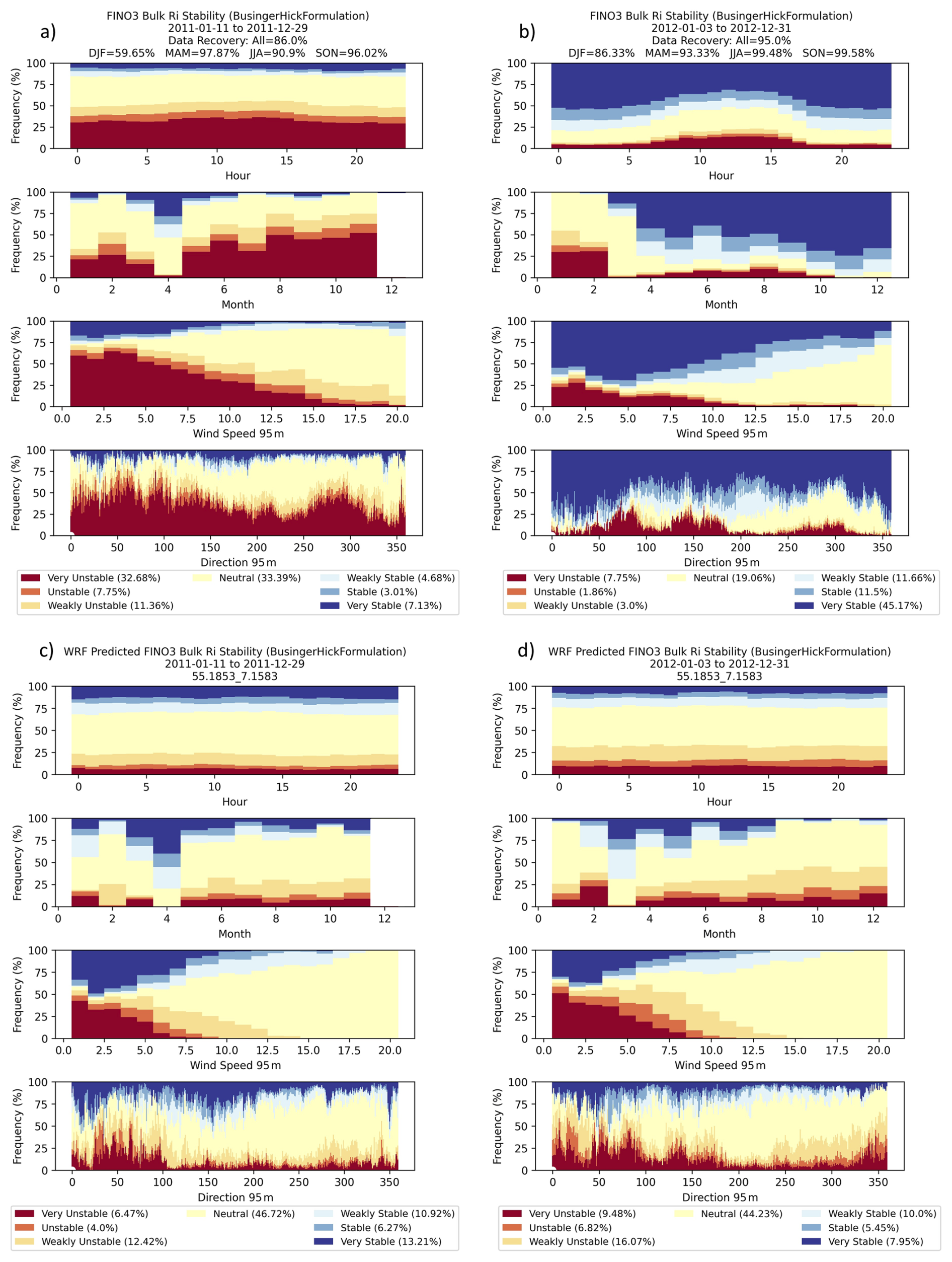
Figure 13Annual frequency (%) of Rib stability classes by the hour of day, month of year, wind speed, and wind direction for (a, b) FINO3 tower observations and (c, d) WRF concurrent time at FINO3 location. Results are shown for years 2011 (a, c) and 2012 (b, d). Note that December 2011 data are not available.
For this reason, it is also important to consider the difference in stability from a statistical distribution perspective, as shown in Fig. 14. The histograms of the Rib value, calculated every 10 min between 29 and 95 m a.m.s.l., confirm that 2012 and 2013 feature more frequent stable conditions when compared to 2010 and 2011. The stability shift is a direct result of increased values in the observed θv gradient between 2010 and 2011 to 2012 and 2013, whereas the vertical wind speed gradient stays consistent year to year (Figs. 14 and 15).

Figure 14Histograms of Rib (a, d, g, f), θv gradient (K m−1; b, e, h, k), and wind speed gradient (m s−1 m−1; c, f, i, l) between 29 and 95 m. Observations (gray) are compared to the WRF prediction (blue) at FINO3 for (a–c) 2010, (d–f) 2011, (g–i) 2012, and (j–l) 2013.
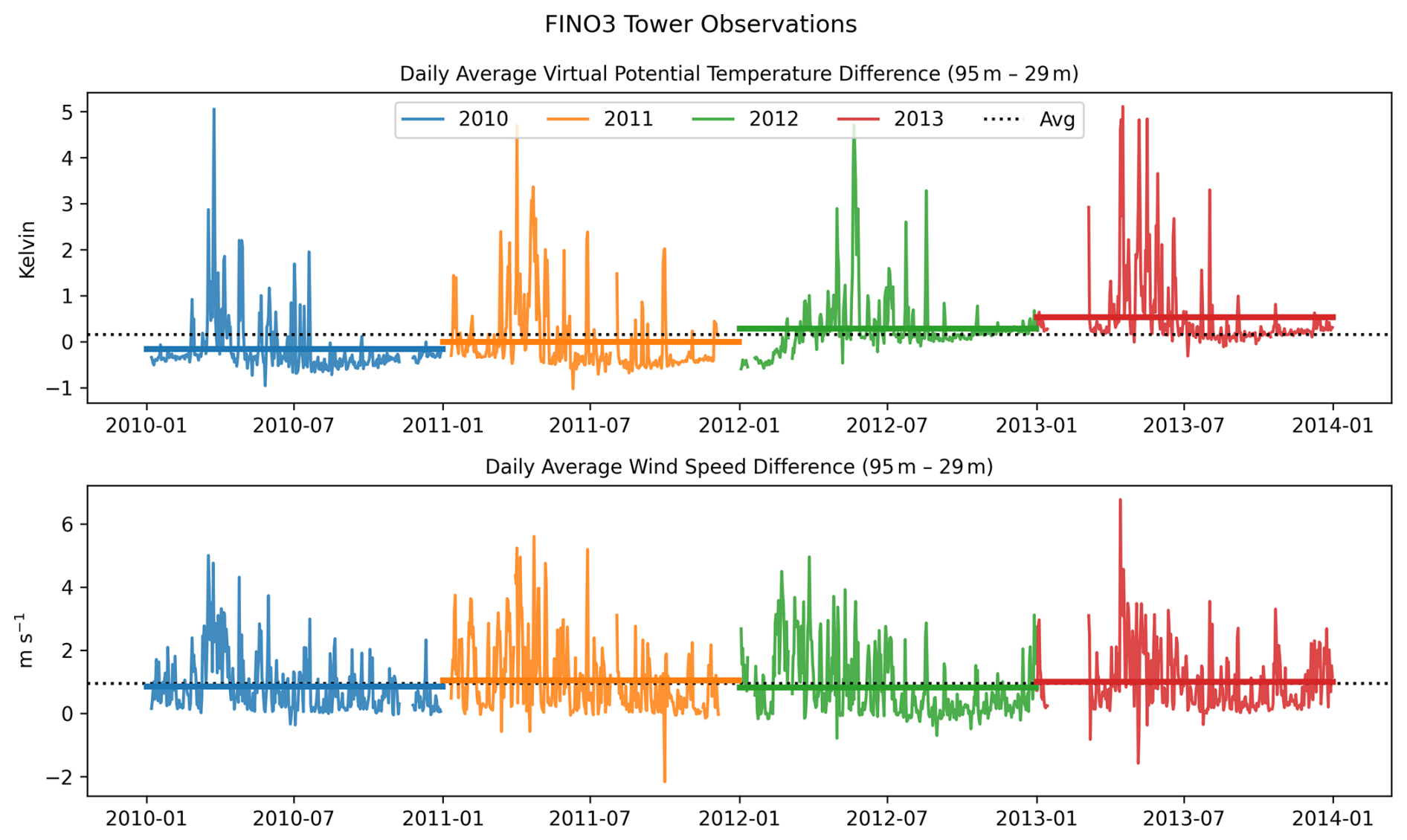
Figure 15Daily average difference in the θv (K; top) and the wind speed difference (m s−1; bottom) between 95 and 29 m a.m.s.l. for 2010 (blue), 2011 (orange), 2012 (green) and 2013 (red). Solid colored lines indicate the annual average difference, dashed black line is the average difference across the 4-year period.
However, regardless of stability classification, the same patterns of stability (seasonal, diurnal, wind regime) can be observed (Fig. 13). Unstable conditions are more common at lower wind speeds because of limited mixing (Fig. 13). Unstable conditions are also more frequent when winds are out of the east or southeast, which corresponds to a continental (Eurasian) air mass moving offshore (cold air moving over relatively warmer water). Overall, however, these results confirm that in the North Sea near-neutral to stable conditions are most common, especially when considering winds speeds relevant to wind energy (above a cut in speed ∼3 to 4 m s−1).
6.1 Model validation summary
The WIPAFF campaigns in 2016 and 2017 provided some of the first measurements of offshore wind farm waking, observed primarily during neutral and stable atmospheric conditions (Platis et al., 2018; Table 4). In this study, observations from the 41 WIPAFF flights and stationary measurements at the FINO3 tower are used to validate WRF's ability to predict long-range wakes behind large offshore wind farms. The results show that the model captures the wind speed deficit and wake length (commonly >50 km) well. However, there is a phase error in the WRF model of +/− 3 h that is corrected for by shifting the WRF time stamp to best match with observations. While time offsets are all found to occur within 3 h, from the cases analyzed, there is no pattern as to whether the time offset from WRF is before or after observations. This discrepancy is often due to prevailing wind conditions, as wind shifts can result in a lag between the model and observations, and cause more variation in the wake length and direction. Correcting for this time shift allows us to better examine the accuracy in the WRF model when capturing wind farm wakes and proves it is a reliable method for understanding the length, frequency, and stability characteristics that result in these long-range wakes. Other variables along the flight path such as wind direction, temperature (slight cold bias), specific humidity, and pressure show that overall WRF performance is good, but small wind direction errors are important to note as they can affect, for example, power production forecasting within and downwind of wind farms.
Model validation using the WIPAFF flight observations shows that under stable conditions the WRF model with the Fitch WFP parameterization well represents the wake behavior and atmospheric stability. However, given the limited sampling of predominately stable and neutral cases, from this analysis it is not possible to confirm a robust relationship between wake length and stability regime (Fig. 16).
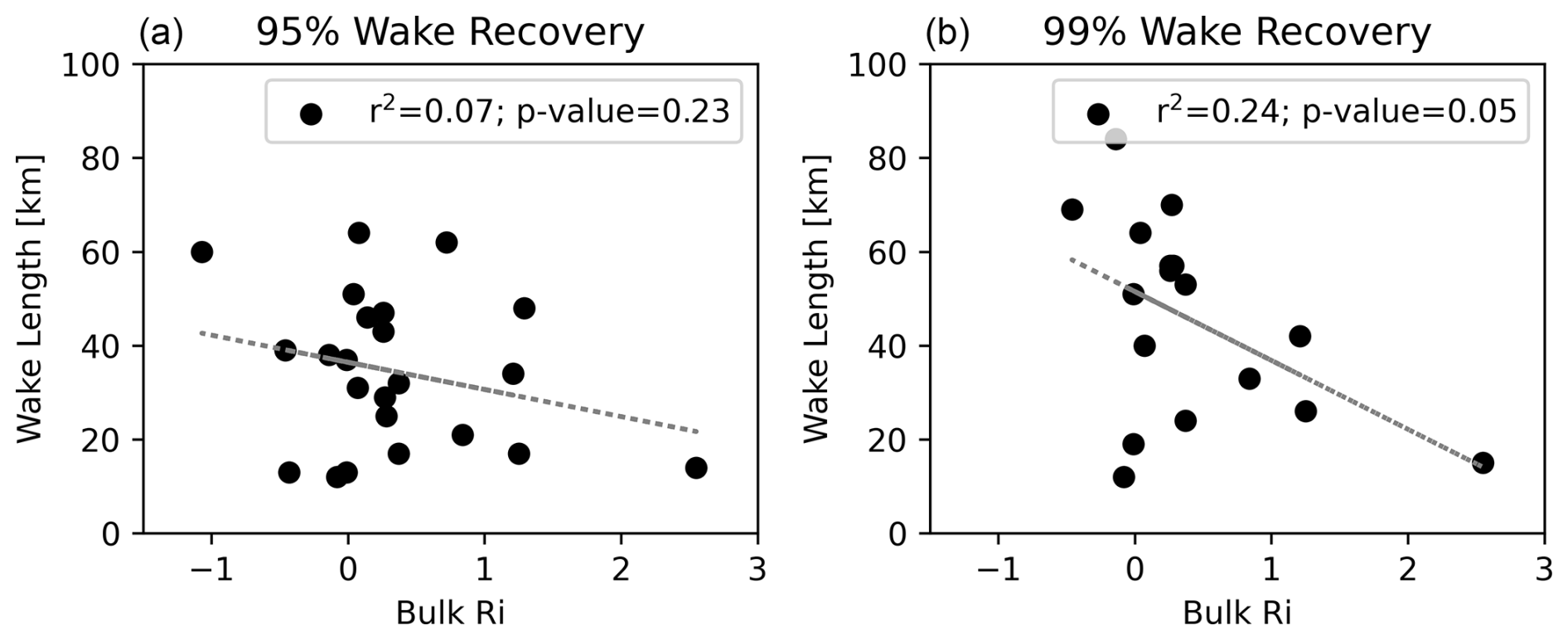
Figure 16Regression (using r2, the coefficient of determination) analysis of WRF results comparing (a) 95 % wake recovery length (km) and (b) 99 % wake recovery length to Rib for 25 WIPAFF flights that measure the downwind wake at hub height.
This is consistent with the results in Cimini et al. (2025), which note that prevailing offshore neutral conditions are a limitation when trying to understand model performance under offshore stability extremes (i.e., very unstable or very stable). While no linear relationship is found between the value of the Rib and the wake length for these selected cases, under stable conditions wakes are found to be upward of 50 km in length (Figs. 7 and 16), agreeing with claims in previous studies (Fitch et al., 2022; Ali et al., 2023; Platis et al., 2018; Cañadillas et al., 2020; Golbazi et al., 2022; Hahmann et al., 2025). For both the Rib and δ, the relationship is stronger between FINO3 and the WRF forecast then from flight measurements (Fig. 9). This not surprising, as the FINO3 tower is a stationary platform and will tend to have an overall better data sampling, as well as better spatial representativeness of the corresponding WRF output. One limitation of this dataset is the lack of extreme stability cases, so one cannot make conclusions on how wake activity will change during very stable or unstable conditions.
Based upon comparison with thermodynamic profiles available from the aircraft data, the Rib derived from WRF can be used as a reliable metric to classify stability using the Businger–Hicks formulation. Furthermore, the CIH derived from the WRF output and the flight profile observations compare well. Comparing the PBL height from WRF's standard output to the CIH derived from WRF's thermodynamic profiles show that, if necessary, the PBL height can be used as a rough estimate (Fig. 10c) of CIH in offshore environments.

Figure 17Regression (using r2, the coefficient of determination) analysis of WRF results comparing wake length (km) to (a) wind farm upwind wind speed (m s−1), (b) Rib value, and (c) PBL height (m). Points (open circles) are color coded by stability class.
6.2 Stability regimes in the North Sea
Using the results from Part 1, demonstrating reliability in using the WRF model to evaluate the long range wakes, further analysis is done to understand the met–ocean climatological characteristics of the North Sea in the context of offshore wind energy year-round. Focusing on how often the region can expect long-range wakes, the in situ measurements at the FINO3 tower are compared to the WRF model over a 4-year period (2010–2013; prior to when the FINO3 mast was surrounded by operational wind farms). Results show that the North Sea region experiences significant annual variation in wind direction and stability (Figs. 12 and 13). However, overall, the North Sea met–ocean environment is characterized by mostly neutral and near-neutral conditions.
Given the limitations of the data available from the WIPAFF flight campaign, this study focused on primarily on a subset stable and neutral cases. To confirm our hypothesis that stable stratification results in longer downwind wakes, a full-year WRF simulation run over the North Sea region allows for a comparison of wake length to a wider range of stability classes, including more very stable and very unstable cases. A subset of 22 cases is selected from the yearlong simulation run for 2012. These 22 d feature examples of unstable (7), neutral (8), and stable (7) conditions. Selecting examples during different stability regimes allows for analysis of the relationship between wind speed, Rib, and PBL height to the length of the external wind farm wake. As demonstrated, there is no relationship between wind speed and wake length (Fig. 17). However, these results confirm the hypothesis that more stable cases will result in longer wakes (Fig. 17; Fitch et al., 2022; Ali et al., 2023; Platis et al., 2018; Cañadillas et al., 2020; Golbazi et al., 2022; Hahmann et al., 2025). Also, a lower PBL height is often indicative of more stable conditions, and therefore, longer wakes (Fig. 17). Confirming this, wake length offshore is controlled by the stability regime rather than the wind speed. However, although there is no relationship between the wind speed and the wake length, wakes extending >50 km are generally below wind speeds of 13 m s−1, as higher wind speeds tend to be dominated by neutral well-mixed conditions (Fig. 17a).
The work in this study focuses on the ability of the WRF model using the Fitch WFP to predict long-range offshore wind farm wakes. While previous work has been done analyzing the potential for long-range wakes offshore (Golbazi et al., 2022; Rosencrans et al., 2024), a major limitation of those studies is the lack of validation from real data. Here, we focus on the North Sea, where research aircraft data are used to validate the ability of the Fitch WFP in the WRF modeling system to predict long-range wakes behind large offshore wind farms. The results show that the model is able to capture the wind speed deficit in the wake well and confirms previous findings that wakes exceed 50 km during stable conditions (Fitch et al., 2022; Ali et al., 2023; Platis et al., 2018; Cañadillas et al., 2020; Golbazi et al., 2022; Hahmann et al., 2025). Potentially significant errors, however, may arise from wind direction, as small errors can change the alignment of a wake with downwind wind farms and result in enhanced inter-farm waking. However, when comparing the flight observations to the WRF output, a time synching problem is noted; findings show the WRF model to be commonly offset from flight observations by up to 3 h.
As thermal stability is critical to understanding wake length, using thermodynamic profiles taken during research aircraft flights in addition to a 4-year meteorological analysis at the stationary FINO3 tower, different stability metrics are evaluated. Results show that the bulk Richardson number derived from the WRF model and observations compare well. A short-term (4-year) meteorological analysis of the wind environment and stability in the North Sea finds a persistence of mostly neutral to near-neutral conditions, with some inter-annual variability in both wind speed and stability regime. Leveraging the temporal and spatial coverage of modeling analysis with real observational data proves that under more stable conditions, downwind wakes extend further.
This is the first study to validate WRF model-derived Rib and CIH using observed thermodynamic profiles in offshore regions. The findings in this study can be applied to other regions with existing wind farms or undergoing offshore wind energy development and can facilitate establishing a robust climatological analysis of wind regimes and stability, providing a better understanding of conditions favorable for long-range wind farm wakes.
Information on the FINO towers can be found and downloaded at https://www.bsh.de/DE/DATEN/daten_node.html (last access: 31 October 2026).
The WIPAFF flight data can be found and downloaded at https://doi.org/10.1594/PANGAEA.902845 (Bärfuss et al., 2019).
JF, PB, and EM conceptualized the project and obtained funding and resources for the work. PB and NR provided the data, EM processed the data used for model evaluation and preformed the WRF simulations with the assistance of PB and AG. EM conducted the analysis, produced the figures, and interpreted results with supervision and input from PB, JF, and NR. EM prepared the initial draft and all authors reviewed and edited the publication.
The contact author has declared that none of the authors has any competing interests.
The views expressed in the article do not necessarily represent the views of the NSF or the US government.
Publisher's note: Copernicus Publications remains neutral with regard to jurisdictional claims made in the text, published maps, institutional affiliations, or any other geographical representation in this paper. The authors bear the ultimate responsibility for providing appropriate place names. Views expressed in the text are those of the authors and do not necessarily reflect the views of the publisher.
This work utilized the computing resources at UL Solutions and the Atmospheric Sciences Research Center (ASRC) at the University at Albany. Data storage was supported by UL Solutions and ASRC. Funding was provided by National Science Foundation (NSF) through a funded internship program.
This research was funded by the National Science Foundation Internship Program Fellowship (grant no. 1183904-2-98042).
This paper was edited by Astrid Lampert and reviewed by four anonymous referees.
Ali, K., Schultz, D. M., Revell, A. Stallard, T., and Ouro, P.: Assessment of Five Wind-Farm Parameterizations in the Weather Research and Forecasting Model: A Case Study of Wind Farms in the North Sea, Mon. Weather Rev., 151, 2333–2359, https://doi.org/10.1175/MWR-D-23-0006.1, 2023.
Archer, C. L., Colle, B. A., Veron, D. L., Veron, F., and Sienkiewicz, M. J.: On the predominance of unstable atmospheric conditions in the marine boundary layer offshore of the U.S. northeastern coast, J. Geophys. Res.-Atmos., 121, 8869–8885, https://doi.org/10.1002/2016JD024896, 2016.
Archer, C. L., Wu, S., Ma, Y., and Jiménez, P.: Two corrections for turbulent kinetic energy generated by wind farms in the WRF Model, Mon. Weather Rev., 148, 4823–4835, https://doi.org/10.1175/MWR-D-20-0097.1, 2020.
Ball, F. K.: Control of inversion height by surface heating, Q. J. Roy. Meteor. Soc., 86, 483–494, https://doi.org/10.1002/qj.49708637005, 1960.
Bärfuss, K., Hankers, R., Bitter, M., Feuerle, T., Schulz, H., Rausch, T., Platis, A., Bange, J., and Lampert, A.: In-situ airborne measurements of atmospheric and sea surface parameters related to offshore wind parks in the German Bight, PANGAEA [data set], https://doi.org/10.1594/PANGAEA.902845, 2019.
Barthelmie, R. J.: The effects of atmospheric stability on coastal wind climates, Meteorol. Appl., 6, 39–47, https://doi.org/10.1017/S1350482799000961, 1999.
Berge, K., Centurelli, G., Dörenkämper, M., Bange, J., and Platis, A.: Evaluation of Engineering Models for Large-Scale Cluster Wakes With the Help of In Situ Airborne Measurements, Wind Energy, 27, 1040–1062, https://doi.org/10.1002/we.2942, 2024.
Brower, M. and Robinson, N.: The openwind deep-array wake model: development and validation, Technical Report, AWS Truepower, Albany, NY, 15 pp., https://www.ul.com/sites/default/files/2024-11/UL_Solutions_Deep-Array-Wake-Model_Validation_2024.pdf (last access: 31 October 2026), 2009.
Cañadillas, B., Foreman, R., Barth, V., Siedersleben, S., Lampert, A., Platis, A., Djath, B., Schulz-Stellenfleth, J., Bange, J., Emeis, S., and Neumann, T.: Offshore wind farm wake recovery: Airborne measurements and its representation in engineering models, Wind Energy, 23, 1165–1366, https://doi.org/10.1002/we.2484, 2020.
Cañadillas, B., Beckenbauer, M., Trujillo, J. J., Dörenkämper, M., Foreman, R., Neumann, T., and Lampert, A.: Offshore wind farm cluster wakes as observed by long-range-scanning wind lidar measurements and mesoscale modeling, Wind Energ. Sci., 7, 1241–1262, https://doi.org/10.5194/wes-7-1241-2022, 2022.
Cantero, E., Sanz, J., Borbon, F., Paredes, D., and Garcia, A.: On the measurement of stability parameters over complex mountainous terrain, Wind Energy Science, 7, 221–235, 2022.
Christiansen, M. B. and Hasager, C. B.: Wake effects of large offshore wind farms identified from satellite SAR, Remote Sens. Environ., 98, 251–268, https://doi.org/10.1016/j.rse.2005.07.009, 2005.
Christiansen, M. B. and Hasager, C. B.: Using airborne and satellite SAR for wake mapping offshore, Wind Energy, 9, 437–455, https://doi.org/10.1002/we.196, 2006.
Cimini, D., Gandoin, R., Fiedler, S., Acquistapace, C., Balotti, A., Gentile, S., Geraldi, E., Knist, C., Martinet, P., Nilo, S. T., Pace, G., Pospichal, B., and Romano, F.: Atmospheric stability from numerical weather prediction models and microwave radiometer observations for onshore and offshore wind energy applications, Atmos. Meas. Tech., 18, 2041–2067, https://doi.org/10.5194/amt-18-2041-2025, 2025.
Corsmeier, U., Hankers, R., and Wieser, A.: Airborne turbulence measurements in the lower troposphere onboard the research aircraft Dornier 128-6, D-IBUF, Meteorol. Z., 10, 315–329, https://doi.org/10.1127/0941-2948/2001/0010-0315, 2001.
Deardorff, J. W.: Prediction of convective mixed-layer entrainment for realistic capping inversion structure, J. Atmos. Sci., 36, 424–436, https://doi.org/10.1175/1520-0469(1979)036<0424:POCMLE>2.0.CO;2, 1979.
Debnath, M., Scholbrock, A. K., Zalkind, D., Moriarty, P., Simley, E., Hamilton, N., Ivanov, C., Arthur, R. S., Barthelmie, R., Bodini, N., Brewer, A., Goldberger, L., Herges, T., Hirth, B., Iungo, G. V., Jager, D., Kaul, C., Klein, R., Krishnamurthy, R., Letizia, S., Lundquist, J. K., Maniaci, D., Newsom, R., Pekour, M., Pryor, S. C., Ritsche, M. T., Roadman, J., Schroeder, J., Shaw, W. J., Van Dam, J., and Wharton, S.: Design of the American Wake Experiment (AWAKEN) field campaign, J. Phys., 2265, https://doi.org/10.1088/1742-6596/2265/2/022058, 2022.
Djath, B., Schulz-Stellenfleth, J., and Cañadillas, B.: Impact of atmospheric stability on X-band and C-band Synthetic Aperture Radar imagery of offshore windpark wakes, J. Renew. Sustain. Ener., 10, https://doi.org/10.1063/1.5020437, 2018.
Djath, B., Schulz-Stellenfleth, J., and Cañadillas, B.: Study of Coastal Effects Relevant for Offshore Wind Energy Using Spaceborne Synthetic Aperture Radar (SAR), Remote Sens., 14, 1688, https://doi.org/10.3390/rs14071688, 2022.
Emeis, S.: A simple analytical wind park model considering atmospheric stability, Wind Energy, 13, 459–469, https://doi.org/10.1002/we.367, 2010.
European Centre for Medium-Range Weather Forecasts (ECMWF): Global reanalysis: goodbye ERA-Interim, hello ERA5, https://www.ecmwf.int/en/newsletter/159/meteorology/global-reanalysis-goodbye-era-interim-hello-era5 (last access: 21 March 2023), 2019.
Fischereit, J., Brown, R., Larsén, X. G., Badger, J., and Hawkes, G.: Review of Mesoscale Wind-Farm Parametrizations and their Applications, Bound.-Lay. Meteorol., 182, 175–224, https://doi.org/10.1007/s10546-021-00652-y, 2021.
Fischereit, J., Schaldemose Hansen, K., Larsén, X. G., van der Laan, M. P., Réthoré, P.-E., and Murcia Leon, J. P.: Comparing and validating intra-farm and farm-to-farm wakes across different mesoscale and high-resolution wake models, Wind Energ. Sci., 7, 1069–1091, https://doi.org/10.5194/wes-7-1069-2022, 2022.
Fitch, A. C., Olson, J. B., Lundquist, J. K., Dudhia, J., Gupta, A. K., Michalakes, J., and Barstad, I.: Local and Mesoscale Impacts of Wind Farms as Parameterized in a Mesoscale NWP Model, Mon. Weather Rev., 140, 3017–3038, https://doi.org/10.1175/MWR-D-11-00352.1, 2022.
Floors, R., Gryning, S., Peña, A., and Batchvarova, E.: Analysis of diabatic flow modification in the internal boundary layer, Meteorol. Z., 20, 649–659, https://doi.org/10.1127/0941-2948/2011/0290, 2011.
Foreman, R. J., Cañadillas, B., and Robinson, N.: The Atmospheric Stability Dependence of Far Wakes on the Power Output of Downstream Wind Farms, Energies, 17, 488, https://doi.org/10.3390/en17020488, 2024.
García-Díez, M., Fernández, J., Fita, L., and Yagüe, C.: Seasonal dependence of WRF model biases and sensitivity to PBL schemes over Europe, Q. J. Roy. Meteor. Soc., 139, 501–514, https://doi.org/10.1002/qj.1976, 2013.
Garstang, M. and Fitzjarrald, D. R.: Observations of Surface to Atmosphere Interactions in the Tropics, Oxford University Press, 405 pp., 1999.
Golbazi, M., Archer, C., and Alessandrini, S.: Surface impacts of large offshore wind farms, Environ. Res. Lett., 17, https://doi.org/10.1088/1748-9326/ac6e49, 2022.
Hahmann, A. N., Imberger, M., Fischereit, J., Alonso-de-Linaje, N. G., and Badger, J.: Environmental Mapping and Screening of the Offshore Wind Potential in Denmark: Sensitivity mapping: Wind, DTU Wind and Energy Systems, https://orbit.dtu.dk/en/publications/environmental-mapping-and-screening-of-the-offshore-wind-potentia/ (last access: 31 October 2026) 2025.
Hansen, K. S., Barthelmie, R. J., Jensen, L. E., and Sommer, A.: The impact of turbulence intensity and atmospheric stability on power deficits due to wind turbine wakes at Horns Rev wind farm, Wind Energy, 15, 183–196, https://doi.org/10.1002/we.512, 2012.
Hasager, C. B., Vincent, P., Badger, J., Badger, M., Di Bella, A., Peña, A., Husson, R., and Volker, P. J. H.: Using Satellite SAR to Characterize the Wind Flow around Offshore Wind Farms, Energies, 8, https://doi.org/10.3390/en8065413, 2015.
Hersbach, H., Bell, B., Berrisford, P., Hirahara, S., Horányi, A., Muñoz-Sabater, J., Nicolas, J., Peubey, C., Radu, R., Schepers, D., Simmons, A., Soci, C., Abdalla, S., Abellan, X., Balsamo, G., Bechtold, P., Biavati, G., Bidlot, J., Bonavita, M., De Chiara, G., Dahlgren, P., Dee, D., Diamantakis, M., Dragani, R., Flemming, J., Forbes, R., Fuentes, M., Geer, A., Haimberger, L., Healy, S., Hogan, R. J., Hólm, E., Janisková, M., Keeley, S., Laloyaux, P., Lopez, P., Lupu, C., Radnoti, G., de Rosnay, P., Rozum, I., Vamborg, F., Villaume, S., and Thépaut, J.: The ERA5 global reanalysis, Q. J. Roy. Meteor. Soc., 146, 1999–2049, https://doi.org/10.1002/qj.3803, 2020.
Kihlström, L.: How Horns Rev 1 paved the way for offshore wind, Vattenfall, https://group.vattenfall.com/press-and-media/newsroom/2023/how-horns-rev-1-paved-the-way-for-offshore-wind (last access: 5 May 2025), 2023.
Krishnamurthy, R., Newsom, R. K., Kaul, C. M., Letizia, S., Pekour, M., Hamilton, N., Chand, D., Flynn, D., Bodini, N., and Moriarty, P.: Observations of wind farm wake recovery at an operating wind farm, Wind Energ. Sci., 10, 361–380, https://doi.org/10.5194/wes-10-361-2025, 2025.
Lundquist, J. K., DuVivier, K. K., Kaffine, D., and Tomaszewski, J. M.: Costs and consequences of wind turbine wake effects arising from uncoordinated wind energy development, Nature Energy, 4, 26–34, https://doi.org/10.1038/s41560-019-0363-9, 2019.
Ma, Y., Archer, C. L., and Vasel-Be-Hagh, A.: Comparison of individual versus ensemble wind farm parameterizations inclusive of sub-grid wakes for the WRF model, Wind Energy, 25, https://doi.org/10.1002/we.2758, 2022.
McCabe, E. J. and Freedman, J. M.: Quantifying the uncertainty in the weather research and forecasting model under sea breeze and low-level jet conditions in the New York Bight: Importance to offshore wind energy, Weather Forecast., 40, https://doi.org/10.1175/WAF-D-22-0119.1, 2025.
Mohan, M. and Siddiqui, T. A.: Analysis of various schemes for the estimation of atmospheric stability classification, Atmos. Environ., 32, 3775–3781, 1998.
Monin, A. S. and Obukhov, A. M.: Basic laws of turbulent mixing in the surface layer of the atmosphere, Tr. Akad. Nauk SSSR Geophiz. Inst, 24, 163–187, 1954.
Nakanishi, M. and Niino, H.: An Improved Mellor-Yamada Level 3 Model: Its Numerical Stability and Application to a Regional Prediction of Advection Fog, Bound.-Lay. Meteorol., 119, 397–407, https://doi.org/10.1007/s10546-005-9030-8, 2006.
Nakanishi, M. and Niino, H.: Development of an improved turbulence closure model for the atmospheric boundary layer, J. Meteor. Soc. Japan, 87, 895–912, https://doi.org/10.2151/jmsj.87.895, 2009.
National Renewable Energy Laboratory (NREL): The American WAKE experimeNt (AWAKEN): Groundbreaking International Field Research Addresses Wind Farm Atmospheric Interactions, https://www.energy.gov/sites/default/files/2022-01/AWAKEN-fact-sheet.pdf (last access: 31 October 2026), 2022.
Nygaard, N. G., Steen, S. T., Poulsen, L., and Pedersen, J. G.: Modelling cluster wakes and wind farm blockage, J. Phys. Conf. Ser., 1618, 062072, https://doi.org/10.1088/1742-6596/1618/6/062072, 2020.
Olsen, B. T., Hahmann, A. N., Sempreviva, A. M., Badger, J., and Jørgensen, H. E.: An intercomparison of mesoscale models at simple sites for wind energy applications, Wind Energ. Sci., 2, 211–228, https://doi.org/10.5194/wes-2-211-2017, 2017.
Olson, J. B., Kenyon, J. S., Angevine, W. A., Brown, J. M., Pagowski, M., and Sušelj, K.: A description of the MYNN EDMF scheme and the coupling to other components in WRF–ARW, NOAA Tech. Memo, OAR GSD 61, 42 pp., https://doi.org/10.25923/n9wm-be49, 2019.
Ørsted: Making green energy affordable, 28 pp., https://orsted.com/-/media/WWW/Docs/Corp/COM/explore/Making-green-energy-affordable-June-2019.pdf (last access: 31 October 2026), 2019.
Pedersen, J. G., Svensson, E., Poulsen, L., and Nygaard, N. G.: Turbulence Optimized Park model with Gaussian wake profile, J. Phys. Conf. Ser., 2265, https://doi.org/10.1088/1742-6596/2265/2/022063, 2022.
Platis, A., Siedersleben, S. K., Bange, J., Lampert, A., Bärfuss, K., Hankers, R., Cañadillas, B., Foreman, R., Schulz-Stellenfleth, J., Djath, B., Neumann, T., and Emeis, S.: First in situ evidence of wakes in the far field behind offshore wind farms, Sci. Rep., 8, https://doi.org/10.1038/s41598-018-20389-y, 2018.
Platis, A., Bange, J., Bärfuss, K., Cañadillas, B., Hundhausen, M., Djath, B., Lampert, A., Schulz-Stellenfleth, J., Siedersleben, S., Neumann, T., and Emeis, S.: Long-range modifications of the wind field by offshore wind parks – results of the project WIPAFF, Meteorol. Z., 29, 355–367, https://doi.org/10.1127/metz/2020/1023, 2020.
Porchetta, S., Munters, W., Lejeune, M., Borgers, R., Buckingham, S., and Howland, M. F.: Annual wake impacts in and between wind farm clusters – Part 1: WRF-simulated wake losses for different atmospheric conditions, Wind Energ. Sci., 11, 3273–3294, https://doi.org/10.5194/wes-11-3273-2026, 2026.
Pronk, V., Bodini, N., Optis, M., Lundquist, J. K., Moriarty, P., Draxl, C., Purkayastha, A., and Young, E.: Can reanalysis products outperform mesoscale numerical weather prediction models in modeling the wind resource in simple terrain?, Wind Energ. Sci., 7, 487–504, https://doi.org/10.5194/wes-7-487-2022, 2022.
Pryor, S. C. and Barthelmie, R. J.: Power Production, Inter- and Intra-Array Wake Losses from the U.S. East Coast Offshore Wind Energy Lease Areas, Energies, 17, https://doi.org/10.3390/en17051063, 2024.
Rampanelli, G. and Zardi, D.: A Method to Determine the Capping Inversion of the Convective Boundary Layer, J. Appl. Meteorol. Clim., 43, 925–933, https://doi.org/10.1175/1520-0450(2004)043<0925:AMTDTC>2.0.CO;2, 2004.
Rausch, T., Bärfuss, K., Hankers, R., Bitter, M., Feuerle, T., Cremer, M., Angermann, M., Füllgraf, J., and Lampert, A.: In-situ airborne measurements of atmospheric and sea surface parameters related to offshore wind parks in the German Bight, PANGAEA [data set], https://doi.org/10.1594/PANGAEA.955382, 2023.
Rogers, J. D.: Experimental evaluation of wind turbine wake turbulence impacts on a general aviation aircraft, Wind Energ. Sci., 9, 1849–1868, https://doi.org/10.5194/wes-9-1849-2024, 2024.
Rosencrans, D., Lundquist, J. K., Optis, M., Rybchuk, A., Bodini, N., and Rossol, M.: Seasonal variability of wake impacts on US mid-Atlantic offshore wind plant power production, Wind Energ. Sci., 9, 555–583, https://doi.org/10.5194/wes-9-555-2024, 2024.
Ruisi, R. and Bossanyi, E.: Engineering models for turbine wake velocity deficit and wake deflection. A new proposed approach for onshore and offshore applications, J. Phys. Conf. Ser., 1222, https://doi.org/10.1088/1742-6596/1222/1/012004, 2019.
Siedersleben, S. K., Lundquist, J. K., Platis, A., Bange, J., Bärfuss, K., Lampert, A., Cañadillas, B., Neumann, T., and Emeis, S.: Micrometeorological impacts of offshore wind farms as seen in observations and simulations, Environ. Res. Lett., 13, https://doi.org/10.1088/1748-9326/aaea0b, 2018.
Skamarock, W. C., Klemp, B., Dudhia, J., Gill, O., Liu, Z., Berner, J., Wang, W., Powers, G., Duda, G., Barker, D., and Huang, X.: A Description of the Advanced Research WRF Model Version 4.3, NCAR/TN-556+STR, Mesoscale and Microscale Meteorology Division, National Center for Atmospheric Research, Boulder, https://doi.org/10.5065/1dfh-6p97, 2021.
Stoelinga, M., Sanchez-Gomez, M., Poulos, G., and Crescenti, J.: Estimating Long-Range External Wake Losses in Energy Yield and Operational Performance Assessments Using the WRF Wind Farm Parameterization, Technical report, ArcVera, 19 pp., https://arcvera.com/wp-content/uploads/2022/08/ArcVera-White-Paper-Estimating-Long-Range-External (last access: 4 January 2025), 2022.
Stull, R. B.: An Introduction to Boundary Layer Meteorology, Kluwer Academic Publishers, ISBN 978-9027727695, 1988.
Tennekes, H.: A Model for the Dynamics of the Inversion Above a Convective Boundary Layer, J. Atmos. Sci., 30, 558–567, https://doi.org/10.1175/1520-0469(1973)030<0558:AMFTDO>2.0.CO;2, 1973.
Vattenfall: Horns Rev 1, https://powerplants.vattenfall.com/horns-rev/ (last access: 5 May 2025), 2025.
Wang, Z., Yuan, J., Wood, R., Chen, Y., and Tong, T.: Profile-based estimated inversion strength, Atmos. Chem. Phys., 23, 3247–3266, https://doi.org/10.5194/acp-23-3247-2023, 2023.
Wood, R. and Bretherton, C. S.: On the Relationship between Stratiform Low Cloud Cover and Lower-Tropospheric Stability, J. Climate, 19, 6425–6432, https://doi.org/10.1175/JCLI3988.1, 2006.
Xia, G., Cervarich, M. C., Roy, S. B., Zhou, L., Minder, J. R., Jimenez, P. A., and Freedman, J. M.: Simulating Impacts of Real-World Wind Farms on Land Surface Temperature Using the WRF Model: Validation with Observations, Mon. Weather Rev., 145, 4813–4836, https://doi.org/10.1175/MWR-D-16-0401.1, 2017.
Zhan, L., Letizia, S., and Iungo, G. V.: Optimal tuning of engineering wake models through lidar measurements, Wind Energ. Sci., 5, 1601–1622, https://doi.org/10.5194/wes-5-1601-2020, 2020.