
the Creative Commons Attribution 4.0 License.
the Creative Commons Attribution 4.0 License.
 | 17 Nov 2026
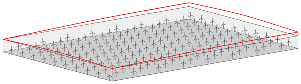
Fast models for blockage and gravity-wave effects on wind-farm power output

Johan Meyers
Large offshore wind farms can trigger atmospheric gravity waves, with the associated hydrostatic blockage effect impacting their energy yield. Unfortunately, to date no tools exist that can model this wind-farm–gravity-wave interaction and blockage at a computational cost that is not drastically higher than conventional engineering wake models. To address this, this paper develops ways of speeding up atmospheric perturbation models (APMs) by an order of magnitude by applying insights from the recently proposed two-scale momentum (2SM) theory (Nishino and Dunstan, 2020, A2). This leads to two different models, with one using pre-computed farm-level coefficients to compute the turbine forces and power output, while the other relies on repeated wake model evaluations. The core 2SM hypothesis of scale separation and both developed models are validated using a prior LES dataset of a large rectangular wind farm with regular spacing and constant thrust coefficients. In this idealized setup, both fast 2SM–APMs perform well, predicting blockage-corrected farm power at a computational cost that is only a factor 35 slower than a standalone wake model.
- Article
(2509 KB) - Full-text XML
- BibTeX
- EndNote


As offshore wind turbines and farms continue to grow in both size and installed capacity, they reach the point where they form an obstacle to the entire atmospheric boundary layer (ABL) (Bleeg et al., 2018). Large eddy simulation (LES) studies have shown that in conventionally neutral boundary layers (CNBLs), where a neutral ABL is topped by a capping inversion and a stratified upper atmosphere, wind farms can trigger gravity waves, creating upstream pressure gradients and blockage effects (Allaerts and Meyers, 2017, 2018; Centurelli et al., 2021; Lanzilao and Meyers, 2022, 2023a, 2024; Maas, 2023a, b; Stipa et al., 2024b). As these mesoscale effects affect turbine power output, they are becoming more important to farm operation and planning.
Currently, conventional engineering tools rely on the superposition of individual turbine effects, thereby implicitly assuming that their aggregate effect is not larger than the sum of its parts (Porté-Agel et al., 2020). These wake models (WMs) remain widely used because of their low computational cost, which makes them well-suited for farm planning, control, and annual energy production estimates. In contrast, computational fluid dynamics (CFD) methods like Reynolds-averaged Navier–Stokes (RANS), LES, or mesoscale climate models are able to capture most of the relevant flow phenomena. However, their high cost prevents them from being widely used for fast farm power predictions (Meyers et al., 2022).
Installing and operating the next generation of offshore wind farms will therefore require new models that can simulate the generation of blockage and gravity waves, while keeping the computational cost orders of magnitude below conventional CFD methods. One promising recently developed tool that fits these requirements is the atmospheric perturbation model (APM) (Allaerts and Meyers, 2019; Devesse et al., 2024a; Stipa et al., 2024a). Building on earlier work by Smith (2010), this model simulates large-scale wind-farm–atmosphere interactions explicitly, while coupling to conventional wake models to account for turbine-scale flow effects. In order to capture the local feedback effects between the turbine forces and the mesoscale flow, the governing system of equations is solved repeatedly in a fixed-point iteration. This constitutes the main cost of the model, which is low compared to conventional CFD tools but still several hundred to a thousand times higher than standard wake models (Devesse et al., 2024b).
One way to further simplify and speed up the modeling of wind-farm–atmosphere interactions is the two-scale momentum (2SM) framework introduced by Nishino and Dunstan (2020). At its core, this approach assumes a separation between the turbine- and farm-scale flows. As a result of this hypothesis, variations in farm power output due to mesoscale effects are fully determined by the associated changes in the average velocity over the farm. Based on high-fidelity LES results, this hypothesis has been confirmed for large wind farms in idealized conditions (Kirby et al., 2022, 2025).
Other recent studies have proposed wind farm models relying on similar ideas of scale separation. van der Laan et al. (2023) and Stipa et al. (2024c) proposed actuator-farm models for RANS and LES, respectively, allowing these methods to simulate wind farms without resolving the turbine-scale flow. Similarly, Du et al. (2025) developed a wind-farm parametrization for mesoscale weather models, which due to their kilometer-scale resolution cannot represent individual turbines, based on matching the average velocity in the farm between the mesoscale model and a wake model. However, since these studies are not as explicit in their theoretical treatment of this scale separation, we will refer to the overall idea as the two-scale momentum approach, following Nishino and Dunstan (2020).
Our goal is to develop fast models for predicting wind-farm power output that account for blockage and gravity-wave effects. To that end, the 2SM framework can be useful, as it implies that flow solvers simulating the farm-scale flow do not have to resolve the turbine-scale flow. This would allow for coarser grid resolutions and reduced computational costs. However, even when using coarser grids, conventional CFD tools are still multiple orders of magnitude slower than engineering wake models (Ouro et al., 2025). In contrast, the APM already uses a coarse resolution, while its main cost lies in capturing the local feedback effects between the turbine forces and the mesoscale flow. Therefore, we focus on combining the 2SM and APM approaches, leveraging insights from the former to speed up and simplify the latter.
Since, according to the 2SM hypothesis, a farm's power output only depends on the average velocity in the farm, the APM may neglect local changes in the turbine force distribution within the farm induced by gravity-wave effects. Instead, this force distribution can be scaled uniformly over the farm to match the total farm force as predicted by 2SM theory. Due to the linear nature of the APM, this transforms the model's governing equations into a system of scalar equations, drastically lowering its computational cost. We use this to develop two versions of the sped-up APM, one which uses farm thrust and power coefficients to model the farm, following earlier 2SM studies and one which is directly coupled to a standard wake model. Both models are validated using the LES dataset of a large wind farm operating in idealized CNBL conditions from Lanzilao and Meyers (2024).
The remainder of this paper is outlined as follows. Section 2 provides an overview of 2SM theory and demonstrates its core hypothesis using the LES results of Lanzilao and Meyers (2024). Section 3 then introduces the APM's governing equations and how they are solved. Combining these two, Sect. 4 shows how a 2SM–APM can cheaply calculate a farm's power output if its farm-level thrust and power coefficients are known. Building on this, Sect. 5 develops an alternative method that couples the farm-averaged APM output directly to a wake model, thereby eliminating the need for these farm coefficients but requiring repeated wake model evaluations. Section 6 compares the performance, advantages, and limitations of both models. Finally, Sect. 7 gives an overview of the results and an outlook for future research.
Recently, Kirby et al. (2025) demonstrated that the 2SM theory developed by Nishino and Dunstan (2020) can be used to simplify the interaction between mesoscale atmospheric flows and wind farm operation. The core hypothesis of 2SM theory is a separation of internal and external effects and the associated spatial scales. Internal effects, such as turbine setpoints and wakes, determine the ratios of the individual turbine disk velocities Sk to the average streamwise velocity Uf in the farm region. External effects, such as large-scale momentum advection, entrainment above the farm, or gravity-wave-induced pressure gradients, act on the farm scale and affect the average velocity within the farm Uf. The total farm power Pf can then be expressed as
where ρ is the air density, Af is the total rotor area of the farm turbines, is the internal farm power coefficient, Nt is the number of turbines, and Ak and are the turbine disk areas and disk-based power coefficients, respectively, with k indicating the turbine number.
Nishino and Dunstan (2020) make an analogous argument for the farm thrust, so that
where F is the total farm force (scaled with air density), is the farm thrust coefficient, and are the disk-based turbine thrust coefficients. Like , the internal farm thrust coefficient is assumed to only depend on the internal problem.
Kirby et al. (2025) investigated this assumption using LES results of large wind farms with uniform turbine densities in below-rated conditions, so that the are constant over the farm. They found that the internal power coefficient as defined in Eq. (1) is a good heuristic for internal effects, and remained constant over cases with different mesoscale flow behavior. This then implies that can be calculated using small-scale simulations of the same farm or engineering wake models, while the problem of including mesoscale stratification effects in farm power calculations is simplified to solving only the external problem, i.e., estimating Uf.
We demonstrate this by taking from a neutral flow simulation and Uf from different CNBL simulations with different meso-scale stratification effects but the same farm layout and geostrophic wind speed. We then estimate the power produced in the CNBL cases using Eq. (1) and compare it against the actual production. For this, we use the prior LES dataset from Lanzilao and Meyers (2024), which consists of 36 simulations of the same large wind farm in idealized steady CNBL conditions (Lanzilao and Meyers, 2023b), which was also used by Kirby et al. (2025). This farm has 160 10 MW turbines, arranged uniformly in a rectangular staggered layout, operating at below-rated conditions, with the disk-based thrust coefficients fixed to . Each simulation has a different combination of boundary layer heights H, capping inversion strengths Δθ, and atmospheric lapse rates Γ. The different cases are identified with these parameters, so that H500-Δθ5-Γ4 denotes the case with the precursor profile initialized with these values. For each boundary layer height, the dataset also includes simulations of a wind-farm in truly neutral flow and of a stand-alone turbine with Δθ=5 K and Γ=4 K km−1. A detailed description of the LES setup and results is given by Lanzilao and Meyers (2024).
We calculate Uf as a straightforward average over the wind farm, so that
where Hf is the height of the 2SM averaging volume, and Ωf the planform area of the wind farm. We take Ωf to be a rectangle around the farm edge, thereby including the outer edges of the turbine disks at the sides. We set the height Hf of the volume to twice the turbine hub height zh, as this corresponds to the setup of the APM (see Sect. 4.1). This height is above the turbine tip height but below the ABL height for all the cases in the dataset of Lanzilao and Meyers (2024). While some of the H150 cases have lower unperturbed ABL heights, strong vertical displacements of the capping inversions over the wind farm ensure that even there the ABL height is above the 2SM control volume. The exact dimensions of the resulting control volume are listed in Table 1. This simple approach is possible because the analyzed farm has a convex and uniform layout. More realistic farms might require a more complex horizontal averaging method such as the one proposed by van der Laan et al. (2023), where the wind speed is weighted by Gaussian distributions centered around the turbines. Alternatively, a farm could be split in two or more homogeneous regions. Further investigation of such approaches is beyond the scope of this study and left as promising future work.
Table 1Specification of the 2SM farm averaging volume for the cases of Lanzilao and Meyers (2024).
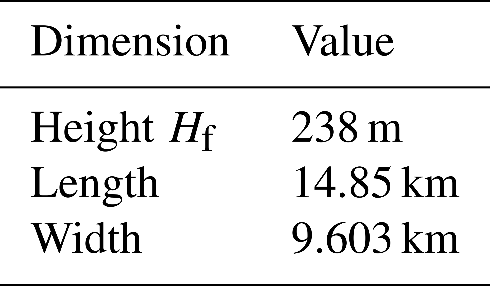
To calculate , we use the 3D time-averaged velocity fields of case H500-Δθ0-Γ0. After averaging the streamwise velocity field to obtain Uf, we obtain from Eq. (1). Subsequently, the farm power outputs for the 36 CNBL cases are calculated by averaging their Uf and combining it with the prior through Eq. (1). In order to avoid issues with the power calculation in LES related to the used actuator-disk method and grid size (Shapiro et al., 2019), the resulting power outputs are scaled with the power outputs P0 of standalone turbines operating at the same inflow wind speeds, as was done by Lanzilao and Meyers (2024). The results are shown in Fig. 1. The root-mean square error (RMSE) on Pf is 1 % of the farm installed capacity, which shows that a value calculated from a neutral simulation remains applicable over a wide range of CNBL flows. We conclude that the 2SM assumption, i.e., that and are solely determined by turbine-level setpoints and wake positions, holds under the idealized conditions tested here.
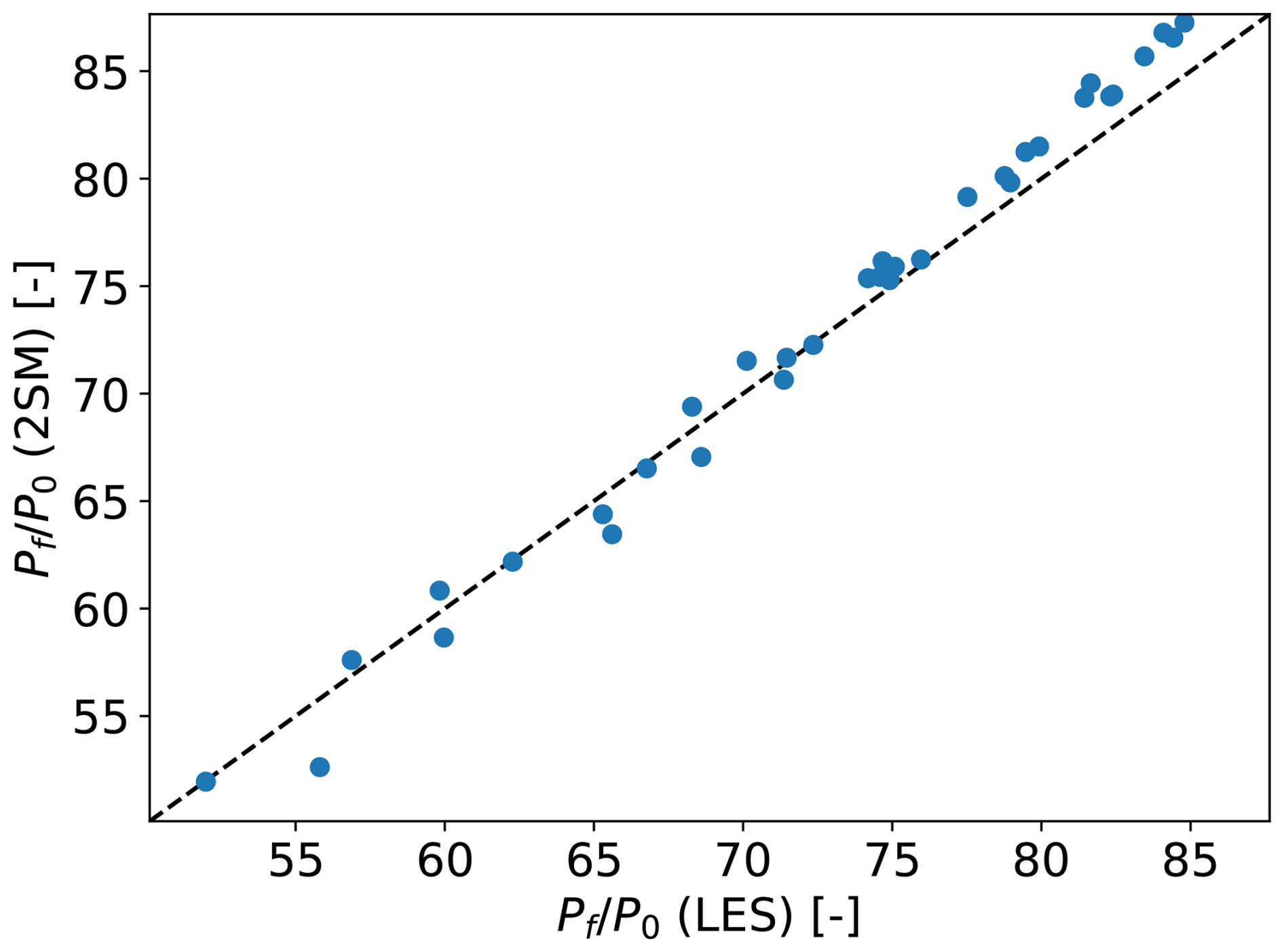
Figure 1A comparison of farm power Pf as calculated by LES (x axis) and Eq. (1) (y axis) for all 36 CNBL cases from the dataset by Lanzilao and Meyers (2024), scaled with the power outputs of standalone turbine simulations P0. The power coefficient is calculated using a neutral flow simulation (i.e., case H500-Δθ0-Γ0 from the same dataset).
If and are known, calculating the farm power output with the 2SM approach then comes down to finding the average farm velocity Uf. The APM is well-suited for this, as it is a fast model for mesoscale atmosphere–farm interaction. Therefore, this section presents a brief overview of the APM.
The APM is a simplified model, and treats the ABL as two layers of vertically averaged flow, separated by a pliant surface following the flow streamlines (Allaerts and Meyers, 2019). In each of these layers, the continuity and horizontal momentum equations are solved explicitly for the average velocities and layer thicknesses. The wind-farm forces are added in the momentum equations for the lower layer, also called the wind-farm layer, while only affecting the upper layer via interactions through the pliant surface. The resulting model structure is visualized in Fig. 2.
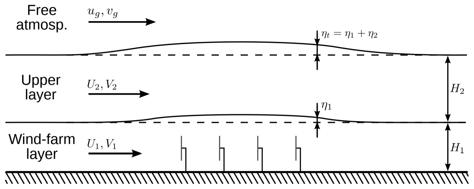
Figure 2Schematic representation of the atmospheric perturbation model. Figure reproduced from Allaerts and Meyers (2019).
The main advantage of the APM is that the vertical averaging drastically lowers the computational cost of the model compared to conventional CFD or mesoscale simulations, since it essentially reduces the vertical resolution to the ABL height. The horizontal resolution is likewise reduced by applying a Gaussian filter with a kernel size of 1 km (Allaerts and Meyers, 2019; Devesse et al., 2024a).
Mathematically, the APM can be derived by applying these filtering and height-averaging operators to the flow. For example, the lower-layer velocity is defined as (Devesse et al., 2024a)
where x, y, and z denote the streamwise, spanwise, and vertical coordinates, respectively, the subscript 1 indicates the lower layer, the angled brackets and tilde denote the height-averaging and filtering, respectively, u is the horizontal velocity vector, h1 is the lower-layer thickness, Lx×Ly is the APM domain size, and Gℓ is a Gaussian kernel with a fixed filter length ℓ=1 km. The pliant surface h1 is defined as following the streamlines of the horizontally filtered flow, so that (Allaerts and Meyers, 2019)
where w is the vertical velocity component and ∇h is the horizontal del operator. The flow is then further linearized around a uniform background state, so that for the lower layer
where U1 and H1 are the unperturbed layer velocity and thickness in the absence of the wind farm and and η1 are the perturbations to this state. For the upper layer, the notation is analogous.
The governing equations of the model can then be found by applying the above operators to the incompressible Reynolds-averaged steady-state Navier–Stokes equations and linearizing the result. Thorough descriptions of this procedure can be found in Allaerts and Meyers (2019) and Devesse et al. (2024a). The resulting set of equations is
where the subscript h indicates horizontal vector components, p′ is the pressure perturbation induced by gravity waves, ρ is the air density, fc is the Coriolis parameter, J is the two-dimensional rotation dyadic, and νt are height-averaged eddy viscosities. Furthermore, Th3,0 and Th3,1 are the unperturbed turbulent shear stresses at the ground and the layer interface, respectively, and C′ and D′ are the Jacobians of these stresses to the layer velocities. Finally, fwf, Δτwf, and 〈τd,hh〉1 are the perturbing effects of the wind farm, with fwf denoting the turbine forces (scaled with air density), Δτwf representing the shear stresses between the layers due to the added turbulence intensity caused by the farm, and 〈τd,hh〉1 denoting dispersive stresses due to turbine-scale flow heterogeneity. For the sake of simplicity, the latter two are not included in this study.
The pressure perturbation in the ABL p′ is caused by the gravity waves on the capping inversion and in the free atmosphere. These waves are themselves triggered by the displacement of the capping inversion . Their pressure feedback can be related to this displacement in Fourier space, so that (Gill, 1982; Smith, 2010)
where g′ is the reduced gravity in the capping inversion, ℱ−1 denotes an inverse Fourier transform, and * denotes a convolution. Continuing, Φ are the stratification coefficients, which determine the pressure feedback of the internal gravity waves in the free atmosphere. For uniform barotropic free atmospheres, these coefficients are calculated in Fourier space as (Allaerts and Meyers, 2019)
where is the Brunt–Väisälä frequency in the free atmosphere and Ω is the intrinsic wave frequency. The vertical wavenumber m is given by the dispersion relation (Smith, 1980):
where the sign of m has to be chosen to ensure that the perturbation dies out with height if m2<0 or that energy radiates outwards if m2>0.
The grid spacing of the APM is significantly larger than the individual turbine diameters. Therefore, the turbine forces are considered to be point forces before they are filtered onto the numerical grid using the same filter as in Eq. (4), so that the total force is simply a sum of Gaussians (Allaerts and Meyers, 2019):
where each Gℓ,k is a Gaussian kernel centered around turbine k, and the turbine thrusts fk are (Allaerts and Meyers, 2019)
where Sk and ek are the turbine disk velocities and orientations, respectively, and can be evaluated using Sk from the turbine thrust coefficient curve. Note that this paper uses the disk-averaged velocities and thrust coefficients, as this simplifies the comparison against LES. In practical application, their free-stream counterparts can also be used, as is commonly done by wake models. Because the APM's resolution is too low to resolve the turbine-scale flow, these quantities are calculated using a wake model. To capture the dependence of the turbine forces on the local mesoscale flow, past studies developed ways to calculate the background velocity used by the wake model based on the APM state (Allaerts and Meyers, 2019; Stipa et al., 2024a; Devesse et al., 2024a, b).
Since the pressure feedback of the internal gravity waves is mostly easily expressed in Fourier space, the system of Eqs. (7)–(11) is solved with a Fourier–Galerkin method. All terms in the equations except the turbine forces then decouple per wavenumber, so that for a given the system can be easily solved through matrix inversion. The turbine forces are included through a fixed-point iteration, where at each step the linear APM equations are solved for a given forcing. The resulting APM state is used to infer a background velocity for the wake model, which is then used to re-calculate the turbine forces fk. This process is repeated until convergence. For details, see Devesse et al. (2024a).
The main numerical costs of the classical APM lie in solving Eqs. (7)–(11) and re-calculating the wake model background velocity at each step of the fixed point iteration (Devesse et al., 2024b). These repeated calculations were needed to resolve the local coupling between the mesoscale APM state and the turbine forces. However, 2SM theory allows us to neglect this local coupling, and consider a farm-averaged approach instead. This is the focus of the following sections.
The 2SM approach simplifies the turbine-scale problem by relating the turbine forces and power outputs to only the average velocity in the farm through and . The most straightforward way of combining this with the APM is then to use the APM as the external model to find Uf, while using and to represent the turbine forces in the APM. This section focuses on developing such coupling and on leveraging the simplifications of 2SM theory to speed up the APM.
The goal of this section is use the APM to solve the external problem as cheaply as possible. Therefore, we treat the farm coefficients and as known inputs for now. However, their computation still represents an additional cost, associated with calculating the farm-averaged velocity in a prior (neutral) wake model simulation. This will be addressed in Sect. 5.2, using insights from the methods developed in this section.
We will build up the combination of the 2SM and APM approaches step by step. First, Sect. 4.1 discusses the differences between the mathematical averaging operators used by 2SM theory and in the derivation of the APM and bridges the gap between them. Then, Sect. 4.2 sets up a simplified version of the APM focused on finding Uf, thereby leveraging the insights of 2SM theory to speed up the model. Sect. 4.3 validates the developed 2SM–APM with the same LES dataset from Lanzilao and Meyers (2024) that was used in Sect. 2. Finally, Sect. 4.4 investigates the use of wake models to calculate and .
4.1 Relating the average APM and 2SM velocities
Combining the 2SM and APM approaches requires us to relate the average farm velocity used in the 2SM equations to the average lower-layer APM velocity within the farm. We defined the former as a straightforward average over the wind farm, so that
where Hf is the height of the 2SM averaging volume and Ωf the planform area of the wind farm. As noted in Sect. 2, modeling wind farms with irregular turbine layouts may require more complex horizontal averaging operators.
In contrast, the APM predicts a horizontally filtered, height-averaged velocity field:
Averaging the APM variables over the farm can therefore only be done horizontally, so that
where the bars indicate horizontally averaging over the farm.
Clearly, the averages defined by Eqs. (3) and (16) are not equivalent. Since the internal 2SM problem has to remain constant, the volume over which the farm average is defined should be independent of the mesoscale perturbation. However, the layer interface in the APM follows the flow streamlines, and its vertical displacement η1 is part of the model state. This results in two different control volumes, as sketched in Fig. 3. Moreover, the APM velocity is filtered horizontally before being averaged, while the 2SM velocity is not.
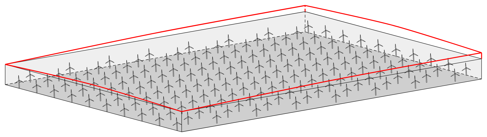
Figure 3Sketch of the farm control volume (black) and lower APM layer (red) for a rectangular farm. Note that in contrast to the 2SM farm control volume, the upper boundary of the APM layer is not rigid, as it follows the streamlines.
In this work, we neglect the filtering effects, thus presuming
Relating the 2SM and APM averages then only requires accounting for the discrepancy in the control volumes. Choosing Hf=H1 makes these volumes as similar as possible, so that the remaining difference is solely due to the streamline displacement η1. The velocity in this region depends on the relative strength of the turbulent entrainment and gravity-wave-induced pressure gradients. Here, we take the simplest possible approach by assuming that the average velocity perturbation in the part of the APM layer above the 2SM volume scales with the velocity deficit within it, so that
where U0 is the unperturbed velocity profile, α is a tuning parameter between 0 (no velocity deficit in the region ) and 1 (perfectly mixed APM layer), and is the 2SM-farm-averaged velocity deficit:
Taking the vertical integral up to , we then find
The 2SM-farm-averaged velocity can then be calculated from the APM state as
We tune α using the NBL case H500-Δθ0-Γ0 from the dataset of Lanzilao and Meyers (2024). We calculate the APM state (, η1) directly from the LES data by horizontally filtering the time-averaged flow field, advecting a set of points to find the displacement of the APM layer η1, and height-averaging the flow. A detailed description of this procedure can be found in Devesse et al. (2024a). By relating the LES-based APM state set up this way to the Uf calculated directly from the LES using Eq. (3), we find α=0.16. Note that this basic approach does not capture the significant differences in velocity profiles between NBL, CNBL, and realistic flows, or the effects of wind farm layout and thrust distribution. Instead, it is chosen for its simplicity.
4.2 Basic 2SM–APM coupling
We now focus on a fast 2SM–APM variant that will require solving the APM Eqs. (7)–(11) only once, rather than at every iteration, thereby significantly speeding up the model.
We begin by simplifying the notation. We can write the APM as a set of linear operators that transform the turbine forces to an APM state, so that
where 𝒜u, 𝒜η, and 𝒜p are linear operators that follow from the APM Eqs. (7)–(11) and fwf is the turbine force. Note that this assumes that the direct turbine forces are the only perturbing forcing in the ABL. A more general approach would have to include the dispersive stresses and the increase in momentum flux as well. A discussion on such an extension is given at the end of this section.
When using the APM with conventional wake model coupling methods, one of the largest computational costs is applying these operators 𝒜, which involves a large linear system solve, at each step of the fixed-point iteration (Devesse et al., 2024b). In the classical APM, this iteration is needed because at each point in space, the local height-averaged farm force depends on the local velocity and layer thickness. While these local values impact individual turbine performance, they are not relevant to the 2SM approach, as it only requires the average velocity over the farm to calculate the farm power output. Since the goal of the 2SM–APM is to compute this farm-averaged velocity as cheaply as possible, including local variations is an unnecessary cost. Therefore, we will assume that the distribution of the force in space, normalized by the total force , is independent of the APM state , so that
where Πf is the geometric footprint of the height-averaged force, and F is the total farm thrust (see Eq. 2). If this footprint is indeed independent of the APM state, the model is reduced to a set of scalar equations:
where the coefficients au and aη can be pre-computed:
We then arrive at a closed system of equations by computing the farm force F with Eq. (2), while relating Uf to the average APM perturbations using Eq. (21):
The linear system of Eqs. (7)–(11) now has to be inverted only once when calculating au and aη. This effectively reduces the cost of the model to a single step of the fixed-point iteration used by the classical APM while still incorporating the overall feedback between the total farm force and the blockage effects.
The closer the footprint Πf is to the actual normalized force distribution, the more accurate we expect the coefficients au and aη to be. However, this actual footprint is not known a priori. Instead, we use a standalone wake model to estimate the footprint cheaply. The wake model can predict the turbine disk velocities Sk, which can be combined with Eqs. (14)–(15) to find the farm forcing, so that
where the subscript WM indicates the variables are calculated using a standalone wake model. This approximates the footprint of a farm in neutral conditions at a low computational cost.
We briefly discuss how this 2SM–APM coupling relates to the coupling methods between the APM and underlying wake models developed in previous work. The most similar conventional method is the velocity matching (VM) approach developed by Devesse et al. (2024a), which calculates a background velocity that ensures that the wake model and the APM predict the same mesoscale velocity field at each point in the farm. This 2SM coupling imposes the same condition but only on a farm average, so that the average farm velocity is the same in the internal and external problems (Nishino and Dunstan, 2020). Therefore, the 2SM–APM coupling can be seen as the VM method with just one degree of freedom for the background velocity.
Including additional wind-farm perturbing forces, such as the induced dispersive and turbulent stresses, can be done by following the same steps as above. Since the APM operators are linear, the responses to different inputs can simply be summed up. If the perturbing forces scale with , as can be assumed for the dispersive stresses, this results in a modification of Πf when calculating au and aη. However, including perturbing forces that scale differently, like the turbulent momentum flux in the upper layer, requires calculating additional coefficients for the scalar system of equations. We leave these complications to future work.
4.3 Comparison to LES
To test the 2SM–APM approach, we validate the model with the CNBL LES results of Lanzilao and Meyers (2024) that were used in Sect. 2. Like before, the farm coefficients are calculated using the neutral H500-C0-G0 case, which results in and . This ensures that any errors introduced will come from the 2SM–APM coupling and not from the estimation of the farm coefficients. The unperturbed background APM state is based on the precursor simulation driving each of the wind-farm simulations. We leave out the H150 cases, since the three-layer APM can not handle very shallow upper-layer heights H2 for the time being (Devesse et al., 2024a).
The numerical setup is the same as described in Devesse et al. (2024a). As discussed in the previous section, the APM operators 𝒜 are solved using a Fourier–Galerkin method. To prevent the perturbations recycling through the periodic boundaries imposed by this method, we use the very large domain length of Lx=10 000 km in the streamwise direction. In the spanwise direction, we take Ly=30 km in order to follow the LES results as closely as possible. The grid resolution is half of the horizontal filter length, so that m.
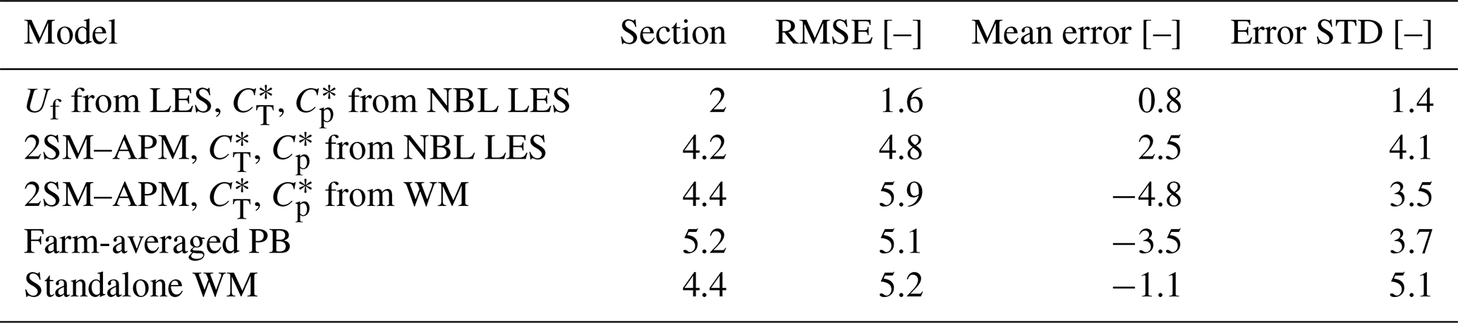
The resulting predictions for the farm power Pf are shown in Figs. 4 and 5, and the corresponding error statistics are listed in Table 2. The fast 2SM–APM seems to perform well overall, with the general trend being clearly visible. The root-mean square error (RMSE) across all analyzed cases is 4.8P0 (where P0 is the power output of an isolated turbine), or 3 % of the farm's installed capacity. As shown in Table 2, this RMSE is mostly due to the variance in the model errors, as the mean bias is comparatively small. Looking at Fig. 5, there seems to be no consistent relation between the model error and the varying atmospheric parameters H, ΔΘ, or Γ. Instead, Fig. 4 shows that there is a small but consistent positive bias and that the scatter on the model's predictions is larger at lower farm power outputs, i.e., for cases with stronger blockage effects.
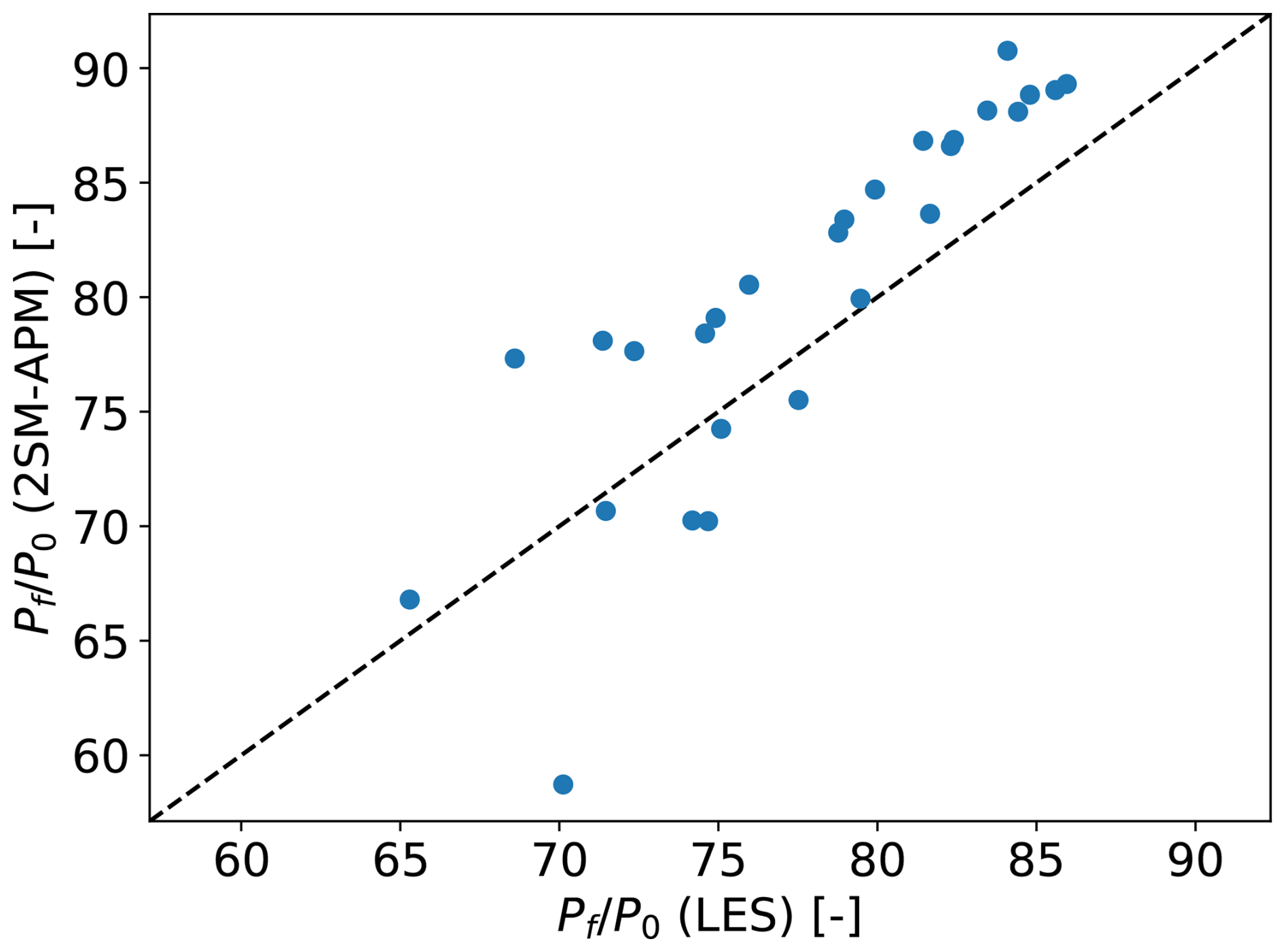
Figure 4A comparison of farm power Pf as calculated by LES and the fast 2SM–APM model for 27 different CNBL cases from Lanzilao and Meyers (2024). The footprint of the height-averaged turbine forces is assumed to be constant, so that the linear system of APM equations only has to be solved once. The axes are normalized with the power output of a standalone turbine P0.
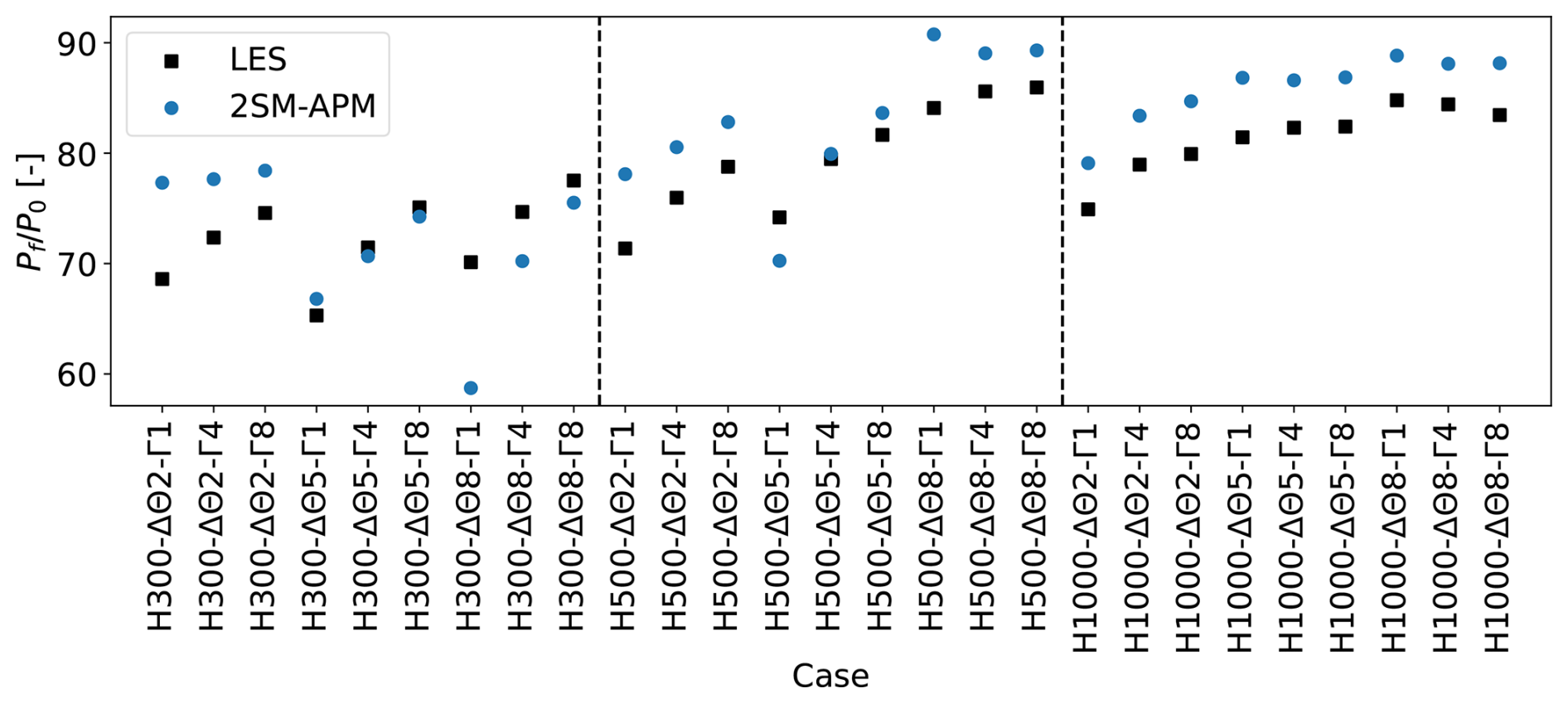
Figure 5The farm power Pf as calculated by LES (black, □) and the fast 2SM–APM model (blue, ∘) for the different cases from the dataset by Lanzilao and Meyers (2024). All values are normalized by the power output of a standalone turbine P0. The dashed lines separate the cases with different ABL heights.
Table 2The root-mean square (RMSE), mean, and standard deviation (STD) of the error of farm power Pf of all the models analyzed in the current paper for the LES dataset from Lanzilao and Meyers (2024). The “Section” column lists which sections of the paper describe the various models. All values are scaled with the power output of a standalone turbine. Note that the three error metrics are related, as .
To investigate the model's performance further, Fig. 6 shows velocity deficits as predicted by the fast 2SM–APM model for three different cases, and compares them to the LES results. The three cases are H500-Δθ5-Γ4 (left), H1000-Δθ2-Γ1 (middle), and H300-Δθ8-Γ1 (right), which are the cases where the model performs best, median, and worst, respectively. In general, accurate predictions of the average velocity are in part due to a cancellation of errors, as the model over- and underpredicts the velocity at the front and back of the farm, respectively. While the model predicts the wrong location for the resonant lee waves for some of the H300 cases, as can be seen in Fig. 6 (right), this is not a consistent source of error. These errors in the local velocity profiles are not due to the 2SM simplifications, as earlier conventional versions of the APM have similar behavior (Devesse et al., 2024a).
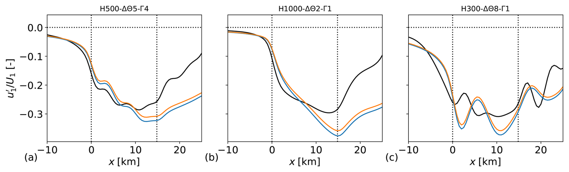
Figure 6Lower-layer velocity deficit through the center of the farm as predicted by LES (black) and the fast 2SM–APM (blue, orange) for the cases H500-Δθ5-Γ4 (left), H1000-Δθ2-Γ1 (middle), and H300-Δθ8-Γ1 (right). The dotted lines denote the wind farm region. The blue and orange lines showing the 2SM–APM predictions were obtained with values calculated using LES and a wake model, respectively.
Lastly, we discuss the computational cost of the 2SM–APM. As desired, the model achieves a relatively low computational cost, with each calculation taking roughly 1.3 CPU seconds on an Intel Xeon Platinum 8360Y 2.4 GHz CPU. This is only approximately 35 times longer than a wake model evaluation for the same farm, and drastically faster than the conventional APM with local coupling (Devesse et al., 2024b). The main computational gains are achieved by eliminating the costs of re-calculating the turbine forces and of repeatedly solving the APM Eqs. (7)–(11). While the former cost is shifted to the calculation of the farm coefficients and , as discussed in the next section, the latter is fully removed.
4.4 Using a wake model to compute and
When using the 2SM–APM in practical settings, it is not feasible to rely on LES to calculate the farm thrust and power coefficients and , as these simulations are too expensive. Therefore, this section aims to briefly demonstrate how a basic wake model can be used to calculate these coefficients instead of LES. We merely wish to show that this approach is conceptually possible and point out some potential issues.
In essence, the process is the same as before, i.e., the standalone wake model is used to estimate Uf, Pf, and F for a given farm, so that and can be calculated using Eqs. (1) and (2). As shown in Sect. 2, the resulting coefficients capture the turbine-scale flow characteristics and are valid across a range of atmospheric conditions as long as the turbine setpoints and wake shapes remain the same. Once they are calculated, the 2SM–APM can use them to predict the farm power output in different mesoscale flow conditions.
To calculate the farm power and thrust, we use a Gaussian wake model (Bastankhah and Porté-Agel, 2014) with the wake merging method of Lanzilao and Meyers (2021) and the turbulence-intensity model of Niayifar and Porté-Agel (2016). The wake model is not tuned and is run with the parameters reported by the above authors. The turbines are mirrored to account for ground effects, as this significantly reduces the error of the predicted power output and farm-averaged velocity. This conflicts with the results from Bastankhah and Porté-Agel (2014), who found that mirroring the turbines had little effect on the WM's predictions. This difference with the original papers might be because we use a turbine type with a higher ratio of , leading to the rotors being relatively closer to the ground.
Accurately calculating Uf with a wake model requires more modeling effort than Pf and F (Devesse et al., 2024a). Since wake models typically only need to estimate the velocity at downstream turbine locations, they are not always optimized for velocity estimations in the near-wake and induction regions. If not properly accounted for, this can lead to large errors in the average velocity predictions. Therefore, we follow Devesse et al. (2024a) and include a turbine-induction model when estimating Uf (Troldborg and Meyer Forsting, 2017).
The farm-averaged velocity Uf is calculated by evaluating the wake model on a dense, evenly spaced grid over the whole 2SM averaging volume. This brute-force approach is computationally expensive, and a more efficient placement of the evaluation points would likely improve it. However, as this section simply aims to demonstrate that this type of wake model coupling can be done in principle, we leave further optimizations of how to estimate Uf to future work.
The resulting and are 1.05 and 0.79, respectively. Both values are lower than those calculated from the neutral LES (1.15 and 0.92). This is mostly due to an error in Uf, as even with an induction model, the farm-averaged velocity is overestimated (Devesse et al., 2024a).
With these coefficients, we now repeat the earlier validation using the LES dataset from Lanzilao and Meyers (2024). Figure 7 and Table 2 show the resulting farm power predictions and error statistics, respectively, for both the 2SM–APM and the standalone wake model. Using the wake model to calculate and leads to a higher errors, mainly due to the consistent negative bias. Interestingly, the standalone wake model has a similar RMSE as the 2SM–APM despite not capturing any of the power variations in the dataset, mostly because its mean error is very small. In comparison, the 2SM–APM have a higher bias but a significantly lower variance.
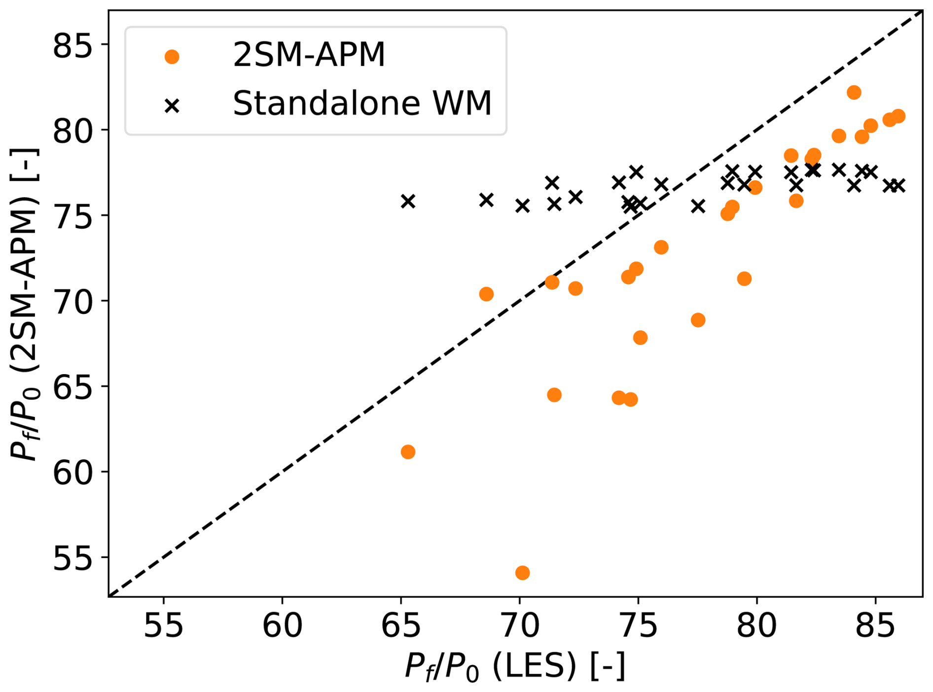
Figure 7A comparison of farm power Pf as calculated by LES (x axis), the fast 2SM–APM model (orange circles), and a standalone wake model (black crosses) for 27 different CNBL cases from Lanzilao and Meyers (2024). The farm coefficients and used by the 2AM–APM are calculated using the wake model. The axes are normalized with the power output of a standalone turbine P0, as calculated using LES (horizontal) and the wake model (vertical).
To investigate further, Fig. 6 shows the velocity perturbations predicted by the 2SM–APM. As a result of the lower value, the model predicts smaller than before, leading to higher Uf. However, this is counteracted by the lower , so that the resulting farm power predictions have a consistent negative bias.
The above discussion shows that in principle wake models can serve the role of a prior CFD simulation in determining and but that this requires the wake model to accurately represent the flow in the induction and near-wake regions. The associated computational cost can be significantly reduced by future research, as we have made no attempts to minimize it. Furthermore, constructing lookup tables for and as a function of wind speed and wake model inputs would allow this upfront cost to be shared by many 2SM–APM cases when performing multiyear AEP estimates, among other things. Finally, the coefficients could potentially also be inferred directly from operational data. Instead of investigating these approaches further, the following section develops a second version of the 2SM–APM which is directly coupled to a wake model, eliminating the need for an explicit calculation of and .
The previous section treated and as known inputs from a prior simulation or wake model and focused on improving the APM's cost and performance. However, calculating these coefficients with a wake model places requirements on said wake model's performance and comes at a potentially significant computational cost. Therefore, we now apply the constant-footprint technique developed in the previous section to the pressure-based (PB) wake model coupling developed by Stipa et al. (2024a), resulting in a blockage-corrected model for farm power that does not require the explicit calculation of and .
This section first briefly derives the pressure-based wake model coupling technique. Afterwards, it applies the techniques developed in the previous section to eliminate the repeated APM operators. The resulting model is again validated using the CNBL simulations of Lanzilao and Meyers (2024).
5.1 Derivation of the pressure-based coupling method
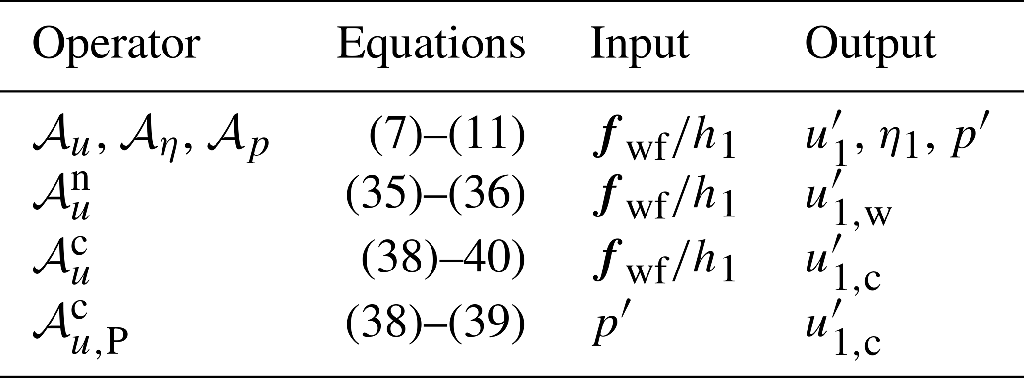
This section derives the equations for the pressure-based coupling method developed by Stipa et al. (2024a), by interpreting the APM as a correction model for CNBL effects. A similar but less thorough derivation has been made before by Devesse et al. (2024b). A graphical representation of the coupling and the derivation is given in Fig. 8, and an overview of the shorthand notations for the different operators used is given in Table 3.
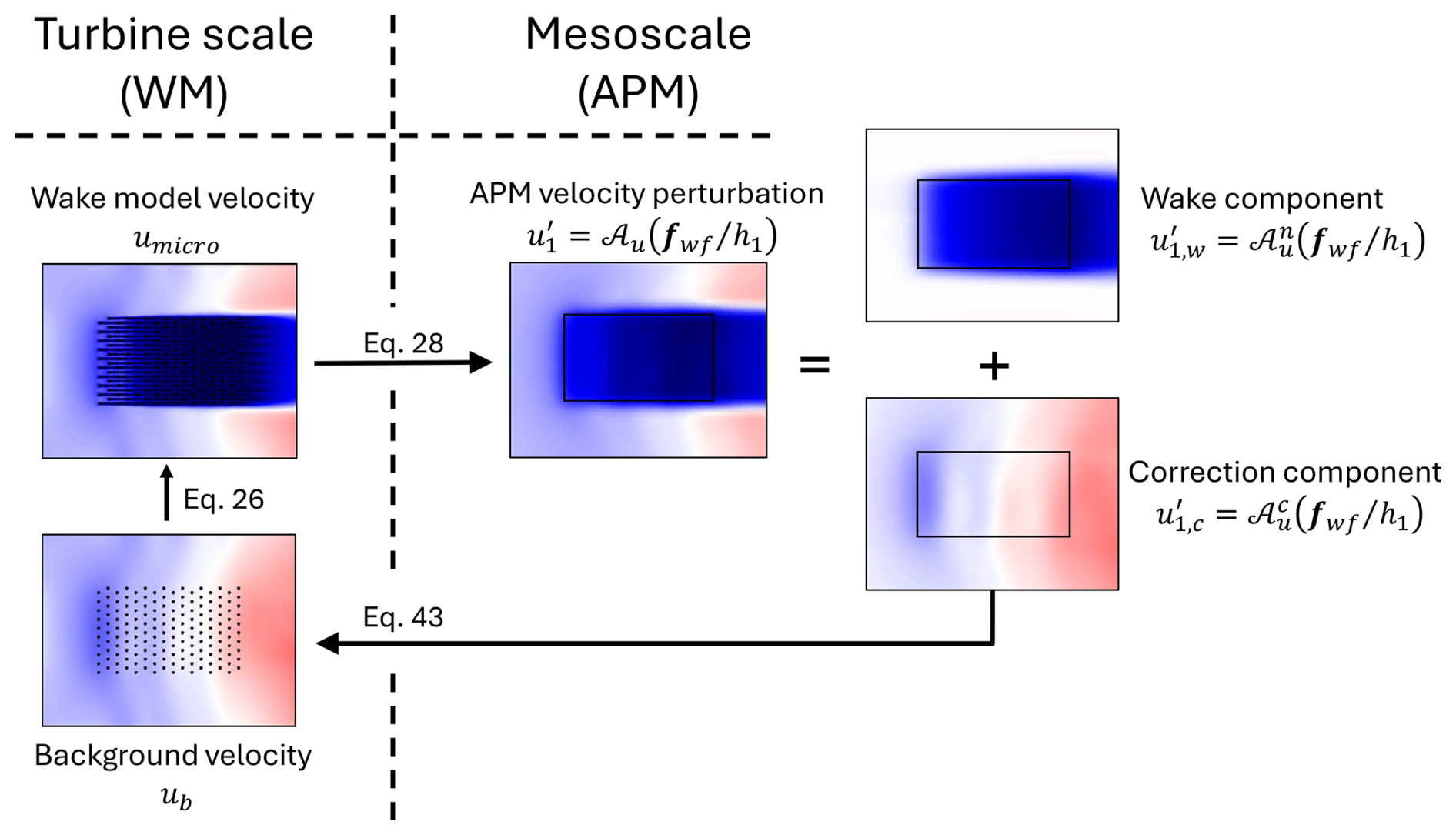
Figure 8A conceptual sketch of the pressure-based coupling method. We argue that the APM velocity perturbation can be split up into wake and pressure components and that the latter can serve as the change in background velocity for the wake model due to blockage and gravity-wave effects. Figure based on Stipa et al. (2024a).
Table 3Overview of the shorthand notations for the different operators used in this paper, the sets of equations they represent, and the variables that serve as their in- and outputs.
A wake model estimates the turbine-scale velocity field umicro by superposing turbine wake functions on a given background velocity Ub, so that
where WM is the wake model operator.
The background velocity Ub is defined as being the velocity field that will result in the correct umicro when the wakes are superimposed on it. In the absence of blockage and gravity-wave effects, this is simply the unperturbed velocity in the absence of the wind farm, so that . In contrast, when coupling a wake model to the APM, Ub has to ensure that horizontally filtering and height-averaging the turbine-scale velocity field results in the APM velocity, so that
Devesse et al. (2024a) call this the velocity matching (VM) equation. This condition gives an implicit equation for Ub and is related to using the pre-computed farm coefficients and when simplifying the APM–WM coupling using two-scale momentum theory, as discussed in the previous section. Similar to computing these farm coefficients, solving the VM equation for Ub is relatively expensive (Devesse et al., 2024b).
In order to find a computationally cheaper way to estimate Ub, we decompose the filtered, height-averaged wake model operator into a wake and a correction component, so that
where the wake component is the filtered and height-averaged velocity deficit corresponding to the turbine wakes, as predicted by the wake model, and the correction component accounts for the remainder of the total velocity perturbation . This splitting is shown conceptually on the right-hand side of Fig. 8. For sufficiently small flow perturbations, we can then assume that subtracting the wake component from the above equation corresponds to not applying the wake model operator WM, so that
We can therefore interpret the correction component as representing the changes in the background velocity that we are trying to estimate.
Instead of deriving an expression for directly, we will derive it as the difference between the APM state and the wake component . Using Eq. (28), we find
Therefore, the next step is to estimate , i.e., the part of the APM velocity perturbation that corresponds to the wake deficit predicted by the wake model. Rather than obtaining this by averaging over the microscale velocity predicted by the wake model, we aim at finding an APM operator that allows us to make a faster direct estimation of . Since conventional standalone wake models are designed to estimate the response of a neutral atmosphere to turbine forcing, we can reasonably take
where is the APM operator for neutral conditions. The component can then be seen as a correction to neutral flow due to blockage effects and is defined as
where is the APM operator for the difference between CNBL and neutral flow:
If this correction operator is known, it can be used to directly predict (and correspondingly Ub), without explicitly solving the velocity matching equation. To find , we first construct the neutral APM operator , since they are related through the above equation.
To find the neutral APM operator , we re-derive the APM for neutral flow. Doing so, the continuity and momentum equations remain unaltered. The only equation that changes is the pressure closure equation. In the absence of gravity waves, the pressure perturbations triggered by the farm are solely due to hydrodynamic effects, which are small compared to the buoyancy effects at typical wind farm length scales. This is demonstrated by the LES data of Lanzilao and Meyers (2024), where the pressure perturbations in the neutral cases are negligible compared to the CNBL simulations. Therefore, we take .
We then easily find the model for the neutral component as Eqs. (7)–(11) without the pressure term. For the sake of brevity, we only write the equations for the lower layer:
The equations for the correction operator can then be found by simply subtracting the above equations for the neutral model from the original APM continuity and momentum equations. Doing this results in
where we again only write the lower-layer equations for the sake of brevity. Note that for a given forcing , the pressure perturbation p′ follows from Eq. (22) (based on the original APM operator 𝒜p) and is an input to Eqs. (38)–(39).
We again define a simplified notation that expresses as the solution of the above system of equations:
where the operator represents the solution operator of Eqs. (38)–(39) given p′ as an input. Note that thus defines (Eq. 34).
Finally, we have thus arrived at a closed system of equations, as through Eq. (41) we can calculate the change in background velocity for a given forcing . This allows us to again employ a fixed-point iteration, where fwf is calculated using the wake model, and the corresponding changes in h1 and u1,c are calculated using 𝒜η and , respectively. The wake model then re-calculates the forces with the updated background velocity. This process is repeated until convergence.
The only remaining issue is that the input to the wake model requires a turbine-scale background velocity that is not height-averaged. The pressure-based coupling method therefore constructs a local background velocity for the wake model based on (Stipa et al., 2024a). Following the linearization of the APM, we write this background velocity Ub as the sum of the unperturbed velocity profile in the absence of the farm U0 and a perturbation around it, so that
where 〈U0〉1=U1, and fb is a shape function (we typically choose a logarithmic function). The perturbation to the background velocity is then found by matching the height-averaged , so that
Stipa et al. (2024a) did not include the background component of the continuity equations (Eq. 38) in their original coupling. However, the above derivation of the method shows that the whole APM operator should be split. These continuity equations add a parabolic behavior to the correction operator , so that the periodic boundary conditions imposed by the Fourier–Galerkin spectral method used to solve the original APM equations become inappropriate. However, since the closure equation for the internal gravity waves (Eqs. 11–12) is not a part of the correction operator, we are free to use other numerical methods. Therefore, we solve Eqs. (38)–(39) with a simple first-order explicit Euler marching scheme, with as inlet boundary conditions , which correspond to there being no pressure-induced change in background velocity at the inlet. For these conditions to be valid, the inlet should be placed far enough upstream of the farm so that , which for realistic atmospheric conditions is typically less than 100 km (Smith, 2024). As a result, the operator can use far smaller grid sizes than the periodic boundary conditions required of the conventional APM. Finally, in order to simplify the marching solver, we neglect the horizontal eddy viscosity, so that there are no second-order derivatives in the equations.
5.2 Farm-level pressure-based APM–WM coupling
We now apply the farm-averaging approach developed in the previous section to the PB coupling method. As discussed above, the background component of the APM velocity perturbation is given by
By plugging in the constant footprint (Eq. 23), we find that the average streamwise correction component is
where the coefficient can be calculated as
The average layer displacement can be found through Eq. (24), as in the basic 2SM–APM.
Following the pressure-based coupling approach, we now use this to directly correct the background wind speed in a wake model. Since the above results only hold on a farm average, we assume a constant background over the farm:
where the average background velocity scale is found by matching :
The wake model can then be used to calculate F and Pf, closing the system of equations:
where the turbine coefficients and disk velocities are calculated using a wake model with the background velocity defined in Eq. (46).
We solve the final system of Eqs. (44), (24), (48), (49) using a fixed-point iteration solver with a relaxation factor of 0.7, as is done for the classical APM and the 2SM–APM developed in the previous section.
The advantages of this approach compared to the 2SM–APM coupling derived in the previous section are similar to the advantages of PB coupling compared to the VM method. It places no requirements on the wake model and does not need to calculate and . Its main disadvantage is that it requires an additional solver for the operator , corresponding to Eqs. (38)–(39). However, since it can use a simple first-order marching scheme and a relatively small grid, this solver is straightforward to implement and cheap to run. Finally, we emphasize that while this coupling no longer explicitly uses any of the results from 2SM theory, it implicitly makes the same assumption that farm power calculations only need the average wind speed within a farm.
Comparison to LES
We again validate this approach using the LES cases from the dataset by Lanzilao and Meyers (2024) used throughout this work. The numerical setup for the 𝒜p operator is the same as in Sect. 4.3. The correction operator can use a smaller numerical domain, since its solver does not require periodic boundary conditions. Here, we use the same spanwise Ly=30 km as before but take a shorter streamwise Lx=43 km, placing the solver's inlet at the same upstream distance of the farm as the LES, i.e., 18 km. We use the same wake model as in Sect. 4.4.
The results are shown in Fig. 9, and the error statistics are listed in Table 2. The general trend is visible, despite some scatter and a consistent negative bias. Overall, the wake model and the farm-level PB coupled model have the same RMSE for a power of 5.1P0, or 3.2 % of the farm's installed capacity, with the farm-averaged PB model having a lower error variance but larger bias. The computational cost is the same as before, as the pressure component operator and wake model evaluations have a negligible cost.
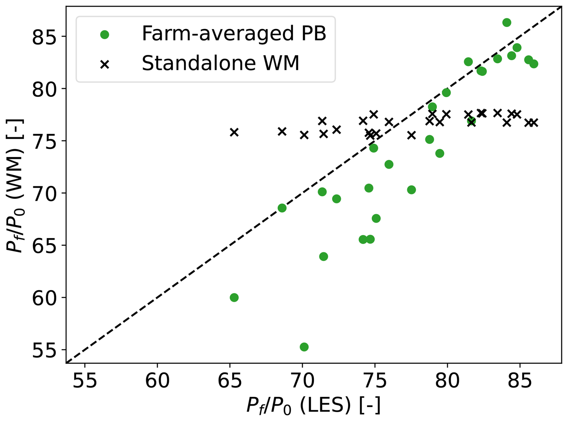
Figure 9Farm power as calculated by LES (x axis) and wake model (y axis), both standalone (black crosses) and with farm-average pressure-based blockage coupling (green circles). The axes are normalized with the power output of a standalone turbine P0, as calculated using LES (horizontal) and the wake model (vertical).
As shown above, the pressure-based coupling can be derived as a correction to an NBL base state. With that in mind, Fig. 10 shows the difference in farm power between the coupled and standalone wake model, compared to the farm power differences between the CNBL and the neutral LES reference simulation, i.e., H500-Δθ0-Γ0. It is clear that the farm-average coupling performs decently in the role of a blockage-correction model, as it captures the overall trend despite a consistent bias. The error of this power difference is similar to the error of the farm powers shown in Fig. 9, which indicates that the farm-averaged PB model's bias is mostly due to an overprediction of blockage losses.
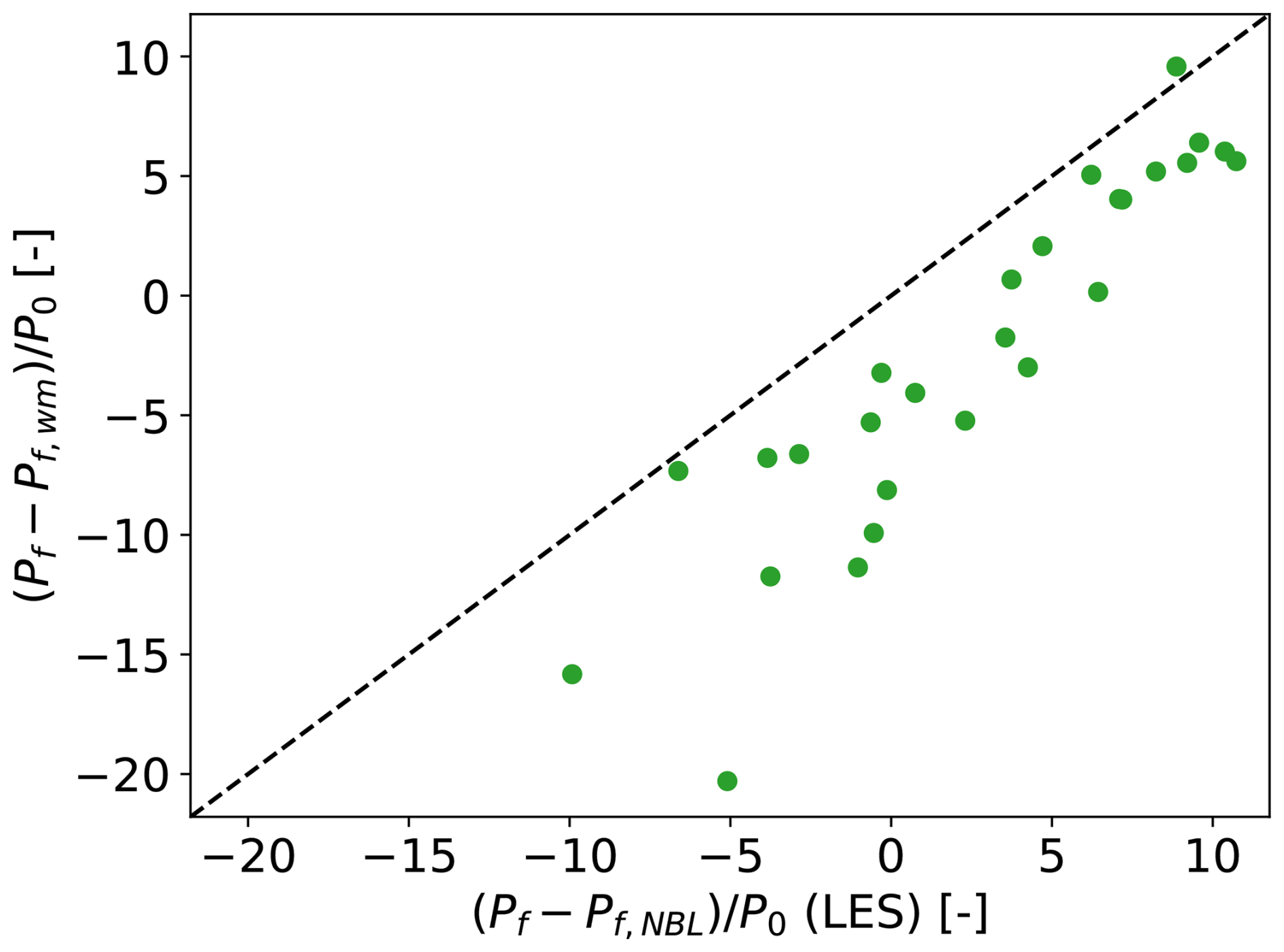
Figure 10Difference between farm power in CNBL and NBL conditions as calculated by LES (x axis) and wake model with farm-average pressure-based blockage coupling (y axis). The axes are normalized with the power output of a standalone turbine P0, as calculated using LES (horizontal) and the wake model (vertical).
This section gives a brief overview and comparison of the performance of the models developed in the previous sections. We emphasize that these conclusions are drawn based on a validation campaign using idealized LES results and that more work is needed to investigate both the 2SM hypothesis and the models' performance further using real operational data.
When validated with the idealized LES results from Lanzilao and Meyers (2024), both the -based 2SM–APM and the farm-averaged PB method perform similarly well. When compared to a standalone wake model, they have the same RMSEs on power output of 3 % to 4 % of the farm's installed capacity, as summarized in Table 2. They can better capture the spread in the dataset due to blockage effects but have a larger bias in their power predictions. Their computational cost is 35 times higher than that of the wake model but still orders of magnitude below conventional CFD or APM tools.
The coefficient-based 2SM–APM represents the farm using pre-defined and coefficients. Because of this simplicity, it has the advantage of only needing to solve one set of equations. Furthermore, if the farm power and thrust coefficients are known accurately, it has the lowest RMSE out of all the models tested. However, these coefficients, along with the tuned parameter α, are not trivial to estimate. Its applicability is therefore partially dependent on future work developing methods for calculating the and of real wind farms. Progress on estimating these coefficients would also benefit actuator-farm and mesoscale weather models (van der Laan et al., 2023; Du et al., 2025).
The farm-averaged PB method captures turbine-scale effects through repeated wake model evaluations. As shown in the previous section, this can be interpreted as correcting neutral-flow results for gravity-wave effects. This approach avoids the need for pre-calculating farm coefficients, making it easier to set up for different farm layouts and operating setpoints. However, it comes at the cost of having to solve an extra set of equations.
Two-scale momentum (2SM) theory offers a new way of including mesoscale effects in wind farm power predictions. Using results from Lanzilao and Meyers (2024), its core hypothesis of scale separation between the turbine- and farm-scale flows was validated for steady-state idealized CNBL conditions. Building on that, this paper developed two ways to combine it with an atmospheric perturbation model (APM) to speed up farm power calculations. This speed-up is possible because according to the 2SM hypothesis, only the average velocity within a farm Uf is needed to compute the farm's force and power output. Since local fluctuations in the turbine forcing are therefore not relevant, the spatial distribution of the forces is assumed to be constant and independent of the APM state. Combined with the linearity of the APM, this transforms the APM's governing equations into a system of algebraic equations, which are trivial to solve numerically.
The first version of the 2SM–APM uses the APM as a mesoscale model to obtain the average velocity within the farm, and uses the 2SM farm coefficients and to calculate the turbine forces and power output. This basic coupling method is similar to the velocity matching method developed in by Devesse et al. (2024a), as it matches the average farm velocity between the meso- and turbine scales. In a validation campaign using the LES results from Lanzilao and Meyers (2024), its RMSE on farm power was only 3 % of the installed capacity when using LES-based values for and . Furthermore, we addressed the model's reliance on accurately knowing these coefficients by showing how they could in principle be calculated using a standard wake model.
The second model developed in this paper avoids the explicit use of and by coupling directly to a wake model. To this end, it applies the farm-averaging approach to the pressure-based wake model coupling method of Stipa et al. (2024a). Based on a rigorous derivation of this method, we show that it can also be interpreted as a model to correct neutral flow results for CNBL effects. The model performs similarly to the first model and can predict the effects of blockage and gravity waves on farm power, albeit with a consistent bias.
Both the 2SM–APM model and the farm-averaged pressure-based approach have a similar accuracy and computational cost. Which of them is preferable largely depends on the trade-off between efficiently calculating the farm coefficients and for the former and solving additional equations for the latter. This investigation is left as future work.
Both models achieve a lower variance in the error of their power predictions compared to a standalone wake model, at the cost of introducing a larger bias. Tuning the underlying wake models could compensate for this, as both the wake spreading coefficients and the farm power and thrust coefficients and can be modified. The low computational cost of the models allows this tuning to directly incorporate large operational datasets. We believe this is a promising area of further research that will facilitate the model's adoption by the wind energy industry and community.
As powerful as the tools offered by the 2SM approach are, it remains unclear how valid the underlying assumptions are outside of the idealized conditions they have been tested in. So far, they have only been validated using LES of infinite farms (Kirby et al., 2022) and farms operating in horizontally homogeneous background conditions with uniform turbine layouts and constant thrust coefficients (Kirby et al., 2025). Future work should investigate whether the farm coefficients remain constant under realistic and transient atmospheric conditions and how to account for irregular turbine spacing and operating setpoints.
The models developed in this paper have been implemented in the open-source code WAYVE https://doi.org/10.48804/XMNVVY (Devesse et al., 2023).
All data used in this paper is publicly available. The LES data can be found at https://doi.org/10.48804/L45LTT (Lanzilao and Meyers, 2023b). Additionally, a repository containing post-processed data to be used directly as input for WAYVE can be found at https://doi.org/10.48804/WL73U5 (Devesse and Meyers, 2026).
KD and JM jointly derived the 2SM–APM couplings and set up the validation studies. KD performed code implementations and carried out the simulations. KD and JM jointly wrote the article.
At least one of the (co-)authors is a member of the editorial board of Wind Energy Science. The peer-review process was guided by an independent editor, and the authors also have no other competing interests to declare.
Publisher's note: Copernicus Publications remains neutral with regard to jurisdictional claims made in the text, published maps, institutional affiliations, or any other geographical representation in this paper. The authors bear the ultimate responsibility for providing appropriate place names. Views expressed in the text are those of the authors and do not necessarily reflect the views of the publisher.
The authors thank Frederik Aerts for insightful discussions on combining the 2SM and APM approaches.
This research has been supported by the Energy Transition Fund of the Belgian Federal Public Service for Economy, SMEs, and Energy (FOD Economie, K.M.O., Middenstand en Energie), by the European Union Horizon Europe Framework programme (HORIZON-CL5-2021-D3-03-04) (grant no. 101084205), and by Project Cloud4Wake, funded by Vlaamse Agentschap Innoveren & Ondernemen (VLAIO) under the Blue Cluster cSBO programme (grant no. HBC.2022.0549).
This paper was edited by Sandrine Aubrun and reviewed by three anonymous referees.
Allaerts, D. and Meyers, J.: Boundary-layer development and gravity waves in conventionally neutral wind farms, J. Fluid Mech., 814, 95–130, https://doi.org/10.1017/jfm.2017.11, 2017. a
Allaerts, D. and Meyers, J.: Gravity Waves and Wind-Farm Efficiency in Neutral and Stable Conditions, Bound.-Lay. Meteorol., 166, 269–299, https://doi.org/10.1007/s10546-017-0307-5, 2018. a
Allaerts, D. and Meyers, J.: Sensitivity and feedback of wind-farm-induced gravity waves, J. Fluid Mech., 862, 990–1028, https://doi.org/10.1017/jfm.2018.969, 2019. a, b, c, d, e, f, g, h, i, j
Bastankhah, M. and Porté-Agel, F.: A new analytical model for wind-turbine wakes, Renew. Energ., 70, 116–123, https://doi.org/10.1016/j.renene.2014.01.002, 2014. a, b
Bleeg, J., Purcell, M., Ruisi, R., and Traiger, E.: Wind farm blockage and the consequences of neglecting its impact on energy production, Energies, 11, https://doi.org/10.3390/en11061609, 2018. a
Centurelli, G., Vollmer, L., Schmidt, J., Dörenkämper, M., Schröder, M., Lukassen, L. J., and Peinke, J.: Evaluating Global Blockage engineering parametrizations with LES, J. Phys. Conf. Ser., 1934, 012021, https://doi.org/10.1088/1742-6596/1934/1/012021, 2021. a
Devesse, K., Lanzilao, L., Allaerts, D., Jamaer, S., and Meyers, J.: Wind-fArm gravitY-waVe and blockagE code, GitLab [code], https://doi.org/10.48804/XMNVVY, 2023. a
Devesse, K., Lanzilao, L., and Meyers, J.: A meso–micro atmospheric perturbation model for wind farm blockage, J. Fluid Mech., 998, A63, https://doi.org/10.1017/jfm.2024.868, 2024a. a, b, c, d, e, f, g, h, i, j, k, l, m, n, o, p
Devesse, K., Stipa, S., Brinkerhoff, J., Allaerts, D., and Meyers, J.: Comparing methods for coupling wake models to an atmospheric perturbation model in WAYVE, J. Phys. Conf. Ser., 2767, 092079, https://doi.org/10.1088/1742-6596/2767/9/092079, 2024b. a, b, c, d, e, f, g
Devesse, K. and Meyers, J.: Post-Processed Large-Eddy Simulation Data for Validating Atmospheric Perturbation Models, KU Leuven RDR [data set], https://doi.org/10.48804/WL73U5, 2026. a
Du, B., Ge, M., Li, X., and Liu, Y.: A Meso-Microscale Coupled Wind Farm Parameterization, Bound.-Lay. Meteorol., 191, 35, https://doi.org/10.1007/s10546-025-00928-7, 2025. a, b
Gill, A. E.: Atmosphere-Ocean Dynamics, International geophysics series 30, Academic Press, San Diego, USA, ISBN 0122835204, 1982. a
Kirby, A., Nishino, T., and Dunstan, T. D.: Two-scale interaction of wake and blockage effects in large wind farms, J. Fluid Mech., 953, 1–28, https://doi.org/10.1017/jfm.2022.979, 2022. a, b
Kirby, A., Nishino, T., Lanzilao, L., Dunstan, T. D., and Meyers, J.: Turbine- and farm-scale power losses in wind farms: an alternative to wake and farm blockage losses, Wind Energ. Sci., 10, 435–450, https://doi.org/10.5194/wes-10-435-2025, 2025. a, b, c, d, e
Lanzilao, L. and Meyers, J.: Set-point optimization in wind farms to mitigate effects of flow blockage induced by atmospheric gravity waves, Wind Energ. Sci., 6, 247–271, https://doi.org/10.5194/wes-6-247-2021, 2021. a
Lanzilao, L. and Meyers, J.: Effects of self-induced gravity waves on finite wind-farm operations using a large-eddy simulation framework, J. Phys. Conf. Ser., 2265, https://doi.org/10.1088/1742-6596/2265/2/022043, 2022. a
Lanzilao, L. and Meyers, J.: An Improved Fringe-Region Technique for the Representation of Gravity Waves in Large Eddy Simulation with Application to Wind Farms, Bound.-Lay. Meteorol., 186, 567–593, https://doi.org/10.1007/s10546-022-00772-z, 2023a. a
Lanzilao, L. and Meyers, J.: A reference database of wind-farm large-eddy simulations for parametrizing effects of blockage and gravity waves, KU Leuven RDR [data set], https://doi.org/10.48804/L45LTT, 2023b. a
Lanzilao, L. and Meyers, J.: A parametric large-eddy simulation study of wind-farm blockage and gravity waves in conventionally neutral boundary layers, J. Fluid Mech., 979, A54, https://doi.org/10.1017/jfm.2023.1088, 2024. a, b, c, d, e, f, g, h, i, j, k, l, m, n, o, p, q, r, s, t, u, v, w
Maas, O.: From gigawatt to multi-gigawatt wind farms: wake effects, energy budgets and inertial gravity waves investigated by large-eddy simulations, Wind Energ. Sci., 8, 535–556, https://doi.org/10.5194/wes-8-535-2023, 2023a. a
Maas, O.: Large-eddy simulation of a 15 GW wind farm: Flow effects, energy budgets and comparison with wake models, Frontiers in Mechanical Engineering, 9, 1–23, https://doi.org/10.3389/fmech.2023.1108180, 2023b. a
Meyers, J., Bottasso, C., Dykes, K., Fleming, P., Gebraad, P., Giebel, G., Göçmen, T., and van Wingerden, J.-W.: Wind farm flow control: prospects and challenges, Wind Energ. Sci., 7, 2271–2306, https://doi.org/10.5194/wes-7-2271-2022, 2022. a
Niayifar, A. and Porté-Agel, F.: Analytical Modeling of Wind Farms: A New Approach for Power Prediction, Energies, 9, 741, https://doi.org/10.3390/en9090741, 2016. a
Nishino, T. and Dunstan, T. D.: Two-scale momentum theory for time-dependent modelling of large wind farms, J. Fluid Mech., 894, https://doi.org/10.1017/jfm.2020.252, 2020. a, b, c, d, e, f
Ouro, P., Ghobrial, M., Ali, K., and Stallard, T.: Numerical modelling of offshore wind-farm cluster wakes, Renew. Sust. Energ. Rev., 215, 115526, https://doi.org/10.1016/j.rser.2025.115526, 2025. a
Porté-Agel, F., Bastankhah, M., and Shamsoddin, S.: Wind-Turbine and Wind-Farm Flows: A Review, Bound.-Lay. Meteorol., 174, 1–59, https://doi.org/10.1007/s10546-019-00473-0, 2020. a
Shapiro, C. R., Gayme, D. F., and Meneveau, C.: Filtered actuator disks : Theory and application to wind turbine models in large eddy simulation, Wind Energy, 1414–1420, https://doi.org/10.1002/we.2376, 2019. a
Smith, R. B.: Linear theory of stratified hydrostatic flow past an isolated mountain., Tellus, 32, 348–364, https://doi.org/10.3402/tellusa.v32i4.10590, 1980. a
Smith, R. B.: Gravity wave effects on wind farm efficiency, Wind Energy, 13, 449–458, https://doi.org/10.1002/we.366, 2010. a, b
Smith, R. B.: The wind farm pressure field, Wind Energ. Sci., 9, 253–261, https://doi.org/10.5194/wes-9-253-2024, 2024. a
Stipa, S., Ajay, A., Allaerts, D., and Brinkerhoff, J.: The multi-scale coupled model: a new framework capturing wind farm–atmosphere interaction and global blockage effects, Wind Energ. Sci., 9, 1123–1152, https://doi.org/10.5194/wes-9-1123-2024, 2024a. a, b, c, d, e, f, g, h
Stipa, S., Ajay, A., Allaerts, D., and Brinkerhoff, J.: TOSCA – an open-source, finite-volume, large-eddy simulation (LES) environment for wind farm flows, Wind Energ. Sci., 9, 297–320, https://doi.org/10.5194/wes-9-297-2024, 2024b. a
Stipa, S., Ajay, A., and Brinkerhoff, J.: The actuator farm model for large eddy simulation (LES) of wind-farm-induced atmospheric gravity waves and farm–farm interaction, Wind Energ. Sci., 9, 2301–2332, https://doi.org/10.5194/wes-9-2301-2024, 2024c. a
Troldborg, N. and Meyer Forsting, A. R.: A simple model of the wind turbine induction zone derived from numerical simulations, Wind Energy, 20, 2011–2020, https://doi.org/10.1002/we.2137, 2017. a
van der Laan, M. P., García-Santiago, O., Kelly, M., Meyer Forsting, A., Dubreuil-Boisclair, C., Sponheim Seim, K., Imberger, M., Peña, A., Sørensen, N. N., and Réthoré, P.-E.: A new RANS-based wind farm parameterization and inflow model for wind farm cluster modeling, Wind Energ. Sci., 8, 819–848, https://doi.org/10.5194/wes-8-819-2023, 2023. a, b, c
- Abstract
- Introduction
- Two-scale momentum theory
- Atmospheric perturbation model
- Combining 2SM and APM
- Direct wake model coupling
- Discussion and model comparison
- Conclusions
- Code availability
- Data availability
- Author contributions
- Competing interests
- Disclaimer
- Acknowledgements
- Financial support
- Review statement
- References
- Abstract
- Introduction
- Two-scale momentum theory
- Atmospheric perturbation model
- Combining 2SM and APM
- Direct wake model coupling
- Discussion and model comparison
- Conclusions
- Code availability
- Data availability
- Author contributions
- Competing interests
- Disclaimer
- Acknowledgements
- Financial support
- Review statement
- References