Investigation of onshore wind farm wake recovery with in situ aircraft measurements during AWAKEN

The share of wind power for electricity supply is increasing worldwide. This highly variable resource requires the improved prediction of power output for network stability. The interaction between wind farm wakes and the atmospheric boundary layer (ABL) introduces uncertainties in power production that warrant detailed investigation. The flow downwind of wind farms is characterized by a reduction in wind speed and an increase in turbulence, which both vary with atmospheric conditions. During the American WAKE experimeNt (AWAKEN), the Technische Universität Braunschweig conducted measurement flights with a research aircraft upwind and downwind of onshore wind farms in the southern Great Plains in Oklahoma in the USA. This study utilizes data from 20 flights conducted at approximately hub height in September 2023 to investigate the wind field variability downwind of the wind farms and vertical profiles to observe atmospheric stratification. The flights were aligned perpendicular to the main wind direction downwind of the King Plains and Armadillo Flats wind farms. Additionally, lidar data from both upwind and downwind ground-based measurement sites and sonic anemometer data were used for comprehensive analysis.

Results indicate that under stable ABL conditions, the wake persists at greater downwind distances with a higher velocity deficit in the wake relative to the undisturbed flow compared to unstable stratification. In homogeneous terrain under stable conditions, wake recovery to 95 % occurs between a distance of 4.5 and 9 km downwind of the wind farm. In the semi-complex terrain characterized by shallow hills, slopes, and valleys, the wake exhibits a higher velocity deficit compared to homogeneous terrain, while in some cases the wake was amplified by the terrain resulting in higher velocity deficit 10 km downwind of the wind farm compared to the measurements closer to the wind farm. The turbulent kinetic energy (TKE) and “TKE difference” was found to be a valuable measure in understanding wakes in a semi-complex terrain, showing a clear wake recovery and formation depending on the stratification of the ABL.

1 Introduction

To meet the growing demand for wind power, wind turbines are increasingly deployed in dense wind farm arrays, and multiple wind farms are often located in close proximity. This clustering leads to blockage effects (Nygaard et al., 2020; Segalini and Dahlberg, 2020; Schneemann et al., 2021) and farm-to-farm interactions (Cañadillas and et al., 2022; Letizia et al., 2023), which can significantly impact downstream wind farms. These interactions give rise to wind farm wakes – regions of reduced wind speed and increased turbulence in the wake of wind farms (Vermeer et al., 2003; Porté-Agel et al., 2019). Understanding these wakes is essential for optimizing wind farm layouts, minimizing power losses, and ultimately reducing overall costs (Krishnamurthy et al., 2017; Stevens et al., 2017; Schneemann et al., 2020; Sickler et al., 2023). Additionally, better wake modeling can decrease uncertainties in power production (Debnath et al., 2022), contributing to more efficient and reliable wind energy generation.

As wind farms are located within the atmospheric boundary layer (ABL), the wind farm wake is affected by changes in the ABL. The ABL is highly variable in space and time due to solar radiation (Gadde and Stevens, 2021) and turbulence caused by surface roughness, vegetation cover, and the albedo (Garratt, 1994). Depending on the diurnal cycle, the season, and the geographical location, the ABL height varies between 100 and 3000 m above ground level (a.g.l.) (Stull, 1988). The wind speed within the ABL is typically characterized by a quasi-logarithmic increase with height and an enhanced level of turbulence compared to the undisturbed atmosphere (Stull, 1988). Low-level jets (LLJs) are defined as an increase in wind speed with height and a subsequent decrease (Blackadar, 1957). Onshore LLJs are induced by the diurnal cycle and driven by thermal effects and the topography (Porté-Agel et al., 2019). The height of LLJ noses varies a few hundred meters above ground level (Blackadar, 1957; Stull, 1988) and can be altered by the wind farm flow above land, as described in Krishnamurthy et al. (2025). Onshore, LLJs mostly occur during nighttime and in the early morning, with typical nose heights of 100 to 300 m (Stull, 1988). Smedman et al. (1999) confirm that the stronger the stable stratification of the ABL, the more pronounced the LLJ. During the night, stable conditions are most pronounced and are caused by the cooling of the atmosphere. Nocturnal onshore LLJs form in these conditions, covering large areas and varying in nose height and altitude depending on the topography (Banta et al., 2002).

The stratification of the ABL influences not only the strength of the LLJ but also wind farm wakes (Lampert et al., 2024) and the vertical distribution of aerosol particles (Harm-Altstädter et al., 2024). Different metrics can be used to characterize the stratification of the ABL, for example, the Obukhov length (Monin and Obukhov, 1954), derived from a ground-based sonic anemometer (Wharton and Lundquist, 2012); turbulent kinetic energy (TKE), as described by Wharton and Lundquist (2012); and the vertical gradient of potential temperature. While profiles of the potential temperature are useful for analyzing stratification, they are not widely available. In contrast, TKE provides a practical measure of stratification by capturing wind speed variations, making it particularly interesting for wind energy applications (Wharton and Lundquist, 2012).

In recent years, different approaches have been used to better understand the interaction of wind farm wakes with the ABL, namely analytical modeling (Göçmen et al., 2016; Bastankhah and Porté-Agel, 2017), numerical simulations and mesoscale modeling (Lee and Lundquist, 2017; Siedersleben et al., 2018b, a; Gadde and Stevens, 2021; Quint et al., 2025), experimental setups using uncrewed aerial systems (Reuder et al., 2016; Adkins and Sescu, 2017; Alaoui-Sosse et al., 2022; Wetz and Wildmann, 2023), ground-based remote sensing measurements (Cañadillas and et al., 2022; Krishnamurthy et al., 2025), wind turbine SCADA data (Mittelmeier et al., 2017; Foreman et al., 2024), and aircraft measurements (Platis et al., 2018; Lampert et al., 2020; Cañadillas et al., 2020; Lampert et al., 2024). A common measure to assess the length and strength of the wake is the velocity deficit, defined as the mean wind speed in the wake divided by the ambient wind speed in the free flow (Krishnamurthy et al., 2017). Cañadillas et al. (2020) determined that a wake could be considered recovered if the velocity deficit (the ratio between the wind speed in the wake and the wind speed in the free flow) was less than 5 %. Studies of offshore wind farm wakes have shown that the stratification strongly influences the recovery distance of the wake (Platis et al., 2018). The wind speed recovery distance during stable ABL stratification is significantly longer compared to unstable conditions (Magnusson and Smedman, 1994; Hansen et al., 2012; Dörenkämper et al., 2015; Abkar et al., 2016; Platis et al., 2018; Siedersleben et al., 2018a; Cañadillas et al., 2020). Most of the previously stated publications cover offshore wakes, but knowledge can be transferred to onshore wind farm wakes with additional considerations such as the strong diurnal cycle of atmospheric stability, the surface roughness of the terrain, and the vegetation (Desalegn et al., 2023). Lu and Porté-Agel (2015) describe the vertical mixing of the ABL downwind of a wind farm induced by the wind farm as leading to changes in the flow and the ABL stability. In a stable ABL, this mixing can result in micrometeorological changes such as the drying and warming of the air in the wake, as described by Siedersleben et al. (2018a). Armstrong et al. (2016) discovered a similar effect for onshore wind farms, arguing that the change in temperature and humidity could impact ecosystem processes in the area. Zhou et al. (2020) found that vegetation downwind of a wind farm can be supported or hindered by the micrometeorological effects. This is confirmed by Wu et al. (2023), who observed a decrease in grassland growth downwind of a wind farm due to drying. Unlike offshore wind farms, onshore wind farm wakes are influenced by the topography. The flow in the ABL is altered by the complexity of the terrain, such as hills, as described in detail in Kaimal and Finnigan (1994). Menke et al. (2018) and Radünz et al. (2021) found that wind farm wakes in complex terrain are altered depending on the stratification of the ABL; in a stable stratification, the wind farm wake follows the terrain, whereas in an unstable stratification, the wind farm wake is lifted downwind of the wind farm due to buoyancy.

To further investigate the effects of onshore wind farm wakes, the American WAKE experimeNt (AWAKEN) was established, combining in situ airborne measurements, remote sensing, and modeling (Moriarty et al., 2020, 2024). AWAKEN is an international project to investigate wind farm wakes, with a focus on the interaction between the wakes and the ABL in the southern Great Plains (SGP) region of Oklahoma. The newly acquired high-resolution data from ground-based and airborne measurement systems are used to improve models and engineering tools for the wind industry (Letizia et al., 2023).

This study focuses on the evaluation of the airborne measurements during AWAKEN – specifically, the interaction between the wind farm wakes, the ABL stratification, and the topography – and explores TKE as a measure for wind farm wakes complementary to the wind speed. The aim is to further understand the recovery, length, and strength of wind farm wakes for onshore wind farms, as previous studies dealing with airborne measurements mostly focused on offshore wind farm wakes where the effects of the strong diurnal cycle of the ABL and the topography are negligible.

The study is structured as follows. Section 2 presents the project AWAKEN, including the location, the research aircraft, and the trajectories flown during the field campaign. Section 3 describes the results, focusing on the interaction between the stratification of the ABL, the wind farm wakes, and the topography. The findings are discussed in Sect. 4, and the main results are concluded in Sect. 5.

2 Materials and methods

2.1 AWAKEN and southern Great Plains

The goal of the AWAKEN project is to understand wind farm wakes by combining remote sensing, in situ airborne measurements, and models of different complexity and spatial resolution (Moriarty et al., 2024). Therefore, a total of five instrumented wind turbines and 13 field sites were equipped with different measurement systems, such as lidar (light detection and ranging; Newsom and Krishnamurthy, 2022), AERI (atmospheric emitted radiance interferometer; Gero and Hackel, 2025), sonic anemometers, and other measurement systems to measure atmospheric properties. Figure 1 displays the measurement sites and the flight trajectories in relation to the Armadillo Flats and King Plains wind farms analyzed in this study. For this study, lidar measurements of the processing level c1, which is equal to “derived data reformatted”, from Site A1 (Bodini et al., 2025) and Site H (Letizia and Bodini, 2024) were analyzed. The data provide three-dimensional wind, TKE, and turbulence intensity (TI) from 100 up to 3000 m, with a temporal resolution of 10 min. The processing of the lidar data is described in Krishnamurthy et al. (2025) and Newsom and Krishnamurthy (2022). For the investigation of the ABL using ground-based measurements, data from the sonic anemometer at Site A1 (Pekour, 2025) with a c0 processing level, which is equal to “derived data”, were used, consisting of three-dimensional wind, TKE, and Obukhov length for 30 min intervals.

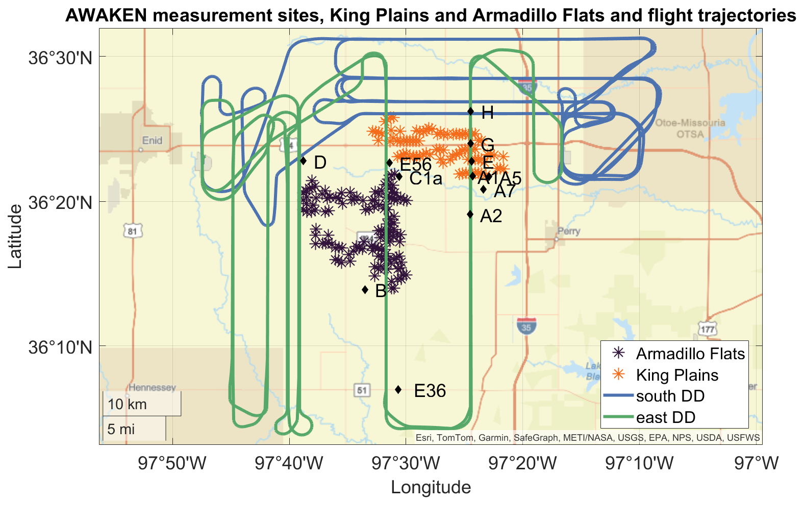
Figure 1 Map of the Armadillo Flats (purple stars) and King Plains (orange stars) wind farms showing the flight trajectories of the research aircraft for Flight 20 for south (blue) and Flight 13 for east (green) wind directions (DD), along with the ground-based measurement sites (black diamonds).

The campaign was conducted in the SGP. This region offers good conditions for field experiments, as the topography is relatively flat and Oklahoma itself is a wind energy hotspot, producing the third-most power from wind energy in the USA in 2022 (Krishnamurthy et al., 2025). The region contains 1000 wind turbines within a radius of 50 km (Letizia et al., 2023), making it interesting for the investigation of cumulative wakes (Debnath et al., 2022; Puccioni et al., 2023). The wind turbines of the wind farms considered in this study are 2.8 MW General Electric (GE) turbines with a hub height of 89 m and a rotor diameter (RD) of 127 m (Debnath et al., 2022; Krishnamurthy et al., 2025; Moriarty et al., 2024). The SGP contains the largest and most extensive climate research site in the world, equipped with several Atmospheric Radiation Measurement (ARM) sites since 1992 (Sisterson et al., 2016). Krishnamurthy et al. (2021) investigated the climatology of the SGP and found that the diurnal cycle of the ABL is particularly pronounced in the summer months. The mean wind speed at 100 m a.g.l. is 7 m s⁻¹, while the mean wind direction is predominantly southeast. These southerly wind directions are typically associated with the formation of nocturnal LLJs. The LLJs occur mainly between 03:00 and 14:00 local time, with the LLJ nose at altitudes below 600 m (Krishnamurthy et al., 2021). The terrain is described as heterogenous, with a gradual west–east slope and distinct diurnal changes in the ABL (Debnath et al., 2022).

2.2 Research aircraft Cessna F406

During the AWAKEN campaign, the research aircraft of Technische Universität (TU) Braunschweig, a Reims-Cessna F406 with the call sign D-ILAB, carried out in situ measurements of temperature, pressure, humidity, wind speed, wind direction, solar and terrestrial radiation, and surface properties. The twin-engine aircraft is well suited to fly at an air speed of 65 to 70 m s⁻¹ and low altitudes of 100 m a.g.l. – close to hub height for offshore applications (Lampert et al., 2024) – allowing high-resolution measurements of atmospheric and surface properties at low altitude. The airflow, temperature, and humidity sensors are mounted on the nose boom in order to sample the undisturbed flow. The three-dimensional wind vector is derived from a five-hole probe in combination with high-precision position and attitude measurements. These measurements are used to calculate the three-dimensional wind vector with a sample rate of 100 Hz, which is used to calculate TKE for 10 s intervals (see Lampert et al., 2024 and Appendix A).

2.3 Flight operations

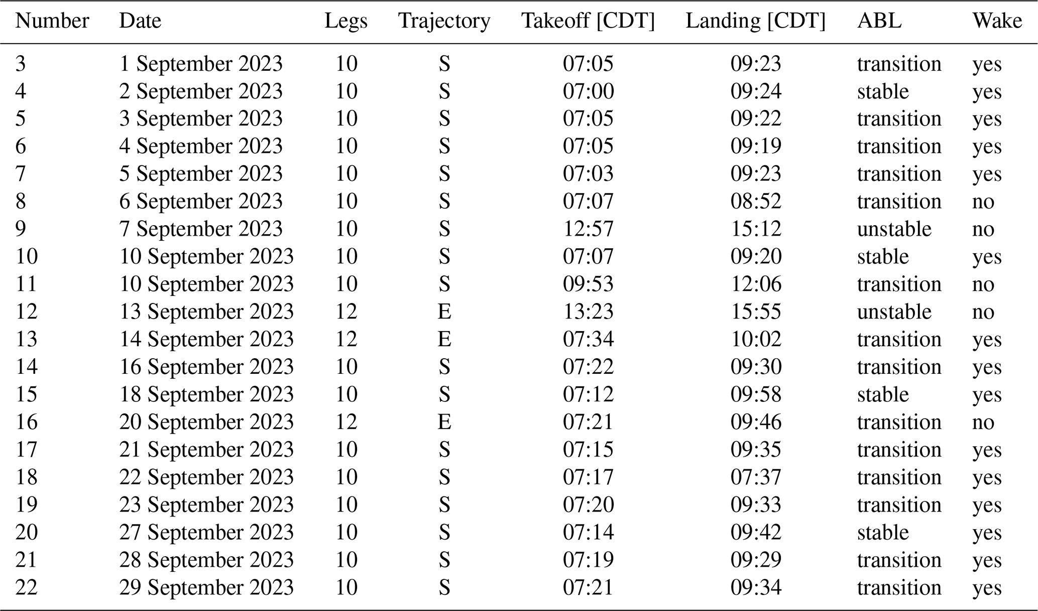
Between 29 August and 29 September 2023, the research aircraft D-ILAB carried out 23 measurement flights over 22 days as part of the project AWAKEN. The research aircraft was stationed at the Enid-Woodring Regional Airport (ICAO identifier KWDG). As the first three flights (Flight 0, 1, 2) were test and adjustment flights, 20 flights are available for analysis. Table 1 provides an overview of the measurement flights, including information on atmospheric stratification and the potential for wake formation. The stratification is estimated based on the vertical potential temperature gradient. The term “transition” refers to cases where the morning transitions were particularly pronounced, resulting in a stably stratified ABL during the initial flight legs and an unstably stratified ABL during later legs (see Table 1, column “ABL”). The last column of the table represents the possibility of the occurrence of a wind farm wake. The days marked “no” indicate that there was no wake formation possible because of an unstable stratification or the predominant wind direction not in the wake segment of 160 to 220° for the King Plains wind farm and 60 to 120° for the Armadillo Flats wind farm.

Table 1 Overview of the flights during the AWAKEN project in Oklahoma by the D-ILAB aircraft, with the number of horizontal legs performed during the flight, southerly (S) or easterly (E) trajectory, flight times, stratification of the ABL (where the transition represents the times when the ABL was stably stratified during the first legs and unstably stratified during the later legs), and whether there were conditions for a wake from either the King Plains or Armadillo Flats wind farms. Flight numbers 1 and 2 were preparation flights and are not included in the analysis.

The trajectories were planned depending on the prevailing wind direction (Fig. 1). As described in Krishnamurthy et al. (2021), the predominant wind direction in this season is south. During the campaign, 17 flights were flown with a predominant southerly wind direction, and three flights were flown with a predominant easterly wind direction. The flights were mostly conducted in the early morning from sunrise at around 07:00 CDT (central daylight time is the local time, corresponding to 12:00 UTC) to 09:30 CDT (14:30 UTC). On most days during the measurement period, due to a strong diurnal cycle of the ABL, a convective boundary layer with strong turbulence formed shortly after sunrise, resulting in an increase in turbulence and a change in stratification from stable to unstable.

To investigate wind farm wakes, horizontal, straight, and level trajectory parts, also referred to as legs, were flown downwind of the wind farms. The trajectory for southerly wind directions, displayed in Fig. 2, consists of vertical profiles and horizontal flight legs. The purpose of the vertical profiles is to examine the ABL to determine the stratification and vertical wind profiles. Several vertical profiles were conducted during each flight at the Perry Municipal Airport (ICAO code KPRO). Figure 2a illustrates the vertical and horizontal profiles including the radar altitude, derived from the equipped radar altimeter and the altitude above mean sea level (a.m.s.l.) plus the digital elevation model (DEM) (U.S. Geological Survey, 2018) derived from the global navigation satellite system (GNSS) and the inertial measurement unit data minus the DEM. These legs cover the width of the wind farm and an extended area to the east of the wind farm in order to compare the wind downwind of the wind farm with the undisturbed flow. The horizontal legs are located at distances of 0.5, 2, 5, and 10 km downwind of the northernmost wind turbine. The northernmost wind turbine was selected as a reference for the distance of the horizontal aircraft legs downwind of the wind farm. This does not reflect the fact that most of the wind turbines are located farther south, resulting in a greater distance from the aircraft measurements to these wind turbines than discussed. Due to Federal Aviation Administration regulations, the research aircraft was not allowed to fly at hub height (89 m); it flew slightly above hub height, varying with the topography between 100 and 160 m a.g.l. (see Fig. 2a). The southerly wind trajectories provide data downwind of the King Plains wind farm (see Fig. 2b).

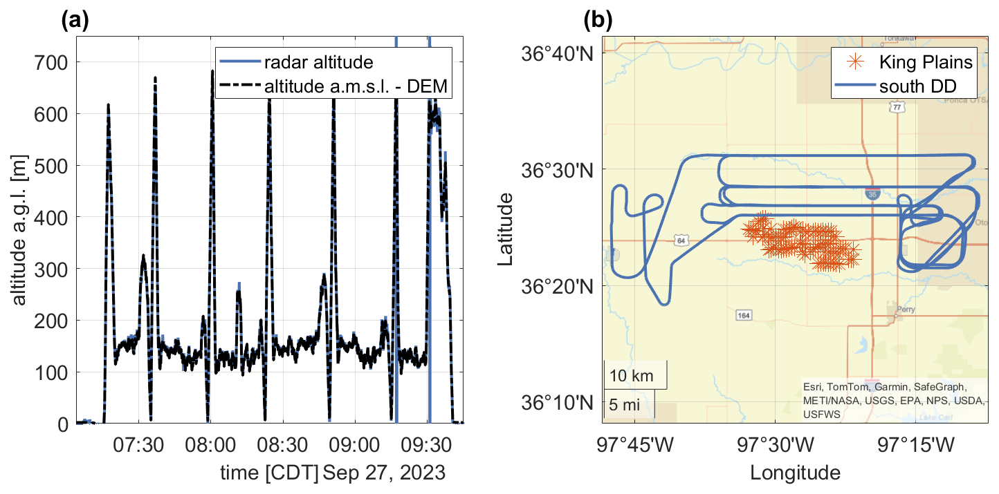
Figure 2 Research flight on 27 September 2023 from 07:14 CDT to 09:42 CDT during southerly wind directions showing the altitude over time (a) and the trajectory on a geographical map including the King Plains wind farm (b).

Due to an unusually high occurrence of easterly wind directions, a second trajectory was flown to investigate the Armadillo Flats wind farm (see Fig. 3). Similar to the southerly wind trajectory, the easterly wind trajectory also consisted of vertical profiles and horizontal legs at varying distances downstream of the last wind turbine. For the easterly wind trajectories, flight legs were performed at distances of 20 and 10 km upwind of the westernmost wind turbine and at distances of 0.5, 2, 4.5, and 9 km downwind of the westernmost wind turbine (see Fig. 3b).

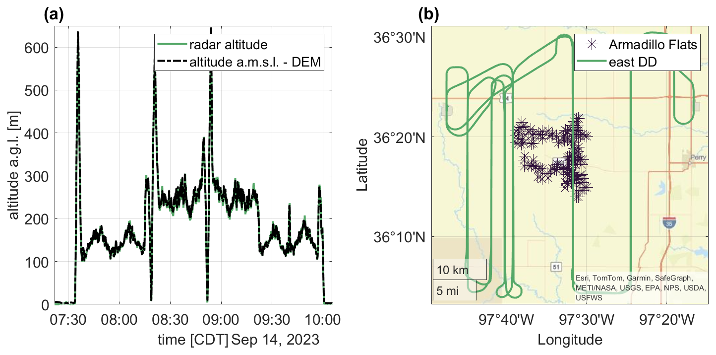
Figure 3 Research flight on 14 September 2023 from 07:34 to 10:02 CDT during easterly wind directions, showing altitude over time (a) and the trajectory on a geographical map including the Armadillo Flats wind farm (b).

2.4 ABL stratification

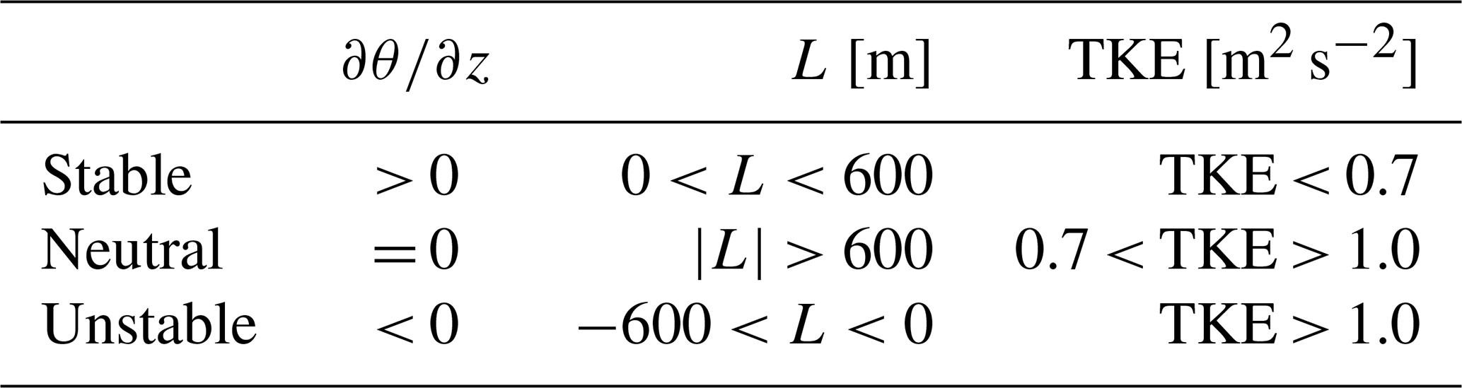
In order to classify the stratification of the ABL, there are three measures used in this study: ground-based TKE measurements from a sonic anemometer, the Obukhov length derived from sonic anemometer data, and the potential temperature derived from vertical profiles of the research aircraft. The Obukhov length and TKE are included in the derived sonic anemometer data (Pekour, 2025). The potential temperature is calculated from temperature and pressure measurements from the research aircraft. For classifying the stratification of the ABL using these measures, this study uses thresholds from Wharton and Lundquist (2012). Table 2 gives an overview of the different stratification classification measures and their thresholds used in this study.

Table 2 Overview of ABL stratification classification measure thresholds for potential temperature gradient $\partial \mathit{\theta }/\partial z$, Obukhov length L, and TKE from Wharton and Lundquist (2012).

3 Results

3.1 ABL stratification during the research flights

Understanding the characteristics of the ABL is crucial for investigating the behavior of wind farm wakes. In this study, most of the measurement flights were conducted shortly after sunrise from 07:00 to 09:30 CDT during the morning transition of the ABL. This has to be considered when interpreting the wake measurements derived from the aircraft data. To get a general idea of the ABL stratification in the SGP region during the measurement flights, data from the sonic anemometer at Site A1 were analyzed. This site was chosen because it is located upwind of the King Plains wind farm and in close proximity to the southernmost wind turbines. To determine the stratification using ground-based measurements, the TKE and the Obukhov length (Monin and Obukhov, 1954) are used. The Obukhov length, calculated near the surface, may not be representative of the rotor layer region of the atmosphere during this time period of rapid evolution (Mahrt and Vickers, 2002; Wharton and Lundquist, 2012). Therefore, a different approach to classifying the stratification using ground-based measurements is the TKE, which is also derived from sonic anemometer data at Site A1. The data are provided with a temporal resolution of 10 min. Figure 4 compares the Obukhov length stratification classification (Fig. 4a) with the TKE stratification classification (Fig. 4b). The classification thresholds are derived from Wharton and Lundquist (2012) (see Table 2). The figures show good agreement between Obukhov length and TKE for the night and midday classifications, with similar frequencies of more than 80 % stable stratification (night) and more than 80 % unstable stratification (midday), while the morning and evening are more smoothly captured by the TKE stratification classification. The theory (Stull, 1988) suggests that the transition is never abrupt and varies daily. Comparing the general occurrences of stratification with the vertical profiles of wind speed and TKE from the lidar at Site A1, the morning transition between sunrise and 09:30 CDT, when most measurement flights were conducted, is clearly characterized. This can be observed, for example, on 10 September 2023 in the lidar data (see Fig. 5). While the wind speed is faster and TKE is weaker between sunset and sunrise, the faster wind speed is lifted upward and the TKE increases from the surface upward after sunrise. When the sun reaches solar noon, the ABL is strongly mixed, characterized by a slower wind speed and a strong vertical signal of TKE. Figure 5a also displays a slight LLJ at the altitudes around 200 m a.g.l., which dissipates after sunrise.

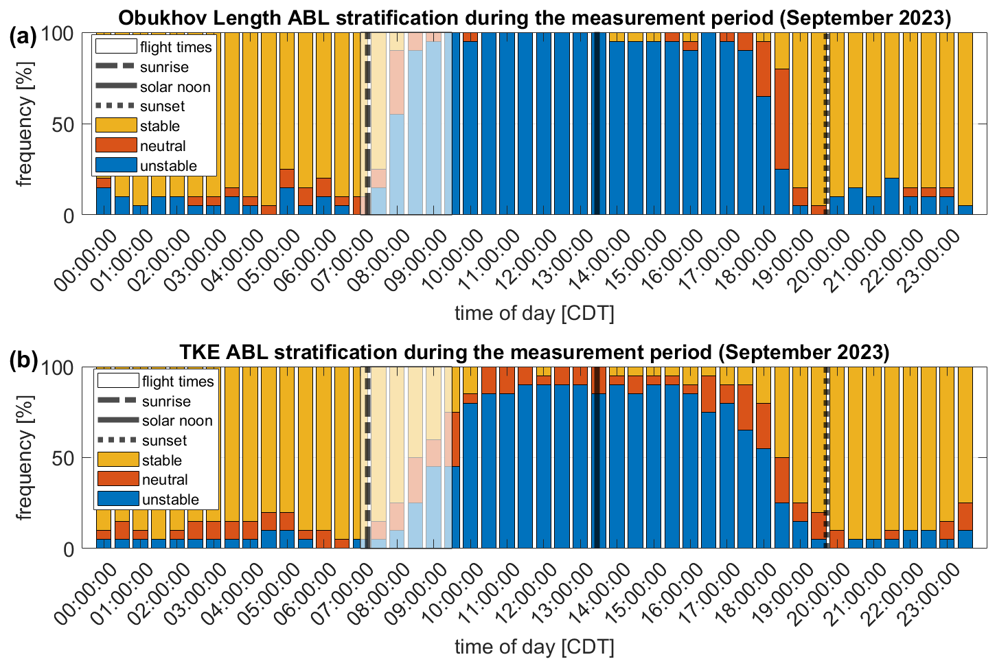
Figure 4 The stratification classification according to Obukhov length (a) obtained by a ground-based sonic anemometer at Site A1 over time of day averaged over the aircraft measurement period (28 August to 29 September 2023) for stable (yellow), neutral (orange), and unstable (blue) ABL stratification, with the mean time of sunrise (dashed-dotted black line), solar noon (black line), and sunset (dotted black line). The approximate aircraft flight times are shown in a white transparent box. Panel (b) shows the stratification classification according to TKE obtained by a ground-based sonic anemometer at Site A1.

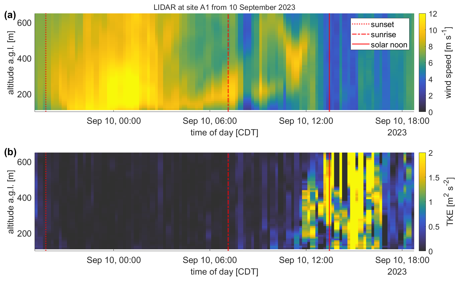
Figure 5 Time series of wind speed (a) and TKE (b) over altitude a.g.l. from 9 September 2023 at 19:00 CDT to 10 September 2023 at 19:00 CDT based on lidar measurements at Site A1, upstream of the King Plains wind farm, with sunset (dotted red line), sunrise (dashed-dotted red line), and solar noon (red line) as an example of the diurnal cycle of the wind speed (a) and the TKE (b) in the SGP region during the aircraft measurement period. Lidar data are available from Bodini et al. (2025).

Aircraft data from this day are displayed in Fig. 6, showing the vertical profiles of wind speed (green) and potential temperature (black) of Flights 10 and 11 from 10 September 2023. The times of the vertical profiles range from 07:07 to 11:44 CDT, with sunrise at 07:12 CDT. The vertical profiles, as part of the flight trajectories, were conducted at Perry Municipal Airport and are therefore in the undisturbed flow and not affected by wind farm wakes.

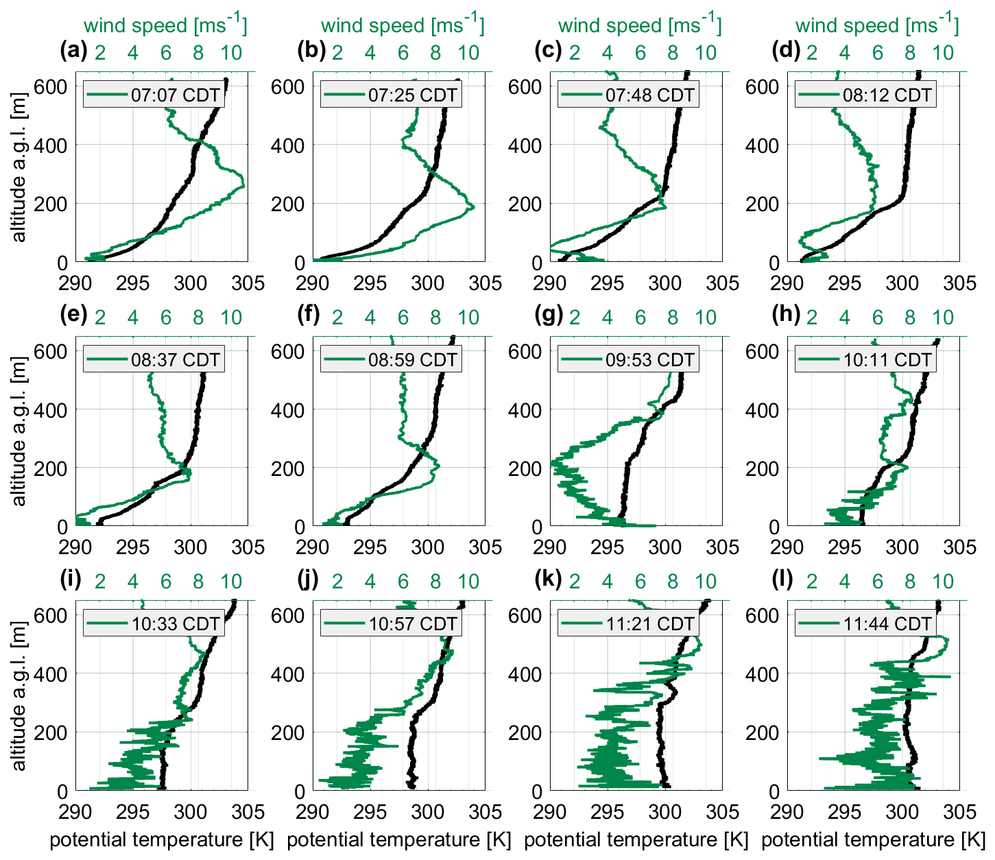
Figure 6 Evolution of the vertical profiles of wind speed (green) and potential temperature (black) recorded by the research aircraft on 10 September 2023 from 07:07 to 11:44 CDT in the undisturbed flow only, showing the ascent.

Characteristic of the stable stratification, a pronounced temperature inversion was observed in the morning between 07:07 and 08:59 CDT, indicated by an increasing potential temperature with height (Fig. 6a–f). From 09:53 CDT on, an unstable layer forms from the ground upward, characterized by a constant potential temperature with altitude and an increase in turbulence. During the course of the morning, the unstable layer continued to grow upward and the turbulence increased in altitude.

In addition to the strong diurnal cycle, this example also shows a superimposed LLJ with a maximum wind speed exceeding 10 m s⁻¹, varying at an altitude of around 200 m a.g.l. The intensity of the LLJ decreased during the morning and dissipated in parallel with the inversion layer at 09:53 CDT. A strong diurnal cycle and an LLJ, dissolving during the morning transition, were also observed during several other measurement flights. Further investigations of the LLJ and the diurnal cycle during AWAKEN were made in Puccioni et al. (2023), Abraham et al. (2024), Krishnamurthy et al. (2025), and Radünz et al. (2025).

3.2 Wind farm wakes in the ABL

The effect of the ABL stratification on offshore and onshore wind farm wakes has been described in several articles (Platis et al., 2018; Lundquist et al., 2019; Cañadillas et al., 2020; Radünz et al., 2021). Whereas Sect. 3.1 illustrated the morning transition of the SGP region on 10 September 2023, this section relates this knowledge to wind farm wakes. First, lidar data from Site A1 (upwind of the King Plains wind farm for southerly flows) and the lidar data from Site H (downwind of the King Plains wind farm for southerly flows) are analyzed. While lidar data are generally a valuable tool for analyzing wind farm wakes, at this measurement site the lidar data lack vertical resolution, with the lowest value occurring at 110 m a.g.l., which is above hub height. The lidar data from Site A1 (see Fig. 7a) display an LLJ at around 200 m a.g.l., which dissipated after 10:05 CDT. This corresponds to the results from the aircraft data displayed in Sect. 3.1. While the lidar data from Site H (see Fig. 7b) also display an LLJ, the LLJ nose is slightly elevated compared to the LLJ at Site A1. A similar phenomenon is described in Krishnamurthy et al. (2025), where the lifting of an LLJ due to the wind farm's internal boundary layer is described. In this study, this phenomenon will not be discussed further, as this study focuses on wind farm wakes. Figure 7c compares the lidar data at Sites A1 and H by displaying the velocity deficit of the wind speed. In order to focus on the wind farm wake, only the velocity below 200 m a.g.l. is considered. A velocity deficit above 50 % at 110 m a.g.l. at 09:05 CDT was detected. The velocity deficit is elevated from 07:35 CDT and decreases after 10:05 CDT. In connection with the vertical profiles obtained by the aircraft (see Sect. 3.1), this can be linked to a transition from a stable to an unstable boundary layer with increasing turbulence. The diurnal cycle – in this case, the morning transition – influences the wind and the behavior of the wind farm wake.

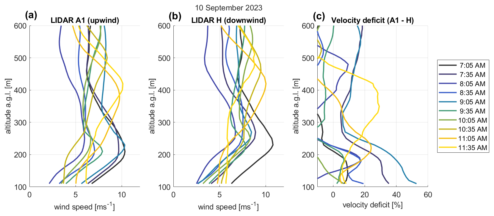
Figure 7 Vertical profiles of wind speed and the impact of wind farm wakes for Site A1 upstream of the wake area (a) and in the wake area (b), and the velocity deficit between the sites (c) on 10 September 2023 between 07:05 and 11:45 CDT (data available through Letizia and Bodini (2024); Bodini et al. (2025), last access: 5 November 2024).

When examining the horizontal legs of the flights, this trend becomes even more pronounced. Figure 8 displays the first four legs of Flight 4 within the time period between 07:08 and 07:49 CDT. This flight is characterized by a stable stratification of the ABL and a distinct wake visible in the wind speed. It is one of two measurement flights where a clear wake could be identified from the wind speed. During the remaining flights, either the wind direction was not adequate for wake analysis or turbulence, and changes in the ABL stratification made the clear identification of the wind farm wake more challenging. In this case, when comparing the area downwind of the wind farm (blue-shaded area) to the free flow, the wind speed downwind of the wind farm is reduced. This suggests that the wake is not fully recovered up to a distance of 10 km from the wind farm (see Fig. 8d). This finding is further supported by the TKE: as the wind turbine blades induce the turbulence, turbulence levels downwind of the wind farm increase compared to the free flow. With increasing distance from the wind farm, the turbulence downwind recovers but remains more pronounced than in the free flow (Fig. 8e–h). In addition, Fig. 8e illustrates a significant peak in TKE at the west end of the King Plains wind farm. This structure is also visible in the wind speed measurements, displayed as gray dots (see Fig. 8a) and is likely linked to the layout of the wind farm. The turbines at the west end are located closer to the horizontal flight legs compared to the wind turbines at the east end (see Fig. 2b). The TKE peak can also be associated with higher wind shear at the edge of the wind farm, as observed for offshore wind farms in Cañadillas et al. (2023). This suggests that to identify and understand the wake, TKE can be a helpful tool in addition to the wind speed.

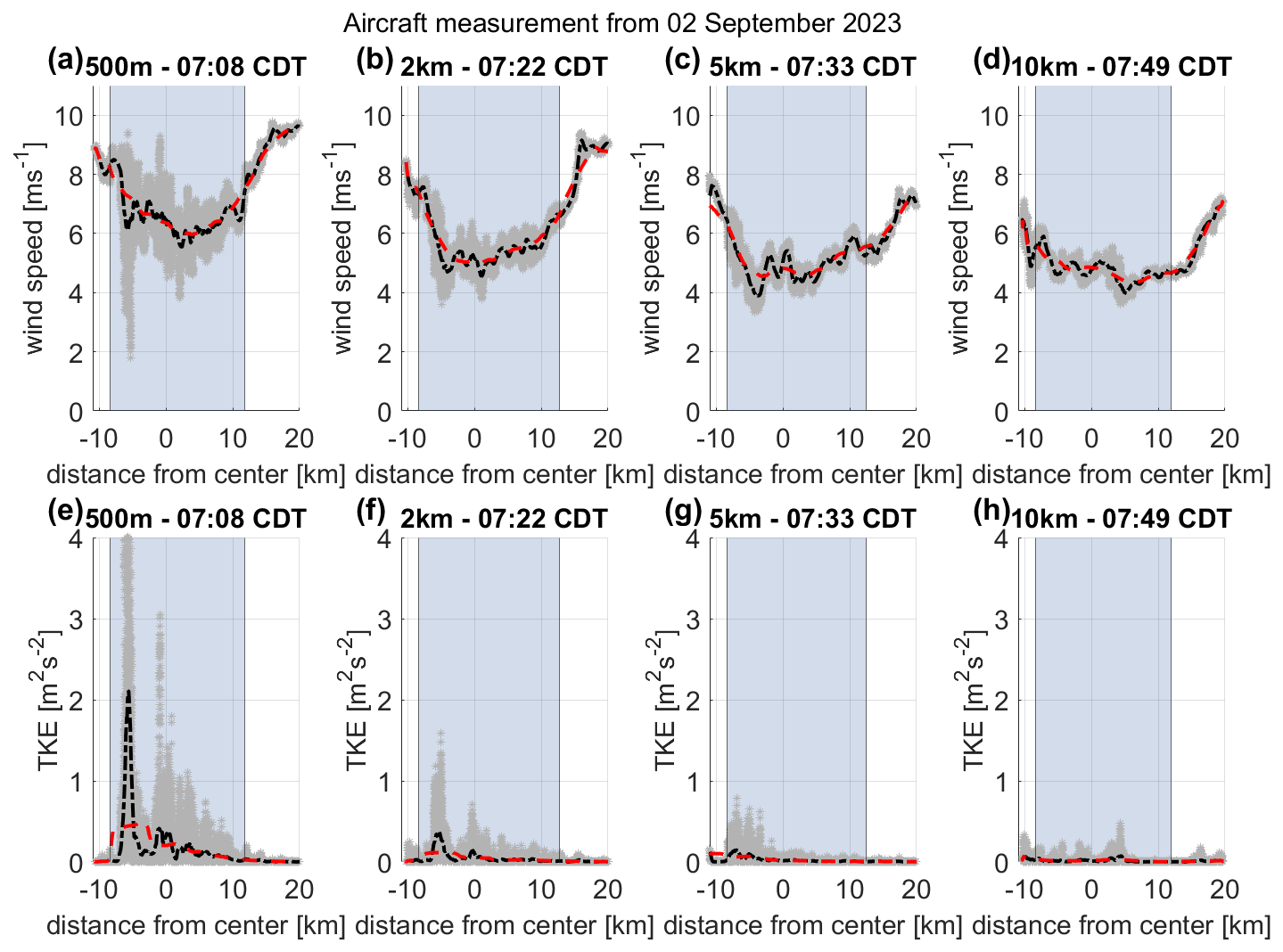
Figure 8 Illustration of wind speed and TKE (gray dots), median average over 0.78 km (dashed-dotted black line), and median average over 6.07 km (dashed red line) for first four legs of Flight 4 with respect to the distance from the center of the King Plains wind farm (blue-shaded area).

To get a general idea of the different wake behavior in TKE and in wind speed, Fig. 9 combines data for all legs of the research flights with the occurrence of a wake in the morning at the King Plains wind farm. This includes all flights marked with “yes” in the wake column of Table 1 with a southerly trajectory (“S”). For each leg at the corresponding distance downwind of the wind farm (0.5, 2, 5, 10 km), the median wind speed and TKE were calculated for 200 m segments. This overview shows that the TKE downwind of the wind farm is increased compared to the free flow; this is pronounced at a distance of 10 km downwind of the wind farm (Fig. 9h). On the other hand, the wind speed downwind of the wind farm shows a different behavior. There is no clear structure in the wake compared to the free flow. In this general overview, the wake changes width and deficit compared to the natural variability in the free flow. It is expected that the wind speed in the free flow should be higher compared to the wind speed in the wake for legs closer to the wind farm, which is not the case. This raises the question of whether there are other phenomena influencing the spatial distribution of the wind speed, such as topography or stratification.

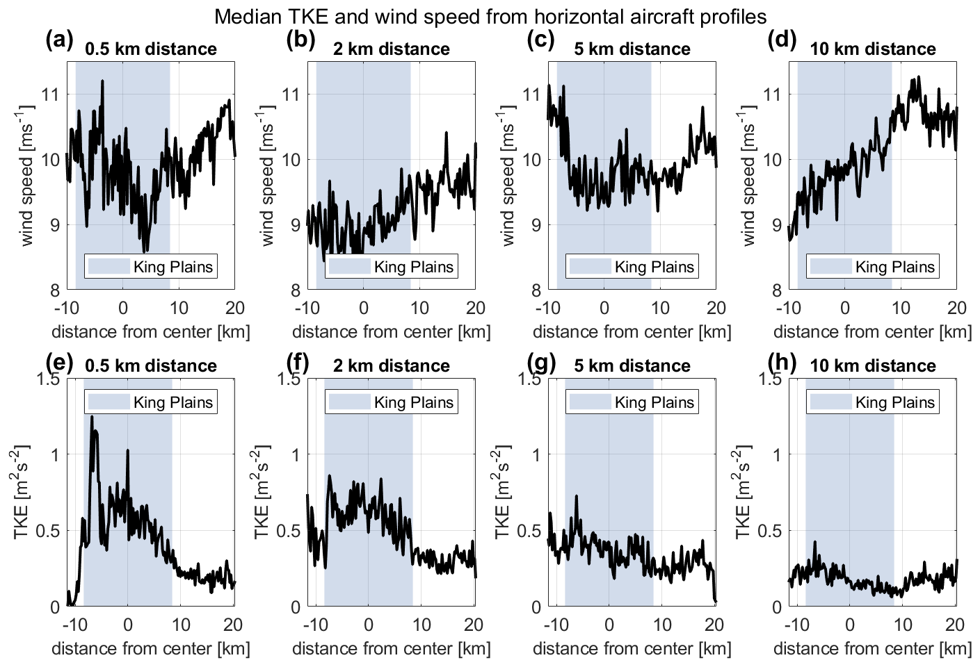
Figure 9 Illustration of median wind speed (a–d) and median TKE (e–h) from all wake measurement flights over a horizontal distance of 200 m from the center of the King Plains wind farm (shaded-blue area) with different distances downwind of the King Plains wind farm (0.5, 2, 5, and 10 km).

To highlight the effect of stratification on wake recovery, Fig. 10 displays the difference in TKE in the wake and in the free flow and the velocity deficit for flights in stable, neutral, and unstable ABL stratification. The stratification was derived from the TKE of a ground-based sonic anemometer at Site A1 (see Sect. 2.1). The statements presented in this section are only based on the flight measurements but are not statistically significant because of limited data availability. Figure 10d–f highlights the trend of a wake recovery, based on the TKE difference, with increasing distance from the wind farm and a strong wake during stable conditions close to the wind farm, a weaker wake close to the wind farm for neutral conditions, and no distinct wake for unstable conditions. Previous studies of offshore wind farms have used the velocity deficit of the wind speed downwind of the wind farm and in the free flow (Krishnamurthy et al., 2017). Figure 10a–c displays the velocity deficit for the same flights and stratification. The limited number of data weakens the conclusions drawn from these data. While the trend for the velocity-deficit-based wake recovery downwind of the wind farm is noisier compared to the TKE difference, the magnitude of the velocity deficit decreases from stable to neutral to unstable conditions. The TKE difference for stable and neutral conditions in 5 km displays higher values compared to the TKE difference in 10 km; this cannot be observed in the velocity deficit for the same conditions. The velocity deficit in 10 km is generally higher than the velocity deficit in 5 km. Because of limited data availability, more measurement flights are needed to investigate the TKE difference in addition to the velocity deficit as an indicator for wind farm wakes and their recovery.

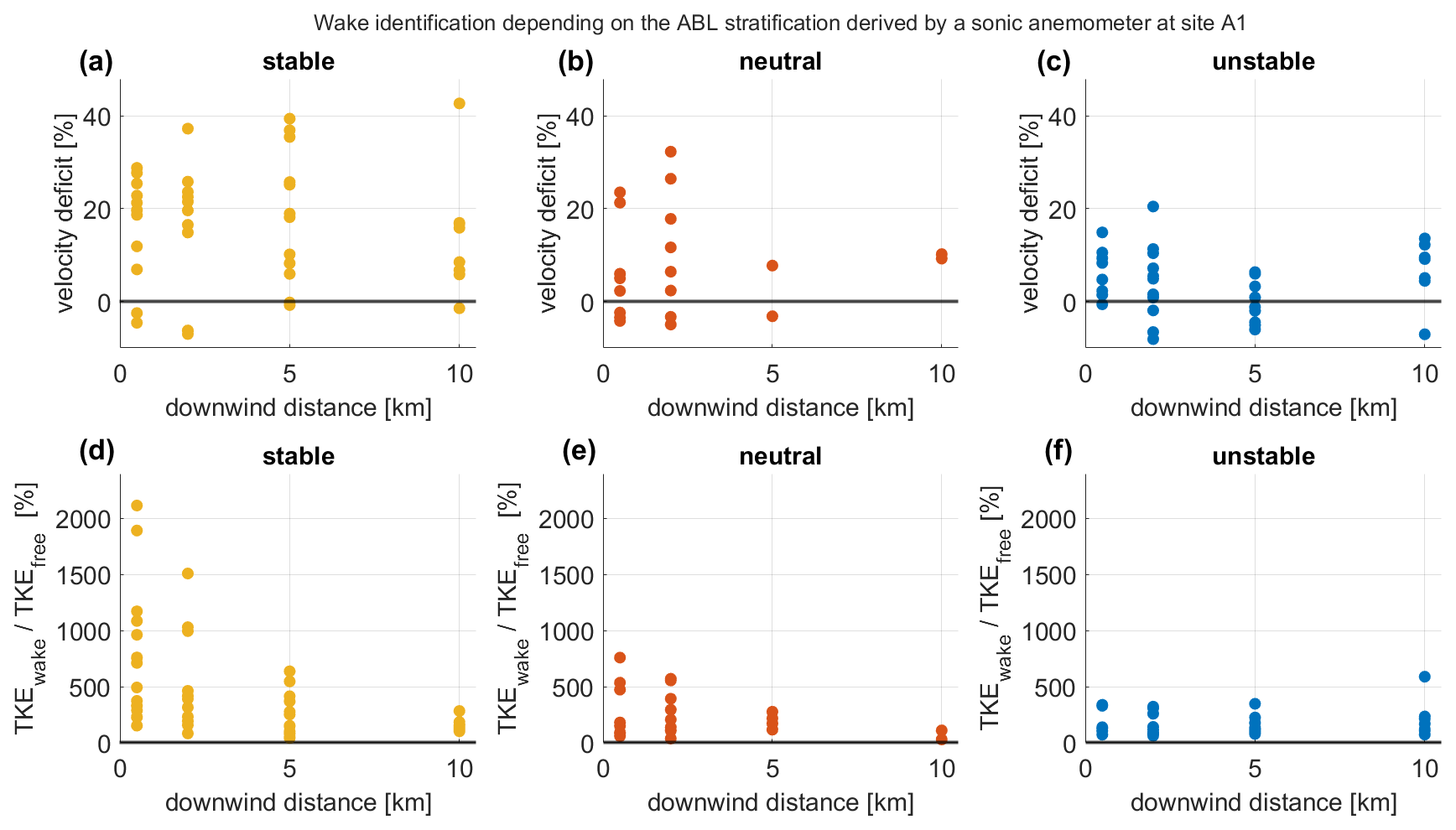
Figure 10 The velocity deficit of the wind speed in the wake compared to the wind speed in the free flow from aircraft measurements for stable (a), neutral (b), and unstable (c) conditions derived from the TKE of the sonic anemometer at Site A1. The median TKE in the wake compared to the median TKE in the free flow (d–f) downwind of the King Plains wind farm.

3.3 Wind farm wakes in semi-complex terrain

When analyzing the data, there are characteristics in the wakes that cannot be explained by only considering the wind speed. For onshore wind farms, in contrast to offshore wind farms, there are the effects of the earth surface influencing the flow patterns and of the ABL stratification. In addition to the strong diurnal cycle in the SGP region, the terrain also slopes eastward. In this study, the terrain is referred to as “semi-complex”, as it is not technically complex but shows differences in elevation of 100 m over a distance of 10 km.

In cases where the wind direction was predominantly easterly (Flights 12, 13, 16), the aircraft flew a different trajectory to survey the Armadillo Flats wind farm. In these cases, the terrain downwind of the wind farm is at a similar altitude as the terrain where the Armadillo Flats wind farm is located. This is supported by the fact that the wind comes from a southeasterly direction. Figure 11 illustrates Flight 12 on 14 September 2023. Figure 11a shows the terrain and the wind farm, the horizontal legs, and the arrows for the corresponding wind direction. This case will be treated as a homogeneous terrain because the wake is located at the same altitude as the wind farms. In Fig. 11b–e, the wake and the free flow at different distances downwind of the wind farm are shown. The first four legs were performed at 07:40 CDT in a stably stratified ABL. The wake recovers at a 9 km distance from the wind farm (Fig. 11b), where the velocity deficit is significantly lower compared to the legs closer to the wind farm. This trend is also visible in Fig. 11f–i for the later flight at 09:22 CDT, where the ABL transitions to an unstable stratification. The velocity deficit is lower than in the earlier legs, and in this case the wake has fully recovered at 9 km downwind of the wind farm, displaying a velocity deficit of −2.77 % (Fig. 11i).

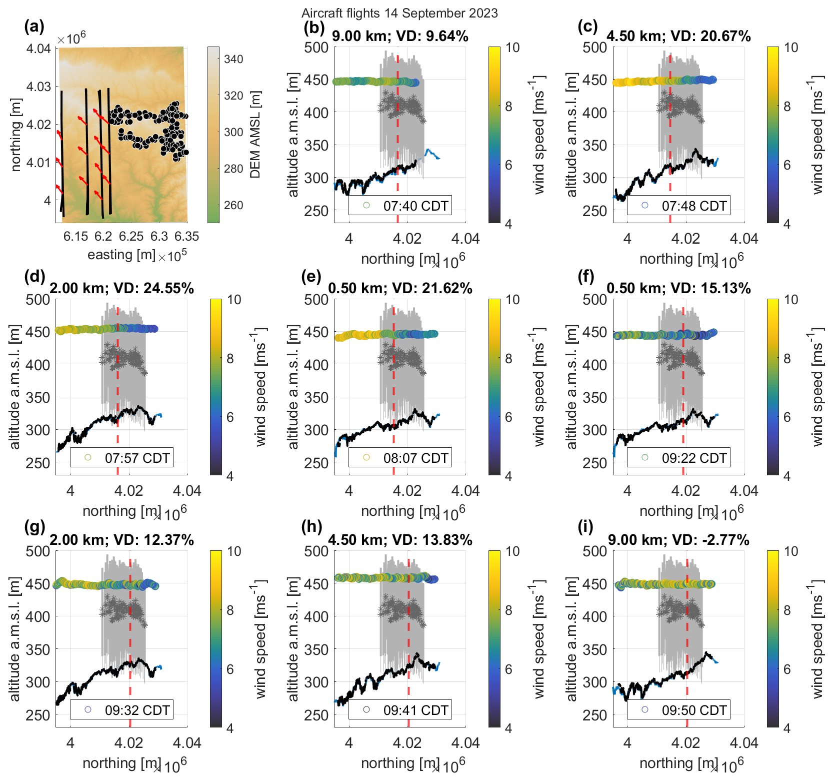
Figure 11 Wake analysis for easterly wind direction. (a) Overview of the legs (parallel black lines), the Armadillo Flats wind farm (black/white dots), and the wind direction across the legs (red arrows). (b–i) The wind turbines of the Armadillo Flats wind farm (gray lines), the hub heights (gray stars), the topography obtained from the digital elevation model (blue line, U.S. Geological Survey, 2018), and the cut-off line (dashed red line) between the wake and the undisturbed area to calculate the velocity deficit (VD), derived from lidar data at Site A1 for the time of the leg at 110 m a.g.l. The wind speed is color coded.

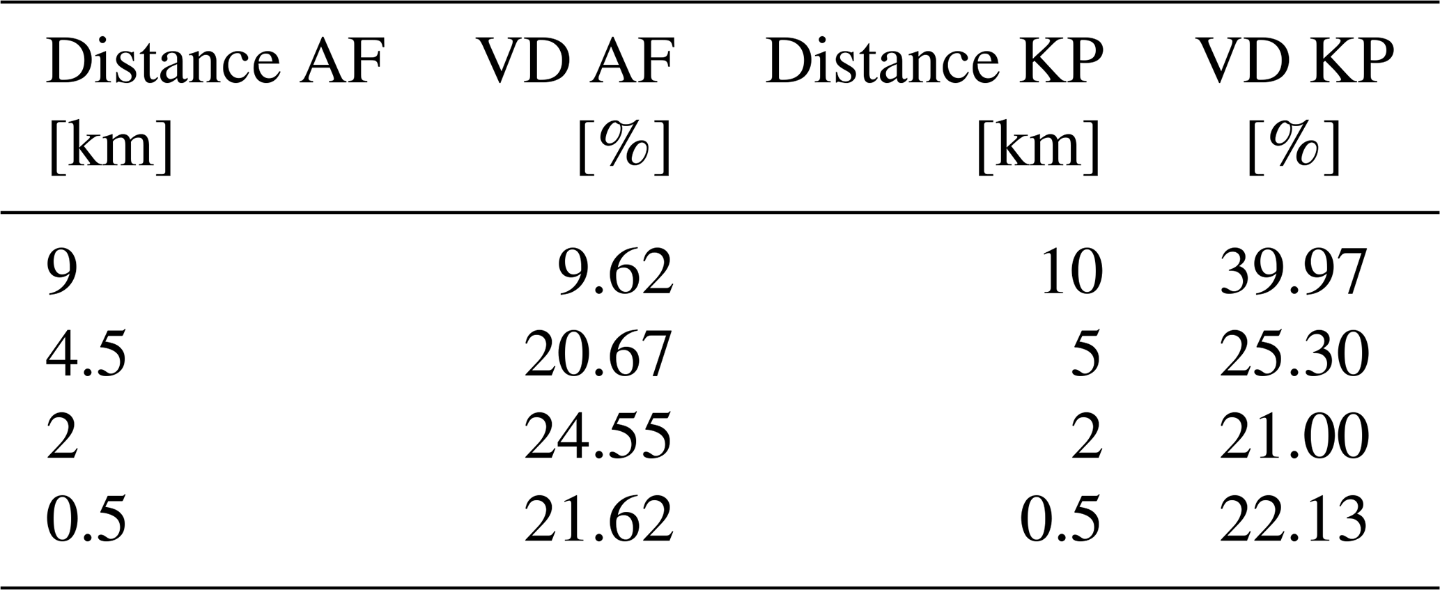
In contrast to the homogeneous terrain, the terrain downwind of the King Plains wind farm is characterized by a slight hill on which the wind turbines are located, a valley at 260 m a.m.s.l. at approximately 5 km downwind of the wind farm, and an upward slope at 320 m a.m.s.l. at 10 km distance downwind of the wind farm (see Fig. 12a). As described in Stull (1988) and Kaimal and Finnigan (1994), hills alter the flow by accelerating and decelerating it. Depending on the stratification of the ABL, the flow downwind of the hill will follow the terrain in stable conditions or will be lifted by buoyancy in unstable conditions. Figure 12b–k displays the wind speed at different distances downwind of the wind farm. The wind speed displays clear wakes in all distances downwind of the wind farm. To isolate the potential influence of the terrain on the wind farm wake, Table 3 compares the velocity deficit of the legs in similar distances downwind of the King Plains wind farm (KP, semi-complex terrain) and the Armadillo Flats wind farm (AF, homogeneous terrain). The first leg of the flight in homogeneous terrain was conducted at 07:40 CDT, and the first leg of the flight in complex terrain was conducted at 07:21 CDT. The velocity deficit in 0.5 and 2 km is of similar magnitude to the homogeneous and complex terrain. While in the homogeneous terrain, the velocity deficit decreases at a distance of 4.5 km and it increases at a distance of 5 km in the complex terrain. This trend strengthens as the velocity deficit in the homogeneous terrain decreases further at a distance of 9 km from the wind farm, whereas it increases even further in the complex terrain case. In both cases, the wind farm wake is not fully recovered at these distances, as the threshold for recovery is < 5 %. For these two flights, the aircraft data might be able to detect an effect of the terrain on the wind farm wake, displaying an amplification of the velocity deficit with increasing distance in the semi-complex terrain.

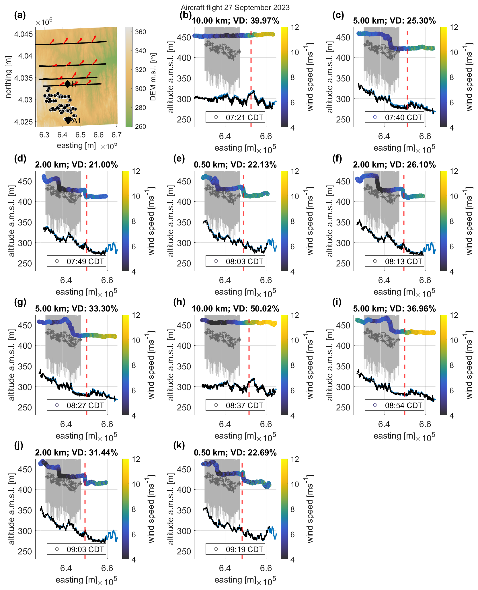
Figure 12 Wake investigation for southerly wind direction. (a) Overview of the legs (parallel black lines), the King Plains wind farm (black/white dots), and the wind direction across the legs (red arrows); (b–i) the wind turbines of the King Plains wind farm (gray lines), the hub heights (gray stars), the topography obtained from the digital elevation model (blue line, U.S. Geological Survey (2018)), and the cut-off line (dashed red line) between the wake and the undisturbed area to calculate the velocity deficit (VD), derived from lidar data at Site A1 for the time of the leg at 110 m a.g.l. The wind speed is color coded.

Table 3 Overview of the velocity deficit (VD) values and the corresponding distances from the Armadillo Flats (AF, homogeneous terrain) and King Plains (KP, semi-complex terrain) wind farms.

4 Discussion

Wind farm wakes are mainly investigated using ground-based measurement systems, with certain limitations concerning the spatial resolution and span of the measurements. Aircraft measurements provide an addition to ground-based measurement systems, as they have a higher spatial resolution and are able to capture wakes at different distances downwind of the wind farm. In this study, wind farm wakes at 10 km downwind of the wind farm were detected. Although the aircraft measurements are an important tool for learning more about wind farm wake behavior, there are also limitations. First, the flight legs flown downwind of the wind farm are not performed simultaneously. As shown in the vertical profiles of potential temperature, there is a strong diurnal cycle in the ABL in the SGP, and therefore the wake behavior changed from the beginning to the end of each flight. Second, the influence of the ABL on the wind farm wakes was strong; therefore, measurement flights during the middle of the day were not useful for wake detection when there was strong convection. This can be observed for some measurement flights that started during sunrise, with the last legs indicating a convective boundary layer. For the investigation of the stratification of the ABL in addition to vertical profiles of potential temperature measured by the aircraft, the TKE from ground-based measurement sites proved to be a reliable parameter compared to the Obukhov length. The comparison of the ABL stratification and the wakes was similar to what has already been investigated for offshore wind farms. In addition, in this study of onshore wind farm wakes, a strong influence of the topography on the wake was observed, and some cases even show an amplification of the wake effect at 5 to 10 km downwind of the King Plains wind farm. The database of the measurement flights is not sufficient to derive statistically significant conclusions, but an effect from the terrain is visible when comparing the wake and the flow pattern downwind of the King Plains and Armadillo Flats wind farms. This raised the question of whether the TKE could be a better indicator of the wind farm wake than the wind speed. The wind speed obtained by the aircraft is measured at a resolution of 100 Hz and is therefore sensitive to gusts and other atmospheric anomalies. The turbulence representative, TKE, was derived from the variance of 100 Hz wind components filtered with a 0.1 Hz cut-off, representing the energy of turbulent fluctuations over about 10 s (approximately 650 m along-track distance). This approach reduces the influence of the natural background wind variability and provides a statistically robust measure of turbulence and hence wind farm wakes. When analyzing the TKE difference between the wind farm wake and the free flow, the TKE increases downwind of the wind farm and in stable conditions, displaying a near-logarithmic decay of the TKE deficit with increasing distance from the wind farm. In contrast, the commonly used velocity deficit struggles to represent clear wind farm wakes with the highest velocity deficits of over 50 % at 10 km downwind of the King Plains wind farm in stable ABL conditions. The wind speed is the most interesting value to the wind farm operators, as it determines the optimal distance between the wind farms to ensure high inflow speeds. In this case, the TKE seems to provide a better understanding of the wind farm wake width and length.

5 Conclusions

This study demonstrated that there are similar effects when comparing onshore and offshore wind farm wakes, for example, the dependency on ABL stratification. However, there are many factors that need to be considered for onshore wind farms that can be neglected for offshore wind farms, for example, a strong diurnal cycle and the topography, including the surface roughness and albedo. During the measurement period, the SGP region showed a strong diurnal cycle of the ABL, with multiple occurrences of LLJ events. For the stratification classification, TKE data from a ground-based sonic anemometer were used according to Wharton and Lundquist (2012). This supports a further understanding of the wind farm wakes in a quickly changing ABL. Even though aircraft measurements were conducted approximately 20–50 m above hub height, the wakes were distinguishable in the horizontal aircraft legs and the lidar data at Site H. The combined lidar and aircraft data showed the vertical and horizontal extent of the wind farm wakes. This study investigated the effect of the topography using aircraft data and was able to show that specific topographic features such as valleys and hills may lead to an amplification of the wind farm wake. This effect was most pronounced in the wind speed, while the analysis of the TKE in the wake and the free flow better indicated the actual length of the wake. As a conclusion, TKE might not be the most important parameter for the wind industry, but it can give an idea of the persistence of wakes in complex conditions. Nevertheless, this study supports the fact that wind farm owners may need to consider topography, which may amplify wakes, and reduce wind speed for wind farms farther downwind under certain conditions. Future work might include a thorough comparison of onshore and offshore wind farm observations and a weather research forecasting model comparison to further understand the wind field in semi-complex topography.

Appendix A: Wind measurements on board D-ILAB

The basic principle for determining the wind vector v_w on board the D-ILAB aircraft is to calculate the difference between the ground speed vector v_g and the air speed vector v_a.

$$\begin{array}{}\text{(A1)}& {\mathit{v}}_{\mathrm{w}}={\mathit{v}}_{\mathrm{g}}-{\mathit{v}}_{\mathrm{a}}\end{array}$$

The ground speed vector v_g = $\left(v_{\mathrm{North}},v_{\mathrm{East}},v_{\mathrm{Down}}\right)$ is directly output by the iNAT-RQT-4001 inertial navigation system (INS; iMAR, Germany) and is the result of a tightly coupled INS/GNSS-based data fusion using 42+ state Kalman filtering. The iNAT-RQT-4001 is further described in Lampert et al. (2024). The integrated GNSS receiver OEM6 (NovAtel, Canada) is capable of L1L2 GPS+GLONASS+GALILEO+BEIDOU as well as SBAS. Internally, accelerations and angular rates are measured at a rate of 400 Hz, but only 100 Hz data from the integrated INS/GNSS solution are available for position, velocity, and attitude angles. The basis for determining the air velocity vector in the geodetic coordinate system is Lenschow's system of equations (Lenschow, 1972). Air velocity (true air speed, or TAS), angle of attack (α), and angle of sideslip β) are determined by measuring total air temperature (TAT) (Rosemount 102DB1AG, USA), static pressure P_stat, dynamic pressure P_dyn, and the differential pressures of dPα and dPβ using a five-hole probe (Rosemont 858, USA) and corresponding pressure sensors (Setra, USA) at a sampling rate of 100 Hz. Great attention is paid to the correction of probe errors, installation errors, and temperature errors, as well as the lever arm corrections by positioning the sensors in the measuring head of the nose boom instead of the aircraft's center of gravity. For a coordinate transformation from the aircraft fixed to the geodetic coordinate system, attitude angles (Φ, Θ, Ψ) are also required, which in turn are taken from the inertial navigation system to calculate the air velocity vector v_a = $(u,v,w)$ in the geodetic coordinate system v_ag = $(u_{\mathrm{g}},v_{\mathrm{g}},w_{\mathrm{g}})$.

$$\begin{array}{}\text{(A2)}& {\displaystyle }\begin{array}{rl}{u}_{\mathrm{g}}=\text{TAS}(& \cos \mathit{\alpha }\cdot \cos \mathit{\beta }\cdot \cos \mathrm{\Theta }\cdot \cos \mathrm{\Psi }\\ & +\sin \mathit{\beta }\left(\sin \mathrm{\Phi }\cdot \sin \mathrm{\Theta }\cdot \cos \mathrm{\Psi }-\cos \mathrm{\Phi }\cdot \sin \mathrm{\Psi }\right)+\end{array}\text{(A3)}& {\displaystyle }\sin \mathit{\alpha }\cdot \cos \mathit{\beta }\left(\cos \mathrm{\Phi }\cdot \sin \mathrm{\Theta }\cdot \cos \mathrm{\Psi }+\sin \mathrm{\Phi }\cdot \sin \mathrm{\Psi }\right))\text{(A4)}& {\displaystyle }\begin{array}{rl}{v}_{\mathrm{g}}=\text{TAS}(& \cos \mathit{\alpha }\cdot \cos \mathit{\beta }\cdot \cos \mathrm{\Theta }\cdot \sin \mathrm{\Psi }\\ & +\sin \mathit{\beta }\left(\sin \mathrm{\Phi }\cdot \sin \mathrm{\Theta }\cdot \sin \mathrm{\Psi }+\cos \mathrm{\Phi }\cdot \cos \mathrm{\Psi }\right)\end{array}\text{(A5)}& {\displaystyle }\sin \mathit{\alpha }\cdot \cos \mathit{\beta }\left(\cos \mathrm{\Phi }\cdot \sin \mathrm{\Theta }\cdot \sin \mathrm{\Psi }-\sin \mathrm{\Phi }\cdot \cos \mathrm{\Psi }\right))\text{(A6)}& {\displaystyle }\begin{array}{rl}{w}_{\mathrm{g}}=\text{TAS}(& -\cos \mathit{\alpha }\cdot \cos \mathit{\beta }\cdot \sin \mathrm{\Theta }+\sin \mathit{\beta }\cdot \sin \mathrm{\Phi }\cdot \cos \mathrm{\Theta }\\ & +\sin \mathit{\alpha }\cdot \cos \mathit{\beta }\cdot \cos \mathrm{\Phi }\cdot \cos \mathrm{\Theta })\end{array}\end{array}$$

Thus, the wind components in the meteorological sense are calculated as follows:

$$\begin{array}{}\text{(A7)}& {\displaystyle }{u}_{\mathrm{wg}}=v_{\mathrm{East}}-v_{\mathrm{g}}\text{(A8)}& {\displaystyle }{v}_{\mathrm{wg}}=v_{\mathrm{North}}-u_{\mathrm{g}}\text{(A9)}& {\displaystyle }{w}_{\mathrm{wg}}=-v_{\mathrm{Down}}+w_{\mathrm{g}}.\end{array}$$

A bottleneck for the accuracy of wind measurement is the pressure measurement. Thermal effects, hysteresis, and non-linearities also negatively influence the measurement accuracy. Due to the comparability of the measurement technology of the former research aircraft D-IBUF, the accuracy of the horizontal wind speed component should be specified as < 0.5 m s⁻¹, as described in Corsmeier et al. (2001), and that of the vertical wind speed component as < 0.1 m s⁻¹. Calibration and comparison flights with both research aircraft were carried out and confirm this assumption. A detailed description of the aircraft's instrumentation is given in Lampert et al. (2024).