Exploring future production scenarios for Italian offshore wind power

This study explores the potential of offshore wind energy in Italy by considering the planned offshore wind farms, their construction challenges, possible wake losses, and production based on historical data (by using ERA5 and CERRA dataset). An IEA 15 MW wind turbine was considered for all locations, since the turbine models have not yet been decided in the preliminary plans. A genetic algorithm was used to identify a tentative optimal layout able to maximize the minimum intra-turbine distance without considering the local wind rose, obtaining an estimate of wake losses for each planned farm. By means of Monte Carlo simulations, future energy scenarios are assessed, considering factors such as technical challenges, wind patterns, turbine characteristics, and array efficiency due to wake effects, offering valuable insights into the feasibility of the planned offshore wind energy in Italy or in other countries with similar wind resources.

1 Introduction

Human activities, particularly those associated with the burning of fossil fuels and industrial processes, have led to a significant increase in greenhouse gas emissions. These emissions are the primary drivers of global climate change, posing substantial challenges to environmental sustainability and human wellbeing. To address these challenges, renewable energy (and wind energy in particular) stands out as a promising solution in the transition towards low-carbon energy sources. Wind energy is nowadays an established technology with several key players worldwide. Since the wind resource is higher offshore due to the lower surface friction, offshore wind energy has been an interesting alternative to onshore installations due to a higher social acceptance (Walker et al., 2014). However, offshore installations have a higher cost due to development challenges and infrastructure, connection, foundation construction, and maintenance costs. They have therefore been limited to areas with sea depth up to 50 m (Rodrigues et al., 2015) and high wind resource, such as northern European waters. Floating turbines provide the opportunity to perform offshore installations in other locations characterized by much higher sea depth, opening new scenarios for offshore installations (Wang et al., 2010).

Italy, with its extensive coastline and favorable wind conditions, has a significant potential for offshore wind energy development. While offshore wind technology has been extensively deployed in regions like the North Sea, Italy's unique geographic and environmental characteristics present both challenges and opportunities for offshore wind projects. The development of offshore wind projects in Italy, which aims to support 3.8 GW of wind power by 2028 through a contract for a difference scheme recently approved by the European Commission (the FER2 Decree, https://www.mase.gov.it/portale/-/energia-mase-pubblicato-il-decreto-fer2, last access: 23 February 2026), requires a holistic approach, encompassing wind patterns, correlations between different Mediterranean zones, and future energy production scenarios. It is acknowledged that the recent round of bidding in the summer of 2025 has not included offshore projects. Nevertheless, the Italian Government has set ambitious targets for 2030 in the recently submitted Integrated National Energy and Climate Plan (PNIEC) document to the European Union. That is, renewables should contribute to almost 40 % of the gross energy consumption. Developers have shown a significant interest in the opportunities of the Italian offshore market, leading to 84 GW of connection requests to the grid owner TERNA at the end of September 2024 (TERNA, 2024). The current study aims to address these aspects by analyzing historical wind data, developing statistical models, and simulating future energy scenarios using Monte Carlo techniques. Through data-driven analysis and modeling, our objective is to provide valuable insights into the potential of offshore wind energy deployment in Italy.

Correlation analysis can provide valuable information on the decision-making process regarding the construction of wind farms, ensuring that energy production does not overwhelm the grid infrastructure (Vladislavleva et al., 2013). Correlation analysis and production assessments between various zones can predict instances of excessive energy production, posing challenges to the electrical grid, market balance, and potentially storage development. In general, the correlation of wind power output between wind farms decreases with distance and varies with timescales and wind patterns, suggesting the prioritization of interconnection between zones with low correlation to optimize wind power production and smooth variability. Many studies (Olauson and Bergkvist, 2016; Malvaldi et al., 2017; Ren et al., 2020) have analyzed the correlation between wind farms using actual wind power production data and their related separation distances, leading to an exponential decrease in the correlation with the increase in distance. Real-time data from one area can help forecast wind power in another by considering their correlation and time lag. This approach leads to a more stable and predictable power system, reducing costs, emissions, and energy consumption (Malvaldi et al., 2017). Therefore, it is essential to explore the available Italian projects and their distribution to gain a comprehensive understanding of the situation and estimate the expected power production. This study delves into the main aspects of wind farm projects and aims to provide a probabilistic approach to a possible production scenario.

The paper is organized as follows: Sect. 2 provides background on the wind resource in the Mediterranean Sea near Italy from both the ERA5 and CERRA databases and the existing farm projects and associated grid connections. An analysis of the unlagged and lagged correlation coefficients is shown in Sect. 3 together with an assessment of the capacity factor due to only wind availability. Given the different challenges of each project, a multi-criteria analysis is discussed in Sect. 4, leading to the definition of a score value indicating the challenge class or the construction probability. The simplified layout definition and the associated wake losses of each farm are evaluated in Sect. 5, followed by Sect. 6, which presents the results of the Monte Carlo simulations. Finally, Sect. 7 concludes the paper with a summary of key findings and implications for offshore wind energy development in Italy.

2 Site description

A total of 55 different offshore Italian wind farm projects are selected among those presented to the Ministero dell'Ambiente e della Sicurezza Energetica (MASE), distributed over the Italian shore, and clustered in about 35 geographical areas (https://map.tgs4c.com/offshorewind/, last access: 23 February 2026) (hereafter referred to as “clusters” to highlight that the wind features of each cluster are common for all farms embedded into it). From the MASE website, it was possible to obtain key information about the planned installed capacity, such as the number and type of turbines of the farm projects, the coordinates of the wind farm areas under development, the distance from the shore, and the indicative grid connection option. Figure 1 shows the considered projects where each farm is marked by its respective bounding polygon. It is possible to see that some wind farms are very close to each other, and some even overlap: due to their proximity, it is considered that two neighboring farms experience the same wind speed regime; therefore only the centroids of the farm clusters are considered in the wind speed analysis. The centroid was calculated as the arithmetic mean of the latitude and longitude of the bounding polygon. Given the centroid (latitude–longitude), the velocity time series at the nearest grid points were downloaded from the CERRA database and linearly interpolated to the centroid location.

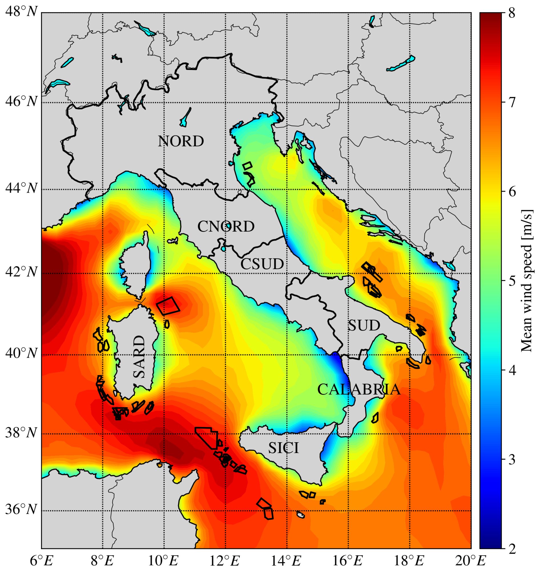
Figure 1 Average wind speed magnitude around the Italian shore from the ERA5 dataset (Hersbach et al., 2020) at a height of 100 m a.s.l. The seven TERNA zones are also marked on the map. The planned wind farms are marked by black polygons.

For the overlapping projects, the shared area is considered to be equally split between the two wind farms, assuming that the developers will reach an agreement to bring both projects forward. The capacity of each farm is then calculated by subtracting half of the overlapped percentage capacity as

$$\begin{array}{}\text{(1)}& \begin{array}{rl}\text{new capacity}& =\text{initial capacity}\\ & \times \left(\mathrm{1}-{\displaystyle \frac{\mathrm{1}}{\mathrm{2}}}\times \text{overlapped percentage}\right).\end{array}\end{array}$$

Since the projects are distributed all around the country, it is possible to distinguish between different geographical zones. In particular, the Italian National Electricity Grid (named TERNA) divides the Italian territory into seven zones, as highlighted in Fig. 1. These zones allow operators to trade efficiently and avoid network security issues. TERNA reorganization of the electrical market zones aims to provide accurate price signals, prevent speculation, and accurately reflect market conditions. Each of the 55 wind farm projects can be associated with one of these zones depending on the indicative grid connection. The seven zones are North Italy (NORD), Central North Italy (CNORD), Central South Italy (CSUD), South Italy (SUD), Calabria (CALABRIA), Sicily (SICI), and Sardinia (SARD).

The mean wind speed is highest for the farms around Sardinia and near Sicily, while it is lower in the northeast. To give an idea of the wind energy potential and its variability, Fig. 2 shows the 90th percentile of wind speed magnitude, highlighting again that the projects near Sicily and Sardinia are characterized by a significant wind resource, more significant than for the Puglia and Romagna regions.

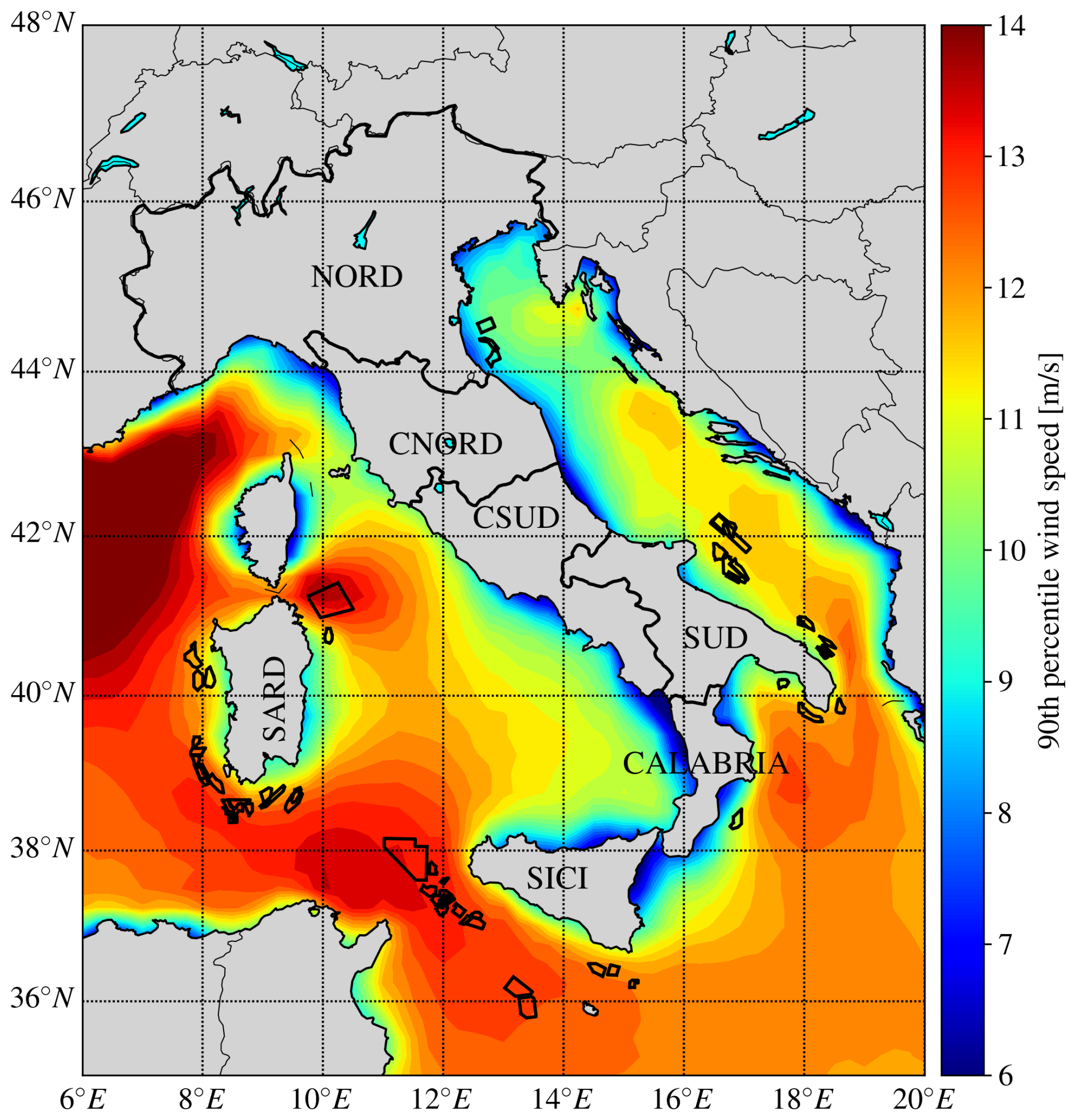
Figure 2 90th percentile of wind speed magnitude around the Italian shore from the ERA5 dataset (Hersbach et al., 2020) at a height of 100 m a.s.l. The planned wind farms are marked by black polygons.

The wind speed at each area, or wind farms cluster, is key to understanding the climatology of different sites in the Mediterranean Sea. This study used the wind speed time series obtained from 35 different areas around the Mediterranean Sea over 31 years (from 1 January 1990 to 31 December 2021) at 100 m a.s.l. to obtain a comprehensive time history of the site representative of the cluster climate. The data were obtained from the Copernicus European Regional Reanalysis (CERRA, Schimanke et al., 2021), which is a regional reanalysis dataset developed and optimized for the entire European area, including sea areas with a horizontal resolution of 5.5 km and a temporal resolution of 3 h covering 37 years from 1984 to 2021. The CERRA system uses ERA5 global reanalysis (Hersbach et al., 2020) as lateral boundary conditions, and data assimilation is used to improve the accuracy of the numerical solver (Kalnay, 2003). Alternative datasets could have been chosen for this task, such as the ERA5 or the NEWA databases (Hahmann et al., 2020; Dörenkämper et al., 2020). However, ERA5 was not used due to the poorer spatial resolution (of the order of 27 km), while NEWA was not selected since no data assimilation was adopted in the wind atlas generation (except for the ERA5 data used at the simulation boundaries). Nevertheless, it is noted that the correlation between ERA5 and CERRA was very high across all 35 clusters with correlation coefficients around 92 % (the lowest correlation was 83 % for one of the farms in the NORD TERNA zone). The analysis of the correlations between different clusters, presented later in the paper, is also qualitatively similar between the CERRA and the EMD WRF Europe+ (EMD, 2024) datasets. In the NEWA dataset, the WRF mesoscale model is run in an optimized configuration at a high spatial resolution of 3 km to produce hourly time series based on ERA5 reanalysis data from European Centre for Medium-Range Weather Forecasts (ECMWF) as a boundary condition. In conclusion, and given the available datasets, the wind speed values at each specific cluster were determined through a linear interpolation process for both the ERA5 and CERRA datasets, although only the latter will be used in the power analysis of the various farms also considering its free access and benefit to the wider research community.

The bathymetric value of the Mediterranean seabed was also assessed as an important parameter in the farm construction. For each of the 55 considered projects, the average sea depth was estimated by means of the General Bathymetric Chart of the Oceans (GEBCO; Weatherall et al., 2015) database (2022 release). The database provides gridded elevation data in meters, combining satellite altimetry predictions with observational data. Figure 3 shows the sea depth around the Italian coast and provides an assessment of the sea depth for each wind farm. 18 % of the planned farms are located at a sea depth of less than 100 m, while 24 % are planned at a sea depth of 500 m or more, and the remaining 58 % of the planned farms are located at a sea depth between 100 m and 500 m.

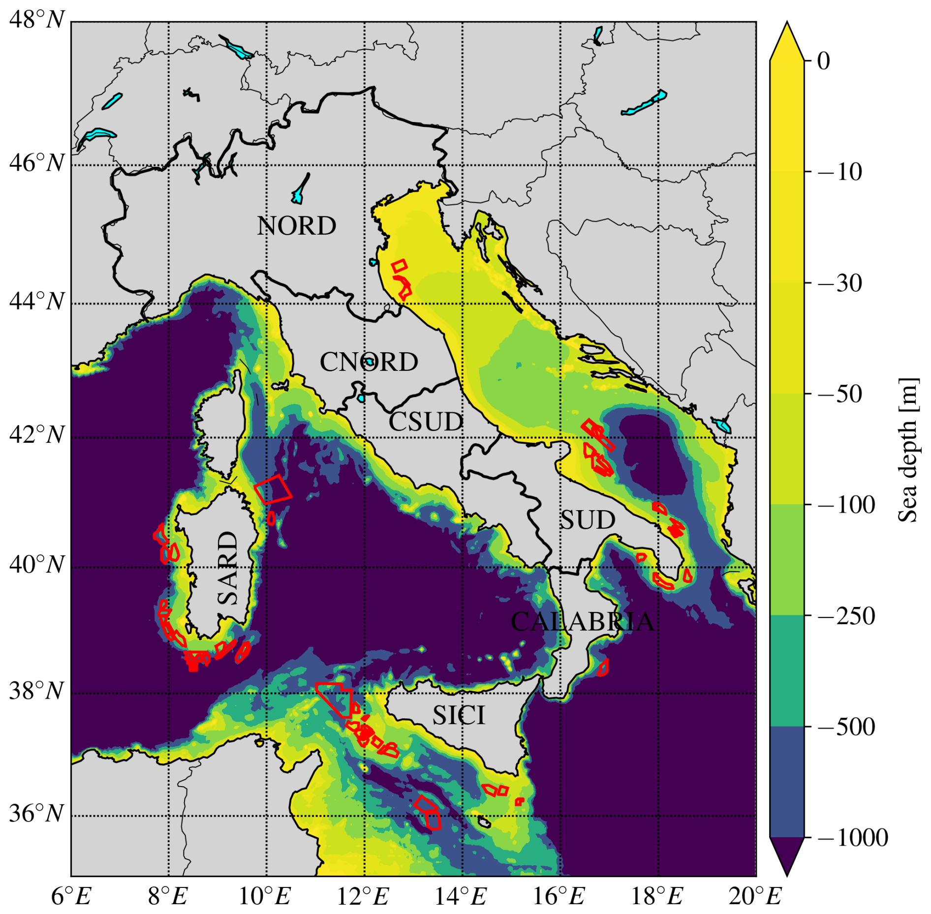
Figure 3 Bathymetry of the Mediterranean Sea near Italy from the GEBCO dataset (Weatherall et al., 2015). The planned wind farms are marked by red polygons.

Finally, since many sites did not provide a precise turbine model, the IEA 15 MW turbine model (Gaertner et al., 2020) was used for all projects. This turbine was chosen since it is internationally recognized and used in other studies (Gaertner et al., 2020; Papi and Bianchini, 2022) and since it is considered representative of a high-quality turbine model. The number of turbines selected for each wind farm was determined from the ratio between the planned installed capacity of the farm and the turbine rated power output (15 MW). The turbine has a cut-in speed of 3 m s⁻¹ and a cut-out speed of 25 m s⁻¹, and it should therefore encompass the majority of the wind conditions experienced in the Mediterranean Sea. The rotor diameter is 240 m, while the hub height is 150 m. Since wind speed data are available at a height of 100 m a.s.l. but the IEA 15 MW turbine hub height is 150 m, a correction to the historical time series is applied by using a power-law wind profile with a shear exponent of 0.1, close to the suggested value from the IEC 61400 norm and within the variability of the shear exponent in offshore conditions (Dhomé et al., 2025): this implies that the wind speed time series at each cluster will be multiplied by a factor of $(\mathrm{150}/\mathrm{100}{)}^{\mathrm{0.1}}=\mathrm{1.041}$. The power curve of the turbine is shown in Fig. 4. This turbine was chosen regardless of the foundation characteristics, i.e. by assuming that even floating turbines should have similar dimensions and performance.

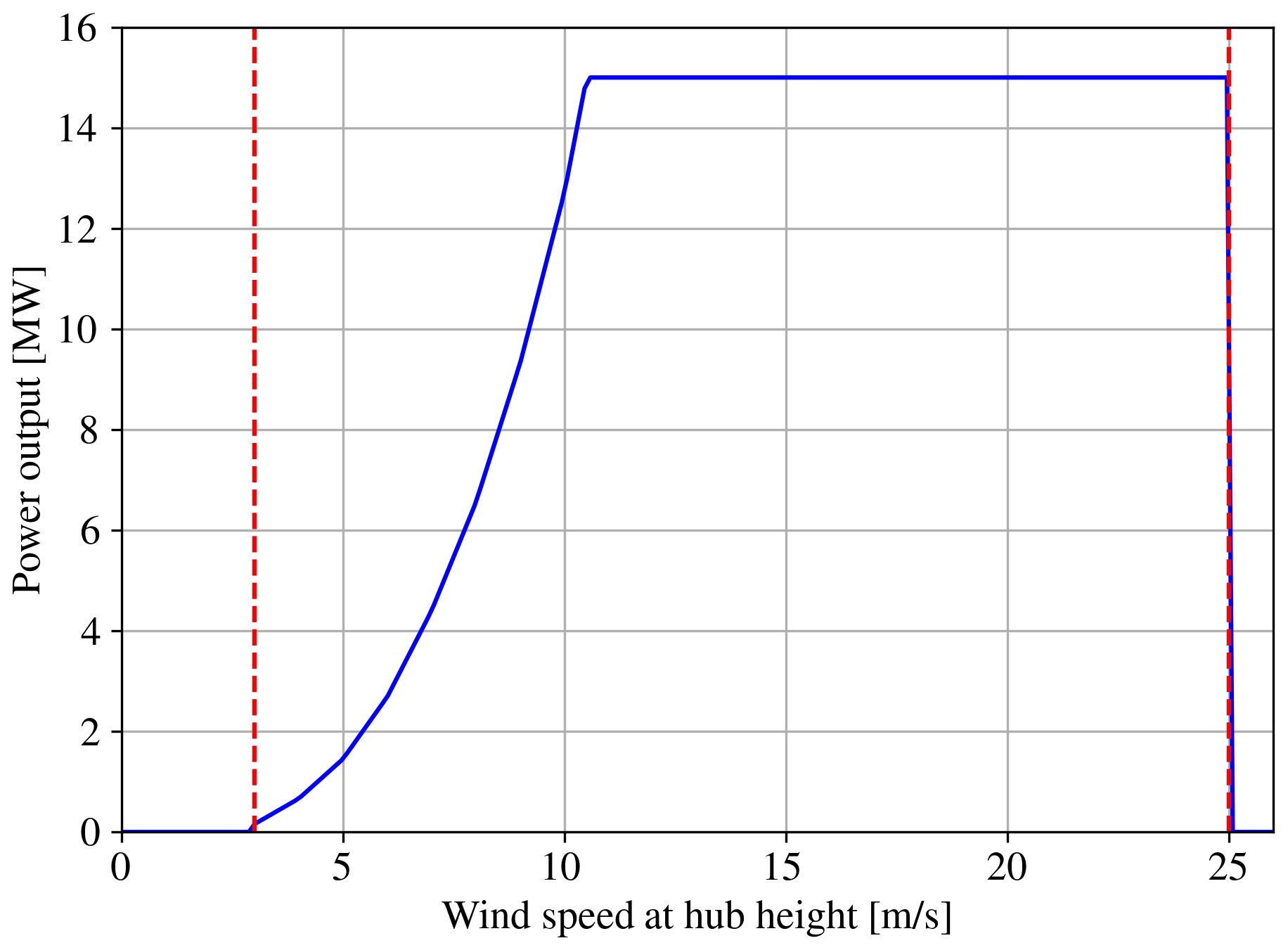
Figure 4 Power curve of the IEA 15 MW turbine. The characteristic wind speeds of cut-in and cut-out are marked with red dashes.

3 Correlation analysis and capacity factors

A goal of this project is to explore the presence of meaningful correlations in wind speed patterns across various zones of the Mediterranean Sea. Understanding the correlation within a certain time lag range is essential for assessing the synchronization of wind patterns between two wind farms, optimizing energy production strategies. Specifically, the aim is to discern whether the selected 35 clusters, designated for future wind farm projects, exhibit significant spatial correlations in terms of both wind speed and power. Figure 5 shows the Pearson correlation coefficient between the power production associated with a single IEA 15 MW turbine located in one cluster and the power production of another IEA 15 MW turbine in another cluster. No wake losses or additional transmission losses are accounted for in the correlation analysis shown in Fig. 5. The power signals are obtained from the historical wind speed time series at the various clusters converted into power by means of the IEA 15 MW turbine power curve. The correlation could also be done in terms of velocity magnitude only (bypassing the need for a power curve), but the results are qualitatively similar.

Figure 5 Power correlation coefficient between different clusters.

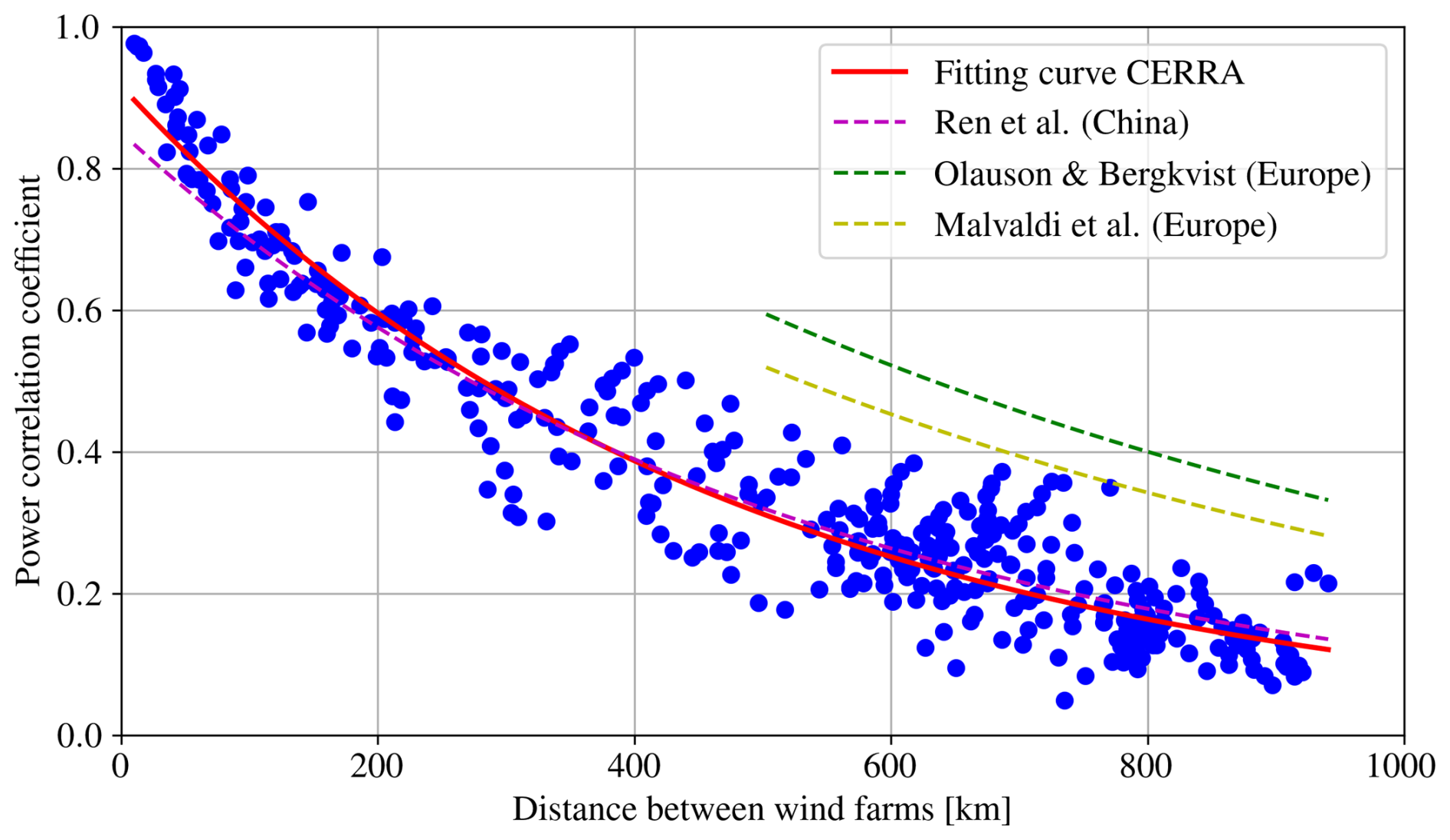
Figure 5 shows the expected result that farms located nearby experience highly correlated power production (within 100 km the correlation is generally higher than 80 %), while the correlation drops to less than 20 % for farms located more than 500 km apart. A power law of the form $\mathit{\rho }=A\exp (-\mathrm{\Delta }/B)$ was fitted to the data points, where ρ and Δ indicate the Pearson correlation coefficient and the distance between farms, respectively. The fitting constants are identified as A=0.919 and B=471.8 km. The exponential law does not properly describe the farms separated by short distances, but it fits the data reasonably well otherwise, considering the scatter due to different geographical characteristics. It is interesting to note that the obtained power law is in agreement with the power law obtained in China by Ren et al. (2020), but it is below the correlations reported by Olauson and Bergkvist (2016) and Malvaldi et al. (2017), mostly because these last two correlations focused mainly on wind farms located in the North Sea, where the wind resource is higher and the wind farms might operate more often at rated conditions. Furthermore, the latter studies are characterized by larger distances between the projects, so that the fittings are weighted more towards large-distance farms, explaining the larger B value reported in the above-mentioned studies. A similar behavior is observed for the correlations in the North Sea by Hjelmeland and Nøland (2023), whose paper includes a variation of the coefficient by the averaging period as well. The reason behind the similarity between our correlations and the Chinese correlation of Ren et al. (2020) might be due to similar wind characteristics between China and Italy, since they both have lower wind intensity compared to northern Europe.

By introducing a time lag between the power production, it is possible to investigate whether the correlation might be higher with some time shift. The analysis is complicated by the fact that the wind direction, the wind magnitude, and the distance between farms should influence the time shift associated with the highest correlation between two wind farm clusters, although this dependency was not taken into account in the present analysis. Results of a lagged correlation analysis are shown in Fig. 6 for three wind farms located in Puglia (SUD zone), Sicily (SICI zone), and Sardinia (SARD zone), sufficiently far apart to make the analysis worthwhile.

Figure 6 Lagged power correlation coefficient between three different farms.

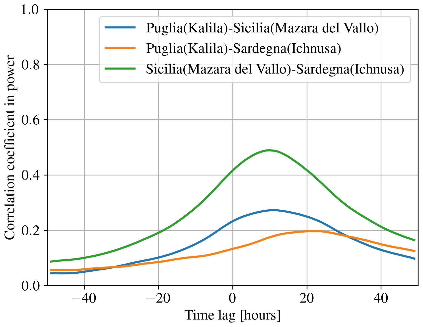
It can be seen that an optimal time lag of around 10–20 h exists between the farms, although the maximum correlation coefficient is of the same order as the correlation coefficient with zero time lag. Once again, the optimal time lag depends on the chosen farm pair and the dominant wind speed and direction, and it is anyhow expected to depend on the wind properties at both sites. Similarly, there are also opportunities with projects which are clearly uncorrelated, as demonstrated by the challenges for the North Sea offshore grid (Hjelmeland and Nøland, 2023), where it was shown by the authors how a decreased correlation was leading to a lower variability of the energy production from a portfolio of wind farms.

Given the complexity of identifying a correlation model, the historical time series were considered over more than 30 years to be sufficiently representative of the wind speed climatology at the various clusters, already embedding the correlations between various farm locations. This consideration will guide the Monte Carlo simulations described in Sect. 4.

The next aspect to be considered is the capacity factor of all the clusters, which is the ratio between the long-term average power production of an isolated wind turbine located at the cluster centroid and its rated power. By assuming for simplicity a Weibull distribution and the power curve to be a cubic power law of the velocity before rated speed and flat afterwards, it is possible to show that the capacity factor depends primarily on the average wind speed (and weakly on the shape factor of the Weibull distribution). Figure 7 shows the power ratio for all the considered clusters, demonstrating that even for the IEA 15 MW power curve and for realistic wind occurrence frequencies (which may or may not be Weibull-distributed), the capacity factor grows linearly with the mean wind speed with a slope of 0.089 s m⁻¹.

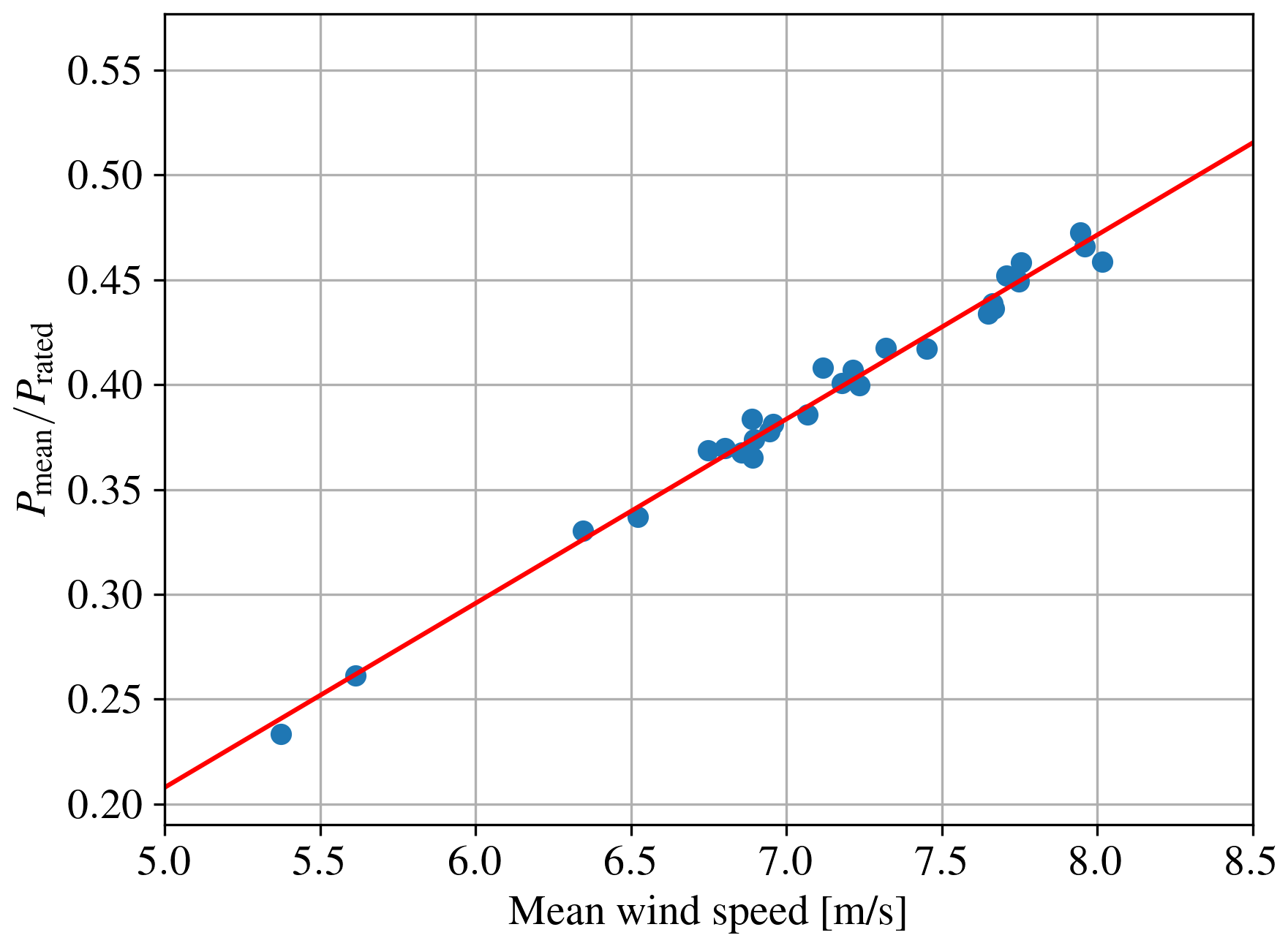
Figure 7 Blue circles: ratio between the average power of an isolated turbine and its rated power for different mean wind speed. Red line: $P_{\mathrm{mean}}/P_{\mathrm{rated}}=\mathrm{0.089}{U}_{\mathrm{mean}}-\mathrm{0.241}$ (with U_mean in m s⁻¹).

All the planned single wind turbines have a capacity factor of less than 50 %, clustering around 40 % with two outliers down to 20 %–25 %. The reader is reminded that Fig. 7 is associated with wind availability and is not affected by other losses such as wake losses, meandering (Medici and Alfredsson, 2006), blockage (Segalini and Dahlberg, 2020), and transmission losses.

4 Challenge analysis and Monte Carlo simulations

Since the 55 selected wind farm projects are still in the development phase, it can be expected that some will not pass the initial stage. The construction challenge of each project is assessed by considering factors such as wind patterns, distance from the shore, seabed conditions (its depth in particular), and wind farm characteristics to identify the best areas for offshore wind deployment. We have arbitrarily identified four technical parameters which will pose a certain level of challenge for each project, namely (i) the mean wind speed, (ii) the installed capacity, (iii) the water depth, and (iv) the distance from the shore. The decision to employ the mean wind speed is driven by the aim to estimate long-term energy production rather than to verify resilience to extreme conditions. In contrast, the water depth and the distance from the shore will necessarily pose challenges in terms of floaters, anchors, and dynamic cables.

For the detailed calculation, a score value is assigned to each variable from 1 to 3 based on the predefined ranges shown in Table 1, although it is acknowledged that some level of uncertainty should be expected with such an arbitrary choice.

Table 1 Scoring system of the influencing parameters.

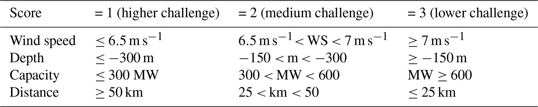
The individual scores were then combined to calculate a total score as

$$\begin{array}{}\text{(2)}& \text{total score}={\displaystyle \frac{\mathrm{1}}{\mathrm{4}}}\left(\sqrt{\sum _{i=\mathrm{1}}^{\mathrm{4}}{x}_i^{\mathrm{2}}}-\mathrm{2}\right),\end{array}$$

where x_i is between 1 and 3 and is the score for the ith variable. The total score is normalized to be a number between 0 and 1, where 0 means very high challenge and 1 means low challenge or higher probability that the project will overcome the four technical parameters combined. Other parameters could be considered. Seabed characteristics are a possible complexity in the construction and hence an additional challenge to the development; however, these are the result of detailed geophysical investigations. Although in principle it is possible to review the reports included in the environmental authorization procedure, only a few projects have completed these studies. Beside the obvious time-consuming effort, the task would bias the scoring system. The advancement into the permitting process, the complexity of the grid connection works, and the access to measured data might also be considered. The electrical connection is a parameter to be ideally included: however, we have decided to focus on the production rather than on the LCOE of each project. The parameter is partly (and implicitly) included in the distance to the shore. We believe that other factors related to the electrical design, unknown at this stage, can play a significant role: number of offshore substations, inter-array cable design, point of connection at the TERNA substation onshore, to cite a few. It is believed that the initial set of parameters can be further implemented; however, there is a risk associated with over-complexity as well. The scoring system is based on the same weight for all selected parameters, but it is reasonable to expect that increasing the number of parameters will necessarily require the introduction of a weighting matrix to evaluate the risk against the effect on the development. Nevertheless, to implement a transparent approach, a risk matrix requires detailed information which is not yet considered available at this stage of the development of the offshore market in Italy for most of the 55 projects considered. This is especially true since we aim at comparing the projects relatively to each other and not in an absolute way. We therefore consider that the added uncertainties of a risk matrix might introduce a bias in the results.

The results of the evaluation are illustrated in Fig. 8. For the sake of simplicity, now and in the following, farms belonging to the TERNA zones NORD, CNORD, CSUD, and CALABRIA are accounted for together. Projects with a score below 0.5 are considered to face higher challenges in addressing the four parameters than those with a challenge level exceeding 0.6–0.7. The most resourceful wind farms are located in Sicily and Puglia. Many projects in Sardinia are instead facing higher challenges due to the high sea depth and the need for larger floating installations.

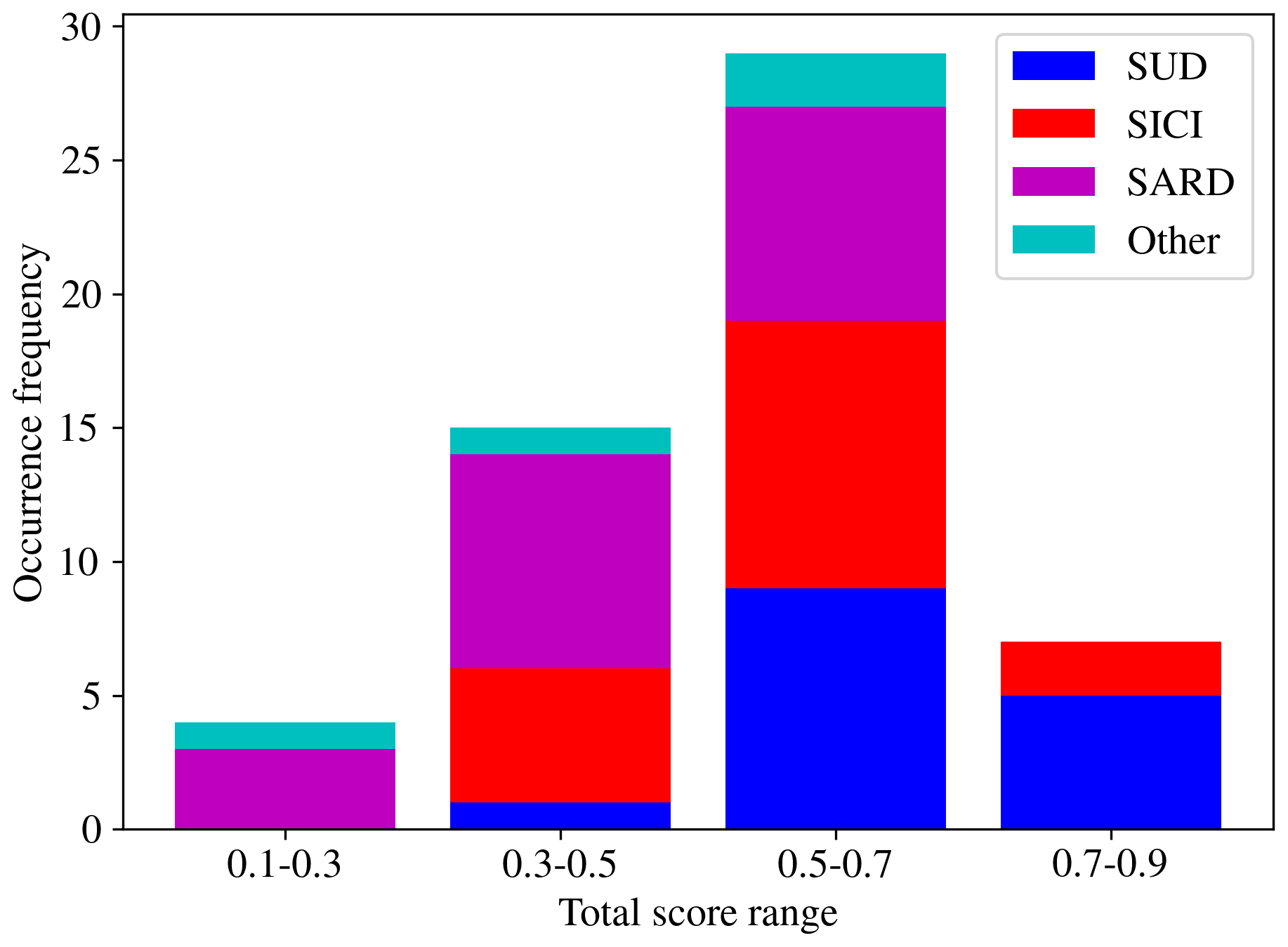
Figure 8 Occurrence frequency of various challenge groups sorted with the associated TERNA zone.

The challenge group of the wind farm serves as a crucial parameter in studying the future offshore energy scenario in Italy. Each farm project is associated with a score that can be interpreted as the construction probability of the farm itself. However, it is unknown a priori what farms will be built, and only a probabilistic approach can be pursued at this stage. This can be accomplished by means of a Monte Carlo method, where the predicted power production is calculated by means of 5000 simulations based on the challenge group of each wind farm. In each simulation, a wind farm is constructed with a probability given by its total score (2). A random uniformly distributed number between 0 and 1 is generated for each farm project: if the random number is lower than the farm total score the wind farm will contribute to the renewable power generation, and vice versa. The approach is not aimed at identifying the wind farms which are more likely to be built: on the contrary, it includes all proposed projects with a generation probability which depends on their challenge level.

5 Wake losses and layout identification

One of the critical parameters for the results is the array efficiency, namely the ratio between the total power production (without transmission losses) and the power of a reference turbine (usually one of the most upstream turbines unaffected by other wakes) times the number of turbines, N. This normalization should isolate wake losses, although blockage losses (Segalini and Dahlberg, 2020) are invisible to this metric, as discussed by Segalini (2021). Blockage losses, being within a few percent for broad layouts, were not accounted for in the current analysis. On the contrary, wake losses are deemed relevant to be assessed, and in the present work they were computed by means of the Jensen wake model (Katic et al., 1987; Shakoor et al., 2016) with the wake superposition scheme described by Sebastiani et al. (2021). The wake expansion parameter was kept constant to k=0.04 as suggested by Sebastiani et al. (2021) and is typical for offshore installations. However, in order to utilize the Jensen wake model, it is essential to define the layout of the farm so that wake losses can be quantified. The wind farm layout identification requires the determination of the positions of turbines within a given area to maximize the power output. The geometrical features of the area where each wind farm is supposed to be built can be retrieved from the database 4COffshore (4C Offshore, 2024), along with its bounding polygon.

To obtain a preliminary layout configuration, a genetic algorithm was developed (Vose, 1999; Lambora et al., 2019). It is worth noting that this initial layout does not aim to be the best-performing configuration (especially given the specific analysis uncertainties such as the number and types of turbines chosen by each project, the project feasibility, and the available farm polygon coordinates that often present irregular shapes, adding complexity to the optimization problem). Each wind farm could be described by N wind turbines distributed uniformly with a constant spacing, L, between the turbines given by

$$\begin{array}{}\text{(3)}& L=\sqrt{{\displaystyle \frac{\text{area polygon}}{N}}}.\end{array}$$

While L is a simple estimate of the spacing, the irregular shape of the polygon makes the layout identification challenging, motivating the use of an optimization algorithm such as the chosen genetic one. The farm area was subdivided into about 2000 allowed turbine positions uniformly distributed, and the optimization problem is the identification of the N positions that maximize the fitness function. While in general the fitness function is associated with the annual energy production (AEP) of the farm and the wind rose, here it was preferred to maximize the minimum distance between each turbine pair, due to the tight correlation between wake losses and intra-turbine distance and the rapidity of the fitness function calculation. Since the focus of the work lies in portfolio-scale and system-level analysis of offshore wind deployment, rather than in site-specific wind-farm layout optimization or bankable energy assessment, we consider that a synthetic and approximate layout obtained with geometric considerations might be appropriate. The goal of the layout identification is only to assess an approximate value of wake losses to be used later on in the Monte Carlo simulations.

In the genetic algorithm developed, a pool of 2000 randomly picked turbine layouts was created and the fitness function was computed for each pool member (namely a possible farm layout). Crossover between two binary-encoded members took place at a random crossover location (Mitchell, 1998). The reproduction ability of each member was associated with its fitness function, so that layouts with larger minimal intra-turbine distance had better chances to be used in the evolution. A 10 % probability of mutation (Mitchell, 1998) was also allowed in the encoded solutions to maintain genetic diversity. Finally, elitism (Mitchell, 1998) was introduced at every iteration by keeping the best two pool members untouched. The simulation is terminated after a given number of iterations (arbitrarily chosen to 500N, so that large farms required more computational time).

An example of the evolution process is shown in Fig. 9 for the Nereus wind farm near Puglia. N=120 turbines have been located within the intended polygon. The algorithm searches over 60 000 iterations and a rapid increase in the intra-turbine distance is observed within the first 5000 iterations, after which the increase becomes slower. The final best configuration had a minimal intra-turbine distance, L_opt, slightly larger than 1200 m, 20 % lower than the uniform value L=1526 m based on the polygon-enclosed area (3). The resulting layout shows that some turbines are further apart than others, underlining that the layout identified after so many iterations is suboptimal. At the same time, if some turbines are closer, some others will be more apart, so that the array efficiency should be similar to the optimal layout with uniform intra-turbine distance.

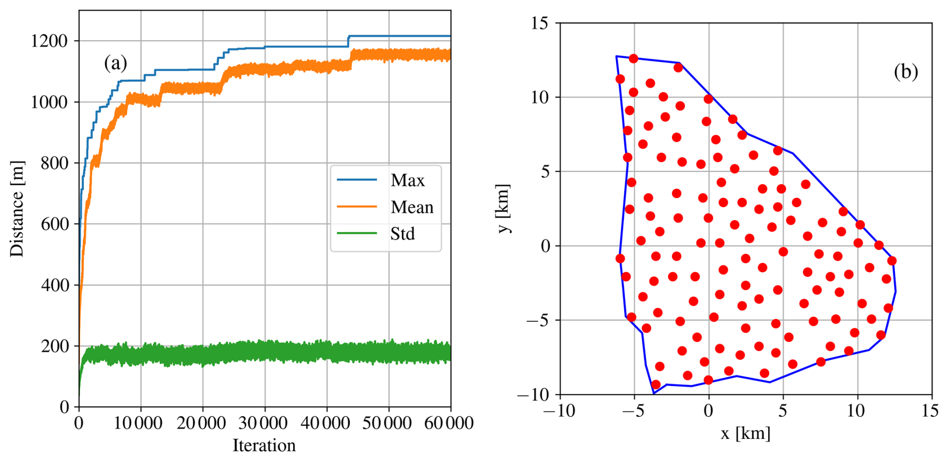
Figure 9 (a) Example of the evolution of the minimum intra-turbine distance in the genetic algorithm for the Nereus wind farm (120 turbines) for the optimal member, population average, and population standard deviation. (b) Final layout of the Nereus farm after 60 000 iterations.

The comparison between the uniform spacing, L, and the result of the optimization process, L_opt, is shown in Fig. 10 for all the considered farms. In general, the spacing resulting from the optimization algorithm is similar to (but slightly lower than) the uniform estimate, although some exceptions are also present for layouts with a small number of turbines (less than 25) where the optimization algorithm converges towards a spacing larger than the uniform solution (3).

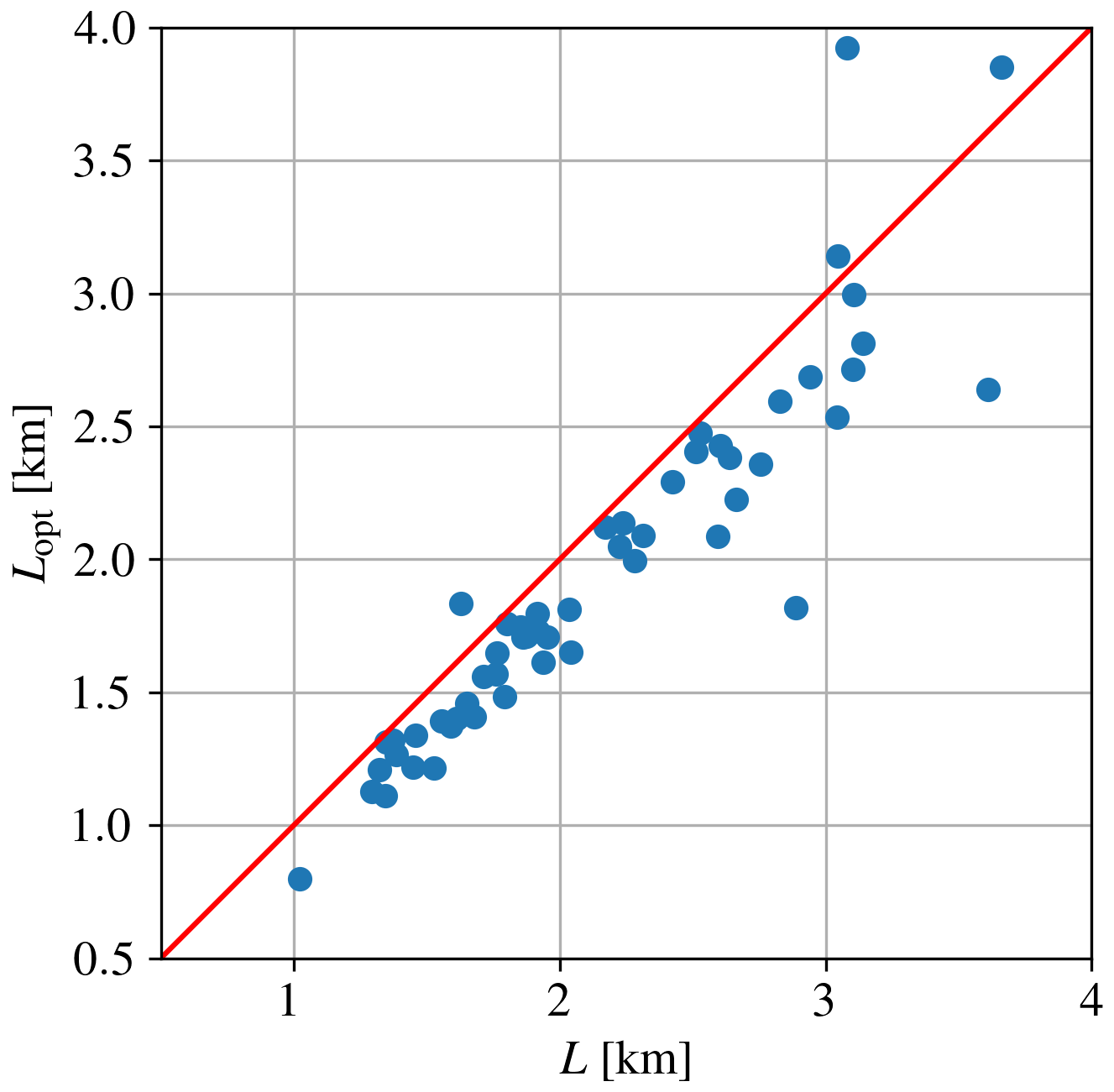
Figure 10 Minimum intra-turbine distance from the genetic algorithm, L_opt, plotted against the uniform distance estimate, L.

Considering that modern wind farms show spacings on the order of 8 turbine diameters, an intra-turbine distance of 1900 m should be recommended to limit wake losses. Several wind farms are characterized by spacings lower than ideal (in one case down to 1 km, namely 4 turbine diameters): this implies that wake losses might become significant in some cases. One could argue that such a tight spacing is a result of our choice of the IEA 15 MW turbine with a large turbine diameter, D=240 m. However, this is incorrect, since smaller turbines will have a lower rated power, necessitating a larger number of turbines to achieve the planned farm capacity. It is therefore expected that the ratio $L/D$ will remain almost constant regardless of the choice of the installed turbine. Typical spacings would generally be on the order of 5 to 7 rotor diameters and pushed to 8–10 rotor diameters for strongly unidirectional wind regimes only.

Having a preliminary layout from the genetic algorithm, the array efficiency was computed by means of the Jensen model (Katic et al., 1987; Sebastiani et al., 2021) from the historical time series of the wind velocity magnitude and direction. In general, the array efficiency depends on wind direction and wind speed. However, in the present project, the array efficiency has been averaged over all wind directions to enable rapid calculations over the long historical time series (31 years of hourly data). Figure 11 shows the collection of the array efficiency curves for all the considered farm projects. The structure of these efficiency curves is quite similar, with nearly constant low efficiency between cut-in and rated wind speed (at around 10–11 m s⁻¹) and high efficiency near 1 sufficiently above the rated speed. As expected, the low efficiency value is associated with low intra-turbine spacing and follows an increasing curve function of the farm spacing (Fig. 11b). Furthermore, Fig. 11b can be used to rapidly assess the array efficiency of the farm even without an optimization procedure: by using the theoretical L value (based on just the bounding polygon area and number of turbines installed), it is possible to rapidly estimate the array efficiency below rated wind speed by interpolating through the orange points, obtained by plotting the identified optimal layout array efficiency (in the ordinate) against the L parameter.

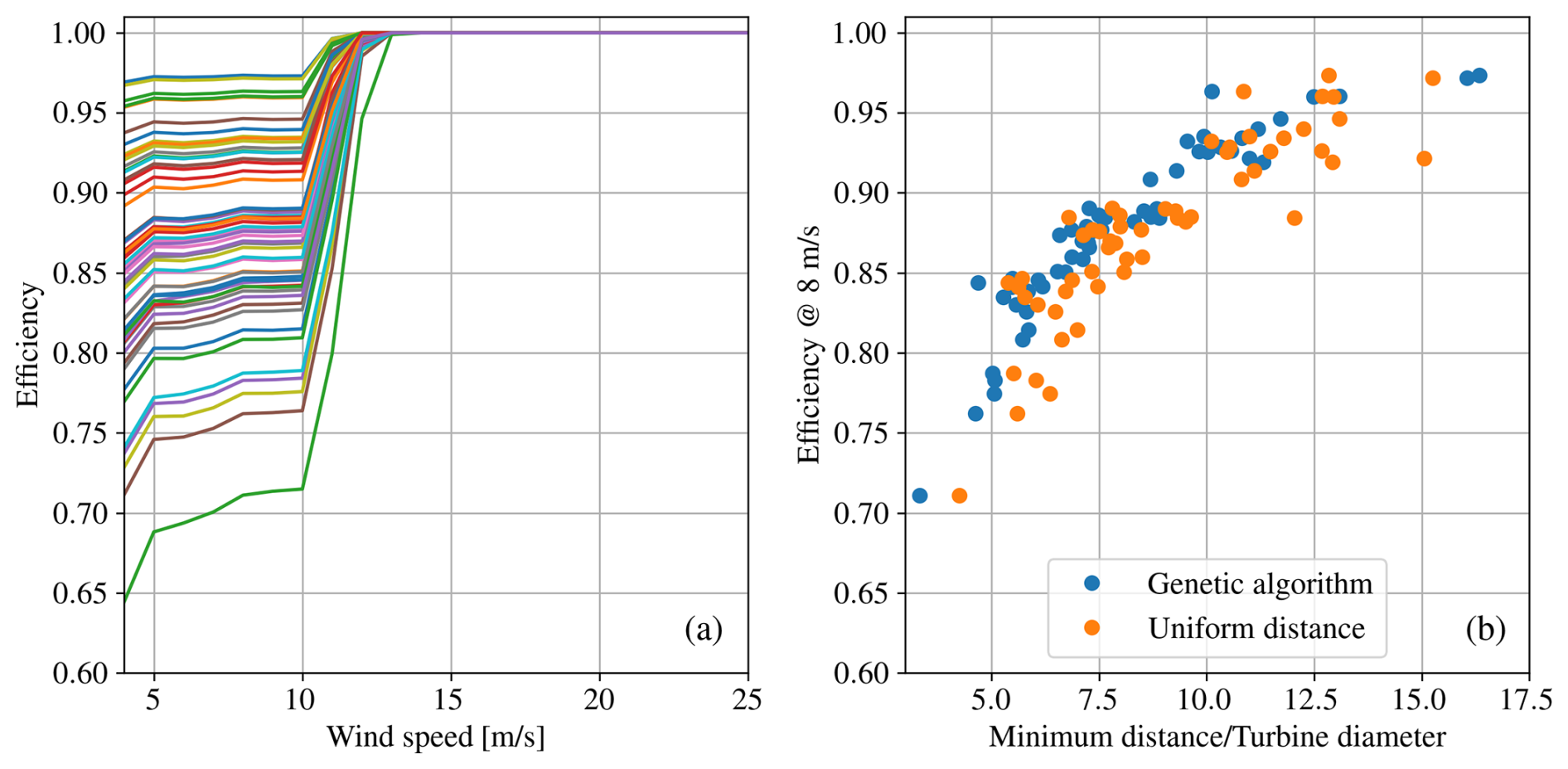
Figure 11 Array efficiency for all the considered wind farms. (a) Azimuthal average of the array efficiency. (b) Efficiency at 8 m s⁻¹ plotted against L_opt or L normalized by the turbine diameter.

A validation of the adopted layout identification has been performed on the existing Lillgrund offshore wind farm used in several investigations (Sebastiani et al., 2021). Having available the bounding perimeter and the number of turbines to be installed (48 Siemens 2.3 MW with diameter 93 m), the optimal layout, able to maximize the minimum distance between the turbines, was identified by means of the genetic algorithm without taking into account the wind rose. The identified geometry is shown in Fig. 12 together with the estimated array efficiency. While some discrepancies exist in the array efficiency, it is quite visible that the overall structure of the wake losses is well captured. The average array efficiency below rated speed is 0.616 for the Lillgrund setup (the latter is estimated by means of SCADA analysis from the Lillgrund wind farm; Sebastiani et al., 2021), while the identified layout shows a value of 0.622, namely slightly larger: this increase was expected, since the real layout has two turbines in the center of the farm that could not be installed because of an insufficient sea depth, an aspect not included in the present optimization scheme. A similar analysis has been performed for the Horns Rev 1 wind farm with similar qualitative agreement (not shown).

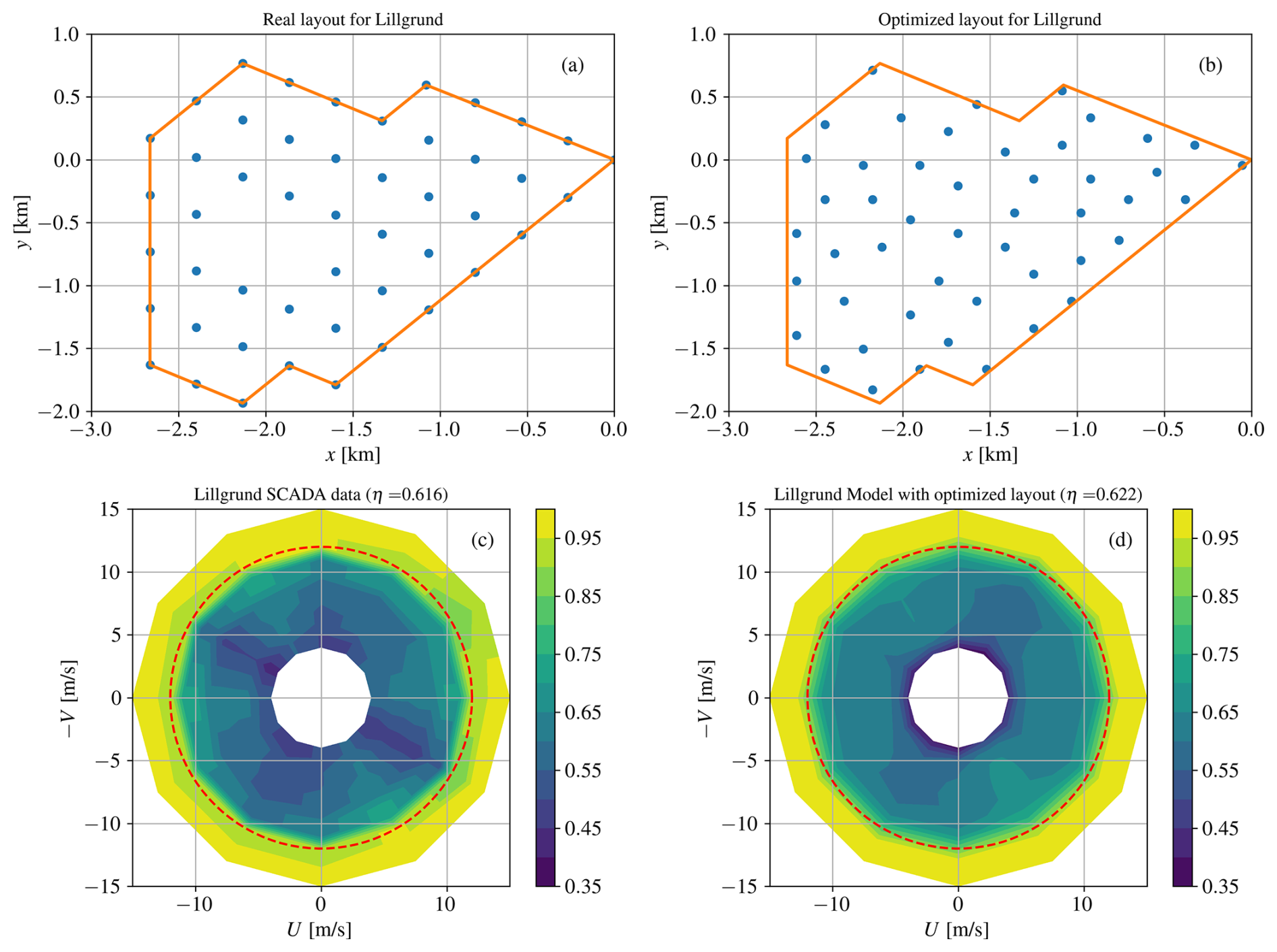
Figure 12 Validation of the optimization method for the Lillgrund wind farm. (a, b) Layout of the farm; (c, d) array efficiency for different wind velocities and directions (the dashed red line indicates the rated speed of the installed Siemens wind turbine, 12 m s⁻¹). (a, c) Real Lillgrund data (Sebastiani et al., 2021); (b, d) analysis of the optimized layout with the minimum distance fitness function. The title of the bottom row reports the average array efficiency of the farm for velocity below rated speed.

6 Monte Carlo results

In a Monte Carlo simulation, the possible outcome of building wind farms is modeled by using random variables to represent the challenging construction process. The simulation generates a large number of random samples to explore the possible outcomes of the system under different conditions. Each farm layout will experience the associated historical velocity time series, so that the randomness remains only on whether or not each farm will be constructed. If the wind farm is operated, it will start producing power due to the wind availability. Wake losses will be accounted for by means of the array efficiency computed in Sect. 5, while transmission and other generic losses are included by decreasing the overall production with a factor of 15 %.

The simulation estimates the total power production for each TERNA market zone from multiple simulations. This provides insights into the potential production capacity of wind farms under different scenarios. The results of 5000 Monte Carlo simulations are shown in Fig. 13, where the averaged power production is shown in the case where all farms are constructed and in the average case from the possible Monte Carlo scenarios. Three main TERNA zones are associated with the highest production, namely SUD, SICI, and SARD. A significant decrease between the planned and most probable wind farms is observed, with a decrease on the order of 40 %. The standard deviation obtained from the Monte Carlo is also shown, highlighting the variability range of the simulations.

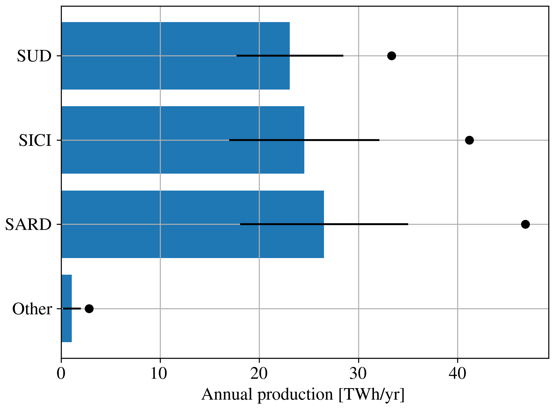
Figure 13 Annual power production in the various Italian zones. Black circles: power production when all farms are approved. Blue bars with error bars: expected value of the power production with the associated standard deviation as error bars.

By looking at the global numbers, all 55 farm projects sum up to almost 3100 turbines for a global installed capacity of approximately 46 GW (namely 406 TWh yr⁻¹ assuming a capacity factor of 100 %). However, by just considering the historical time series, only 158 TWh yr⁻¹ is actually produced, a number that decreases to 146 TWh yr⁻¹ when wake losses are accounted for and to 124 TWh yr⁻¹ when other losses are included. The results of the Monte Carlo show instead that the latter number decreases to 76 TWh yr⁻¹ due to the fact that some wind farms are more challenging than others and, therefore, are considered to statistically contribute less to the overall portfolio production. This result is 3 times the 2023 TERNA production scenario of 24 TWh yr⁻¹ required to meet the Fit For 55 (FF55) European target (TERNA, 2023). It can be evinced that, based on the current simulation and challenge parameters, the license to build should be granted to at least one-third of the portfolio (i.e., 14 GW of projects) to aim for a successful delivery of 24 TWh yr⁻¹ into the grid by offshore wind power.

Figure 14 shows the power production contribution for each month for the three highest-producing TERNA market zones. It is clearly visible that winter months are the ones associated with the largest energy production, while summer months are associated with the lowest wind energy production. The variability is the least for the SUD TERNA zone (namely Puglia), but the trend is consistent between the three zones otherwise.

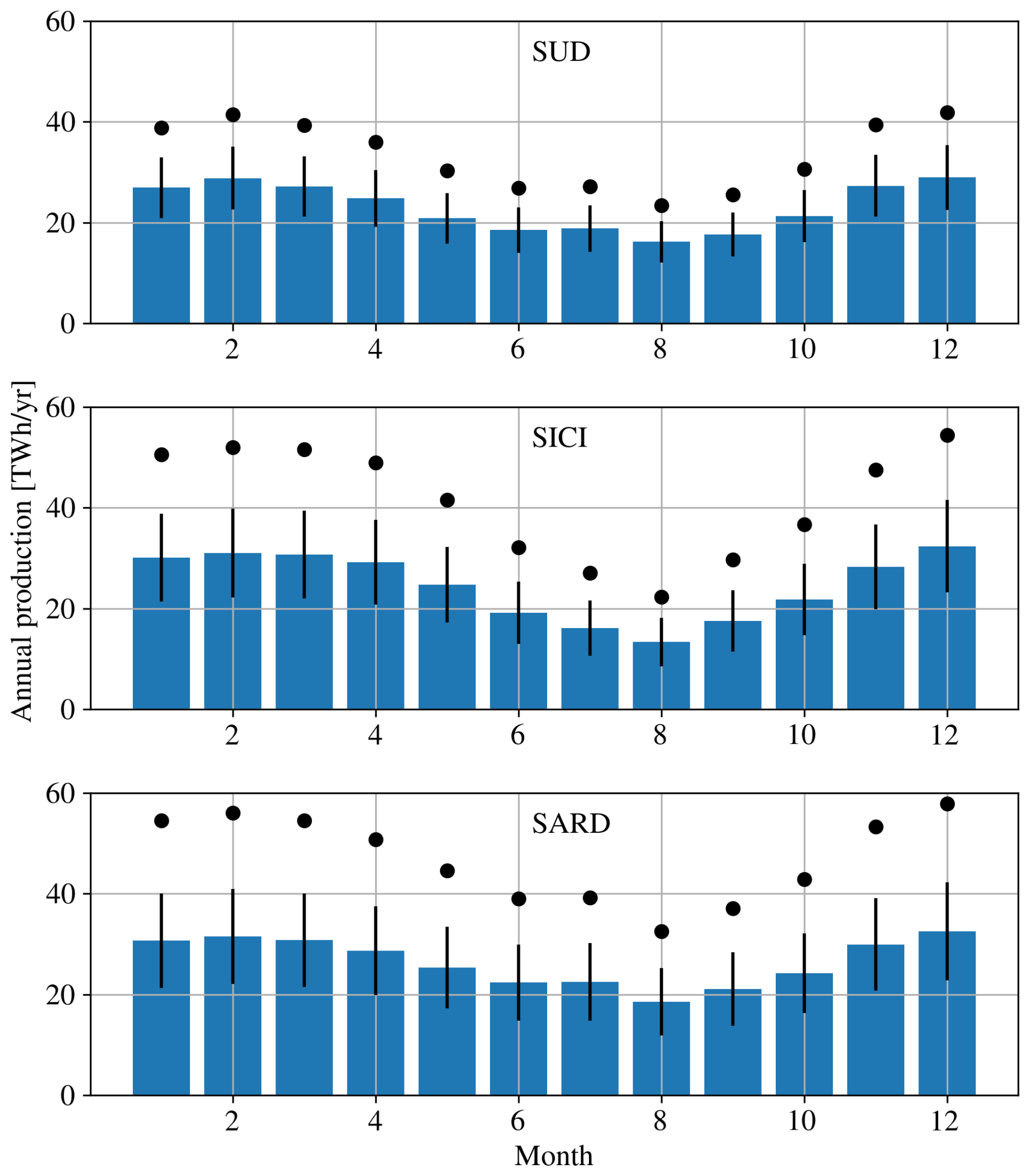
Figure 14 Annual power production in the three highest-producing Italian zones, i.e. SUD, SICI, and SARD, sorted for each month of the year. Black circles: power production when all farms are approved. Blue bars with error bars: expected value of the power production with the associated standard deviation.

The current study is effectively a central analysis of the possible production from a portfolio of wind farms; i.e., it represents a P50 production split by macro-areas. The uncertainty should be addressed on a portfolio basis, hence deviating from the typical uncertainty approach of energy assessments. The reason is that each wind farm is considered to be a single production source simulated in operation in different wind regimes. Typical uncertainty sources such as wind-flow modeling, power curve, and wake modeling should all therefore be allocated under a “production uncertainty”, which is, however, not the aim of this work. The reason is that we focus on the system rather than on the single production unit. On the other hand, windiness and the uncertainty related to the CERRA database have a direct effect on the production of the system. It is therefore believed that this should be considered the relevant uncertainty source for this study.

7 Conclusions

The development of offshore wind farms in Italy is rapidly evolving, with clear interest in succeeding and to meet the increasing demands of renewables in Europe. However, success requires high investments on the order of millions of euros just to prepare an initial project and requires significant technological development for the predominantly floating projects. Authorities also need to facilitate the transition not only with the recently approved FER2 Decree and the EUR 185 MWh⁻¹ tariff granted to offshore wind, but also with continuous efforts and support. Knowledge of possible scenarios can help the stakeholders in making informed decisions. In this respect, the authors have studied the statistical contribution that more than 46 GW of offshore wind farms, selected within those under development in Italy, can bring to the energy production. The 55 projects can be considered a representative sample of the overall 90 GW connection requests submitted to TERNA. The basis of the analysis is the IEA240-15MW wind turbine model, which shows characteristics in line with top-class offshore wind turbines on the market. By identifying simplified layouts within each area under development based on geometric considerations only, and after accounting for all losses, the typical capacity factor across the Italian offshore areas is shown to be generally between 30 % and 40 %. These values are higher than onshore wind farms, and the access to available areas is a key benefit; however, the associated costs with floating offshore wind energy could make the business models particularly demanding. We assume that all 55 proposed wind farms can produce energy, with some projects, however, more capable of capitalizing on the combined parameters selected for the study, as demonstrated by the Monte Carlo simulation. The scoring system is based on wind speed, sea depth, installed capacity, and distance to the coast. As an example, it is reasonable that a higher sea depth will require greater efforts to adapt the floater, chains, and dynamic cables and obviously to manage the associated costs. The total score estimated in this study shows that the TERNA areas proposed for the connection of the offshore projects are reasonably balanced in terms of production, although projects in Sicily and Puglia can benefit from their lower sea depth. On the other hand, the time lag between Sardinia and Sicily might offer an interesting trade-off between the challenges faced in development and the energy injected into the grid.

If all 55 projects are built (43.4 GW), the production is estimated to be 124 TWh yr⁻¹. If the Monte Carlo simulation is considered in order to estimate a challenge probability of success, the production is estimated to be 76 TWh yr⁻¹, which means that approximately 60 % of the projects have statistical significance to overcome the four technical challenges combined. If we target 24 TWh yr⁻¹ of production with offshore wind to meet the FF55 goal (the TERNA scenario), the license to build should be granted to at least one-third of the portfolio, i.e. 14 GW. By this approach, the authors consider that there is statistical significance that the production target can be met.