Characterizing atmospheric stability in complex terrain

Characterizing atmospheric stability becomes challenging in heterogeneous, complex terrain. We use data from 47 meteorological towers associated with the Perdigão field campaign to recommend data-processing approaches and to assess the limitations of shorter or fewer towers. We quantify atmospheric stability according to the Obukhov length, the turbulence kinetic energy, and the turbulence dissipation rate using two decomposition periods, including consistent 10 min periods to match convention in the wind energy community and consistent 30 min periods to match convention in the atmospheric science community. We also demonstrate a methodology that can indicate the necessary number and location of towers to characterize atmospheric stability. We find that the 10 min Reynolds decomposition window underestimates turbulence patterns. Additionally, 10 m measurements do not provide reliable 100 m hub-height stability predictions. Holistically, this work addresses challenges in relying on sparse surface measurements.

1 Introduction

The atmospheric boundary layer (ABL) directly interacts with Earth's surface, and the surface–atmosphere interactions that occur in this layer dictate transport of heat, momentum, sediment, and moisture into the larger atmosphere (Stull, 1988). Understanding these exchange processes has implications for fields like renewable energy (Pérez Albornoz et al., 2022) and agriculture (Tang et al., 2022). These exchange processes are also highly dynamic and sensitive to atmospheric stability (Garratt, 1994).

Atmospheric stability controls how the atmosphere responds to disturbances, affected by buoyancy and/or mechanical forcing. Static stability considers how buoyancy or temperature gradients may affect a vertically perturbed air parcel. A region of the atmosphere is statically stable if a perturbed parcel in that region experiences restoring forces toward its equilibrium height, statically unstable if the air parcel rises away from its equilibrium height, and neutral if the air parcel is unaffected. Dynamic stability considers the effects of both buoyancy and wind shear processes to determine whether a flow will become turbulent. Statically stable flows can be dynamically unstable and can become turbulent if the wind shear is strong enough. Thus, laminar flow exists only if the layer of air is stable both dynamically and statically (Stull, 1988; Angevine et al., 2020). Atmospheric stability characterization remains an active field of study for fields like wind energy (Pérez Albornoz et al., 2022).

Atmospheric stability affects wind power generation through the effects of turbulence, shear, and veer. In very early work, Elliott (1990) showed that significant errors in power curve measurements can result if the stability-influenced effects of wind shear and turbulence are ignored. Wharton and Lundquist (2012) showed that stable conditions led to turbine overperformance. At a different, high-plain location, Vanderwende and Lundquist (2012) found that stable conditions were associated with reduced power performance. Similarly, Bardal et al. (2015) found reduced power in the middle of the power curve for cases with shear exponents greater than 0.15 for a coastal site. At a flat-terrain site, Gao et al. (2021) found that the shape of the wind veer profile affects differences in power performance. Sanchez Gomez and Lundquist (2020) studied power production at an onshore wind power plant in flat terrain and found that, while large values of wind veer were associated with turbine underperformance, large shear values with small values of wind veer were associated with turbine overperformance, resolving the apparent contradiction between Wharton and Lundquist (2012) and Vanderwende and Lundquist (2012).

The stability-driven effects of turbulence, wind shear, and wind veer also affect turbine loads. Sathe et al. (2013) showed that rotor and tower loads increase in high-shear environments at both flat and ocean sites. Further, in Dimitrov et al. (2018), while wind shear was shown to strongly influence blade root loads, veer showed only a minimal effect on fatigue loads for flat, forested, and mountainous sites. Wind shear also dominated the sensitivity analysis performed in Robertson et al. (2019), with 18 different parameters influencing blade root out-of-plane pitching moments and blade shaft bending moments. Putri et al. (2019) found that the fatigue damage of a spar-buoy offshore wind turbine is higher in unstable cases than in near-neutral cases.

Atmospheric stability also affects turbine wakes. Baker and Walker (1984) observed a slower wake recovery for a wind turbine under stable conditions for a mountainous, forested site. Magnusson and Smedman (1994) showed a larger velocity deficit in stable conditions for a turbine in coastal conditions. Iungo and Porté-Agel (2014) also showed a faster wake recovery under convective conditions for a valley site surrounded by mountains. The scanning lidar measurements of Aitken et al. (2014), taken at a flat site downwind of complex terrain, also found slightly stronger wake deficits in stable conditions even for a turbulent site, while the scanning lidar measurements of Bodini et al. (2017) for a flat site in Iowa showed that wakes persist further in stable conditions. Wind turbine wakes also respond to the stability-driven effects of wind veer. Large-eddy simulation studies (Vollmer et al., 2016; Churchfield and Sirnivas, 2018), scanning lidar measurements (Bodini et al., 2017), and nacelle lidar measurements (Brugger et al., 2019) have shown that in the veering flow typical of stably stratified conditions, the wake will stretch into a three-dimensional ellipse. Englberger and Dörnbrack (2018) showed that increasing veer increases the erosion of the turbine wake in both flat and complex terrain. Stability-based effects on wake propagation also have secondary effects on turbine power generation (Barthelmie et al., 2013). Keck et al. (2014) compared the results of their dynamic wake meandering model to field observations and showed 22 % differences in wake losses between stable and unstable conditions.

Given that atmospheric stability has implications for power generation, turbine loads, and wake propagation, determining optimal atmospheric stability definitions is critical for reliable wind resource assessments and wind energy forecasting (Optis and Perr-Sauer, 2019; Lee et al., 2020). However, multiple metrics exist to quantify stability. Some metrics, like the Obukhov length (Monin and Obukhov, 1954), classify stability at a single altitude. Other metrics, like the bulk and gradient Richardson numbers, classify stability across a given vertical extent, while turbulence kinetic energy (TKE) and turbulence dissipation rate (ϵ) characterize stability indirectly through turbulence (Stull, 1988). Some metrics also rely on determining an appropriate averaging window, and there are multiple, sometimes conflicting, approaches for defining the averaging window (Howell and Mahrt, 1994).

Financial constraints also inform challenges to atmospheric stability characterization. While meteorological towers can provide both the wind and the temperature measurements required to assess atmospheric stability, the material costs for meteorological towers alone can cost of the order of USD 1 million for a 100 MW utility-scale onshore project (Eberle et al., 2019). Sonic anemometers to measure wind characteristics and thermometers to measure temperatures introduce additional costs. Thus, it could be possible to reduce costs if surface stability assessments were more reliable in predicting hub-height stability without the need to invest in tall (i.e., 100 m) meteorological towers.

Complex terrain introduces further challenges to atmospheric stability classification (Serafin et al., 2018; Cantero et al., 2022). Skillful wind forecasts in complex terrain are challenging, owing largely to the prevalence of heterogeneous, terrain-modulated flows, such as mountain wakes, mountain waves, gap flows, valley cold pools, and mountain-valley circulations (Fernando et al., 2019). Despite these issues, many modeling efforts still rely on physical parameterizations developed over flat, horizontally homogeneous terrain because of constrained data availability (Stiperski and Rotach, 2016; Sfyri et al., 2018).

These complex-terrain dynamics influence wind energy siting and further complicate wind energy assessments (Clifton et al., 2022). Lange et al. (2017) used a scale model in a three-dimensional wind testing chamber and showed that the mean wind, wind shear, and turbulence level are extremely sensitive to the exact details of the terrain, affecting the lifetime and maintenance costs of wind turbines. Han et al. (2018) found that complex terrain modifies wind profiles, resulting in significant performance differences under both stable and unstable conditions. Despite their impact, these dynamics are still not captured well by commonly used commercial wind farm planning models (Shaw et al., 2019; Olson et al., 2019).

The Perdigão field campaign (Fernando et al., 2019) provided a comprehensive dataset for studying flow in complex terrain. Extensive instrumentation across the Vale do Cobrão enabled new insights into recirculation, gustiness, low-level jets, and mountain waves, as well as wind-energy-relevant phenomena such as wake deflection and wake self-similarity, as discussed in detail below. The Perdigão measurements have also supported major advances in modeling, including a long-term Weather Research and Forecasting (WRF) large-eddy simulation (LES) simulation, improved terrain and canopy representations, turbulence-initiating CPM approaches, and virtual-lidar emulation. In parallel, Perdigão spurred development of multi-lidar scanning strategies and virtual-tower methods that extend measurement capabilities aloft.

Despite these advances, existing Perdigão analyses share two important limitations. First, most focus on vertical extrapolation, virtual towers, and rotor-layer prediction, while largely neglecting how horizontal heterogeneity imposed by steep terrain and vegetation modulates near-surface flow. Second, although technological solutions have enabled reliance on measurements above 40–80 m, the representativeness of surface or 10 m observations remains poorly understood. This gap directly affects wind energy stakeholders, who often depend on near-surface measurements for resource assessment and may be unable to deploy tall towers in complex terrain.

These limitations motivate the present study. We evaluate the representativeness of Perdigão’s 10 m surface measurements using three stability metrics and assess their ability to capture temporal variability, vertical structure, and terrain-driven heterogeneity. The resulting guidance informs both meteorological analysis of complex terrain and practical tower-siting decisions for wind energy applications. Section 2 describes the field campaign, data preparation, and metrics; Sects. 3 and 4 present and discuss the results; and Sect. 5 concludes with recommendations.

2 Data and methods

2.1 Perdigão field campaign

The Perdigão field campaign, which occurred from 1 May–15 June 2017, was a scientific research effort near the town of Perdigão in central Portugal. This international collaboration addressed knowledge gaps surrounding the microscale details of winds in complex terrain by collecting a comprehensive, high-resolution dataset of meteorological quantities for the site (Fernando et al., 2019). The field campaign took place in the Vale do Cobrão, with an approximately two-dimensional valley and parallel ridges with annual 10 m wind climatology perpendicular to the ridges (Fig. 1).

Perdigão addressed fundamental understandings of physical mechanisms in complex terrain. Menke et al. (2019) documented recirculation zones throughout the valley with Doppler radar data. Letson et al. (2019) used data from both sonic anemometers and Doppler lidars to assess wind gust characteristics. Wagner et al. (2019), Wildmann et al. (2019), and Venkatraman et al. (2023) analyzed detection of low-level jets (LLJs). Wise et al. (2022) documented mountain wave patterns, which were further studied by Robey and Lundquist (2024). This field campaign has also supported research into wind-energy-specific processes like wind turbine wakes. Menke et al. (2018) used data from six scanning lidars to analyze the dependence of wake deflection patterns on atmospheric stability, and these wake deflection patterns were also scrutinized by Barthelmie and Pryor (2019) and Wise et al. (2022). Similarly, Dar et al. (2019) simulated the wake behind a turbine and showed that the self-similarity of the wake implied that the wake pattern depended on neither the complexity nor the shape of the terrain.

Improving the understanding of these physical mechanisms has also enabled model improvement. Wagner et al. (2019) established a foundation with a long-term, albeit coarse, Weather Research and Forecasting (WRF) large-eddy simulation (LES) simulation set for the full observational period. Palma et al. (2020) developed a digital terrain model (DTM) for the site and also defined the necessary horizontal grid cell spacing criteria of 40 m to appropriately characterize the site. Several modeling works have also expanded upon this need for improved representation of horizontal variability for the region. Quimbayo-Duarte et al. (2022) established a forest canopy parameterization for the WRF-LES model that improved wind modeling within the lowest 500 m of the atmosphere and attributed the imposed drag parameterization to a need for even higher-resolution land surface inputs. Venkatraman et al. (2023) altered the forest canopy parameterization to consider more realistic (i.e., shorter) heights in a set of OpenFOAM simulations. Finally, Al Oqaily et al. (2025) – building upon the ensemble models in Giani and Crippa (2024) – again underscored the importance of land cover in an additional set of LESs. Connolly et al. (2021) demonstrated the utility of the cell perturbation method (CPM) (Muñoz-Esparza et al., 2015) in capturing flow features in LESss of the region, especially in weakly convective conditions. The Perdigão field campaign has also enabled improvements in wind-turbine-specific modeling in complex terrain. Wise et al. (2022) introduced the WRF-LES-GAD to the Perdigão dataset, and leveraging the output from this model, Robey and Lundquist (2024) demonstrated the utility of a virtual lidar model (Robey and Lundquist, 2022) in simulating range height indicator (RHI) scans. The modeling improvements have also extended beyond numerical weather prediction (NWP) models. Barthelmie and Pryor (2019) developed a novel detection algorithm that could both identify and characterize wake patterns, Vassallo et al. (2020) used artificial neural networks (ANNs) to improve wind speed error by up to 52 %, Bodini et al. (2020) used machine-learning models to reduce the average error in model representation of the turbulence dissipation rate by up to 40 %, and Mosso et al. (2025) predicted turbulence anisotropy for the region using random forest models.

The Perdigão field campaign has also enabled improvements in measurement techniques. Vasiljević et al. (2017) outlined a methodology for multi-lidar Doppler lidar experiments, and Wildmann et al. (2019) presented a new wake measurement strategy that used three synchronized lidars to adapt to the prevailing wind direction automatically. Bell et al. (2020) combined multiple Doppler lidar scans to create virtual towers that could extend beyond the range of traditional in situ meteorological towers. Coimbra et al. (2025) also performed a virtual mast analysis of the Perdigão region with three coordinated dual lidars. These measurements allowed for not only the mean quantity comparisons available in Bell et al. (2020), but also turbulent quantities.

2.2 Perdigão field campaign measurements

Multiple instruments were deployed throughout the field campaign. Instrumentation included 49 meteorological towers, radiosondes, lidars, 2 tethered lifting systems, and additional instrumentation (including radars and radiometers) (Fernando et al., 2019).

The meteorological towers provide the main data source for this analysis. A total of 47 of the 49 towers included a 20 Hz sonic anemometer at the 10 m (“surface”) level. Of these 47 towers, 18 also included a 1 Hz thermometer at this 10 m level, although the only 10 m temperature measurements that were used for this analysis were from the three 100 m towers. All towers were constructed to minimize flow distortion by the tower. In cases where local obstacles interfered with the anemometer location, the anemometer boom was set to point down-valley. Booms on the towers pointed toward directions varying between 111 and 166°. The azimuth, pitch, roll, and height of the sonic anemometer mounting booms were measured and recorded. The sonic anemometer data were then tilt corrected using the planar fit method following the approach of Wilczak et al. (2001).

The three 100 m towers were strategically placed to sample flow conditions within differing terrains. Specifically, tse04 was located on an exposed ridge on the southwest, tse09 in the valley with eucalyptus and fir trees, and tse13 on a ridge with a heterogeneous canopy to the northeast (Table 1). Although translating CORINE Land Cover data (Bossard et al., 2000) into US Geological Survey land use types to obtain surface roughness lengths (Pineda et al., 2004) suggests surface roughness lengths of the order of 0.01–0.05 m, Wise et al. (2022), Wagner et al. (2019), and Palma et al. (2020) (among many others) have suggested that larger surface roughness lengths are more appropriate for the site. The mean canopy heights – as documented in Letson et al. (2019) – are below 10 m (Table 1 and Fig. 2), although individual trees may extend to 15 m (Mosso et al., 2025). For each 100 m tower, 20 Hz sonic anemometers and 1 Hz temperature sensor measurements were collected at 10, 20, 40, 60, 80, and 100 m (Fernando et al., 2019; EOL, 2019), among other measurements. The 60 m temperature measurements for tse13 (NE ridge) were not used here due to their frequent (76 %) data unavailability.

Table 1 Short-name reference for 100 m towers.

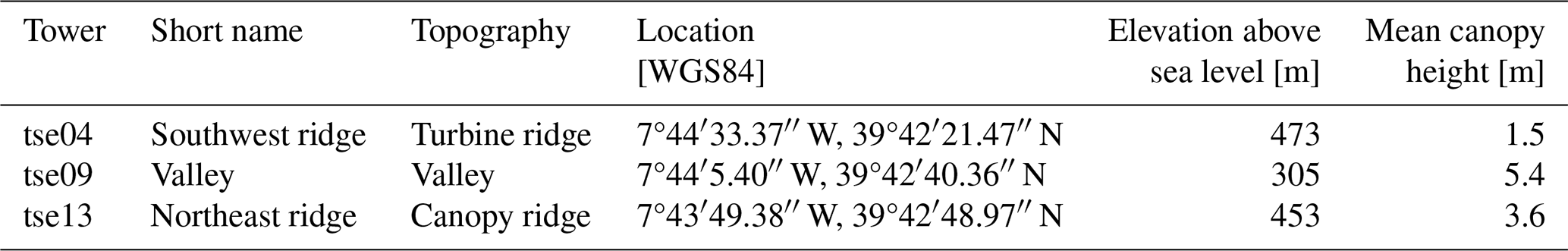
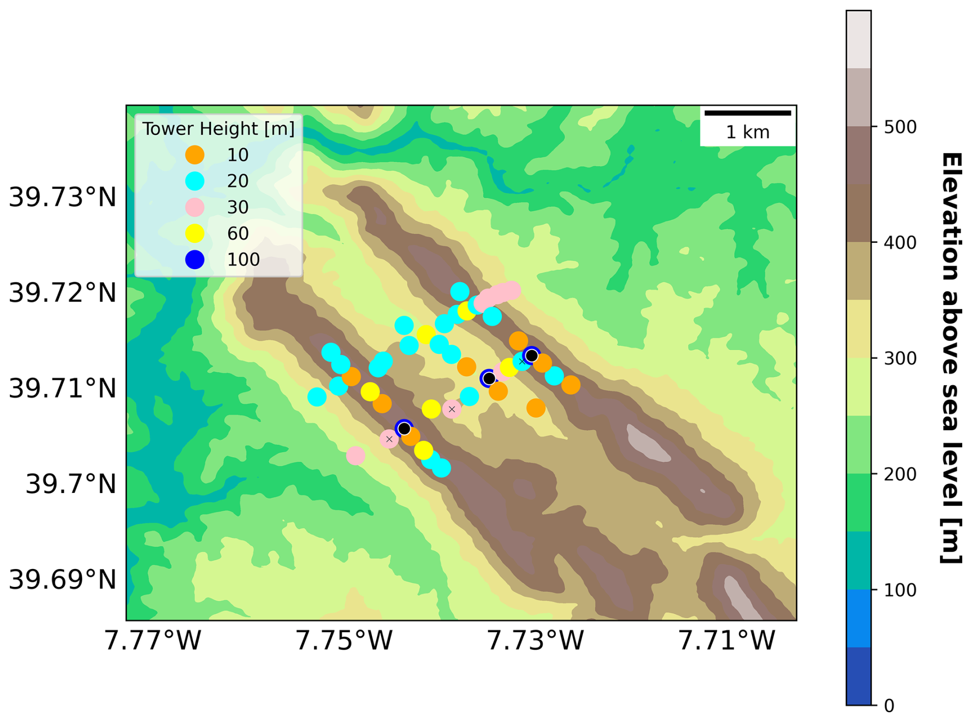
Figure 1 Topographic map of the Perdigão valley field campaign site with meteorological towers included. The 100 m towers are additionally marked with the black circle, and their corresponding radiometer measurements are indicated with the “X”. Other extensive instrumentation is not depicted.

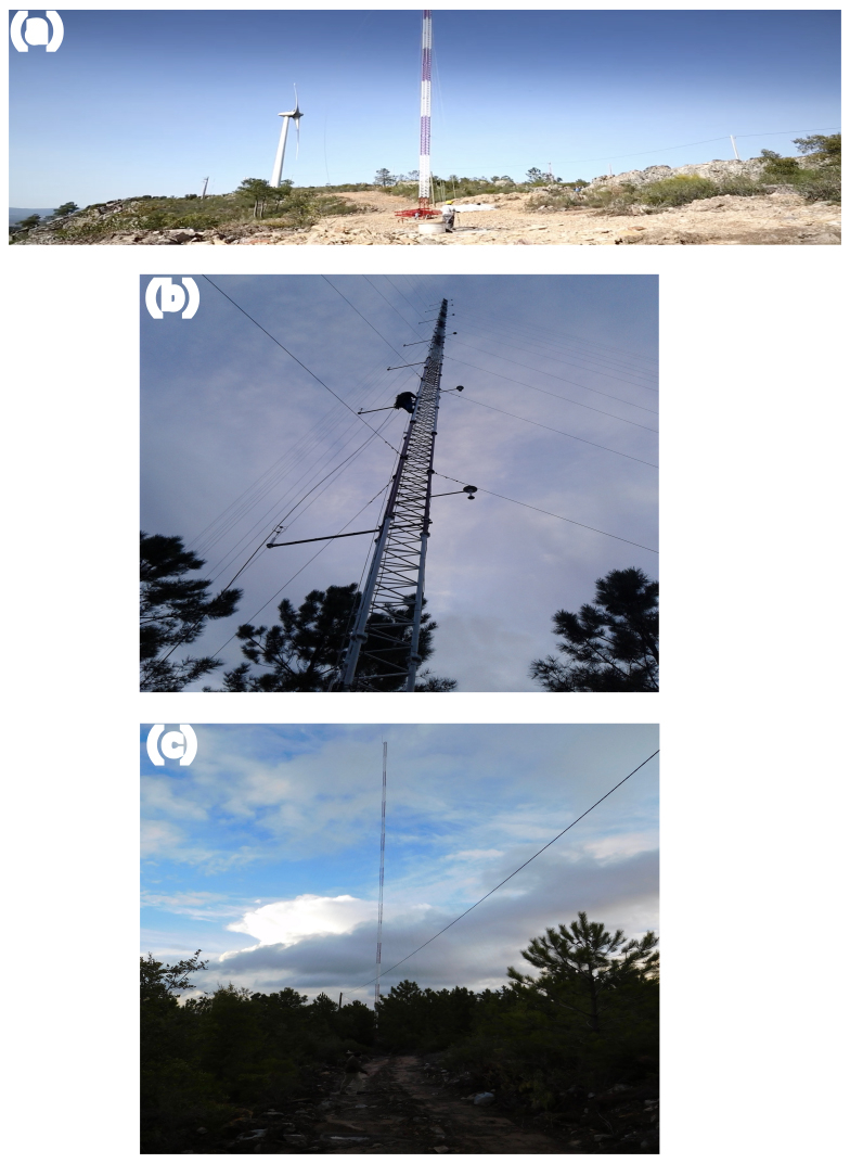
Figure 2 Canopy cover for (a) tse04, (b) tse09, and (c) tse13. The image of tse04 was identified as a still photo in the Danish Technical University (DTU) Perdigão video (DTU Wind and Energy Systems, 2017), and the images of tse09 and tse13 can be found in the Perdigão data archive (EOL, 2026).

2.3 Data preparation

The analysis presented herein relies on the 20 Hz sonic anemometer and 1 Hz air temperature sensor measurements from the meteorological towers (EOL, 2019). These data were also screened for quality control. Notably, data that suggested tower wake effects from the booms were removed within 60° (±30°) based on the process outlined in McCaffrey et al. (2017). These screening processes collectively removed 3.2 % of the 20 Hz data. Block-averaged fluxes (Babić et al., 2016; Wildmann et al., 2019) were then calculated using an eddy-covariance approach (Aubinet et al., 2012) from the surviving data for all heights using two different Reynolds decomposition times, discussed below in Sect. 2.3.5. The stability and turbulence metrics were calculated from these fluxes.

Two stages of screening were also performed to account for shading effects. First, data on days with clouds or precipitation were screened out of the analysis. The Perdigão field log (Supplement to Fernando et al., 2019) continues a daily breakdown of the synoptic conditions according to eight European standard patterns defined in Santos et al. (2016). This field log, along with determining the relevant synoptic regime for a day, also notes relevant weather patterns, such as cloud presence and precipitation. Based on this analysis, we screen out any days that include low or medium clouds as well as those with fog or precipitation. In situations where these weather patterns only affect targeted hours of the day, we remove the entire day to avoid biasing diurnal patterns. The net result of this screening is that 22 of the 45 d is removed (Appendix A).

Radiometer measurements informed the second, terrain-based shading screening. These measurements – located near the 100 m towers at tse02, tse07, and tse12 – were collected at either 20 m or 30 m and reported at 5 min intervals. These (cloudless, as defined above) incoming shortwave radiation measurements were diurnally-averaged and compared to the amount of incoming shortwave radiation expected by the Ineichen–Perez clear-sky model (Ineichen and Perez, 2002), as defined in the Python package pvlib (Anderson et al., 2023). The residual (measured–expected) was then assumed to trace hours where terrain shading might be assumed to occur. Instead of discarding data associated with shading, by identifying inequitable patterns in solar exposure between the towers, we were able to tailor our definitions of “stable” and “unstable” to only focus on hours that were not affected by these differences. Shown later, these stable and unstable hour definitions also inform our determination of an appropriate Reynolds decomposition window for two of the three stability metrics. Taken together, these two strict shading evaluations minimize spatial and temporal biases between towers and support a more equitable evaluation.

2.3.1 Metric selection

This analysis evaluates three stability metrics: the Obukhov length (L), turbulence kinetic energy (TKE), and the turbulence dissipation rate (ϵ). While many other stability metrics exist (Stull, 1988), this metric subset was selected to include a mix of both categorical and qualitative metrics and only metrics with a strong and consistent diurnal cycle.

The mix of categorical and qualitative metrics provides a means to categorize stability behavior based on regime. For example, because the Obukhov length categorically represents atmospheric stability (i.e., stable vs. unstable), we can compare the values of another stability metric (TKE, for example) during periods where the Obukhov length is stable with those during periods where the Obukhov length is unstable.

The diurnal cycle restriction was designed to assess how well the metric captures diurnal variability in boundary layer behavior. For L, each period was classified with a stability based on Table 2. Then, for each hour of the day, the total number of cases for each stability bin was summed and then normalized by the total number of cases for that hour throughout the experiment. The TKE and ϵ diurnal cycles were analyzed as diurnal distributions. For all metrics, the diurnal test was applied to the data from the surface (10 m) and aloft (100 m) separately and evaluated qualitatively. Turbulence intensity, which is another common metric in the wind energy community, was shown to have a variable and inconsistent diurnal cycle and was excluded through this screening.

Richardson numbers were also intentionally not employed for this analysis. While other analyses, such as Menke et al. (2019), have relied on a gradient Richardson number to assess stability, here we avoid any layer-based stability characterizations. These metrics were excluded because they are sensitive to how the layer is defined.

2.3.2 Obukhov length (L)

The Obukhov length, L, is the height above the surface at which buoyant factors first dominate over mechanical shear production of turbulence:

$$\begin{array}{}\text{(1)}& L={\displaystyle \frac{-\stackrel{\mathrm{‾}}{{\mathit{\theta }}_{\mathrm{v}}}{u}_{*}^{\mathrm{3}}}{\mathit{\kappa }g\stackrel{\mathrm{‾}}{w^{\prime }{\mathit{\theta }}_{\mathrm{v}}^{\prime }}}},\end{array}$$

where κ=0.4 is the von Kármán constant, g=9.81 m s⁻² is the acceleration due to gravity, $\stackrel{\mathrm{‾}}{w^{\prime }{\mathit{\theta }}_{\mathrm{v}}^{\prime }}$ represents the heat flux (K m s⁻¹), $\stackrel{\mathrm{‾}}{{\mathit{\theta }}_{\mathrm{v}}}$ represents the average virtual temperature (K), and u_* denotes the friction velocity (m s⁻¹) (Monin and Obukhov, 1954):

$$\begin{array}{}\text{(2)}& u_{*}=({\stackrel{\mathrm{‾}}{u^{\prime }{w}^{\prime }}}^{\mathrm{2}}+{\stackrel{\mathrm{‾}}{v^{\prime }{w}^{\prime }}}^{\mathrm{2}}{)}^{\mathrm{1}/\mathrm{4}}.\end{array}$$

Both the heat flux and the friction velocity were calculated based on the eddy-covariance approach using the appropriate averaging window, and the heat flux was calculated using the sonic temperature perturbations, as in Burns et al. (2012). θ_v is defined as

$$\begin{array}{}\text{(3)}& {\mathit{\theta }}_{\mathrm{v}}=T_{\mathrm{v}}{\left({\displaystyle \frac{p_{\mathrm{0}}}{p}}\right)}^{R/C_{\mathrm{p}}},\end{array}$$

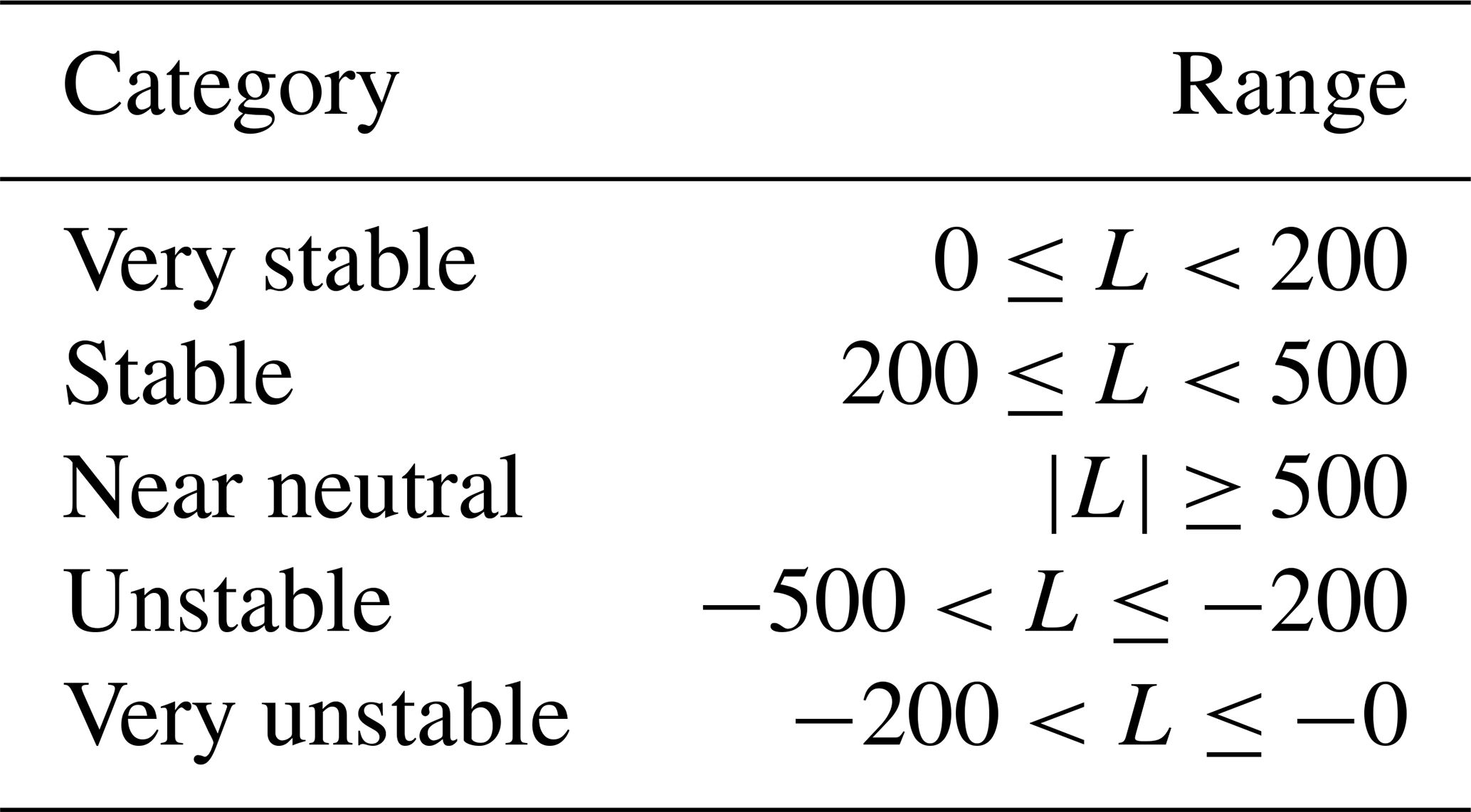
where T_v is the virtual temperature (K) approximated as the air temperature, p₀ is a reference pressure (Pa), p is the pressure at a given height (Pa), and $R/C_{\mathrm{p}}\approx \mathrm{0.286}$. Herein, θ_v was approximated as the air temperature due to a lack of localized pressure and moisture measurements. Further, because not all 47 towers had temperature measurements available at 10 m, the virtual potential temperature for the horizontal homogeneity analysis (described later) was assumed to be a uniform 300 K. The L values were binned according to a schema adapted from Gryning et al. (2007) (Table 2).

Table 2 Obukhov length binning classifications adapted from Gryning et al. (2007).

2.3.3 Turbulence kinetic energy (TKE)

TKE quantifies turbulence in the flow via covariances. The mean TKE, $\stackrel{\mathrm{‾}}{\mathrm{TKE}}$ (m² s⁻²), is calculated as

$$\begin{array}{}\text{(4)}& \stackrel{\mathrm{‾}}{\mathrm{TKE}}={\displaystyle \frac{\mathrm{1}}{\mathrm{2}}}[\stackrel{\mathrm{‾}}{{u^{\prime }}^{\mathrm{2}}}+\stackrel{\mathrm{‾}}{{v^{\prime }}^{\mathrm{2}}}+\stackrel{\mathrm{‾}}{{w^{\prime }}^{\mathrm{2}}}],\end{array}$$

where u^′, v^′, and w^′ (m s⁻¹) are the Reynolds perturbation components from the mean wind (Stull, 1988). In all cases, perturbations are based on a block averaging window over the relevant time period.

2.3.4 Turbulence dissipation rate (ϵ)

The turbulence dissipation rate, ϵ (m² s⁻³), represents the rate at which TKE is dissipated or converted into heat (Stull, 1988) and was calculated using the structure function method (Piper and Lundquist, 2004; Muñoz-Esparza et al., 2018; Wildmann et al., 2019). According to this method, ϵ is related to a second-order structure function, D_U(τ), by the following relation:

$$\begin{array}{}\text{(5)}& \mathit{ϵ}={\displaystyle \frac{\mathrm{1}}{U\mathit{\tau }}}\left[a{D}_U\right(\mathit{\tau }){]}^{\frac{\mathrm{3}}{\mathrm{2}}},\end{array}$$

where U is the horizontal velocity (m s⁻¹), a=0.52 is the Kolmogorov constant, τ is the temporal separation (s), and D_U(τ) is the structure function:

$$\begin{array}{}\text{(6)}& D_U\left(\mathit{\tau }\right)=\langle \left[U\right(t+\mathit{\tau })-U(t){]}^{\mathrm{2}}\rangle ,\end{array}$$

where 〈〉 denotes the ensemble average, and τ was treated as 2 s, consistent with prior analyses (Bodini et al., 2018; Wildmann et al., 2019; Bodini et al., 2019). To calculate ϵ, every 30 s, a centered 2 min window of data was targeted. The structure function was applied to this 2 min window, and the average value of the relevant structure function was retained for each ϵ calculation. These data were maintained at a 30 s resolution because ϵ varies on a shorter timescale than L or TKE and is also not defined by a Reynolds decomposition window.

2.3.5 Reynolds decomposition time

Both L and TKE require Reynolds decomposition calculations (Stull, 1988; Reynolds, 1895). In a Reynolds decomposition, any variable ψ is split into a mean $\stackrel{\mathrm{‾}}{\mathit{\psi }}$ and a turbulent component ψ′. The separation between these two components is determined by the Reynolds decomposition averaging window. Because determining a Reynolds decomposition window that appropriately differentiates mean behavior from turbulent motions is consequential to the resultant stability characterization, many methods to determine the Reynolds decomposition window exist.

Both L and TKE decomposition windows were calculated according to both a 30 min window and a 10 min window based on wind energy industry conventions (IEC, 2022). While we also considered using a variable window based on a multi-flux-resolution decomposition (MRD) approach (Howell and Mahrt, 1997), a previous investigation of the Perdigão dataset with the MRD determined that the MRD was insufficient, so we instead adopted a consistent 30 min averaging approach for this dataset (Mosso et al., 2025).

An appropriate averaging window was determined using an ogive-type method, the cumulative flux averaging–window convergence method (CFAW–CM). While the ogive method (Desjardins et al., 1989; Oncley et al., 1996; Babić et al., 2012) identifies an appropriate Reynolds averaging window through spectral integration of the flux cospectrum in the frequency domain, the convergence method determines the window in the time domain by identifying the averaging period beyond which additional low-frequency variability no longer contributes to the flux covariance. This assessment was performed to determine whether a uniform averaging period could be utilized for heat fluxes ($\stackrel{\mathrm{‾}}{w^{\prime }{\mathit{\theta }}_{\mathrm{v}}^{\prime }}$) and friction velocities ($\stackrel{\mathrm{‾}}{u_{*}}$) across various heights, times of day, and tower locations. By evaluating the cumulative eddy flux contribution according to increasing averaging periods, an asymptote separates local turbulent fluctuations from larger-scale (mesoscale) fluctuations. For this dataset, heat flux and friction velocity values were calculated at each height for each tower location according to 1, 5, 10, 20, 30, and 60 min Reynolds decomposition windows. All values for a given Reynolds decomposition period were then averaged to a single value for that averaging period. To differentiate between times of day, the heat flux values were divided into 00:00–02:00 and 12:00–14:00 UTC to represent nighttime (assumed stable) and daytime (assumed unstable) values, respectively. Based on this analysis, we used a consistent 30 min Reynolds decomposition window for both stable and unstable cases at all towers.

Secondly, we considered the wind energy industry standard, which uses a constant 10 min averaging window (Bailey et al., 1997; IEC, 2022). This standard assumes a clear separation or “spectral gap” (Van der Hoven, 1957) between large-scale mesoscale motions and small-scale turbulence, which does not always exist (Larsén et al., 2013; Kang and Won, 2016; Larsen et al., 2018).

2.4 Post-processing

Extrema were screened out of the stability metric calculations. This screening process involved isolating the distribution of values for each stability metric according to a given Reynolds decomposition window and replacing values outside of a given threshold with not a number (NaN). A common 99.5th percentile threshold was established to simultaneously remove anomalous data and protect representative data. Further, time periods flagged according to one stability metric were not necessarily flagged according to another, ensuring that the representativeness of each stability metric could be evaluated independently.

The process to apply this extrema threshold was tailored to each metric. Obukhov length (L) extrema were flagged by extrema in u_*, $\stackrel{\mathrm{‾}}{w^{\prime }{t}_c^{\prime }}$, and $\stackrel{\mathrm{‾}}{{\mathit{\theta }}_{\mathrm{v}}}$ (Eq. 1). This decision to flag the constituent variables of the Obukhov length as opposed to the Obukhov length itself both ensured consistency across all stages of the calculations and avoided targeted removal of near-neutral cases. Collectively, this Obukhov length screening process removed 1.16 % of L values.

Friction velocity (u_*) extrema were identified as u_* values greater than the 99.5th percentile of the 30 min u_* distribution (1.15 m s⁻¹). The same (i.e., 1.15 m s⁻¹) 30 min u_* threshold was also applied to the 10 min u_* distribution to avoid mischaracterizing larger 10 min u_* values as extrema.

Heat flux $\stackrel{\mathrm{‾}}{w^{\prime }{t}_c^{\prime }}$ extrema were identified according to a process similar to that used to identify extrema in u_*, although the $\stackrel{\mathrm{‾}}{w^{\prime }{t}_c^{\prime }}$ extrema were flagged on both sides of the distribution. The 30 min distribution determined both the 30 and the 10 min threshold for $\stackrel{\mathrm{‾}}{w^{\prime }{t}_c^{\prime }}$, as was the case with u_*. However, in contrast, $\stackrel{\mathrm{‾}}{w^{\prime }{t}_c^{\prime }}$ extrema were identified by flagging the most extreme 0.5th percentile of the positive and negative $\stackrel{\mathrm{‾}}{w^{\prime }{t}_c^{\prime }}$ values separately. This distinction based on the heat flux sign ensured that both stable and unstable cases were screened and that these screenings were independent. This screening identified data greater than 0.582 K m s⁻¹ and less than −0.179 K m s⁻¹. These screening values correspond to 642.5 and −218.0 W m⁻², assuming that the product of the density of moist air, ρ_air, and the specific heat of air, C_p, is 1216 W m⁻² (K m s⁻¹)⁻¹ (Stull, 1988).

Mean virtual potential temperature ($\stackrel{\mathrm{‾}}{{\mathit{\theta }}_{\mathrm{v}}}$) extrema were also flagged on both sides of the distribution, although the underlying data considered for the $\stackrel{\mathrm{‾}}{{\mathit{\theta }}_{\mathrm{v}}}$ process differed from those considered for the u_* and $\stackrel{\mathrm{‾}}{w^{\prime }{t}_c^{\prime }}$ processes. While the u_* and $\stackrel{\mathrm{‾}}{w^{\prime }{t}_c^{\prime }}$ screening processes considered data from all 47 towers, the $\stackrel{\mathrm{‾}}{{\mathit{\theta }}_{\mathrm{v}}}$ screening process only considered temperature measurements from the three 100 m towers to determine a reliable screening threshold. This distinction was made to account for the inconsistent temperature availability across the site. The net result of this $\stackrel{\mathrm{‾}}{{\mathit{\theta }}_{\mathrm{v}}}$ screening was that $\stackrel{\mathrm{‾}}{{\mathit{\theta }}_{\mathrm{v}}}$ values less than 279.97 K or greater than 307.39 K were flagged.

The TKE extrema screening process was most analogous to that employed for u_*. TKE values greater than the 99.5th percentile of the 30 min distribution (4.85 m² s⁻²) were flagged. Because the TKE screening depended only on TKE itself, 0.15 % of TKE values were flagged. Finally, the log ₁₀ϵ extrema screening process removed data from the top (−0.505) and bottom (−5.51) 0.5th percentiles, again constituting 1 % of log ₁₀ϵ values.

2.5 Stability assessment

The variability in atmospheric stability was evaluated with two criteria: the hub-height predictive index (HHPI) and horizontal homogeneity (HoH). These criteria, described more fully below, collectively describe the sensitivity of stability in time, altitude, and spatial location.

Atmospheric stability was first evaluated based on the HHPI. The HHPI assessment was designed to assess how well surface-level classifications predicted classifications at a representative wind turbine hub height of 100 m. This assessment could provide insight into whether surface measurements could predict hub height behavior without the investment of a full 100 m tower. While many representative heights may be potentially considered in a wind farm resource assessment, the hub height is one such representative measurement. Further, the hub height, with typical values near 100 m, aligns with the highest available measurement from the meteorological towers during the Perdigão field campaign. The vertical information propagation over the 100 m tower is also assumed to be much shorter than the Reynolds decomposition window. The L HHPI was calculated as the fraction of cases in which the surface value and the aloft value showed the same stability classification. The TKE and ϵ HHPI were represented by the linear regression R² between the surface and aloft values for each metric. The HHPI assessment was also extended to other intermediate heights present on the towers (i.e., 20, 40, 60, and 80 m). For this extension of the HHPI analysis, the regression or agreement classification was performed by treating each of the intermediate heights as the base height compared to the 100 m hub-height calculations. This HHPI assessment is also performed for a flat-terrain field campaign as a point of comparison in Appendix B.

Each metric was also evaluated for HoH. This assessment was designed to quantify the smallest number and location of meteorological towers necessary to capture the site's variability in surface (10 m) stability. For each metric, all 47 towers with sonic anemometers were considered. Because only 18 of these towers had available 10 m temperature measurements, the virtual potential temperature was assumed to be a uniform 300 K for the Obukhov length calculation just for the HoH analysis. Thus, this analysis could not account for differences in virtual potential temperature that might occur between towers. This approach to addressing the lack of available temperature measurements was determined to be optimal because other potential solutions – such as performing the analysis at either a shorter or a taller height – further limited the number of available towers or relied on data fully within the vegetation layer. Shifting to 20 m would only allow 38 of the 47 towers to be analyzed. Shifting to 30 m would only leave 17 towers. Analyzing 100 m would only leave 3 data points. These other solutions also devalued the assessment as a practical demonstration of how stakeholders could leverage surface-level measurements to inform site characterization. These 47 towers were then represented as a graph network, with a node for each tower location and the edge weights representing the strength of similarity in surface stability between any two given towers. This similarity metric, S, mapped the correlation in surface stability, C_ij, with only positive edge weights such that $S=\frac{(C_{ij}+\mathrm{1})}{\mathrm{2}}$. The smallest number of meteorological towers was then determined based on the Louvain community detection algorithm (Blondel et al., 2008), as implemented by the NetworkX Python package (Hagberg et al., 2008). Note that the Louvain algorithm, unlike kNN methods, treats the number of clusters as an output instead of an input. It determines which towers are redundant by identifying tower subgroups and assigning each tower to one of these subgroups. It also enforces (non)treatment of overlapping communities, further ensuring that each community is treated independently with a unique tower. While the Louvain community detection algorithm is also sensitive to several tuning parameters, we make no adjustments to the default modularity gain threshold ($\mathrm{1}\times {\mathrm{10}}^{-\mathrm{7}}$) or resolution (1), introduce no artificial seeds, and do not establish restrictions on the number of optimization cycles.

Another optimization was then employed on the available partitions to determine a potential optimal tower layout. This optimization, performed with the pulp Python library (Mitchell et al., 2011), treats the available partitions as a standard Hitting set (Karp, 1972) problem. As such, all available partitions across metrics and averaging periods were analyzed to determine the minimum number of towers necessary to span the full partition set. This tower set, represented graphically with stars, is non-unique. Thus, while other layouts could be considered equally viable, the starred tower set represents one possible layout that requires the smallest number of towers.

The Louvain community detection algorithm was also applied separately to large-eddy simulation (LES) from Robey and Lundquist (2024). This analysis serves as a proof-of-concept implementation to demonstrate how this methodology can extend to model output. Both the methodology and the results of this analysis are provided in Appendix C.

3 Results

3.1 Site characterization

3.1.1 Radiation analysis

Before proceeding with stability analysis, we ensured that influences like topographic shading of our measurements did not directly impact parts of our analysis. In particular, we ensured that our designated “stable” and “unstable” hours did not experience inequitable solar exposure between towers. Importantly, these designations also translated to our CFAW–CM convergence analysis, which informed the Reynolds decomposition window.

All three 100 m towers likely experience shading during some part of the day. The incoming shortwave solar radiation near all towers shows a typical diurnal cycle for a mid-latitude land-based site (Fig. 3). This diurnal cycle is defined by low (i.e., zero) incoming shortwave radiation in the late (18:00–24:00 UTC) and early morning (00:00–04:00 UTC) hours, with an increase throughout the morning (05:00–11:00 UTC), a midday peak (12:00–14:00 UTC), and a late afternoon drop (15:00–17:00 UTC) (Fig. 3). Within this diurnal cycle, differences in solar exposure throughout the day emerge. These differences in solar exposure contribute to differences in residuals. While negligible positive residuals may reflect measurement uncertainties, negative residuals are assumed to reflect shading.

Both the morning (05:00–07:00 UTC) and the early evening (15:00–17:00 UTC) experience shading (Fig. 3). Cloudy days (Fig. 3a, c, e) naturally exhibit more shading than cloudless days (Fig. 3b, d, f) near each of the three 100 m towers. This diurnal difference in shading is especially pronounced in the valley, where negligible shading is suggested during cloudless days (Fig. 3d). Non-cloud-based shading due to diurnal differences in solar exposure also influences the two 100 m ridge towers. While shading in the valley is only imposed by clouds (Fig. 3c, d), the two ridges show stronger terrain-induced shading (Fig. 3a, b, e, f). Further, while the SW ridge experiences minimal terrain-induced shading in the early evening (Fig. 3b), the NE ridge shows the strongest terrain-induced shading during both the early morning and the early evening (Fig. 3f). Local canopy effects may then contribute – but not define – non-cloud shading. The NE ridge shows more diurnal shading than the SW ridge and also has a taller canopy cover. However, the valley has canopy cover but experiences no non-cloud shading. Further, the SW ridge, with a negligible canopy cover, does experience non-cloud shading. Thus, shading from the larger ridge topography may also contribute to diurnal shading. Regardless of the exact shading source, these site-based differences in shading suggest that sites do not have equivalent diurnal exposure to the incoming solar radiation. Our CFAW–CM analysis, described below, accounts for these differences in solar exposure by only considering cloudless days and restricting the stable and unstable periods to 00:00–02:00 and 12:00–14:00 UTC, respectively.

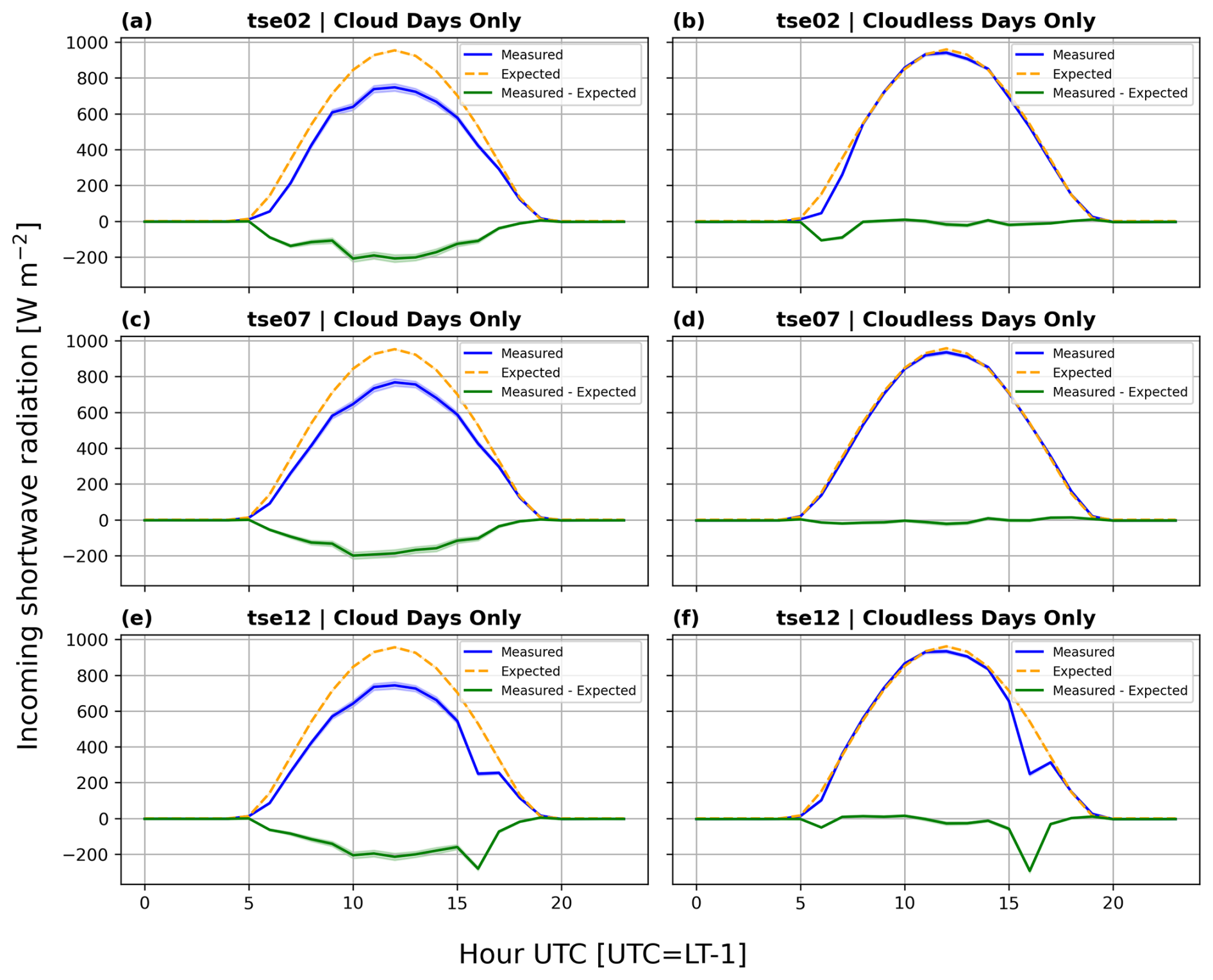
Figure 3 Comparison between expected and measured incoming shortwave radiation adjacent to each of the three 100 m towers. The line represents the mean value, and the band represents the standard error. (a) tse02 (SW ridge) cloud days only, (b) tse02 (valley) cloudless days only, (c) tse07 (NE ridge) cloud days only, (d) tse07 (SW ridge) cloudless days only, (e) tse12 (valley) cloud days only, and (f) tse12 cloudless days only.

3.1.2 Cumulative flux averaging–window convergence method (CFAW–CM) analysis

We recommend a uniform 30 min Reynolds decomposition window based on the results from the CFAW–CM analysis. Most heights, sites, and metrics support this analysis, with a few exceptions.

The CFAW–CM assessment, as described above, seeks to identify the Reynolds decomposition time that is long enough to incorporate all contributions by turbulence without including larger mesoscale contributions. This window is determined by identifying the asymptote before an increase assumed to be associated with mesoscale motions. For example, for heat flux in the valley (Fig. 4d, e, f), values increase as the averaging time grows from 1 to 10 min but stay constant between 10 and 30 min and increase at 60 min, thereby suggesting that an averaging period between 10 and 30 min is justifiable.

A 30 min Reynolds decomposition period is consistently supported by valley observations. Friction velocities (Fig. 5d) increase sharply from 1–5 min, level from 5–30 min, and then sharply increase again at 60 min, indicating that 30 min captures turbulence fluctuations. This conclusion applies regardless of stability. Under stable conditions, valley heat fluxes (Fig. 4e) remain small and nearly insensitive to an averaging period longer than 5 min, while friction velocities (Fig. 5e) plateau between 20–30 min, before increasing at 60 min, again supporting a 30 min window. During unstable conditions, heat fluxes (Fig. 4f) level off after 10 min and increase again between 30–60 min, whereas friction velocities (Fig. 5f) stabilize at 5 min before increasing again after 30 min. Together, these metrics confirm that a 30 min Reynolds decomposition period is appropriate in the valley, regardless of the stability condition.

A 30 min Reynolds decomposition period is also appropriate for most conditions on the two ridges. Under unstable stratification, both heat fluxes (Fig. 4c, i) and friction velocities (Fig. 5c, i) consistently support a 30 min window. Heat fluxes (Fig. 4c,i) increase from 1–20 min before leveling off, while friction velocities show similar behavior. On the SW ridge, unstable friction velocities (Fig. 5c) – especially above 10 m – stabilize by 10 min, whereas on the NE ridge, they increase until about 20 min at heights above 20 m and remain constant from 1–30 min at heights at or below 20 m (Fig. 5i). Together, these patterns justify a 30 min decomposition period for unstable conditions on both ridges.

During stable conditions, the suitability of a 30 min window differs between the ridges. On the NE ridge, heat fluxes (Fig. 4h) are mostly constant throughout 30 min before increasing from 30–60 min. Although friction velocities at 100 m continue to increase beyond 60 min, those at all other heights (Fig. 5h) behave more cleanly: they increase slightly from 1–20 min, plateau between 20–30 min, and then increase again between 30–60 min (Fig. 5h). Thus, a 30 min Reynolds decomposition period remains viable on the NE ridge, across metrics and stability conditions.

In contrast, stable conditions on the SW ridge are less well-represented by a 30 min window. Heat fluxes at 10–40 m continue to increase beyond 60 min, although those fluxes at 60–100 m are nearly constant from 1–30 min before jumping between 30–60 min (Fig. 4b). Stable friction velocities on the SW ridge increase steadily beyond 60 min at all heights, suggesting a need for a longer Reynolds decomposition window (Fig. 5b).

The CFAW–CM analysis also highlights the contrasts between ridge and valley sites. Heat fluxes are larger and friction velocities are smaller on the ridges compared to those in the valley (Figs. 4 and 5). Valley heat fluxes (Fig. 4d) exhibit tighter spread than those on either ridge (Fig. 4a, g). Valley friction velocities (Fig. 5d) increase with height, whereas ridge friction velocities (Fig. 5a, g) decrease with altitude, with the exception of unstable friction velocities on the NE ridge (Fig. 5i), which resemble the valley (Fig. 5f). These site-based differences motivate further analysis in the following section.

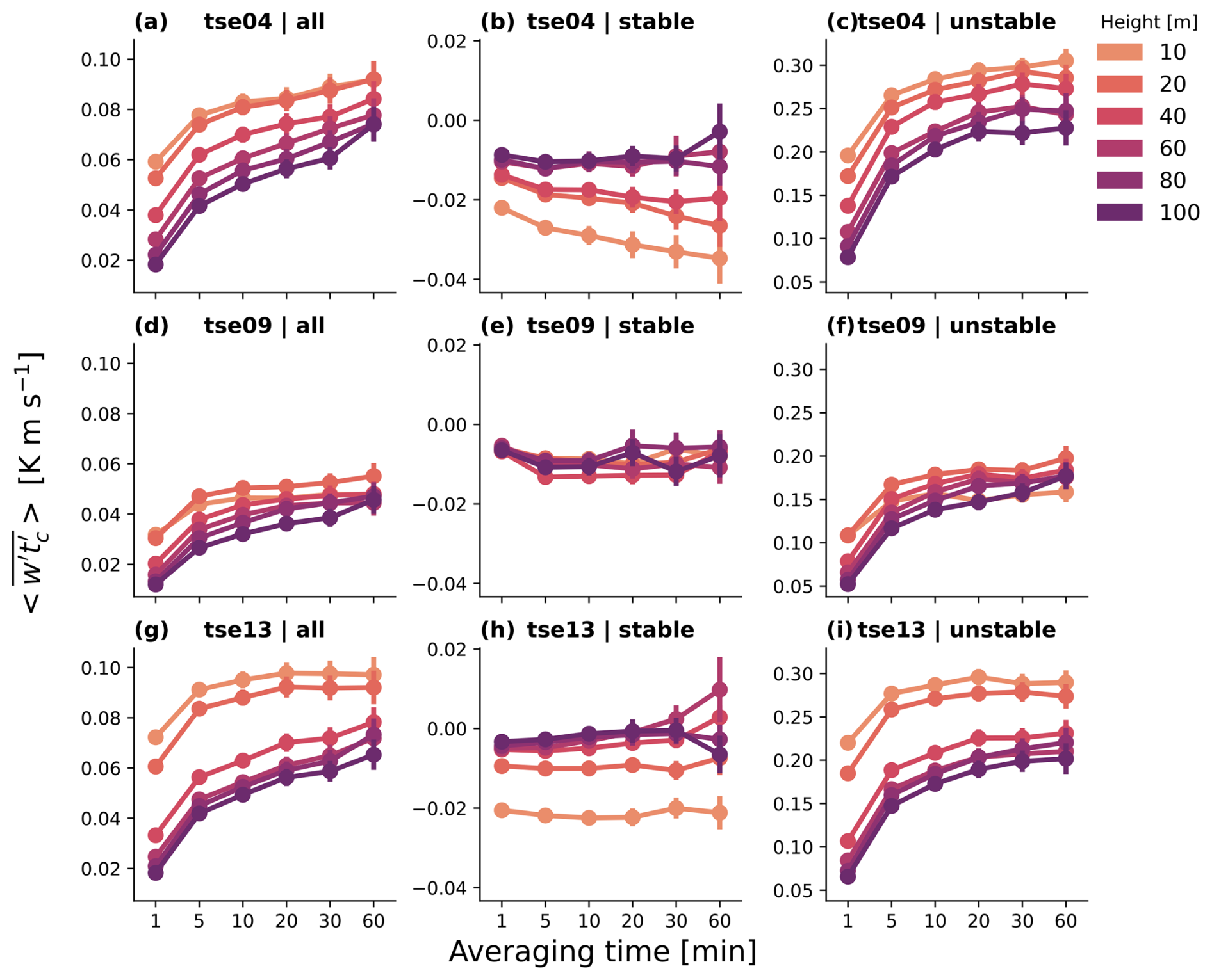
Figure 4 CFAW–CM analysis of heat fluxes at each 100 m tower (tse04 (SW ridge): a, b, c; tse09 (valley): d, e, f; tse13 (NE ridge): g, h, i) and each available height, for all (a, d, g), stable (00:00–02:00 UTC, b, e, h), and unstable (12:00–14:00 UTC, c, f, i) cases. The points represent the mean value for a tower–height combination, and the error bars represent the standard error. (a) tse04 overall (SW ridge), (b) tse04 (SW ridge) stable, (c) tse04 (SW ridge) unstable, (d) tse09 (valley) overall, (e) tse09 (valley) stable, (f) tse09 (valley) unstable, (g) tse13 (NE ridge) overall, (h) tse13 (NE ridge) stable, and (i) tse13 (NE ridge) unstable.

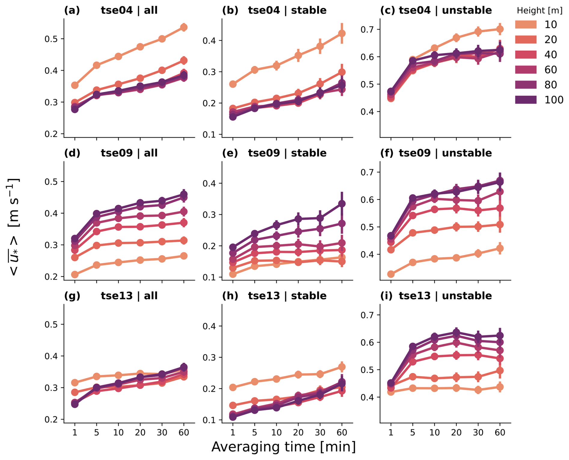
Figure 5 CFAW–CM analysis of u_* at each 100 m tower (tse04 (SW ridge): a, b, c; tse09 (valley): d, e, f; tse13 (NE ridge): g, h, i) and each available height, for all (a, d, g), stable (00:00–02:00 UTC, b, e, h), and unstable (12:00–14:00 UTC, c, f, i) cases, as in Fig. 4. The points represent the mean value for a tower–height combination, and the error bars are described with the standard error.

3.1.3 Vertical profiles

Ridges and valleys reflect distinct profiles. Heat fluxes are larger on the two ridges than in the valley (Fig. 6d). This distinction in heat flux magnitude is especially clear during unstable conditions (Fig. 6f), where the mean surface heat flux on the SW ridge is twice that in the valley. The unstable heat flux profile in the valley also reflects a sharp increase from 10 to 20 m that is not reflected for the two ridges (Fig. 6f). Instead, those along the two ridges decrease from the surface (Fig. 6f).

Stable heat flux profiles also reflect profoundly distinct shapes between the ridges and the valley (Fig. 6e). Stable heat flux profiles along the two ridges are more stable than in the valley at the surface, but as the height increases, the stable heat fluxes along the two ridges become increasingly weaker (Fig. 6e). In contrast, the stable heat flux profile in the valley (Fig. 6e) becomes more stable from the surface to 40 m before stabilizing above. Thus, while the valley is well-mixed during stable conditions, the ridges are not (Fig. 6e). This unique heat flux behavior in the valley during stable conditions is also corroborated by the heat flux CFAW–CM analysis, where stable heat fluxes in the valley (Fig. 4e) are much tighter and smaller than those along the two ridges (Fig. 4b, h). These ridge–valley differences in stable heat fluxes may signal an upside-down boundary layer in the valley (Fig. 6e).

Ridge and valley distinctions are also reflected in the friction velocity profiles. Friction velocities begin larger at the surface along the two ridges and decrease before leveling between 20–40 m (Fig. 6a). In contrast, valley friction velocities are smaller at the surface and increase aloft, eventually overtaking the friction velocities along the two ridges (Fig. 6a). These profile shapes are further reinforced for friction velocities during stable conditions (Fig. 6b).

Friction velocities during unstable conditions subvert these ridge and valley distinctions. Here, friction velocities on the NE ridge reflect those in the valley both in magnitude and in shape, increasing from a small surface value (Fig. 6c). In this case, only the SW ridge opposes the valley by demonstrating a ridge-like friction velocity profile (Fig. 6c).

Both flow and terrain features may contribute to this NE ridge subversion. Menke et al. (2019) documented recirculation zones during over half of the unstable periods. These flows could then explain why this unique behavior is reflected only during unstable cases. Menke et al. (2019) also documented that these recirculation flows occurred more frequently near the valley and NE ridge than near the SW ridge. Thus, recirculation zones provide a mechanism that is aligned in terms of geography and stability condition to explain this behavior. Canopy effects may also contribute to this NE ridge subversion. The NE ridge is, like the valley, covered with vegetation with a canopy (Table 1, Fig. 2c) that increases the surface roughness. In contrast, the SW ridge, which is more exposed (Table 1, Fig. 2a), may not have this potential. Quimbayo-Duarte et al. (2022), Venkatraman et al. (2023), and Al Oqaily et al. (2025) have also all documented that increasing the surface roughness layer characterizations improves wind speed model performance for this region. Thus, the enhanced drag from the canopy may be reinforced by recirculation flows occurring during unstable conditions.

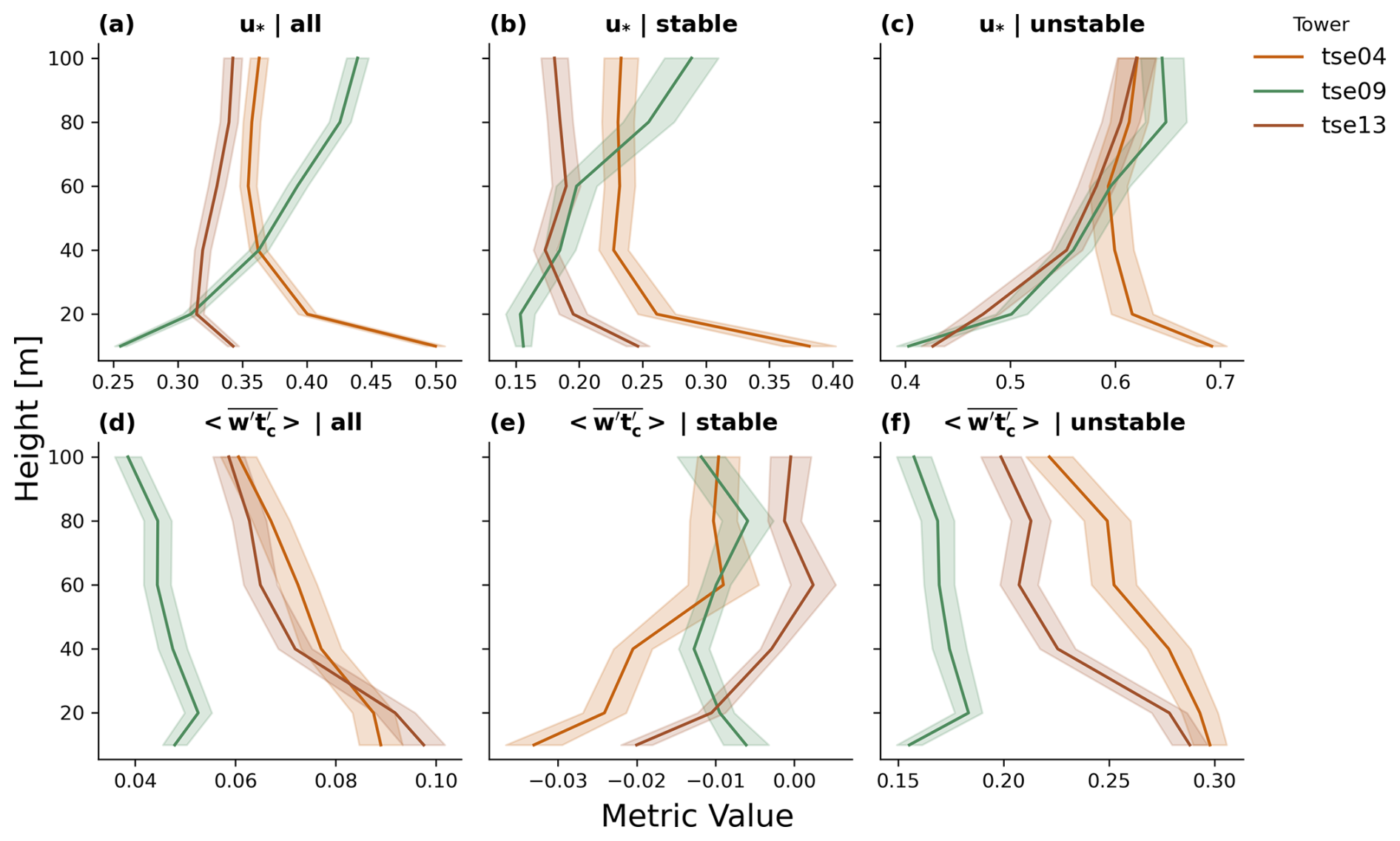
Figure 6 Perdigão field campaign vertical profiles with 30 min averaging at the three 100 m towers. The solid line indicates the mean value, and the band represents the standard error. (a) Friction velocity all (00:00–23:00 UTC), (b) friction velocity stable (00:00–02:00 UTC), (c) friction velocity unstable (12:00–14:00 UTC), (d) heat flux all (00:00–23:00 UTC), (e) heat flux stable (00:00–02:00 UTC), and (f) heat flux unstable (12:00–14:00 UTC).

3.1.4 Wind roses and their spatial and vertical variability

Ridge and valley distinctions are also reinforced in winds. The 30 min wind roses for the three 100 m towers differ between the valley (Fig. 7c and d) and the ridges (Fig. 7a, b, e, and f). Both the SW (Fig. 7a) and the NE (Fig. 7e) ridge surface winds show primarily a northeasterly flow. In contrast, the surface valley winds (Fig. 7c) show primarily a southeasterly flow. Further, the surface valley winds (Fig. 7c) are slower than the surface winds on either of the two ridges (Fig. 7a and e). The wind roses for the three 100 m towers also differ between the 10 m surface winds and the 100 m winds. The 100 m winds at all three tower locations (Fig. 7b, d, and f) are less bidirectional than the winds at their respective 10 m locations. The 100 m winds at all three tower locations are also generally faster and more consistent than the winds at their respective 10 m locations. These site and height distinctions between wind roses are also preserved, regardless of the averaging window (not shown).

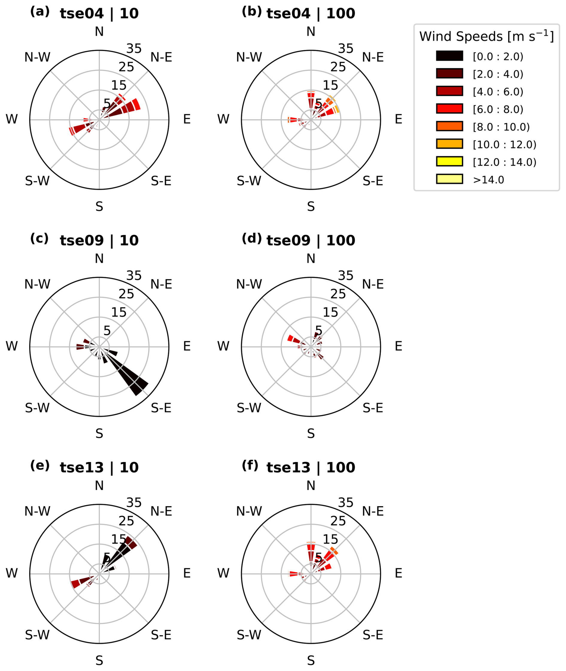
Figure 7 Perdigão (cloud-removed) field campaign wind rose with 30 min averaging at the three 100 m towers and at 10 m (a, c, e) and 100 m (b, d, f) altitudes. The rings (i.e., 5, 15, 25, 35) correspond to the percentage of data that aligns with a given speed and direction. (a) tse04 (SW ridge) at 10 m, (b) tse04 (SW ridge) at 100 m, (c) tse09 (valley) at 10 m, (d) tse09 (valley) at 100 m, (e) tse13 (NE ridge) at 10 m, and (f) tse13 (NE ridge) at 100 m.

3.1.5 Diurnal variability

All three stability metrics exhibit a strong diurnal cycle (Figs. 8–15) that would be expected for this onshore mid-latitude region in late spring/early summer.

The L diurnal cycle (Fig. 8) differs between the ridges (Fig. 8a, b, e, f) and the valley (Fig. 8c, d). The general L diurnal cycle shows mostly stable (S) and very stable (VS) cases in the early morning (00:00–05:00 UTC) and evening (21:00–00:00 UTC) hours, with a shift toward mostly unstable (U) and very unstable (VU) cases in the middle of the day (06:00–20:00 UTC) at all locations (Fig. 8). The valley L diurnal cycle is unique in its larger relative percentage of near-neutral cases aloft (Fig. 8d). Further, the L diurnal cycles on the two ridges have negligible near-neutral cases aloft (Fig. 8b). The L diurnal cycle in the valley is also unique in its reduction in the relative contribution of VU cases from the surface (Fig. 8c) to aloft (Fig. 8d). Again, while the L diurnal cycle on the NE ridge has more VU cases at the surface (Fig. 8e) than aloft (Fig. 8f) throughout all daytime hours, the L diurnal cycle on the SW ridge shows more similar frequencies of VU cases between the surface (Fig. 8a) and aloft (Fig. 8b) in the morning, with fewer VU cases at 100 m in the later afternoon. Of note, the SW ridge has a smaller percentage of VU cases than either the valley or the NE ridge.

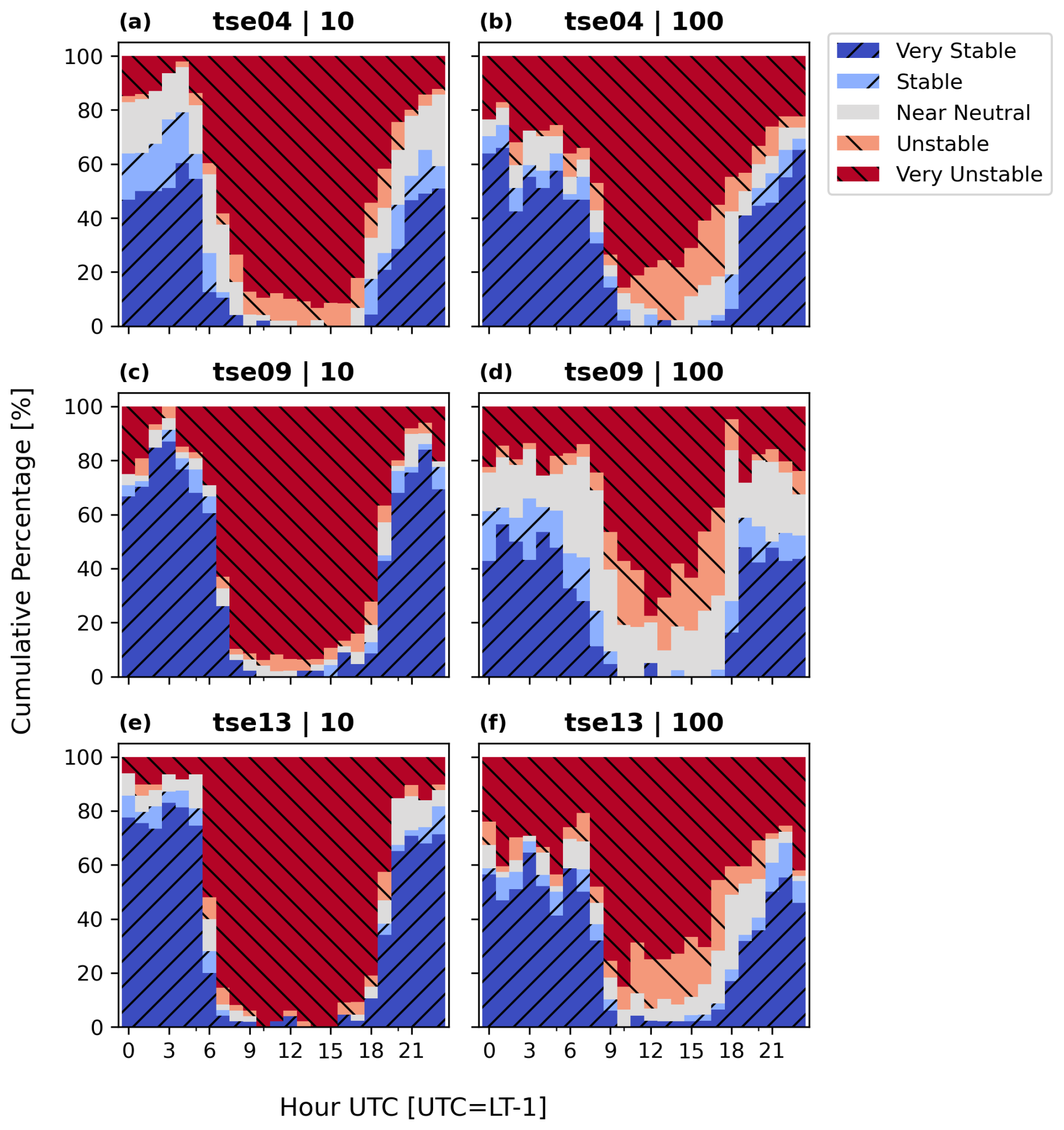
Figure 8 L diurnal cycle for (cloud-removed) campaign period with 30 min averaging: (a) tse04 (SW ridge) at 10 m, (b) tse04 (SW ridge) at 100 m, (c) tse09 (valley) at 10 m, (d) tse09 (valley) at 100 m, (e) tse13 (NE ridge) at 10 m, and (f) tse13 (NE ridge) at 100 m.

The u_* diurnal cycle (Fig. 9) can explain the site-based differences in the reduction in VU contribution. u_* shows smaller values in the early morning (00:00–05:00 UTC) and evening (19:00–00:00 UTC) hours, with a shift toward larger values in the middle of the day (06:00–20:00 UTC) at all heights. The middle-of-day u_* in the valley also increases from 10 m measurements (Fig. 9c) to measurements at 100 m (Fig. 9d), suggesting an increased role of mechanical forcing and therefore a decreased role of buoyant forcing. This shift corresponds to a reduction in the representation of VU cases from the surface (Fig. 9c) to aloft (Fig. 9d). A similar trend exists at the NE ridge. Again, the middle-of-day u_* increase from the surface (Fig. 9e) to aloft (Fig. 9f) corresponds to a reduced contribution from VU cases. In contrast, the middle-of-day u_* at the SW ridge does not increase from the surface (Fig. 9a) to aloft (Fig. 9b) but actually decreases slightly. This middle-of-day u_* decrease from the surface to aloft along the SW ridge suggests a reduced role of mechanical forcing and therefore an increased role of buoyant forcing, thereby supporting the consistent number of VU cases between the surface and aloft at the SW ridge in the morning hours (09:00–12:00 UTC).

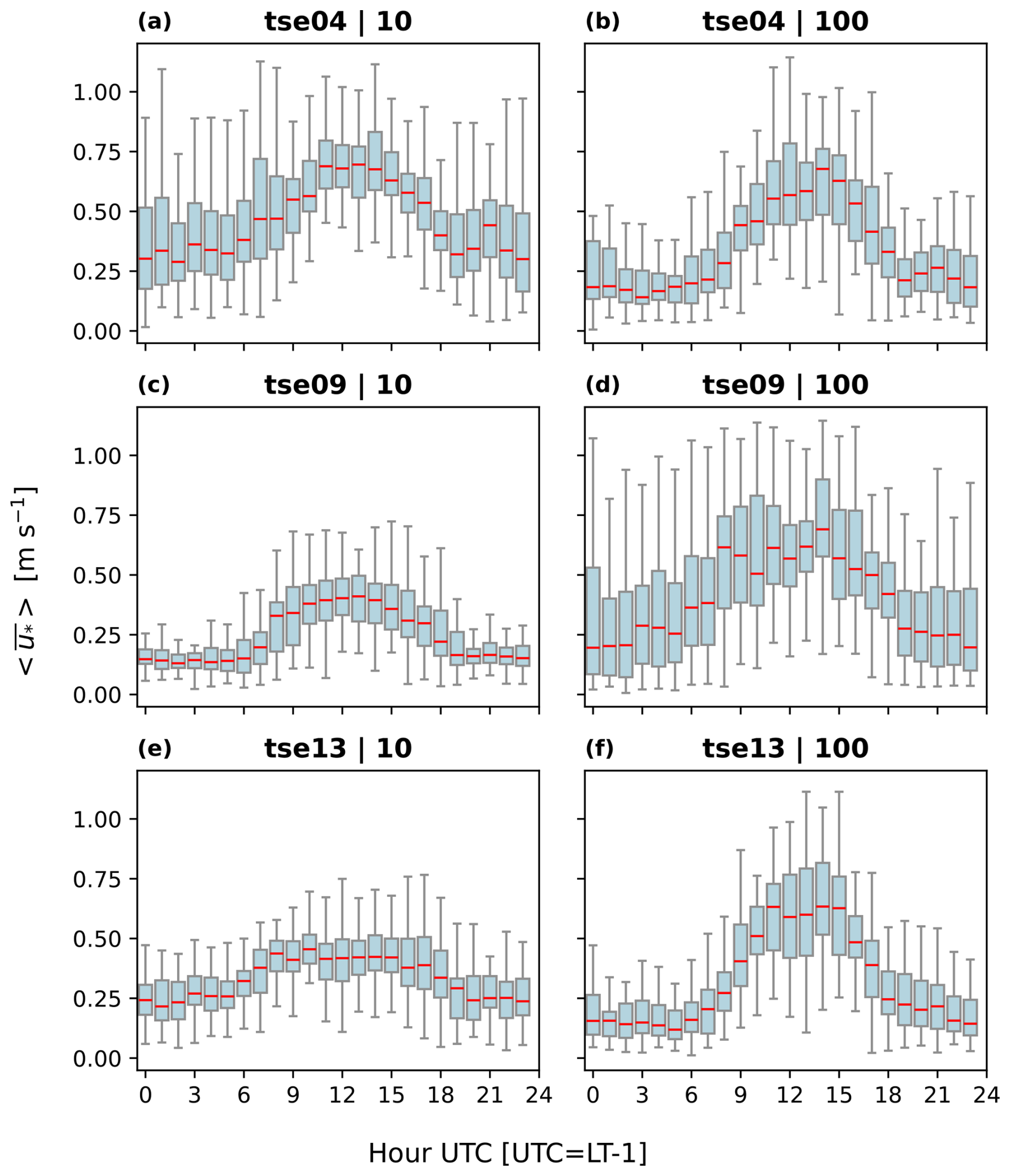
Figure 9 u_* diurnal cycle for (cloud-removed) campaign period. The red lines indicate the median, and the box and whiskers are defined based on Q1 (25th percentile), Q3 (75th percentile), and the interquartile range (IQR) (Q3–Q1). The box encloses the IQR, and the whiskers extend to $\mathrm{Q}\mathrm{1}-\mathrm{1.5}\cdot \mathrm{IQR}$ and $\mathrm{Q}\mathrm{3}+\mathrm{1.5}\cdot \mathrm{IQR}$. (a) tse04 (SW ridge) at 10 m, (b) tse04 (SW ridge) at 100 m, (c) tse09 (valley) at 10 m, (d) tse09 (valley) at 100 m, (e) tse13 (NE ridge) at 10 m, and (f) tse13 (NE ridge) at 100 m.

In contrast, the heat flux ($\stackrel{\mathrm{‾}}{w^{\prime }{t}_c^{\prime }}$) diurnal cycle (Fig. 10) cannot explain the reduced VU contribution aloft in the valley. The heat flux is smaller in the early morning (00:00–05:00 UTC) and evening (19:00–00:00 UTC) hours and grows in the middle of the day (06:00–20:00 UTC). The midday maximum in heat flux along the two ridges is larger at the surface (Fig. 10a and e) than aloft (Fig. 10b and f). Further, in the valley, the midday heat flux maximum grows from the surface (Fig. 10c) to aloft (Fig. 10d).

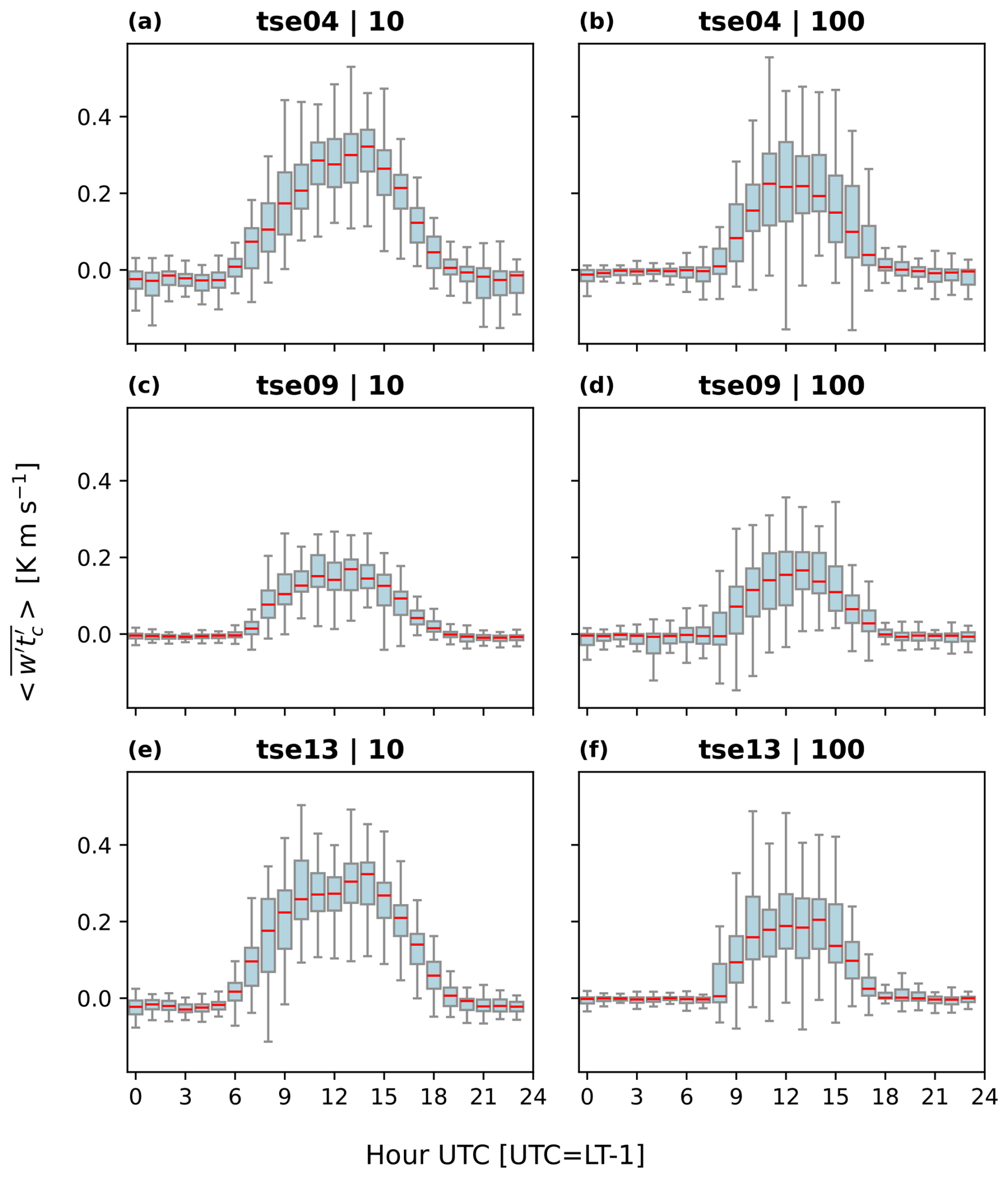
Figure 10 Heat flux diurnal cycle for (cloud-removed) campaign period with 30 min averaging. The red lines indicate the median, and the box and whiskers are defined based on Q1 (25th percentile), Q3 (75th percentile), and the interquartile range (IQR) (Q3–Q1). The box encloses the IQR, and the whiskers extend to $\mathrm{Q}\mathrm{1}-\mathrm{1.5}\cdot \mathrm{IQR}$ and $\mathrm{Q}\mathrm{3}+\mathrm{1.5}\cdot \mathrm{IQR}$. (a) tse04 (SW ridge) at 10 m, (b) tse04 (SW ridge) at 100 m, (c) tse09 (valley) at 10 m, (d) tse09 (valley) at 100 m, (e) tse13 (NE ridge) at 10 m, and (f) tse13 (NE ridge) at 100 m.

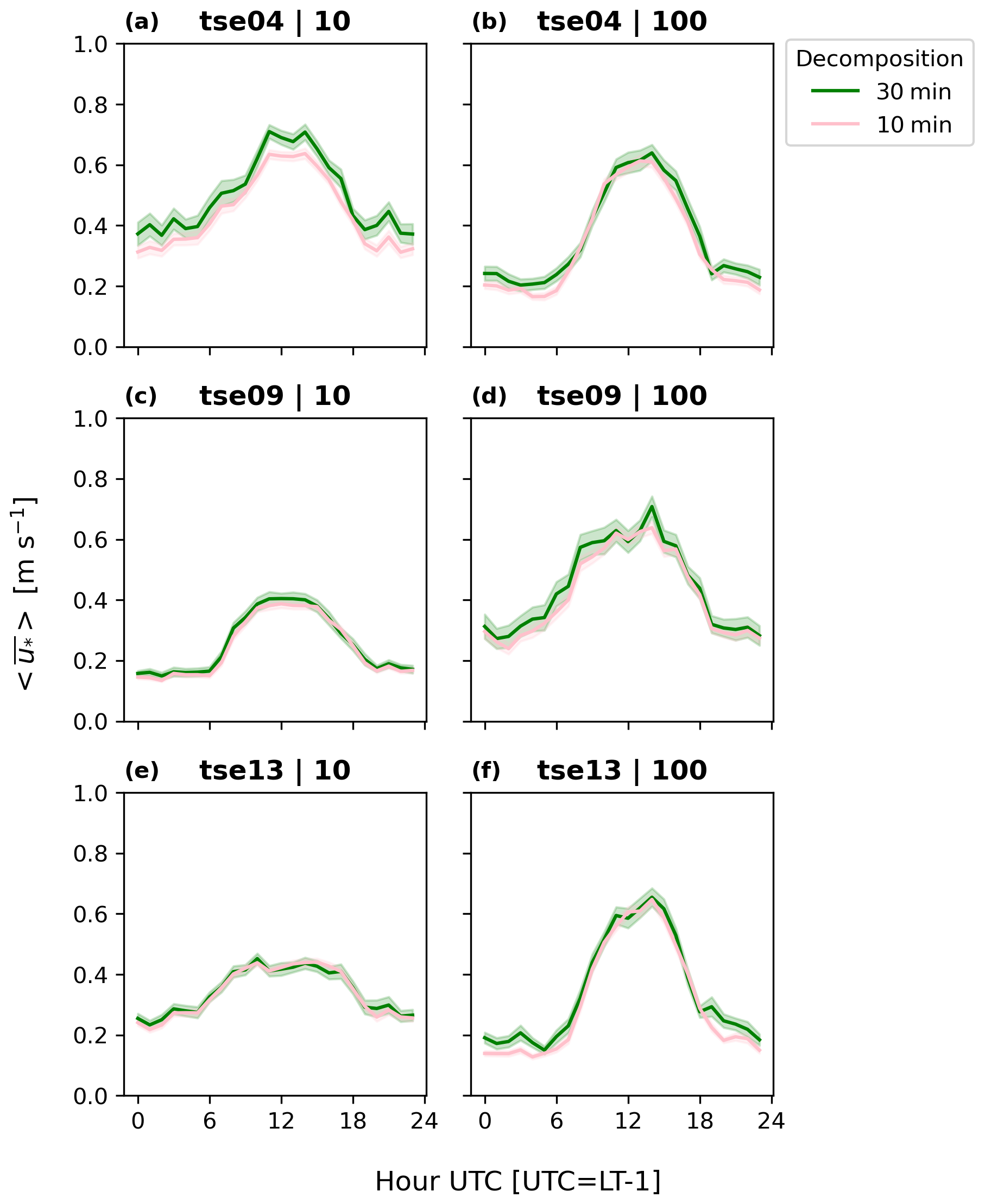
Figure 11 u_* diurnal cycle for (cloud-removed) campaign period according to two decomposition intervals. The solid line indicates the mean value, and the band indicates the standard error. (a) tse04 (SW ridge) at 10 m, (b) tse04 (SW ridge) at 100 m, (c) tse09 (valley) at 10 m, (d) tse09 (valley) at 100 m, (e) tse13 (NE ridge) at 10 m, and (f) tse13 (NE ridge) at 100 m.

Further, the u_* diurnal cycle appears regardless of the decomposition period. u_* is the smallest during the morning hours (00:00–05:00 UTC), peaks in the middle of the day (06:00–20:00 UTC), and then drops again in the evening (21:00–24:00 UTC), regardless of the Reynolds decomposition period. During unstably stratified periods, u_* according to the 10 min Reynolds decomposition period is smaller than u_* based on a 30 min Reynolds decomposition period. This inability of the 10 min Reynolds decomposition period to resolve the full flux is most apparent at 10 m on the SW ridge (Fig. 11a).

The maximum u_* values found in the stable periods of the u_* diurnal cycle also vary between the Reynolds decomposition periods. During these stable periods, the 30 min averaging approach yields the highest u_*, followed by the 10 min averaging approach. Again, this discrepancy at the surface is the largest on the SW ridge (Fig. 11a). In contrast, the valley aloft (Fig. 11d) shows larger u_* differences based on the Reynolds decomposition period during stable periods than the two ridges (Fig. 11b, f).

The TKE diurnal cycle is also smaller in the early morning (00:00–05:00 UTC) and evening (21:00–00:00 UTC) hours and grows in the middle of the day (06:00–20:00 UTC) (Fig. 12). While all three tower locations show larger values aloft (Fig. 12b, d, and f) than at the surface (Fig. 12a, c, and e), this trend is especially pronounced in the valley (Fig. 12b and c), perhaps due to advection of surface-generated turbulence from the ridges. Further, the valley shows a more muted diurnal cycle at 10 m (Fig. 12c) than the ridges (Fig. 12a and e).

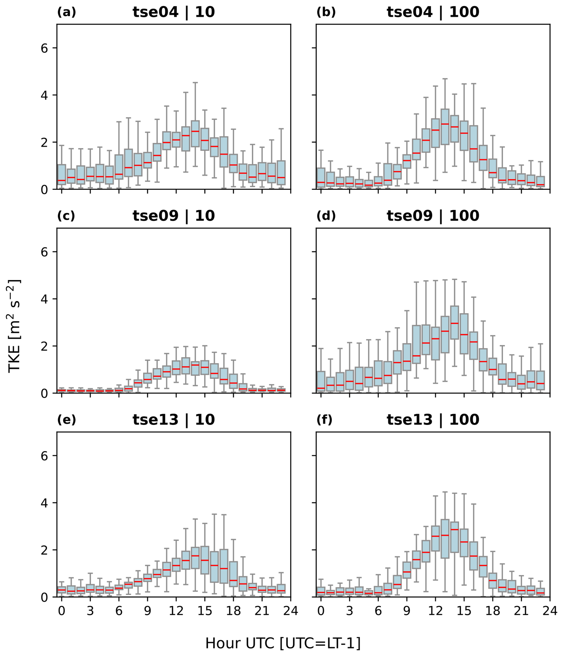
Figure 12 TKE diurnal cycle for (cloud-removed) campaign period with 30 min averaging. The red lines indicate the median, and the box and whiskers are defined based on Q1 (25th percentile), Q3 (75th percentile), and the interquartile range (IQR) (Q3–Q1). The box encloses the IQR, and the whiskers extend to $\mathrm{Q}\mathrm{1}-\mathrm{1.5}\cdot \mathrm{IQR}$ and $\mathrm{Q}\mathrm{3}+\mathrm{1.5}\cdot \mathrm{IQR}$. (a) tse04 (SW ridge) at 10 m, (b) tse04 (SW ridge) at 100 m, (c) tse09 (valley) at 10 m, (d) tse09 (valley) at 100 m, (e) tse13 (NE ridge) at 10 m, and (f) tse13 (NE ridge) at 100 m.

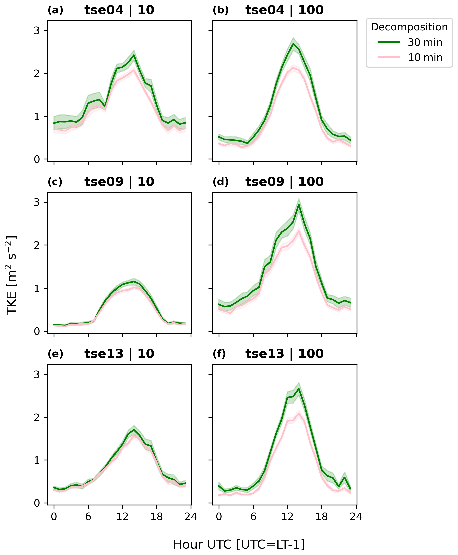
Figure 13 TKE diurnal cycle at three towers (tse04: a, b; tse09: c, d; tse13: e, f) for the (cloud-removed) campaign period according to two averaging approaches at two heights (10 m: a, c, e; 100 m: b, d, f). The solid lines indicate the mean value, and the bands indicate the standard error. (a) tse04 (SW ridge) at 10 m, (b) tse04 (SW ridge) at 100 m, (c) tse09 (valley) at 10 m, (d) tse09 (valley) at 100 m, (e) tse13 (NE ridge) at 10 m, and (f) tse13 (NE ridge) at 100 m.

The TKE diurnal cycle also emerges regardless of the decomposition approach, with a maximum value of TKE that is sensitive to the averaging period used. TKE is smaller during the early morning and evening hours and grows in the middle of the day for all Reynolds decomposition windows, as was the case with u_* (Fig. 13) and as expected over land. Also consistent with the behavior observed with the u_* diurnal cycle, during stably stratified periods, 30 min TKE and 10 min TKE are smaller (Fig. 13). This stable-period discrepancy based on the Reynolds decomposition window is pronounced at the surface only on the SW ridge (Fig. 13a) but for all locations aloft (Fig. 13b, d, f). At the same time, the TKE diurnal cycle (Fig. 13) varies more during unstable periods based on the Reynolds decomposition window than the u_* diurnal cycle (Fig. 11). This spread based on the Reynolds decomposition window observed in the TKE emerges at both altitudes for all three towers (Fig. 13).

These trends in the TKE diurnal cycle also occur at intermediate heights (Fig. 14), with the largest differences at 10 m in the valley and on the canopied NE ridge. The TKE in the valley (Fig. 14c, d) shows stratified layers during nighttime hours, with smaller values at the surface and larger values with increasing height.

One way to explain this apparent decoupling in the valley between the 10 m and 100 m measurements is to consider remote generation of turbulence that is then advected to the upper levels of the valley tower. This advection could occur horizontally such that turbulence generated on the ridge is advected into the valley, where it is dissipated. This process could also occur vertically through the presence of an upside-down boundary layer (Parker and Raman, 1993; Mahrt, 1999). Warm air on the ridges may be advected over cold air pooled and trapped in the valley, leading to shear generation at the top of the cold pool (Mahrt, 1999). The explanation of an upside-down boundary layer in the valley is supported by a consistent TKE increase across intermediate heights between 10 and 100 m within the valley (Fig. 14c, d) but not at the two ridge locations (Fig. 14a, b, e, f). This unique, well-mixed behavior during stable conditions in the valley is also reflected in the heat fluxes (Fig. 6e).

During the daytime period, the valley site shows stratification as well. This TKE stratification in the valley also persists for both Reynolds decomposition approaches. The 30 min valley TKE (Fig. 14c) differs most strongly between 10 and 100 m, especially during the unstable middle of the day (Fig. 14d). The 10 min valley TKE (Fig. 14e) reduces the peak TKE and the gap between 10 and 100 m TKE. The TKE on the NE ridge (Fig. 14e, f) reflects some of the same stratification as the valley (Fig. 14c, d), although the stratification on the NE ridge is less extreme. Further, while the upper-level TKE diurnal cycles are similar, the 10 m TKE remains separate on the NE ridge (Fig. 14e, f), similar to what is observed in the valley (Fig. 14c, d). The TKE diurnal decoupling on the NE ridge is unique, however, in that the 10 m TKE pattern at this location increases at 18:00 UTC during the early evening transition, while the 10 m TKE in the valley continues its decrease. The TKE diurnal cycle on the SW ridge (Fig. 14a, b) does not stratify into layers, regardless of the Reynolds decomposition window.

Canopy effects may help explain this 10 m TKE decoupling during unstable conditions in the valley and NE ridge. These 10 m measurements, located within the canopy layer but not necessarily within the vegetation layer, could experience heightened turbulence that would necessarily be reflected at taller measurements. Recirculation zones, also present during unstable conditions in the valley and NE ridge, may also influence this TKE decoupling. However, as noted in Menke et al. (2019), the depth of these recirculation zones exceeds 100 m. Thus, because these recirculation zones would not necessarily impact 10 m measurements uniquely, their effect may be secondary to the more direct influence of the canopy.

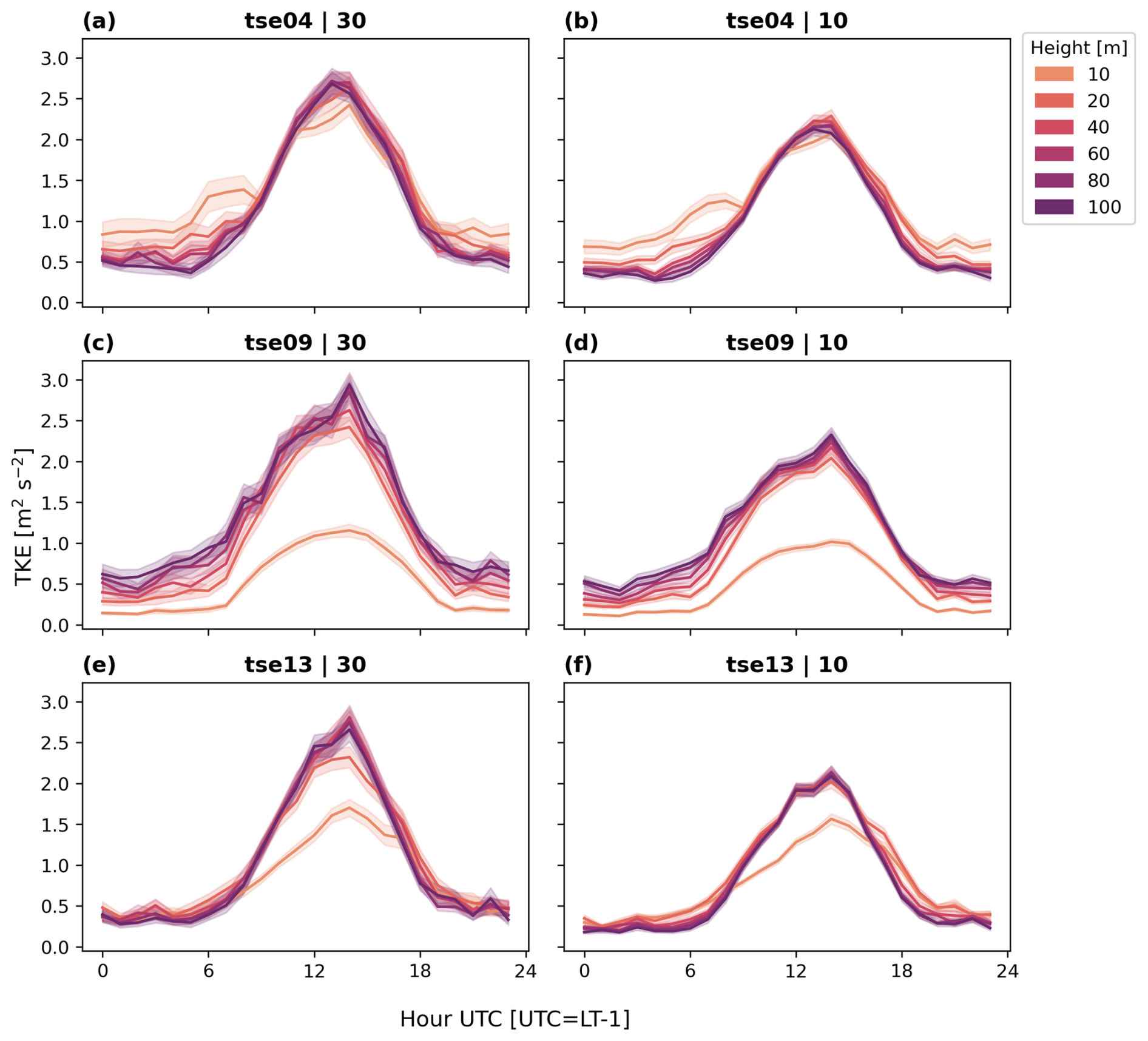
Figure 14 Diurnal cycle of TKE at all heights for each 100 m tower (tse04: a and b; tse09: c and d; tse13: g and h) according to two averaging approaches (30 min: a, c, e; 10 min: b, d, f). The solid line indicates the mean value, and the band is the standard error. (a) tse04 (SW ridge) 30 min, (b) tse04 (SW ridge) 10 min, (c) tse09 (valley) 30 min, (d) tse09 (valley) 10 min, (e) tse13 (NE ridge) 30 min, and (f) tse13 (NE ridge) 10 min.

The ϵ diurnal cycle is the least pronounced of the three metrics considered (Fig. 15), which has implications for numerical modeling of flow in this complex terrain. While generally smaller values occur in the morning (00:00–05:00 UTC) and evening (21:00–00:00 UTC) hours and larger values in the middle of the day (06:00–20:00 UTC), the diurnal cycle is muted both at the surface on the NE ridge (Fig. 15e) and aloft in the valley (Fig. 15d). The ϵ diurnal cycle also differs between the ridges (Fig. 15a, b, e, and f) and the valley (Fig. 15c and d). While the two ridges show smaller ϵ values aloft (Fig. 15b and f) than at the surface (Fig. 15a and e) (opposite of the TKE trends), the valley shows relatively consistent ϵ values between the surface (Fig. 15c) and aloft (Fig. 15d). The valley's larger values may again be due to advection of turbulence from the neighboring ridges, which must then dissipate in the valley. This local imbalance of dissipation rate, as seen also in Wildmann et al. (2019), has implications for numerical models that assume local balance between production and dissipation.

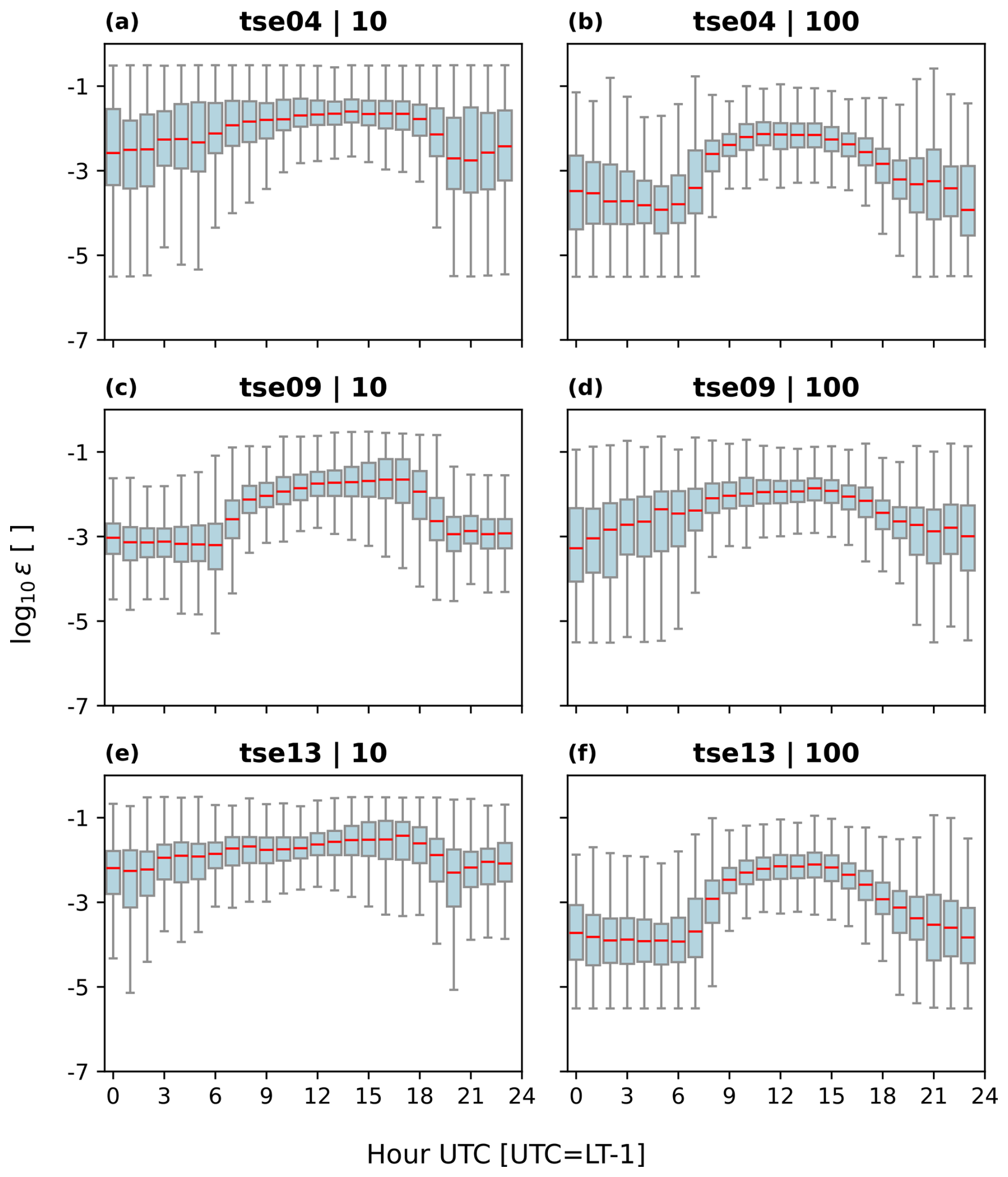
Figure 15 ϵ diurnal cycle for (cloud-removed) campaign period. The red lines indicate the median, and the box and whiskers are defined based on Q1 (25th percentile), Q3 (75th percentile), and the IQR (Q3–Q1). The box encloses the IQR, and the whiskers extend to $\mathrm{Q}\mathrm{1}-\mathrm{1.5}\cdot \mathrm{IQR}$ and $\mathrm{Q}\mathrm{3}+\mathrm{1.5}\cdot \mathrm{IQR}$. (a) tse04 (SW ridge) at 10 m, (b) tse04 (SW ridge) at 100 m, (c) tse09 (valley) at 10 m, (d) tse09 (valley) at 100 m, (e) tse13 (NE ridge) at 10 m, and (f) tse13 (NE ridge) at 100 m.

3.2 Stability metric analysis

3.2.1 Hub-height predictive index

Perdigão surface (10 m) measurements fail to represent conditions at turbine hub height (100 m). The surface L rate of agreement is 50 % or lower for all three towers (Fig. 16). For TKE, surface HHPI is quantified by correlation and shows poor and comparable R² for all tower locations. The SW ridge has a smaller TKE surface HHPI (Fig. 16). The ϵ surface HHPI also shows very poor performance (Fig. 16), with R² values always less than 0.3, and especially poor performance on the NE ridge. This consistently poor surface HHPI leaves ϵ as the worst metric to make hub-height predictions based on surface measurements.

Measurements at higher altitudes lead to larger HHPI for all metrics (Fig. 16). The overall L HHPI profile shows negligible variability based on tower. Each tower begins with an L HHPI of approximately 0.4–0.5 and steadily increases to an L HHPI of approximately 0.6–0.7, regardless of the tower location (Fig. 16a, b, c). The TKE HHPI profile consistently shows larger HHPI than the other two metrics overall, regardless of the location (Fig. 16a, b, c). Further, while the TKE HHPI increase is consistent within the valley (Fig. 16b), this increase is more discontinuous along the two ridges (Fig. 16a, c). The ϵ HHPI profile shows the largest increase across heights and the greatest consistency across tower locations. Although the ϵ HHPI (Fig. 16) at the surface is the lowest of the three metrics, the ϵ HHPI (Fig. 16) steadily increases to (slightly) overtake the L HHPI (Fig. 16) at all three sites (Fig. 16a, b, c).

The valley is the site with HHPI most impacted by the Reynolds decomposition window. All three sites experience HHPI improvements with a longer averaging window, corroborating the role of the enhanced TKE characterization. However, these performance improvements are negligible along the two ridges (Fig. 17a, b, g, h). In contrast, the TKE HHPI in the valley maintains an approximately 0.1 improvement at low altitudes with the longer window (Fig. 17b). This performance improvement with a longer window in the valley further corroborates the already-noted TKE stratification in the valley (Fig. 14c, d).

The otherwise consistent performance between the 10 and 30 min Reynolds decomposition windows does not necessarily suggest that 10 min Reynolds decomposition windows and 30 min Reynolds decomposition windows resolve similar fluxes. In fact, several analyses in this work, including CFAW–CM (Figs. 4 and 5) and diurnal cycles (Figs. 8–15), suggest otherwise. Rather, because the HHPI assessment compares stability metrics with the same Reynolds decomposition window, the relative lack of performance improvement with a 30 min Reynolds decomposition window may instead suggest that a longer Reynolds decomposition window may not be an appropriate alternative to building taller towers.

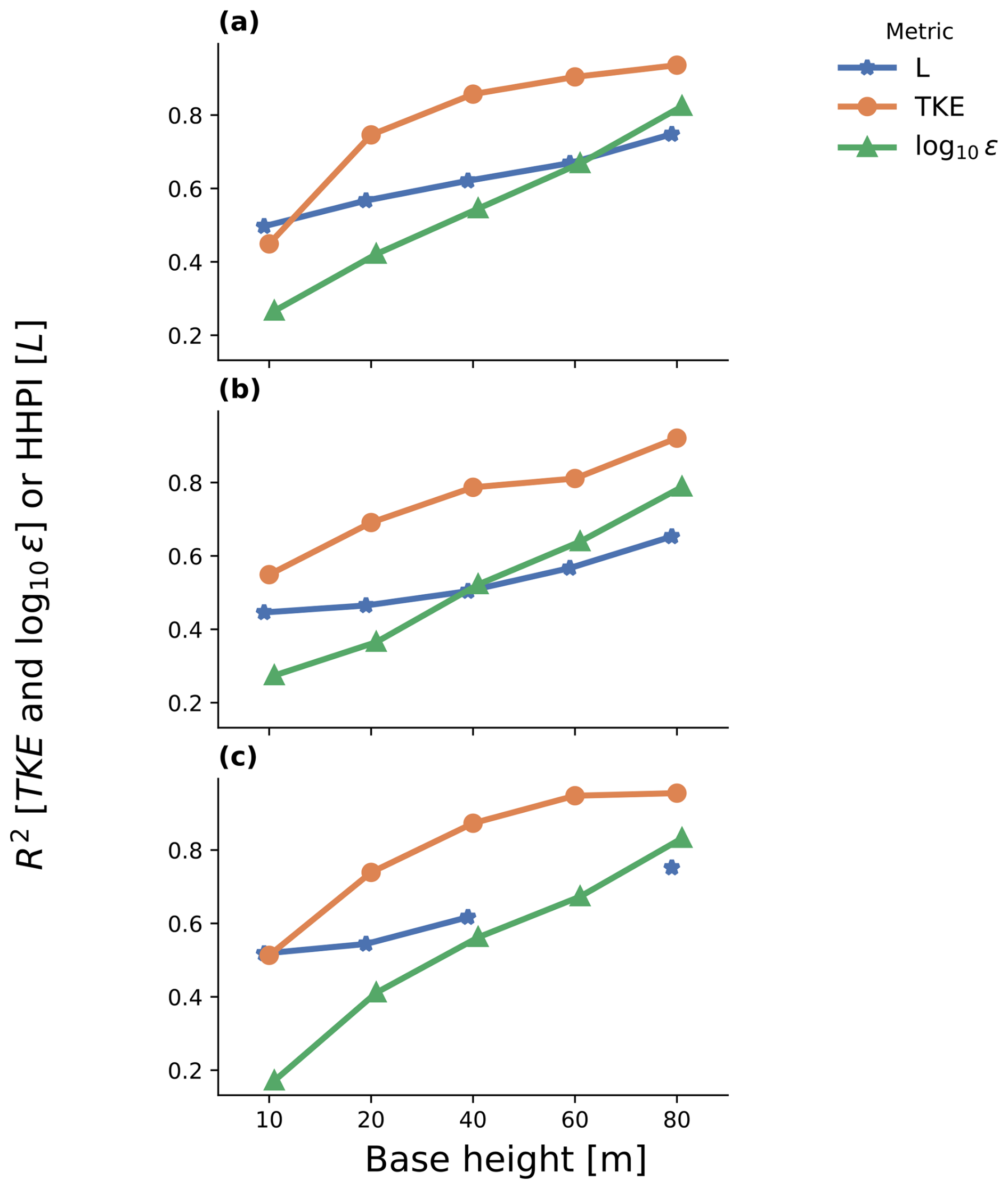
Figure 16 Correlation coefficient between the base height and 100 m for (cloud-removed) campaign period with 30 min averaging. tse13 60 m L calculations were omitted due to high (76 %) temperature data unavailability. (a) tse04 (SW ridge), (b) tse09 (valley), and (c) tse13 (NE ridge).

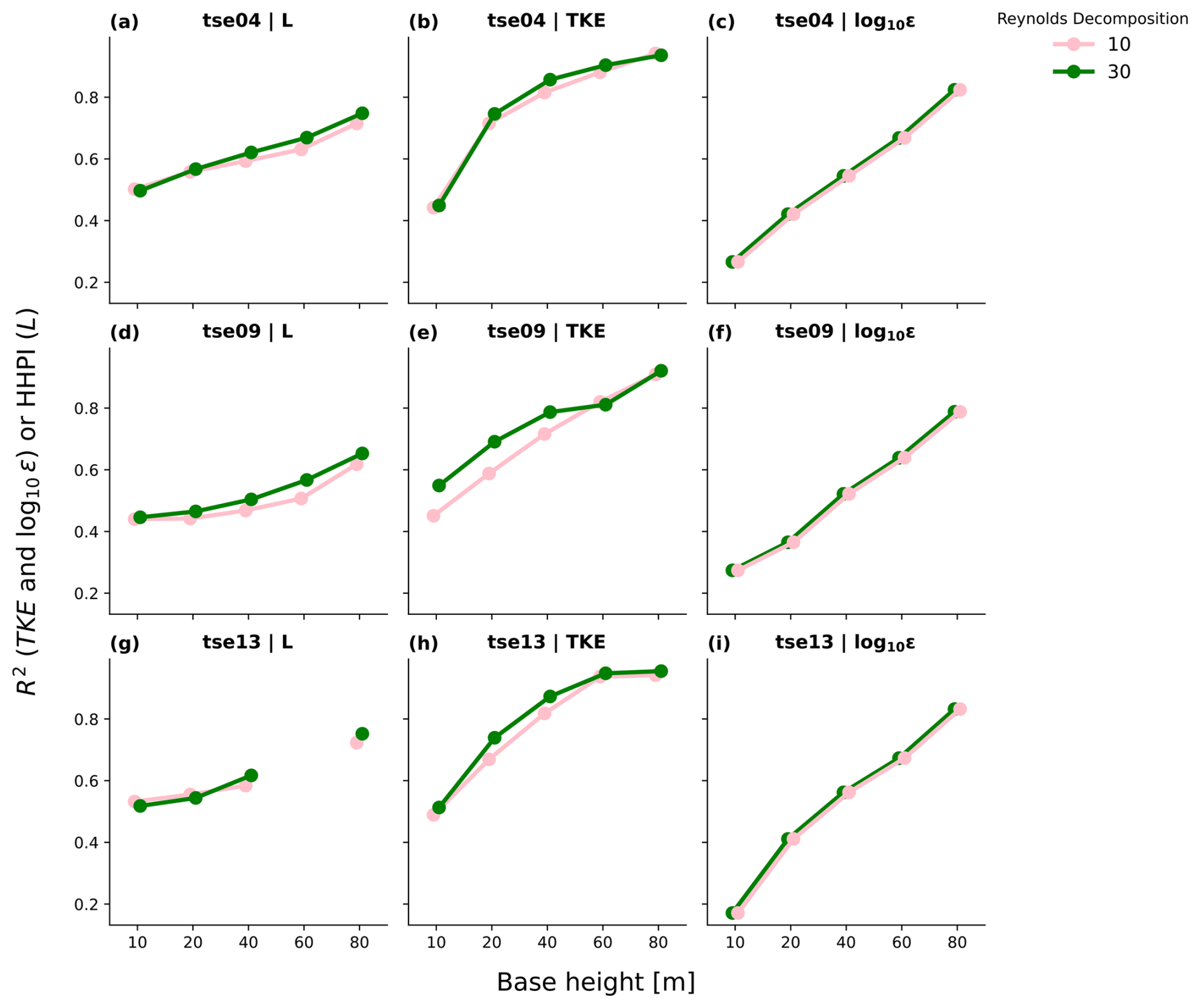
Figure 17 Correlation coefficient between the base height and 100 m for (cloud-removed) campaign period according to two averaging approaches. In all cases, ϵ calculations are maintained at their 30 s resolution. (a) tse04 (SW ridge) L, (b) tse04 (SW ridge) TKE, (c) tse04 (SW ridge) ϵ, (d) tse09 (valley) L, (e) tse09 (valley) TKE, (f) tse09 (valley) ϵ, (g) tse13 (NE ridge) L, (h) tse13 (NE ridge) TKE, and (i) tse13 (NE ridge) ϵ.

3.2.2 Horizontal homogeneity

We sought to define the minimum number of towers to represent the variability in the 10 m measurements at Perdigão using the Louvain community detection algorithm. A nine-tower subset spans all groupings across all metrics (Fig. 18). While this subset is not the only potential subset that spans all groupings across all metrics, this tower subset indicates the smallest number of towers necessary to fully characterize the site's partitions in TKE, L, and ϵ for either Reynolds decomposition window considered here.

The towers cluster into groups that generally follow terrain boundaries. For example, with a 30 min averaging period, the L groupings define a SW ridge (orange) and NE ridge (blue) as well as dark blue and yellow transects. These dark blue and yellow transects are also separated by a valley that is defined by both blue and lavender pockets (Fig. 18a). Similar partitions are also reflected in the TKE and ϵ groupings (Fig. 18c, e).

The TKE and ϵ groupings also differ from those presented with L. Both TKE and ϵ present a more mixed transect as opposed to a single transect (Fig. 18c, e). TKE and ϵ groupings also see the NW transect as distinct from the SE transect (Fig. 18c, e). ϵ groupings are also notably the least able to differentiate between the two ridges themselves (Fig. 18e). The ϵ groupings also suggest a fairly uniform valley (Fig. 18e), while both TKE (Fig. 18c) and L (Fig. 18a) suggest greater variability within the valley.

The Reynolds decomposition window also shifts partitions. Both tnw08 and tse08 shift for both L and TKE between 30 and 10 min. tnw08 shifts from dark blue to turquoise as a distinct partition for both metrics. tse08 also shifts based on the averaging window. For TKE, tse08 is seen as a SW ridge (orange) tower with a 30 min averaging window but as an independent (grey) tower with a 10 min Reynolds decomposition. Clearly, tse08 represents a divide within the valley.

We also see cases where the Reynolds decomposition window shifts the partition for one metric but not another. rne02 shifts an L partition from (relatively unique) pink to being misattributed as a SW ridge tower with a 10 min averaging window. Similarly, tnw04 is determined to be part of the SW transect (dark blue) for 30 min TKE and is more appropriately absorbed with 10 min as mid-blue. This sensitivity in the valley to the Reynolds decomposition window, especially for TKE, is consistent with many results presented in this work (Figs. 14c, d; 17d, e; and 13c, d).

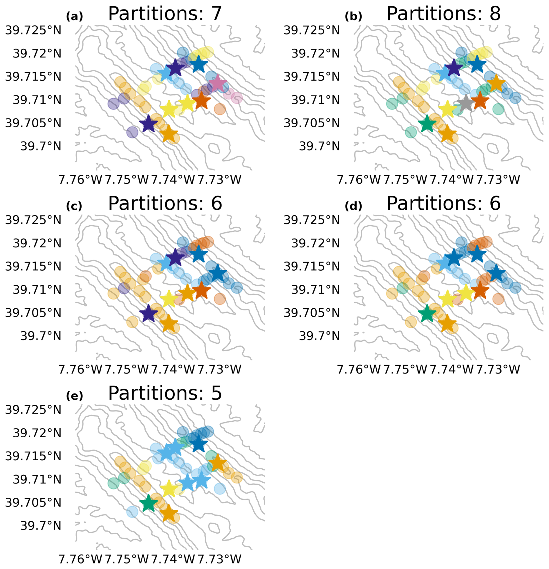
Figure 18 Groupings determined by the Louvain community detection algorithm for each metric. The number of colors corresponds to the number of tower groupings, and towers of the same color correspond to the same tower grouping. A nine-tower subset indicated with stars spans all groupings across all metrics. (a) L 30 min, (b) L 10 min, (c) TKE 30 min, (d) TKE 10 min, and (e) ϵ 30 s.

4 Discussion

Stability metrics are sensitive to the Reynolds decomposition window used to calculate them. Wind energy industry approaches have historically relied on a consistent 10 min averaging period, regardless of the stability regime (IEC, 2022; Bailey et al., 1997; Goit et al., 2022). This 10 min Reynolds decomposition window assumes (and potentially misassumes) clear separation between large-scale mesoscale motions and small-scale turbulent motions and that the 10 min Reynolds decomposition window appropriately distinguishes both regimes. In contrast, a longer, 30 min Reynolds decomposition window has the potential to resolve more turbulent fluctuations while still avoiding larger-scale mesoscale motions. This difference is clearly seen in the maximum TKE values during the middle of the day (Figs. 13, 14), where the 30 min window can include the turbulent circulations that span the deeper daytime convective boundary layer.

The Reynolds decomposition window impacts turbulence characterization on the SW ridge. Notably, 10 m TKE differences between Reynolds decomposition windows are larger on the SW ridge (Fig. 13a) than in the valley (Fig. 13c) or on the NE ridge (Fig. 13e), both during stable and unstable periods. The same is true for the u_* diurnal cycle (Fig. 11). Similarly, the u_* CFAW–CM analysis on the SW ridge reflects anomalous behavior during unstable periods in which a 30 min averaging period is not sufficiently long (Fig. 5).

The Reynolds decomposition window also impacts stability characterization in the valley. The L and TKE partitions in the valley shift depending on whether a 30 min (Fig. 18a) or 10 min Reynolds decomposition window is used during stable periods (Fig. 18b, c). Similarly, the strength of TKE stratification is also influenced by the Reynolds decomposition window (Fig. 14). This more complete characterization of the TKE stratification in the valley with a 30 min Reynolds decomposition window over a 10 min Reynolds decomposition window also translates to an improved TKE HHPI in the valley. Thus, employing the CFAW–CM to determine an optimal (potentially longer) averaging window can improve atmospheric stability characterization.

Increasing the length of the Reynolds decomposition window, however, does not necessarily improve the HHPI for any metrics or locations outside of TKE in the valley. This general lack of HHPI improvements with a longer Reynolds decomposition window does not necessarily suggest that the fluxes are the same. Rather, a longer Reynolds decomposition window may not be a suitable alternative to building taller towers.

The overall small surface HHPI values have potential implications for the utility of shorter towers when information at 100 m is needed. The small HHPI values (Fig. 16) suggest that surface measurements are unable to make hub-height predictions, regardless of the Reynolds decomposition window. Thus, meteorologists may not be able to avoid investing in hub-height-tall meteorological towers to make informed hub-height predictions.

The HoH results also have potential implications for those who need information over a broad area in complex terrain. Results from the Louvain community detection algorithm analysis of the observations suggest shared behavior among towers in common terrain (Fig. 18). Thus, complex-terrain meteorologists may be able to reduce the number of towers necessary to understand surface stability by strategically placing tower locations in areas of differing terrain. Researchers and developers may also consider implementing the Louvain community detection algorithm with flow models such as large-eddy simulations, like those in Wagner et al. (2019), Wise et al. (2022), Robey and Lundquist (2024), and Giani and Crippa (2024) (among others), to assess locations required for tower siting. Appendix C includes a proof-of-concept application of the Louvain community detection algorithm to a short-duration large-eddy simulation.

5 Conclusions

Characterizing atmospheric stability is crucial for multiple wind energy applications and becomes more challenging in heterogeneous, complex terrain. This work demonstrates the challenges in atmospheric stability characterization in complex terrain by analyzing how atmospheric stability varies in the Perdigão valley. We assess the utility of building taller towers at three strategic locations and also consider the optimal tower number and placement to sample variability in the atmospheric stability for the complex site. We perform these assessments based on three stability metrics: the Obukhov length (L), the turbulence kinetic energy (TKE), and the turbulence dissipation rate (ϵ). We also repeat these assessments according to different Reynolds decomposition windows, considering a consistent 30 min averaging window common in the atmospheric science community and a consistent 10 min averaging that is standard in the wind energy community.

Results provide potentially valuable insights for those interested in analyzing areas of complex terrain. For example, 10 m surface measurements do not provide reliable 100 m hub-height stability predictions. Thus, it may be necessary to invest in meteorological towers that extend to hub height to make effective hub-height predictions.

Results here also provide insights regarding approaches to defining the number and location of meteorological towers necessary to accurately characterize a complex-terrain site, at least in terms of atmospheric stability parameters such as TKE, ϵ, and L. Different results occur from variations in wind speed, wind direction, and/or turbulence intensity. Specifically, this analysis suggests that it may be possible to reduce the number of necessary meteorological towers by strategically sampling towers in regions of differing terrain and by coupling community detection algorithms with flow models like those in Wise et al. (2022), Robey and Lundquist (2024), and Giani and Crippa (2024), among others.

Results also reflect how atmospheric stability characterizations are influenced by choices in the Reynolds decomposition window. The Reynolds decomposition window influences stability characterization in the valley, such that a 30 min Reynolds decomposition window during unstable periods better captures maximum values, and during stable periods it clarifies the TKE stratification in this location. Collectively, the results presented herein speak to the challenges that meteorologists and other analysts may face in balancing the need for accurate characterizations of atmospheric stability in areas of complex terrain with the financial implications of investing in meteorological towers.

These results also suggest opportunities for future work that could inform improved characterization of atmospheric stability in complex terrain. Future work could involve extending the assessments presented in this analysis to other sites with complex terrain and with more stability metrics. For example, analyzing heavily vegetated sites and sites over water could improve our understanding of surface roughness length variability and the corresponding similarity relationships. Further, introducing more stability metrics could support evaluations of the relative value of investing in more sensors to calculate the Obukhov length as opposed to more cost-effective stability characterizations (Cantero et al., 2022).

Appendix A

Table A1 Dates included (i.e., not flagged according to the Supplement to Fernando et al., 2019, as presenting low clouds, middle clouds, thunderstorms, or fog) in the analysis.

Appendix B

Here we provide a flat-terrain comparison to the Perdigão HHPI analysis. This flat-terrain benchmark serves to contextualize the role of complex terrain in affecting the relative agreement between surface and hub-height stability. Sonic anemometer data from the Boulder Atmospheric Observatory (BAO) tower during the 3-month eXperimental Planetary boundary layer Instrumentation Assessment (XPIA) (Lundquist et al., 2017; Bodini et al., 2018) field campaign provide the data source for this comparison. Available measurements include data from 5, 50, and 100 m. As such, we compare both 5–100 m and 50–100 m. Each stability metric calculation employs a screening process similar to that employed for the Perdigão data, including removal of approximately 20 % of data affected by precipitation, 99.5th percentile extrema, and tower wake distortion screening.

HHPI is higher in flat terrain than in complex terrain at shorter heights. HHPI in flat terrain is similar to HHPI in complex terrain in several ways. Both improve with taller towers. In both cases, log ₁₀ϵ has the lowest HHPI of all metrics, and this metric distinction is especially pronounced for shorter heights (Fig. B1c). Both terrains also exhibit similar curvatures for each metric. L HHPI is consistently flatter at lower heights and increases more sharply at higher heights (Fig. B1a). TKE HHPI increases more sharply for shorter heights before increasing more gradually above (Fig. B1b). log ₁₀ϵ HHPI is unique in its consistent linear increase (Fig. B1). HHPI in the two terrains also differ. Notably, HHPI is higher in flat terrain than in complex terrain (Fig. B1). Surface L HHPI is between 0.1 and 0.2 higher in flat terrain than in complex terrain (Fig. B1a). Surface TKE HHPI in flat terrain exceeds that in complex terrain by sometimes as much as 0.3 (Fig. B1b). Surface log ₁₀ϵ demonstrates the smallest flat-terrain lead (Fig. B1c). These flat-terrain leads, pronounced at the surface, are not guaranteed at higher heights. While L HHPI continues to reflect a flat-terrain premium (Fig. B1a), both TKE HHPI (Fig. B1b) and log ₁₀ϵ HHPI (Fig. B1c) do not. Thus, while shorter towers may be more useful in flat terrain than in complex terrain, flat-terrain towers may also benefit less from height increases.

Figure B1 Flat-terrain (XPIA) benchmark to the Perdigão HHPI analysis. (a) L, (b) TKE, and (c) log ₁₀ϵ.

Appendix C

Here we demonstrate a proof-of-concept implementation of the Louvain methodology applied to large-eddy simulation (LES) data. This Louvain implementation considers near-surface static stability from the LES of Robey and Lundquist (2024) (Table C1), based on Wise et al. (2022). These data represent a roughly 3 h period early in the morning. Although simulation output is available at 1 s resolution, here we sample every 30 min, consistent with other analyses in this work. We also spatially coarsened the 100 m output to the effective model resolution of 500 m (Skamarock, 2004) and then subset to the identified Perdigão tower locations. Static stability was then calculated from these spatially and temporally coarsened data as

$$\begin{array}{}\text{(C1)}& {\displaystyle \frac{\partial \mathit{\theta }}{\partial z}}={\displaystyle \frac{{\mathit{\theta }}_{\mathrm{2}}-{\mathit{\theta }}_{\mathrm{1}}}{z_{\mathrm{2}}-z_{\mathrm{1}}}}\end{array}$$

such that θ represents the potential temperature (K), z represents the model height above ground (m), and the two model levels taken are those closest to the surface (10 and 2 m). The Louvain algorithm was then applied to these static stability calculations, resulting in seven partitions (Fig. C1). Overall, these tower groupings reflect broad terrain boundaries, with opportunities for mixing. Orange is predominately restricted to the upper valley. Dark blue exists mostly on ridges and the outer transects. The relatively small gray partition exists in the slope between the NE ridge and the valley. Light blue reflects most of the SW ridge, with occasional representation in the valley. The salmon, brown, and green transects are less geographically informed. Of course, because this analysis is based on 3 h of LES during stably stratified conditions rather than the full measurement campaign period, the partitions are different from those presented in the main paper.

This implementation is designed to serve several stakeholders and future research directions. Because this analysis builds on publicly available LES output from Robey and Lundquist (2024), it provides a reproducible benchmark for future Louvain- or LES-based studies. The short duration and dense observations create opportunities to explore similarity metrics beyond the temporal correlation weight used here. We also introduce static stability as an alternate metric that depends only on temperature measurements, recognizing that many stakeholders, including wind farm developers, rely on sparse instrumentation. To further mimic these practical constraints, we adopt a 30 min temporal resolution.

This case study therefore provides both a benchmark and a flexible framework that can be extended to other datasets, parameterizations, and applications.

Table C1 Model parameters used in LES Louvain analysis, based on Robey and Lundquist (2024).

Figure C1 Static stability partitions determined by the Louvain community detection algorithm with LES output from Robey and Lundquist (2024) at the locations of the station towers. Model parameters are defined in Table C1.