An inter-comparison study on the impact of atmospheric boundary layer height on gigawatt-scale wind plant performance

The height of the atmospheric boundary layer (ABL) exerts a significant influence on flow behavior within wind farms and directly impacts their performance. This study investigates how variations in ABL height and capping inversion layer thickness affect the efficiency and power output of a gigawatt-scale wind farm. Five advanced numerical approaches, ranging from high-fidelity large-eddy simulations (LESs) to Reynolds-averaged Navier–Stokes (RANS), are used to model farm-scale flow dynamics under shallow (∼150 m) and deep (∼500 m) ABL conditions. The results consistently show that shallow ABLs increase flow blockage and turbine wake interactions, leading to reduced power production. In contrast, deeper ABLs promote enhanced wake recovery and increased overall energy yield. These trends were observed across all solvers, demonstrating the robustness of the findings. Notably, while some quantitative differences emerged depending on modeling fidelity and computational domain size, the overarching trends remained consistent among the participating research institutions and industry partners. The simulation cases performed are complex, and the results of the different methods show a variation of up to 10 %, and further research is needed to limit this gap. Based on these results, it is not clear to what extent the variation depends on the fidelity level of the models used. The study concludes that ABL height and stability are critical parameters to consider in wind energy siting and turbine layout design to optimize performance across varying atmospheric conditions.

1 Introduction

The interaction between atmospheric winds and utility-scale wind turbines is becoming more complex as the height and rotor diameter of modern turbines increase, especially for an offshore site (Veers et al., 2019). When these turbines are clustered together into farms, the interaction with the atmosphere and atmospheric boundary layer (ABL) becomes even more intricate.

The ABL is the region in the troposphere closest to the ground, in which the flow is experiencing frictional forces due to interactions with the Earth's surface. The ABL is a highly turbulent flow region, and although various definitions exist, its height is usually identified using the location above which turbulent stresses disappear. In neutrally and unstably stratified ABLs, the turbulent region is typically capped by a strong temperature inversion (a region in which the potential temperature increases significantly over a few hundred meters), also known as a capping inversion (Stull, 1988). In stable boundary layers, a residual non-turbulent neutral layer may exist between the top of the turbulent boundary layer and the capping inversion. Both capping inversion, as well as stable stratification in the free atmosphere above (driven by global circulation), can have a significant impact on wind farm performance (Smith, 2010; Allaerts and Meyers, 2017, 2018a). In the current study, we present an inter-comparison study that investigates the effect of the height of this capping inversion on wind farms. We do this for a set of conventionally neutral boundary layers (with conditions derived from Lanzilao and Meyers, 2024), so that the height of the boundary layer effectively coincides with the height of the capping inversion.

Wind farm performance is influenced by wake and blockage effects. Wake effects have been extensively studied for many years using both numerical and experimental methods (Porté-Agel et al., 2020). Research on wind farm blockage is much more recent and has been largely triggered by field observations reported in Bleeg et al. (2018). In this study, a significant slow-down was observed upstream of a series of wind farms by comparing pre- and post-construction measurements from available met masts, suggesting that the wind farm as a whole is blocking the flow. Two main root causes have been investigated to explain this blockage effect. A first set of studies has tried to explain the blockage as a purely hydrodynamic effect resulting from the cumulative induction of all turbines in the farm (see, e.g., Meyer Forsting et al., 2023, and references therein). A second set of studies has associated blockage with the presence of a capping inversion and lighter air in the free atmosphere above, with perturbations of the height of the boundary layer by the wind farm leading to hydrostatic changes in the pressure in the boundary layer and the excitation of gravity waves on the inversion layer and in the free atmosphere above (Smith, 2010; Allaerts and Meyers, 2017, 2018a). Recently, Lanzilao and Meyers (2024, 2022) managed to separate both effects, showing for a range of existing atmospheric conditions over the North Sea that the hydrostatic blockage effect is an order of magnitude larger than the hydrodynamic component (Lanzilao and Meyers, 2024), though both in principle co-exist in the presence of a capping inversion and free-atmosphere stratification. The stratification not only enhances the adverse pressure gradients, i.e., increased pressure in the flow direction and associated wind speed decreases upstream of a wind farm, it also, in turn, increases the pressure drop from the front to the back of the wind farm, enhancing wake recovery and influencing turbine power production throughout the array (Lanzilao and Meyers, 2024).

With the recognition of the importance of free-atmosphere stratification for wind farm flows, and the challenges that arise in correctly predicting the pressure field, which is tightly linked to the excitation of gravity waves and a correct setup of boundary conditions in simulations (Lanzilao and Meyers, 2023), it is of interest to compare the performance of widely used numerical solvers among the wind industry and researchers for wind farm flow cases that are subject to significant hydrostatic effects and gravity waves. In the current study, we compare five such solvers, with three that use a large-eddy simulation framework and two that use a Reynolds-averaged Navier–Stokes simulation framework. We consider a fixed, densely spaced wind farm (in which blockage effects are expected to be high) and compare the performance of the different simulation tools for two different ABL (or capping inversion) heights, in addition to also looking at the effect of the capping inversion thickness.

2 Numerical setup

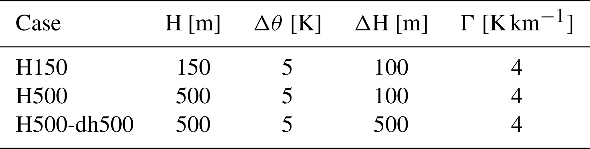
In this section, an overview of the simulation cases and the numerical setup for different solvers is presented. Neutral atmospheric boundary layers (CNBLs) with different BLHs are considered in this study. The boundary layer initialization follows Lanzilao and Meyers (2024), where the initial velocity and potential temperature profiles are generated using the Zilitinkevich (1989) and Rampanelli and Zardi (2004) models, respectively. The geostrophic wind (U_G) is set to 10 m s⁻¹ with a surface roughness (z₀) of $\mathrm{1}\times {\mathrm{10}}^{-\mathrm{4}}$ m. The surface heat flux at the bottom surface is zero according to the CNBL definition.

The BLHs of 150 and 500 m are investigated. These heights are prescribed by the capping inversion height with a strength (Δθ) of 5 K. Moreover, two different capping inversion thickness ΔH values are considered, i.e., 100 and 500 m, for the BLH of 500 m. A free lapse rate (Γ) of 4 K km⁻¹ is applied above the inversion layer. The latitude is set to 55.0°, which represents the latitude of the Doggers Bank offshore wind farm in the North Sea. For reference, the Froude number ($Fr=U_{\mathrm{B}}/\sqrt{g^{\prime }H}$) and the P_N number ($P_{\mathrm{N}}=U_{\mathrm{B}}^{\mathrm{2}}/N{U}_{\mathrm{G}}H$) have been estimated, where U_B is the bulk velocity, calculated from the planar-averaged wind speed in the streamwise direction along the boundary layer height; g^′ is the reduced gravity ($g^{\prime }=g\mathrm{\Delta }\mathit{\theta }/{\mathit{\theta }}_{\mathrm{0}}$); $N=\sqrt{g\mathrm{\Gamma }/{\mathit{\theta }}_{\mathrm{0}}}$ is the Brunt–Väisälä frequency; and H is the boundary layer height (Lanzilao and Meyers, 2024). For the boundary layer height of 150 m, the Fr and P_N numbers are of the order of 1.9 and 5.5, respectively. For a height of 500 m, the values are approximately 1.1 and 1.8, respectively. The parameters for each case are summarized in Table 1.

Table 1 Case definition summary.

The wind farm consists of 100 IEA 15 MW reference turbines (Gaertner et al., 2020) arranged in a 10×10 staggered layout with 5D spacing in both streamwise and spanwise directions, as shown in Fig. 1, resulting in a farm length and width of $L_x^{\mathrm{f}}=\mathrm{10.8}$ and $L_y^{\mathrm{f}}=\mathrm{11.4}$ km, where the x, y, and z axes refer to the streamwise, spanwise, and vertical directions, respectively. The turbine has a rotor diameter (D) of 240 m and a hub height (HH) of 150 m.

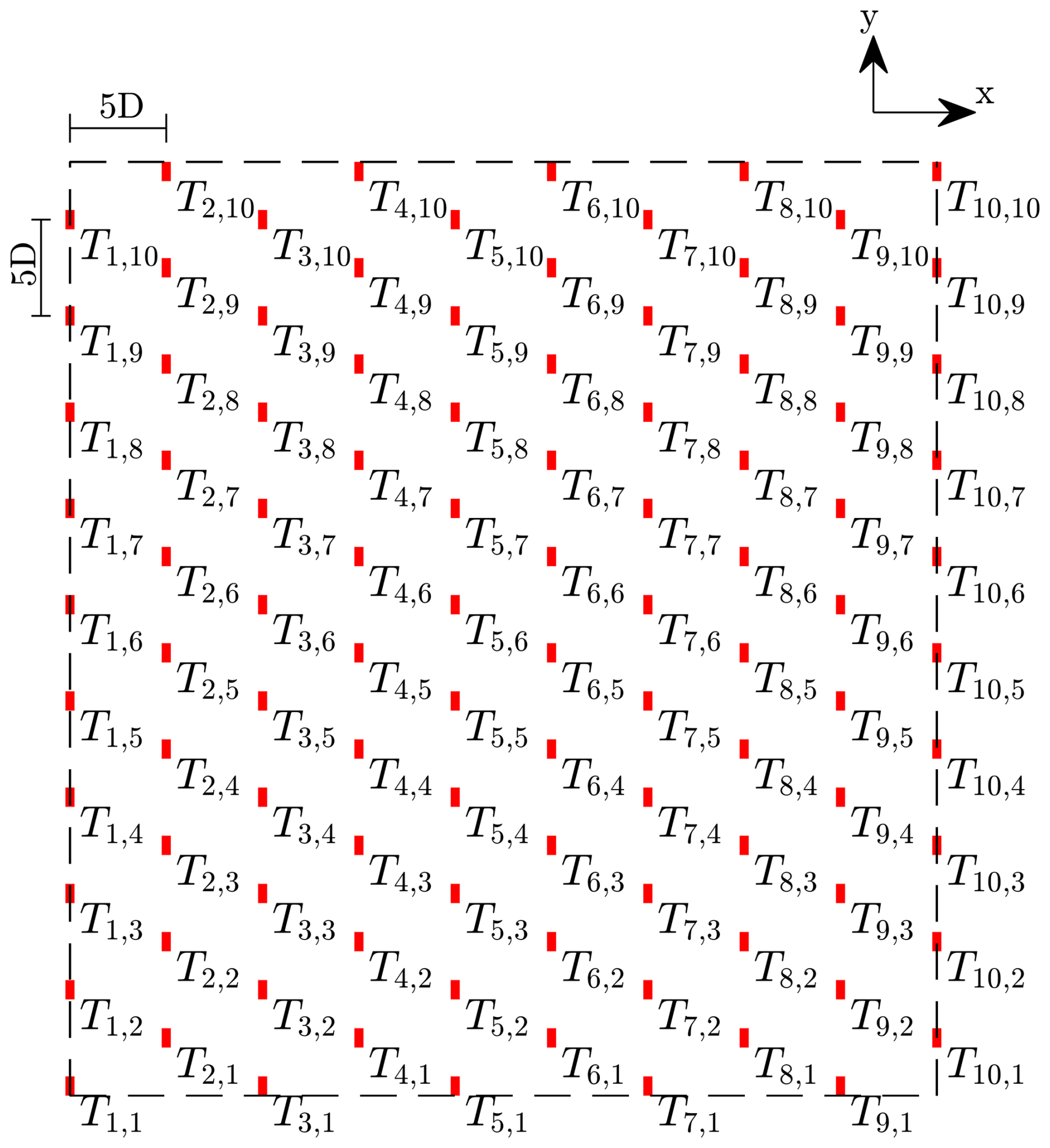
Figure 1 The layout of an idealized wind farm used in this study. Turbines are marked with the letter T, and the subscript numbers indicate the row and column. The x axis refers to the streamwise direction.

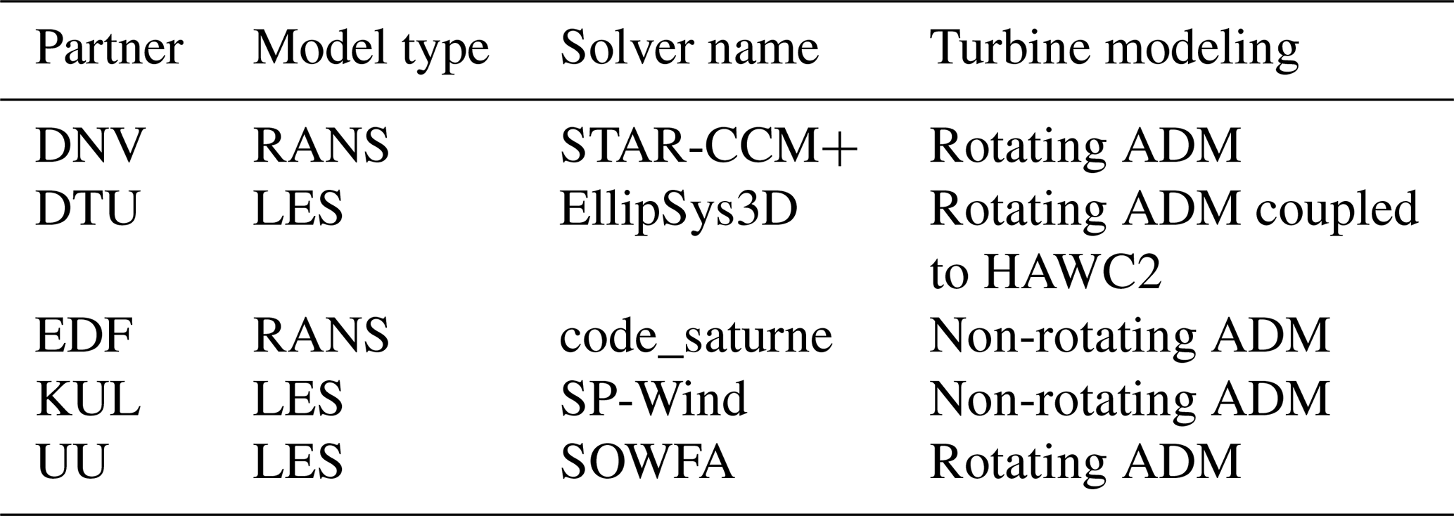
There are five participants from industry and academia, including DNV, Danmarks Tekniske Universitet (DTU), Electricité de France (EDF), Katholieke Universiteit Leuven (KUL), and Uppsala Universitet (UU). The name and type of numerical solvers for each institution, as well as turbine representations, are listed in Table 2.

Table 2 List of participants.

Statistical calculations for the turbulent flow and turbine output of the transient flow solvers are conducted over a physical simulation period of at least 1 h. It should be noted that DTU and UU did not perform the simulation for the H500-dh500 case.

The details of the numerical setup for each solver, such as computational domain, mesh resolutions, boundary conditions, numerical schemes, and turbine modeling, are provided in the following subsections.

2.1 DNV STAR-CCM+ setup

STAR-CCM+ is a general-purpose simulation software package best known for computational fluid dynamics. Within STAR-CCM+, DNV customized a steady-state RANS model for simulation of wind farm flows. The turbulence closure is standard k−ε with modified coefficients. The direct influence of buoyancy on the mean flow is simulated via a shallow Boussinesq formulation; extra terms in the closure equations represent the influence of buoyancy on turbulence. Coriolis terms are in the momentum equation. The turbines are represented with a simple actuator disk model where the body forces are functions of the average axial component of velocity across the disk. These functions are derived from the IEA 15 MW power and thrust curves, defined as functions of hub height freestream wind speed, using the procedure described in Bleeg and Montavon (2022). More information on this flow model can be found in Bleeg et al. (2018).

The simulations in this study were run within a domain of size 66 km × 66 km × 17 km. The wind farm is located 40 km downstream of the inflow boundary. The mesh spacing is 12 m around each actuator disk and 24 m around the wind farm.

Vertical inflow profiles are generated using a steady-state 1D single-column precursor simulation with the input potential temperature profile frozen. After the steady-state simulation converges, the potential temperature is unfrozen, and the 1D solution is marched in time to confirm that the full set of profiles are in quasi-equilibrium.

2.2 DTU EllipSys3D setup

EllipSys3D solves the incompressible Navier–Stokes equations in general curvilinear coordinates using a finite-volume method in a multi-block structure (Michelsen, 1992, 1994; Sørensen, 1995). Rhie–Chow interpolation is applied to prevent pressure decoupling, which is solved using an improved version of the SIMPLEC algorithm (Shen et al., 2003). The convective terms are discretized using a fourth-order central difference scheme, which includes an artificial viscosity term to suppress numerical wiggles (Wit and van Rhee, 2013), and time stepping is performed using a second-order scheme with subiterations. Several RANS and large-eddy simulation (LES) turbulence models are implemented in EllipSys3D, where the anisotropic minimal dissipation (AMD) (Abkar et al., 2016) model has been utilized in the current simulations. Rayleigh damping is applied at high altitudes (> 1000 m).

Initially, a precursor is simulated to spin up the CNBL. The precursor is performed in a domain $L_x\times L_y\times L_z=\mathrm{10}\mathrm{240}$ m ×10 240 m ×3000 m with a total of $N_x\times N_y\times N_z=\mathrm{512}\times \mathrm{512}\times \mathrm{384}\approx \mathrm{100}\times {\mathrm{10}}^{\mathrm{6}}$ cells corresponding to a mesh resolution of $\mathrm{\Delta }x\times \mathrm{\Delta }y\times \mathrm{\Delta }z=\mathrm{20}$ m ×20 m ×5 m in the streamwise, lateral, and vertical directions. The equidistant mesh in the vertical is maintained at an altitude of 1500 m, after which the cells are stretched. Cyclic boundary conditions are imposed in the streamwise and lateral directions, while a wind direction controller is imposed to continuously adjust the wind direction at z=150 m to ensure that the flow direction is aligned with the wind turbines at hub height (Sescu and Meneveau, 2014; Allaerts and Meyers, 2015). The precursor is initially spun up for 20 h, after which cross-stream planes are extracted for a total duration of 2 h.

Subsequently, a mesh is built for the successor, which is $L_x\times L_y\times L_z=\mathrm{30}\mathrm{000}$ m ×30 000 m ×3000 m with a total of $N_x\times N_y\times N_z=\mathrm{512}\times \mathrm{448}\times \mathrm{192}\approx \mathrm{44}\times {\mathrm{10}}^{\mathrm{6}}$ cells. The mesh has a central equidistant region of $L_{x,\mathrm{equi}}\times L_{x,\mathrm{equi}}\times L_{x,\mathrm{equi}}=\mathrm{13}\mathrm{530}$ m ×12 120 m ×1500 with $\mathrm{\Delta }x\times \mathrm{\Delta }y\times \mathrm{\Delta }z=\mathrm{30}$ m ×30 m ×10 m in the streamwise, lateral, and vertical directions with cells stretched to the boundaries. The precursor planes have been repeated to cover the extended domain of the successor simulations. The wind turbines are modeled by applying body forces in EllipSys3D, which is fully coupled to the aero-elastic tool HAWC2 (Larsen and Hansen, 2007) through the Dynamiks interface (https://dynamiks.pages.windenergy.dtu.dk/dynamiks/index.html, last access: 10 February 2026). Velocities are transferred from EllipSys3D to HAWC2, which calculates aerodynamic forces and deflections, which are transferred back to EllipSys3D (Sørensen et al., 2015; Hodgson et al., 2022, 2023). HAWC2 also contains a dynamic torque controller, which enables the turbines to respond to the dynamically changing inflow by dynamically updating pitch and rotational speed, but it does not yaw the turbines. The impact of realistic and dynamic wind turbine controllers has been shown to have a significant influence on power production for wind farms (Troldborg and Andersen, 2023). Turbines can be modeled as actuator lines (Sørensen and Shen, 2002) or as actuator disks (Mikkelsen, 2004), which is used in this study. The simulations are run for 2 h, where the initial 1 h transient is discarded as the flow is still developing.

2.3 EDF code_saturne setup

The CFD code code_saturne, primarily developed by EDF, is an open-source, free-to-use finite-volume CFD solver for the Navier–Stokes equations. It can manage scalar transport for various types of flows – 2D, 2D axisymmetric, 3D, steady, unsteady, laminar, turbulent, incompressible, dilatable, weakly compressible, or isothermal. Code_saturne comes with modules specifically designed for certain physics, such as atmospheric flows. An extensive explanation of its modeling capabilities, including the atmospheric module, can be found in code_saturne’s v8.0 online theory guide (https://www.code-saturne.org/documentation/8.0/theory.pdf, last access: 10 February 2026).

Reynolds-averaged Navier–Stokes (RANS) with linear production k−ε closure (Guimet and Laurence, 2002) is used to model turbulence. The presence of wind turbines is accounted for using a non-rotating ADM with a constant body force function of the disk-averaged velocity and yaw control.

Wind farm simulations with code_saturne are performed in two steps. The first step consists of a 1D bi-periodic single-column precursor simulation to generate quasi-steady inflow profiles for the velocity, temperature, and turbulent quantities. The second step consists of the full 3D farm simulation in a circular domain with a refined grid in the farm and around turbines. The numerical domain is 25 km high, and a diameter as large as 4.7 times the length of the longest diagonal of the farm was shown to be sufficient to avoid confinement effects. Damping layers at the top and at lateral boundaries are implemented to prevent the reflection of gravity waves.

2.4 KUL SP-Wind setup

The SP-Wind flow solver is in-house software developed over the past 15 years at KU Leuven (Meyers and Sagaut, 2007; Calaf et al., 2010). In the current study, we use this software to solve the filtered Navier–Stokes equations with a Boussinesq approximation coupled with a transport equation for the potential temperature to investigate the flow in and around a large-scale wind farm (Allaerts and Meyers, 2017; Lanzilao and Meyers, 2022, 2023). Here, we adopt the same solver version used by Lanzilao and Meyers (2024), which is described below.

The governing equations are integrated in time using a classic fourth-order Runge–Kutta scheme, with the time step determined by a Courant–Friedrichs–Lewy (CFL) number of 0.4. The streamwise (x) and spanwise (y) directions are discretized using a Fourier pseudo-spectral method. This approach involves discretizing all linear terms in the spectral domain while performing non-linear operations in the physical domain, which reduces the computational cost of convolutions from quadratic to log-linear (Fornberg, 1996). Additionally, the $\mathrm{3}/\mathrm{2}$ dealiasing technique from Canuto et al. (1988) is employed to prevent aliasing errors. For the vertical dimension (z), an energy-preserving fourth-order finite-difference scheme is utilized (Verstappen and Veldman, 2003). The impact of subgrid-scale motions on the resolved flow is modeled using the stability-dependent Smagorinsky model (Stevens et al., 2000), with the Smagorinsky coefficient C_s set to 0.14. Near the wall, this coefficient is damped using the function proposed by Mason and Thomson (1992). Continuity is maintained by solving the Poisson equation at each stage of the Runge–Kutta scheme. We refer to Delport (2010) for more details on the discretization of the continuity and momentum equations, while the implementation of the thermodynamic equation and subgrid-scale model are explained in detail in Allaerts (2016).

The flow solver adopts two numerical domains simultaneously marched in time: the precursor and main domains. The precursor domain, which does not contain turbines, has the function of generating a fully developed, statistically steady turbulent flow. This flow is then used to drive the simulation in the main domain. Following the approach in Allaerts and Meyers (2017, 2018a) and Lanzilao and Meyers (2024), the precursor domain dimensions are set to $L_x^{\mathrm{p}}=L_y^{\mathrm{p}}=\mathrm{10}$ km and $L_z^{\mathrm{p}}=\mathrm{3}$ km. The wind farm is situated in the main domain, which must be sufficiently large to avoid artificial effects from domain boundaries. Lanzilao and Meyers (2024) have shown that the width of the numerical domain can significantly alter the numerical results. To this end, we fix the main domain size to $L_x\times L_y=\mathrm{50}\times \mathrm{40}$ km², which leads to a domain-to-farm width ratio of 3.51. Consistent with previous studies, the main domain height is set to L_z=25 km (Allaerts and Meyers, 2017, 2018a; Lanzilao and Meyers, 2022, 2023, 2024). This vertical extent allows gravity waves to dissipate and radiate energy outward, minimizing reflectivity. After completing the precursor spin-up phase, the precursor domain width and height are extended to match the main domain dimensions, using the method described in Sanchez Gomez et al. (2023) and Lanzilao and Meyers (2024). To reach a statistically steady state, the flow fields in the precursor simulation are marched in time for 20 h. These flow fields are used to drive the main domain, where a second spin-up phase of 1 h takes place so that the flow adjusts to the presence of the turbines. Next, the wind-angle controller, which keeps the flow aligned with the streamwise direction at hub height, is switched off, and statistics are collected over a time window of 2 h.

In regard to the grid resolution, we fix Δx=31.25 m and Δy=21.74 m in the streamwise and spanwise directions, respectively. This leads to N_x=1600 and N_y=1840 grid points for the main domain and $N_x^{\mathrm{p}}=\mathrm{160}$ and $N_y^{\mathrm{p}}=\mathrm{230}$ points for the precursor domain. In the vertical direction, we adopt a stretched grid, which corresponds to the one used in Lanzilao and Meyers (2022, 2023, 2024), i.e., with a resolution of 5 m within the first 1.5 km and stretched above, for a total of 490 grid points. The combination of precursor and main domains leads to a total of roughly 6.92×10⁹ degrees of freedom (DOFs).

At the top of the domain, we use the Rayleigh damping layer (RDL) to minimize gravity-wave reflection (Klemp and Lilly, 1977). To avoid periodicity in the streamwise direction, we adopt the wave-free fringe-region technique developed by Lanzilao and Meyers (2023). The buffer layer setup corresponds to the one previously used by Lanzilao and Meyers (2024). Hence, the RDL is 10 km thick and is located between z=15 and z=25 km. Moreover, ν^ra=5.15 and s^ra=3 are parameters used in the RDL. The fringe region is 5.5 km long and is located at the end of the main domain. Further, we set $x_s^h=L_x-L_x^{\mathrm{fr}}$, $x_e^h=L_x-\mathrm{2.8}$ km, and ${\mathit{\delta }}_s^h={\mathit{\delta }}_e^h=\mathrm{0.4}$ km, while $x_s^d=x_s^h$, $x_e^d=L_x$, ${\mathit{\delta }}_s^d=\mathrm{2.5}$ km, and ${\mathit{\delta }}_e^d=\mathrm{3}$ km. Finally, we fix the strength of the forcing to h_max=0.3 s⁻¹.

The turbine drag force is represented with the non-rotating actuator disk model (Calaf et al., 2010), where the power is computed as the product between the thrust force and the turbine disk velocity. We use a constant thrust coefficient value of 0.778, which corresponds to a $C_{\mathrm{T}}^{\prime }$ of 1.44. A simple yaw controller is implemented to keep the turbine rotor disks perpendicular to the incident wind flow measured 1 rotor diameter upstream.

2.5 UU SOWFA setup

The Simulator fOr Wind Farm Applications (SOWFA) was developed by NREL (Churchfield et al., 2012). It is built on the OpenFOAM software, an open-source finite-volume solver that can be coupled to an aeroelastic code for turbine load and control study. Turbulent winds and wakes are modeled using LES with the one-equation eddy viscosity subgrid-scale model (Deardorff, 1980).

The domain extent is set to $L_x\times L_y\times L_z=\mathrm{26}\mathrm{400}$ m ×32 000 m ×6000 m with a mesh resolution of $\mathrm{\Delta }x\times \mathrm{\Delta }y\times \mathrm{\Delta }z=\mathrm{20}$ m ×20 m ×8 m up to a height of 720 m. The mesh generation was carried out by dividing the domain into four horizontal layers, with the mesh vertically stretched and a larger expansion ratio applied to the upper layers to reduce computational cost. This results in approximately 235 million cells in the domain.

There are two steps in the simulations. The first step is the precursor simulation, in which the turbulent ABLs are generated. A periodic boundary condition is applied to all lateral boundaries for an empty flow domain, where the horizontal driving pressure gradient is adjusted at every time step to control the mean wind speed and direction at the hub height (Churchfield et al., 2012). This is done by determining the source term from the error between the actual planar-averaged velocity at the specified height and the desired velocity. This approach is suitable for turbine engineering analyses in which the hub height wind speed can be prescribed. However, it is acknowledged that this method cannot simultaneously achieve both the desired geostrophic wind vector and the hub height wind direction. The Schumann wall shear stress model is used for wall modeling at the bottom surface, while the top boundary is a free-slip wall. The precursor simulation is performed until the turbulent flow reaches a quasi-steady state before the flow data on a cross-flow plane are recorded to be used as the inflow for the wind farm simulations.

The second step is the wind farm simulation, in which the streamwise boundaries are changed to inlet and outlet boundary conditions. The bottom and top boundaries are identical to those of the precursor simulation. The turbines are modeled using an actuator disk method with a simple controller in which the rotor speed and pitch angle are functions of the average axial velocity across the rotor (Troldborg and Andersen, 2023). The aerodynamic forces and power of the rotors are calculated using the blade element method. A simple yaw controller is implemented to keep the rotor facing local wind directions. The statistical calculations for the turbulent flow and turbine output are performed over the last hour of the simulation time after the initial pass.

3 Results

The numerical results from different numerical solvers are compared in the following subsections. The results include inflow conditions, wind farm flows, wind farm performance, and wind farm efficiency.

3.1 Inflow profiles

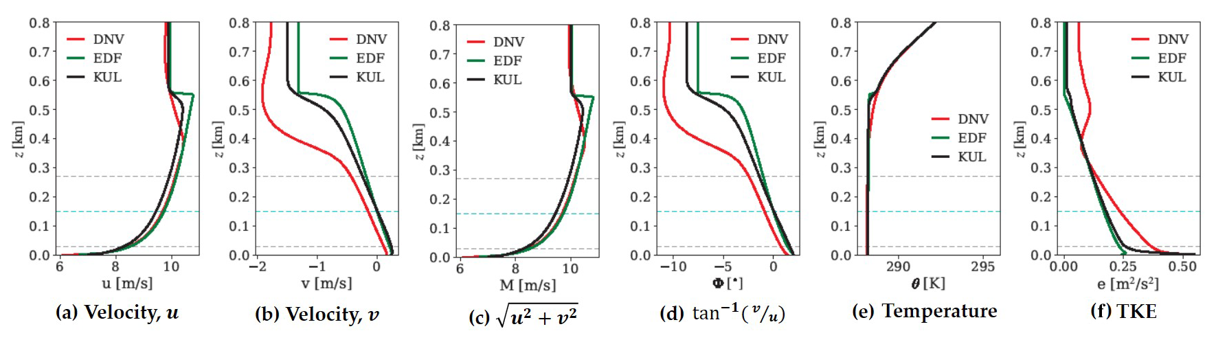
As mentioned in Sect. 2, each participant uses different approaches to obtain atmospheric flows. Figures 2–3 illustrate the vertical inflow profiles generated by the different solvers, where u and v are velocity components in the streamwise and spanwise directions, respectively; M corresponds to the magnitude of horizontal wind velocity vectors; Φ denotes the wind angle between the wind vector and the x axis; Θ is potential temperature; and e corresponds to the turbulent kinetic energy (TKE).

Figure 2 Inflow profiles of the H150 case.

Figure 3 Inflow profiles of the H500 case.

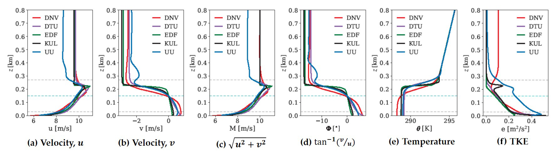
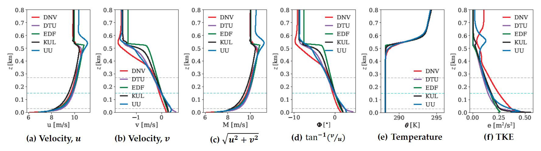
In general, all solvers produce similar inflow profiles near the rotor height. The velocity profile of the H150 case exhibits a low-level jet-like shape where the peak of supergeostrophic wind speeds is observed close to 200 m height. Wind veering is also significant in the H150 case, where the wind direction difference between the top and bottom of the rotor is almost 15°, while it is less than 5° in the H500 and H500-dh500 cases.

It should be noted that UU may not achieve the geostrophic wind speed of 10 m s⁻¹ because the mean wind speed and direction are controlled at the hub height, as presented in Sect. 2.5. Furthermore, it was challenging to achieve quasi-steady state for UU due to the initial oscillation of the wind speeds above the capping inversion. The main deviations considering veer, potential temperature, and turbulence kinetic energy are in Fig. 2f, where the SOWFA setup differs due to its inability to resolve the smallest scales because of the required numerical cost. However, this problem does not affect the results in Fig. 4f, where the deeper boundary layer has less wind shear. There are no significant differences for the velocities and TKE profiles between the H500 and H500-dh500 cases; only the potential temperature profile differs due to the initial capping inversion thickness (Figs. 4 and 3).

Figure 4 Inflow profiles of the H500-dh500 case.

Another notable outlier is the DNV potential temperature profile for the H150 case. As can be seen in Fig. 2e, the inversion in the DNV profile is thicker and starts at a lower height compared with the other simulations. The precursor simulations for all the models started from the same potential temperature profile, with the inversion starting at 150 m and a ground potential temperature of 288.15 K, but the DNV precursor approach preserves the initial potential temperature profile to a greater degree than the other approaches, resulting in material differences in the conditions at the simulated wind farms. The DNV created a second set of inflow profiles from a precursor simulation using a potential temperature profile that is more consistent with the inflow profiles from the other four contributors; this second set of H150 profiles (not shown) is much more similar to the other profiles, particularly the wind speed and wind direction profiles.

3.2 Wind farm flows

The mean streamwise velocity, averaged across the wind farm width at hub height, is presented in Fig. 5 from 25D upstream to 65D downstream of the first row of turbines. Overall, all solvers indicate a more significant decrease in the wind speed in the H150 case compared to the H500 and H500-dh500 cases. To quantify and compare wake recovery, mean wind speeds are normalized by the wind speed 25D upstream of the wind farm, as shown in Fig. 6. For the H150 case, EDF, KUL, DTU, and UU predict a similar wake recovery rate, with velocity reductions of approximately 30 %–40 % relative to the freestream winds, while DNV estimates a reduction over 40 %. For the H500 case, UU overpredicts wake recovery compared to EDF, KUL, and DNV, while DTU switches between following the trend of UU and that of the other models. The H500-dh500 case shows similar trends to the H500 case, which thus suggests that the capping inversion thickness does not significantly affect the wind farm wake flows.

Figure 5 Mean streamwise velocity averaged over the wind farm width at hub height.

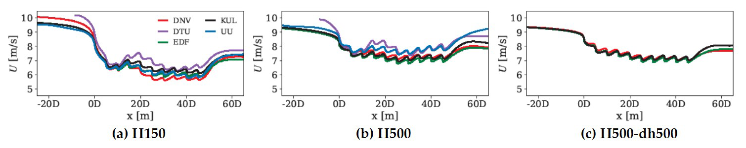
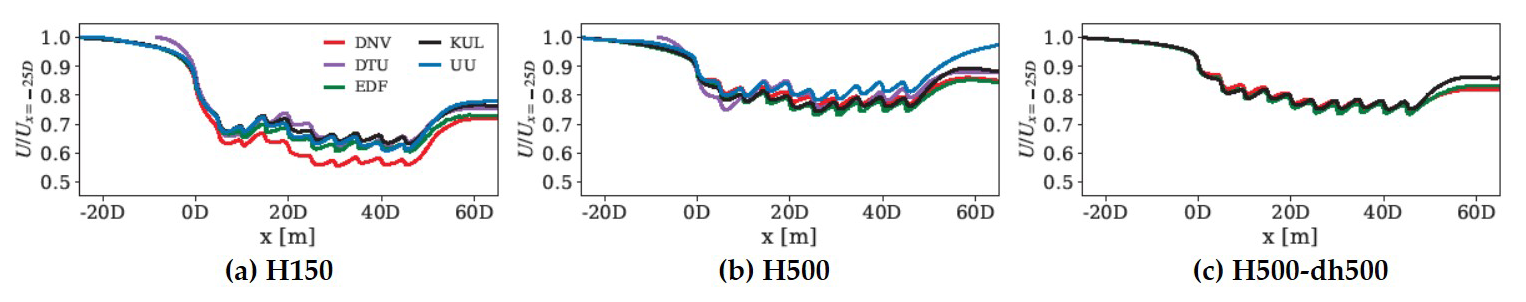
Figure 6 Normalized mean streamwise velocity averaged over the wind farm width at hub height.

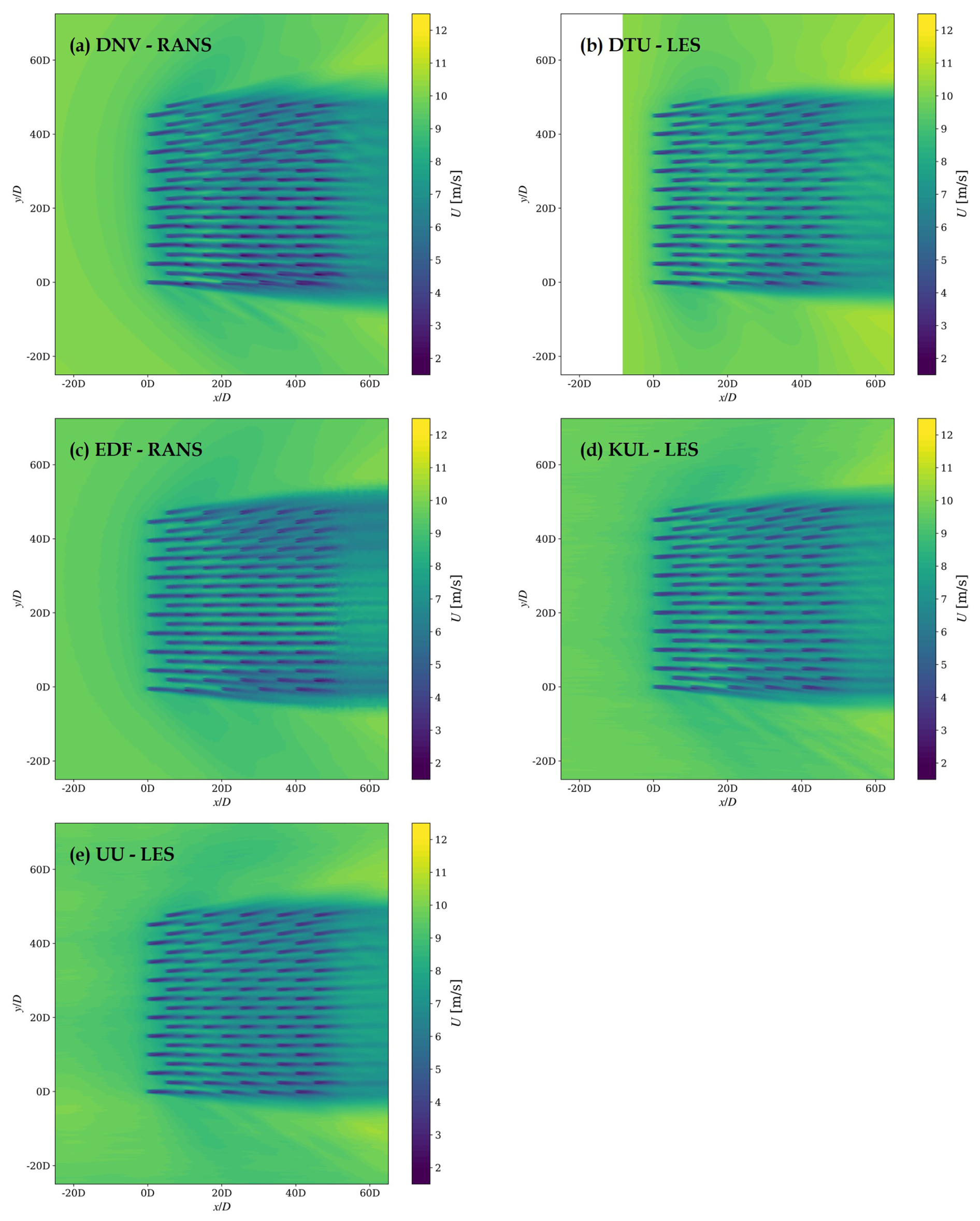
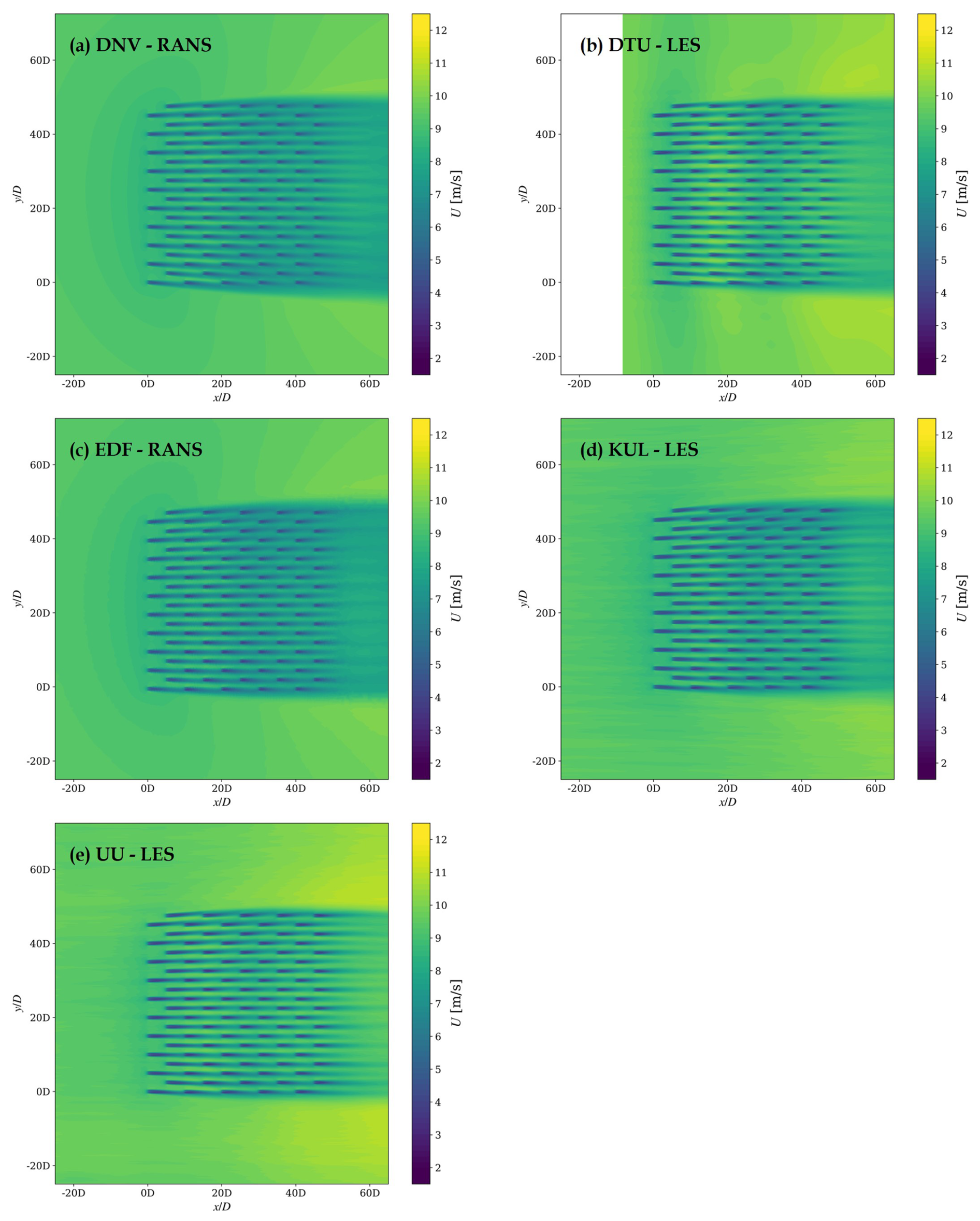
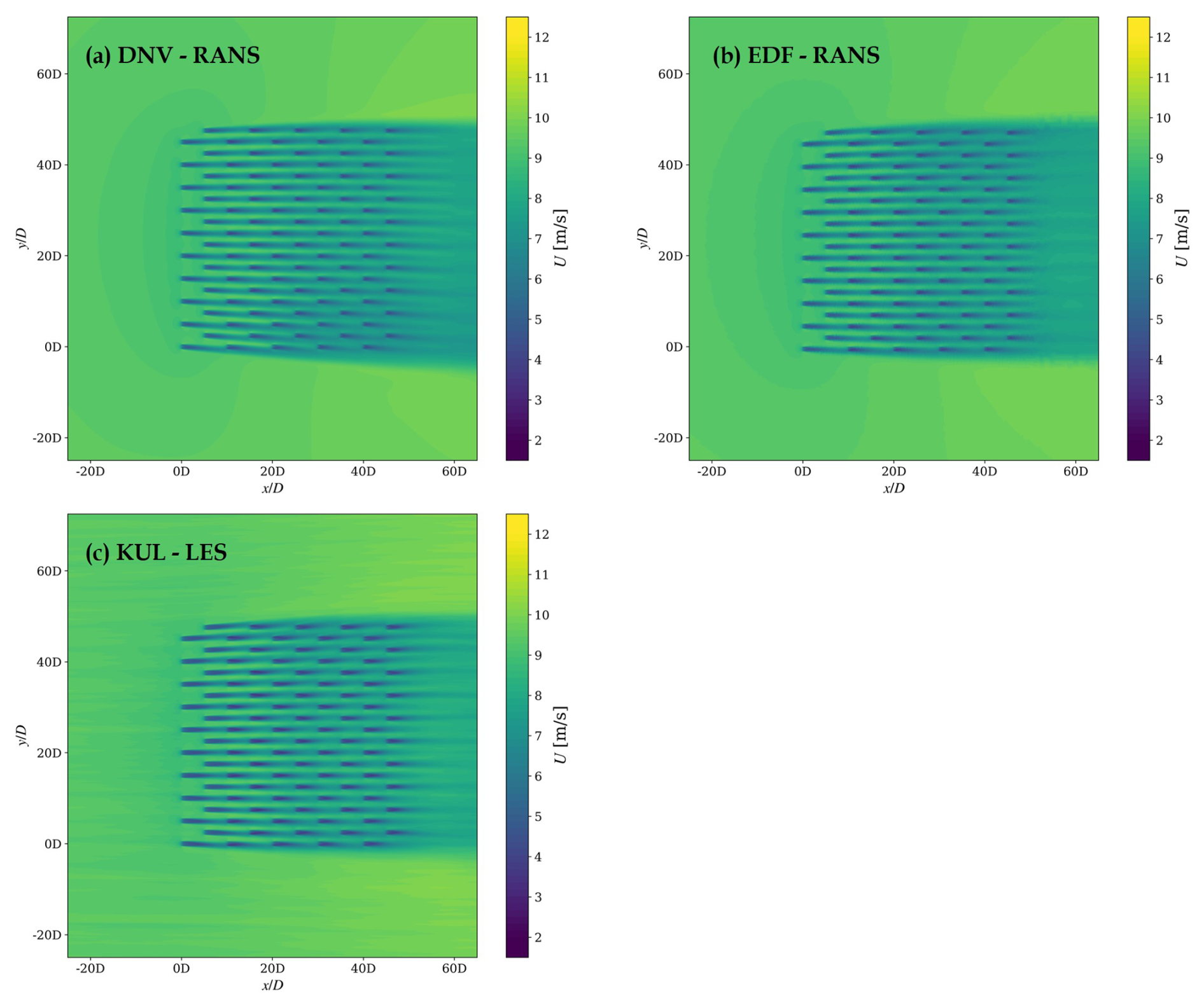
Figures 7–9 show the streamwise velocity contours for the H150, H500, and H500-dh500 cases, respectively, in an x–y plane at hub height. In the H150 case (Fig. 7), the shallow boundary layer restricts the flow above the wind farm, and this leads to a stronger deflection of the wakes at the edges of the farm compared to the 500 m BLH cases shown in Figs. 8 and 9.

Figure 7 Mean streamwise velocity on the X–Y plane at hub height for the H150 case.

Figure 8 Mean streamwise velocity on the X–Y plane at hub height for the H500 case.

Figure 9 Mean streamwise velocity on the X–Y plane at hub height for the H500-dh500 case.

The stronger wind veering in the shallow boundary layer results in more pronounced skewed wakes, as illustrated in a cross-flow (y–z) plane 10D downstream of the last row of turbines (Figs. 10, 11, and 12).

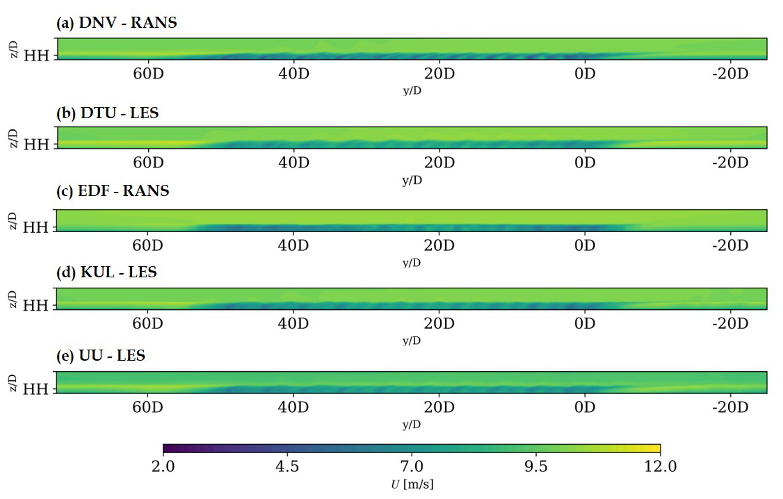
Figure 10 Mean streamwise velocity on the X–Z plane 10D downstream of the last row for the H150 case, viewed from downstream.

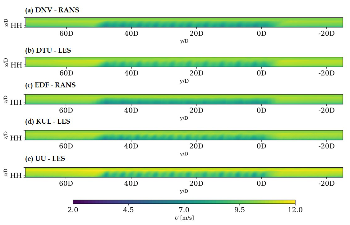
Figure 11 Mean streamwise velocity on the Y–Z plane 10D downstream of the last row for the H500 case, viewed from downstream.

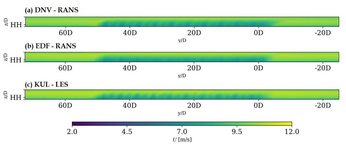
Figure 12 Mean streamwise velocity on the Y–Z plane 10D downstream of the last row for the H500-dh500 case, viewed from downstream.

Further wind speed comparisons on the x–z and y–z planes can be found in Appendix B.

3.3 Wind farm performance

The performance of the wind farm is quantified and compared using power output and turbine yaw angle. Figures 13–15 illustrate the row-averaged power output for each case, including absolute power output, power normalized by the first row ($P/P_{\mathrm{1}}$), and power normalized by an isolated turbine output ($P/P_{\mathrm{\infty }}$). It is noted that the isolated turbine output data for all solvers can be found in Appendix A. For the H150 case, all solvers give a similar row-averaged power output trend where the power reduces by approximately almost 20 % in the second row. For instance, the $P/P_{\mathrm{\infty }}$ of the second rows (Figs. 13c, 14c, and 15c) are approximately 60 % for the H150 case and more than 70 % for the H500 and H500-dh500 cases. Even though this is a staggered-layout wind farm where the second row is not directly in the wake of the first row, this significant power reduction in the second row indicates a strong blockage effect in the H150 case compared to the other cases. The power drops further in the third row before it recovers in the fourth and fifth rows. Since DTU and UU did not simulate the H500-dh500 case, fewer results are available for comparison, which makes the results in Fig. 15 appear less distinct than those in Figs. 13 and 14.

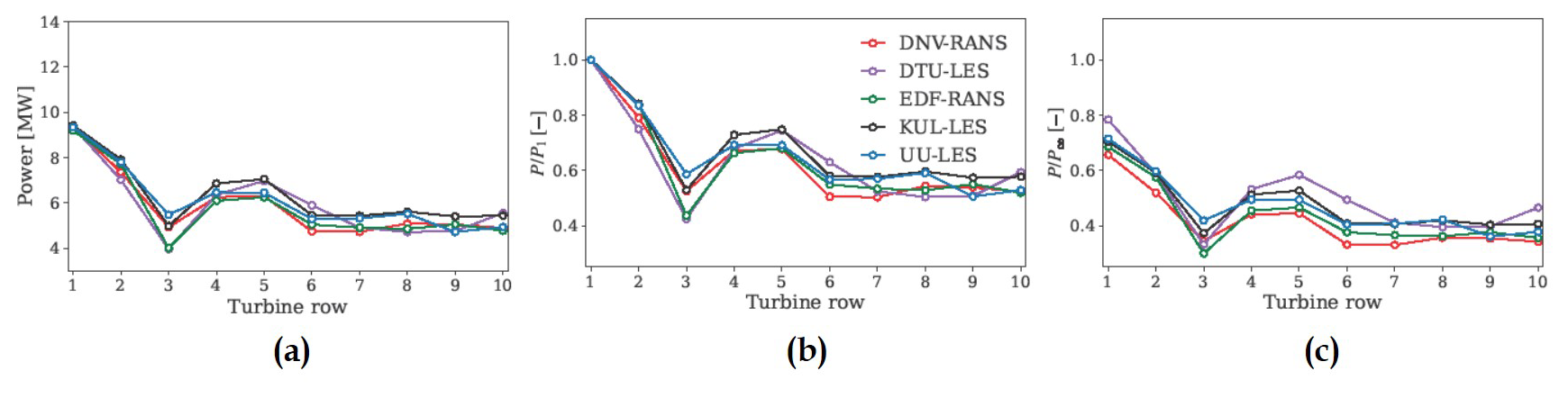
Figure 13 Row-averaged power output for the H150 case: (a) absolute power output, (b) power output normalized by the first row, and (c) power output normalized by an isolated turbine power.

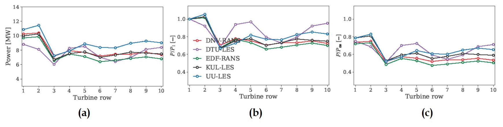
Figure 14 Row-averaged power output for the H500 case: (a) absolute power output, (b) power output normalized by the first row, and (c) power output normalized by an isolated turbine power.

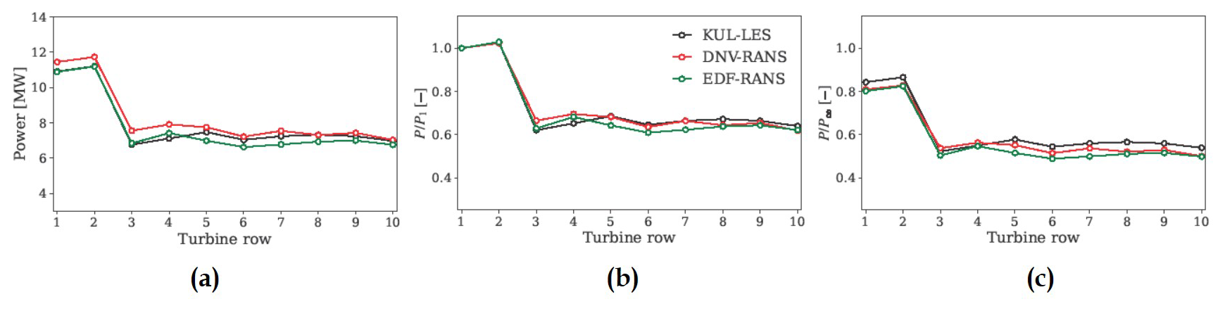
Figure 15 Row-averaged power output for the H500-dh500 case: (a) absolute power output, (b) power output normalized by the first row, and (c) power output normalized by an isolated turbine power.

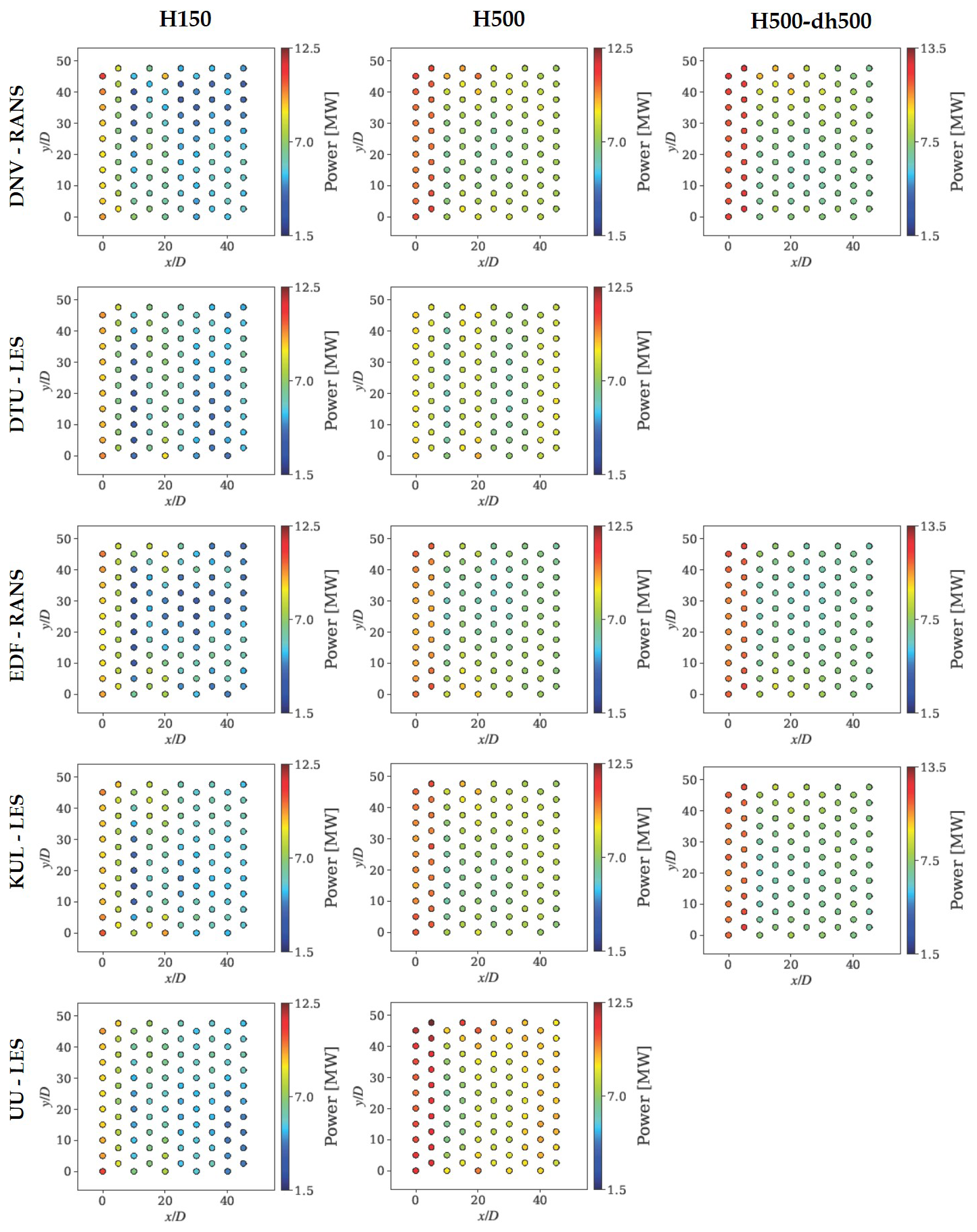
The power distribution in the farm is depicted in Fig. 16. The left, middle, and right columns represent the H150, H500, and H500-dh-500 cases, respectively. In all cases, the turbines near the edges of the front rows generate more power than the turbines in the middle.

Figure 16 The power distribution in the farm is depicted.

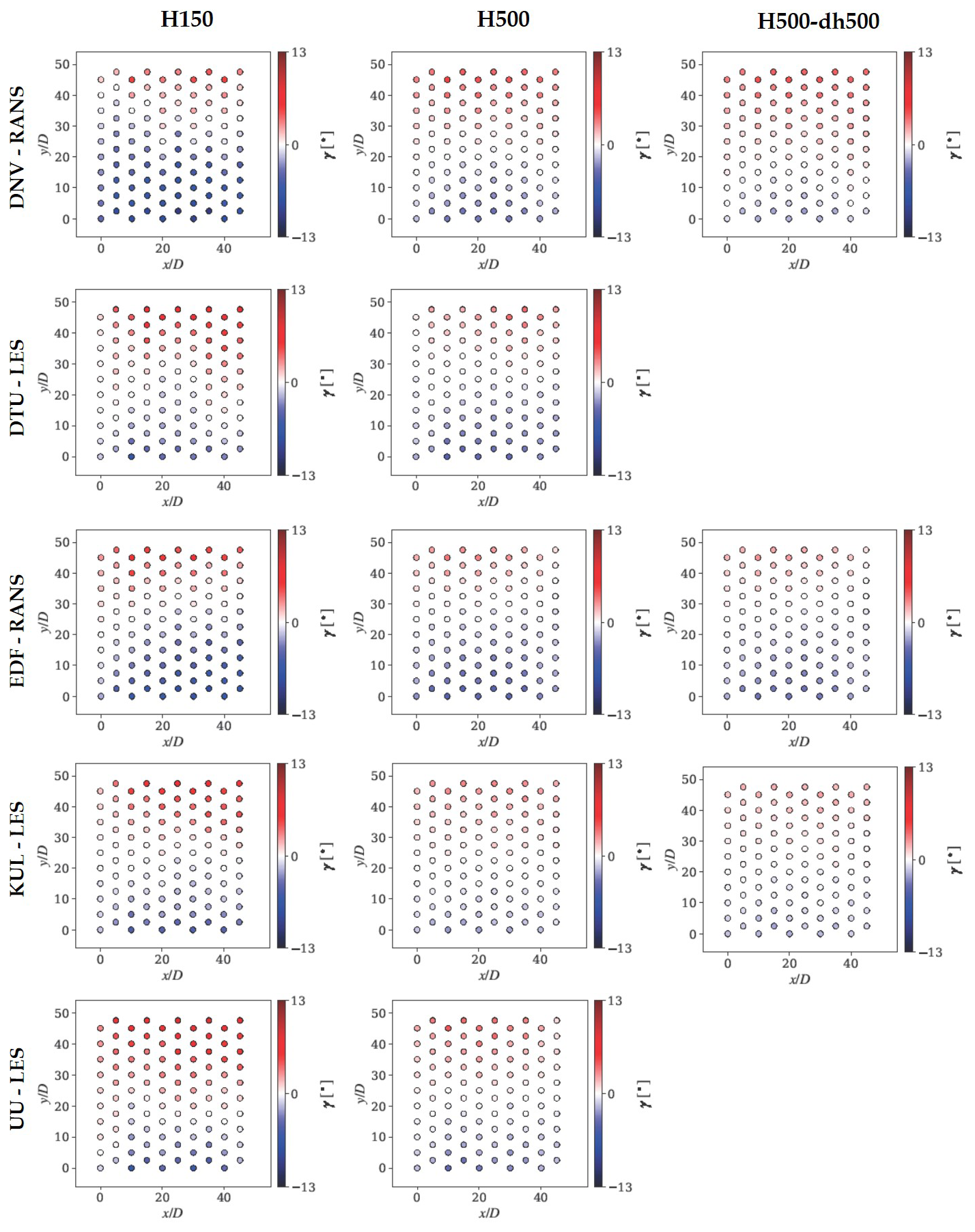
The averaged turbine yaw angles are presented in Fig. 17. Each turbine in the farm responds to the local wind direction by yawing the rotor to maximize the power output. For the H150 case, the more pronounced spanwise flows cause the turbines close to the sides of the farm to yaw more significantly where the averaged yaw angles are more than 10°.

Figure 17 Local wind direction.

3.4 Wind farm efficiencies

Wind farm power production losses due to blockage and wake interactions are quantified by the following definitions as introduced by Allaerts and Meyers (2018b). Losses due to wake interactions or wake efficiency (η_w) can be expressed as

$$\begin{array}{}\text{(1)}& {\mathit{\eta }}_{\mathrm{w}}={\displaystyle \frac{P_{\text{tot}}}{N{P}_{\mathrm{1}}}},\end{array}$$

where P_tot describes the total wind farm power output, N is the number of turbines in a farm, and P₁ is the power of front-row turbines. The losses due to non-local effects, i.e., the blockage effect, can be expressed as

$$\begin{array}{}\text{(2)}& {\mathit{\eta }}_{\mathrm{nl}}={\displaystyle \frac{P_{\mathrm{1}}}{P_{\mathrm{\infty }}}},\end{array}$$

where P_∞ is obtained from single-turbine simulations. The total wind farm efficiency (η_farm) is then the product of losses introduced by non-local and wake effects:

$$\begin{array}{}\text{(3)}& {\mathit{\eta }}_{\text{farm}}={\mathit{\eta }}_{\mathrm{w}}{\mathit{\eta }}_{\mathrm{nl}}.\end{array}$$

The efficiencies calculated from Eqs. (1), (2), and (3) are summarized in Tables 3, 4, and 5. The results indicate that wind farm efficiency is highly dependent on the depth of the boundary layer. In the H150 case, losses from wake interaction can reach nearly 40 %, while in the H500 case, they are around 20 %. Furthermore, due to the blockage effect, the front-row turbines can generate approximately 70 % and 80 % of the output of an isolated turbine in shallow and deeper boundary layers, respectively.

Table 3 Wind farm efficiencies for the H150 case.

Table 4 Wind farm efficiencies for the H500 case.

Table 5 Wind farm efficiencies for the H500-dh500 case.

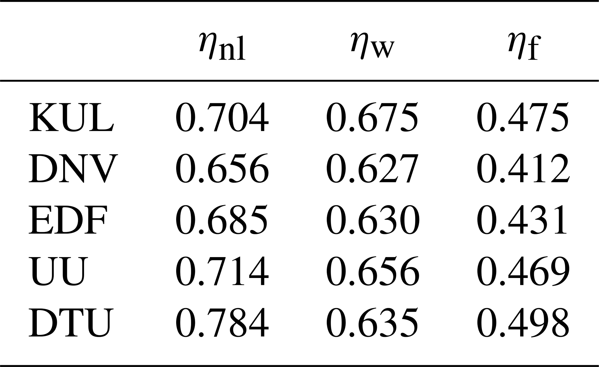
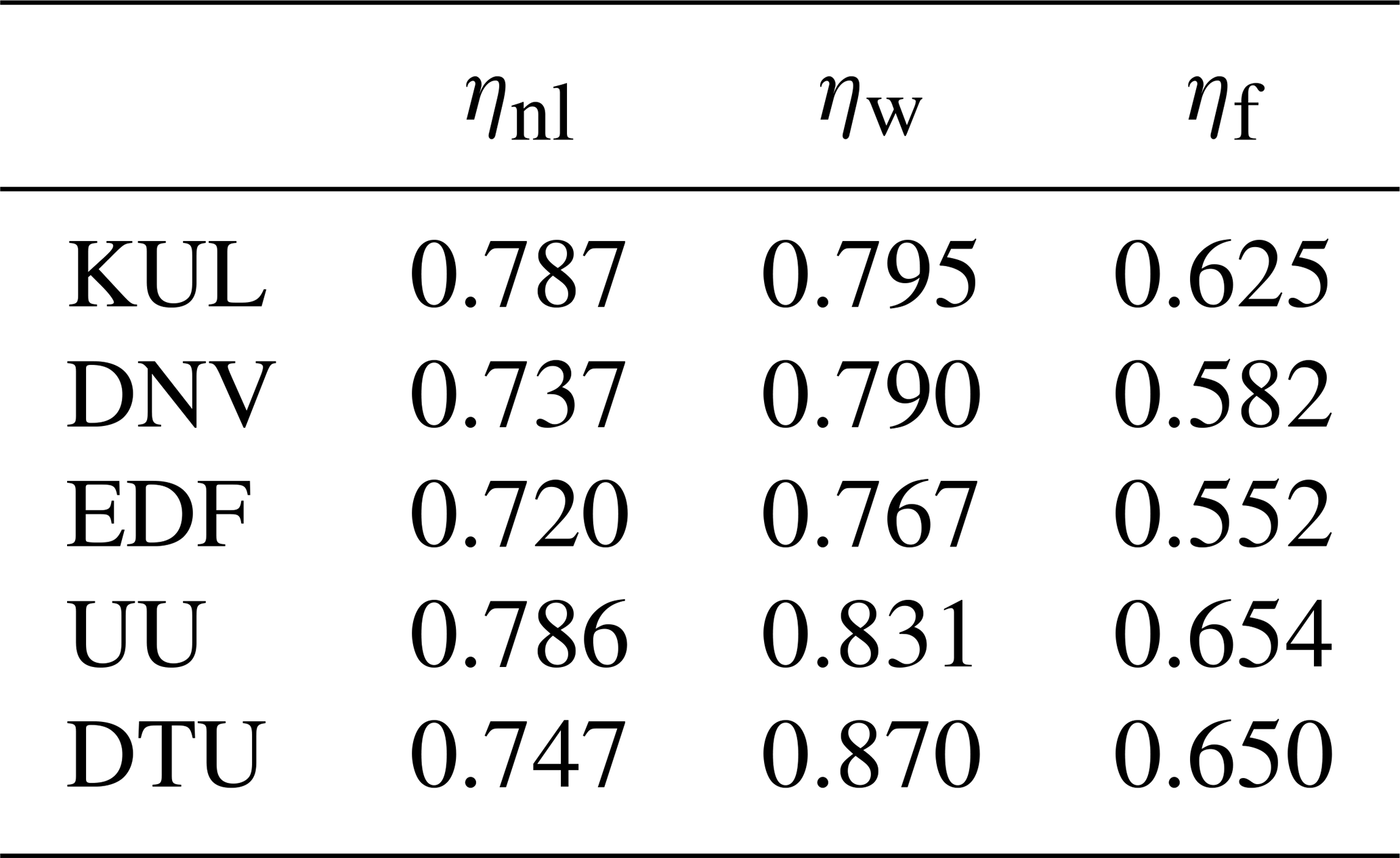
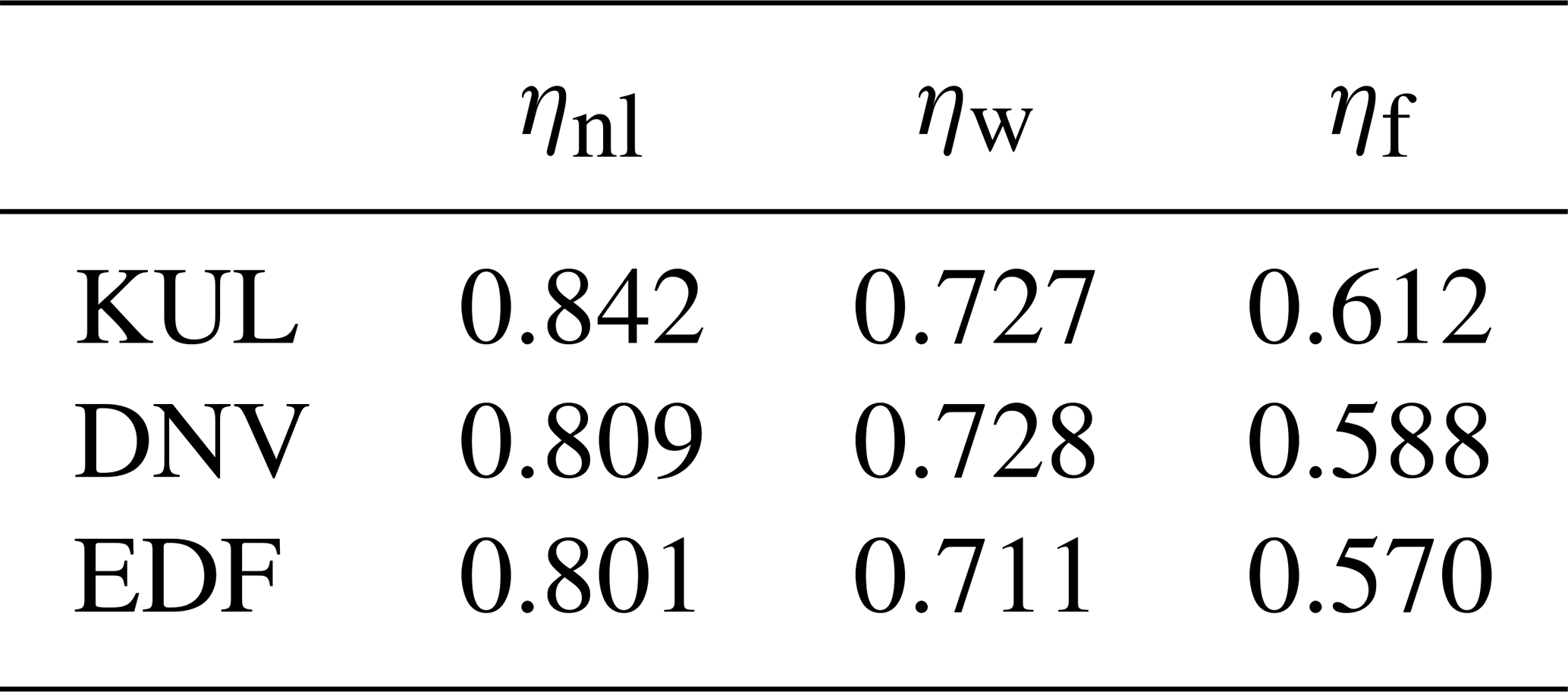
The efficiencies also reveal the influence of capping inversion thickness on wind farm performance. Results from DNV, EDF, and KUL show that the case with a thicker capping inversion leads to a reduced blockage effect but slightly larger wake losses compared to the thinner capping inversion.

The DNV H150 results are an outlier relative to the other models, with lower relative wind speeds throughout the wind farm (Fig. 6a) and lower wind farm efficiency (Table 3). The gap between the DNV wind farm calculation and the other calculations for this case is simply a consequence of simulating a different potential temperature profile, which corresponds to a thinner boundary layer. When the DNV H150 case is rerun with inflow profiles that are more consistent with those of the other contributors, the wind speeds throughout the farm (not shown) and the calculated efficiencies (η_nl=0.695, η_w=0.620, and η_farm=0.431) are more like the results from the others. The level of agreement is similar to how the DNV results compare with other results for the H500 and H500-dh500 cases. Thus, the outlier wind farm predictions from DNV presented for the H150 case have more to do with inflow conditions than differences between the models.

We here would like to highlight that the level of non-local blockage depends on the simulated conditions and selected dense wind farm layout. In this case, the power density is approximately 12 MW km⁻². This is in the range of the Belgium offshore economic zone and the German Bight but is denser compared to Danish and UK offshore cases.

In addition, the calculated efficiencies are a lot lower than would be calculated in an energy yield analysis, which would involve simulations over a much broader range of conditions, including wind directions and wind speeds where the efficiencies are at or very close to 1.0. However, our focus is not on the overall AEP calculations but rather on the quality and comparison of codes to represent wind farm flows under strong-blockage conditions.

4 Discussion

Based on the results presented in Sect. 3, there are a few issues that need to be discussed further. Firstly, there are discrepancies in the inflow profiles generated by the different numerical approaches because the simulations were set up according to the best practice of each solver to match the specified atmospheric conditions. The geostrophic winds generated by UU do not match those of other solvers at 10 m s⁻¹ due to the wind speed and direction control approach. UU also overestimated the TKE for the H150 case due to the relatively coarse mesh resolution in the LES precursor. However, key features, including wind shear, wind veer, and potential temperature, are comparable. It should be noted that the aim of this study was not to provide a code-to-code comparison to verify flow solvers. In order to conduct a proper code comparison, reference inflow conditions, i.e., met mast or lidar data, should be available for validation (Doubrawa et al., 2020; Asmuth et al., 2022). Instead, the purpose of this study is to illustrate the impact of the BLH and capping inversion thickness on a large-wind-farm operation using various numerical approaches. The results of different fidelity models, stretching from RANS to LES, show convincing trends in wind farm performance and highlight the importance of the BLH.

Another source of difference between the simulation tools is the turbine representation, as described in Sect. 2. The turbine-induced aerodynamic forces differ, as KUL and EDF used a non-rotating disk model, while DNV, DTU, and UU used a rotating disk model. It is difficult to isolate the impact of this discrepancy in the current set of simulations, as other factors, such as differences in inflow conditions and mesh resolutions, are also involved. Some previous studies have demonstrated that the choice between non-rotating and rotating disk methods may only affect the near-wake profile, while both models yield good agreement in the far wake (Meyers and Meneveau, 2010; Wu and Porté-Agel, 2011; van der Laan et al., 2015). However, the impact of turbine-induced force distribution on wind farm efficiency, particularly a dense wind farm, has yet to be verified. Furthermore, the turbine controllers also differ among the tools: EDF and KUL used a constant thrust coefficient, DNV and UU used an averaged disk velocity to reference tabulated data, and DTU simulated a full controller within an aeroelastic code. These differences cause the turbines to respond differently to the incoming flows. For instance, DTU's full controller is capable of simulating a more realistic turbine response under varying wind shear and wind veer in the H150 and H500 cases, as the variable speed and pitch are controlled using the instantaneous torque on the disks as the input signal. However, the simpler controllers used by DNV and UU may underestimate the impact of varying velocity shear and directional veer on the turbine power output due to the averaging of rotor disk velocity. This issue is particularly significant for the large rotor size of the 15 MW turbine, as it can cause the turbines to respond differently to the incoming flows, and using a static or dynamic controller can significantly impact the estimated power production (Troldborg and Andersen, 2023). Nevertheless, although it is important to acknowledge these differences in turbine models, we would like to emphasize that the single-turbine simulations that were used to normalize results (e.g., in terms of non-local and wake efficiency) partly factor out these differences.

Secondly, simulations of a large wind farm require a sufficiently large computational domain to minimize wind farm blockage, as demonstrated by Lanzilao and Meyers (2024). The height of the domain is suggested to be more than 20 km (Allaerts and Meyers, 2017; Lanzilao and Meyers, 2024) to prevent reflection waves being trapped near the inlet and to be able to resolve wind-farm-induced gravity waves. However, due to limitations in computational resources and demand using an LES approach, it was challenging for UU to simulate such a large domain extent with OpenFOAM CFD software. UU uses a domain height of 6 km with a 3 km thick Rayleigh damping layer at the top boundary, while DNV, EDF, and KUL utilize 25 km domain height, resulting in reflection waves trapped near the inlet for both BLH cases that were not completely eliminated, as illustrated in Fig. 18. These non-physical waves affect wind farm flows, and improved numerical solutions are needed to mitigate wave reflections in large-wind-farm simulations with an inflow–outflow boundary condition approach (Khan et al., 2024; Stipa et al., 2024). DTU uses a limited domain height for the same reason as UU. Despite a 3 km domain height, DTU does not identify reflection waves. This is probably due to a large Rayleigh damping, but further investigations are required.

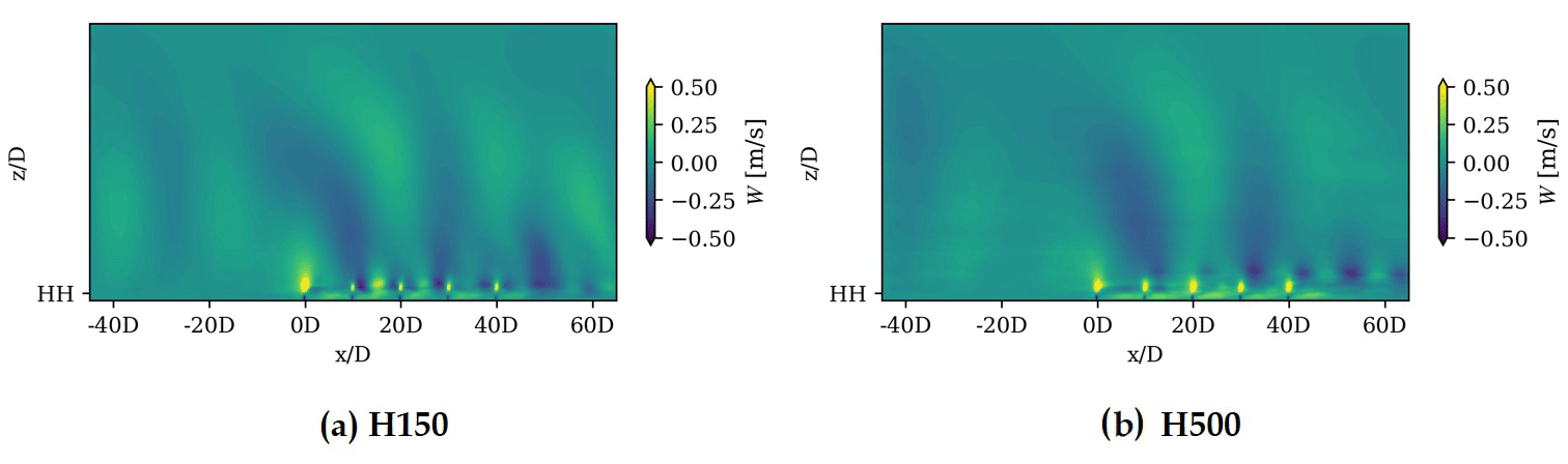
Figure 18 Time-averaged vertical velocity contour from UU SOWFA on the x–z plane through the sixth column turbine. The axes are normalized by rotor diameter, D, with 0D on the x axis indicating the location of the first-row turbines.

Thirdly, to examine the influence of BLH on wind farm operations, a neutral ABL with varying capping inversion heights was employed to minimize the influencing factors. However, BLH is governed by atmospheric stability and surface conditions, which can lead to considerable variations in atmospheric turbulence. Low BLHs are generally associated with a stably stratified ABL characterized by weaker turbulence, whereas an unstable ABL tends to have enhanced vertical mixing. Consequently, the findings of this study do not fully capture the complexities of the BLH's impact. Variations in turbulence levels across different BLHs may influence wake recovery within and behind a wind farm, thereby affecting overall performance.

In this study, different levels of modeling fidelity have been used with different numerical approaches. The overall results show good agreement. However, one cannot conclude that the results of farm efficiency are independent of the fidelity level. In this study, we do not investigate details on momentum entrainment, where one could expect the different fidelity levels to show differences. However, when assessing the overall efficiency under these specific conditions using the best practice in setup, the different fidelity models agree well considering trends but with quantitative differences.

Lastly, while all solvers in this comparison exhibit overall similar trends on wind farm performance and efficiency in various BLH scenarios, there is a lack of field observations to validate these large-wind-farm simulation results. We would also like to clarify here that the levels of efficiency presented here correspond to a few specific cases with an undisturbed wind speed close to rated, a relatively dense farm, and one wind direction aligned with the staggered layout. Therefore, the level of efficiency presented here for these cases should not be considered representative of general wind farm efficiency. To make that assessment, one needs to run a large set of simulations and weight them to climatology at specific sites.

5 Conclusions

This study investigates the impact of atmospheric boundary layer (ABL) height on the performance of gigawatt-scale wind farms. Through numerical simulations using multiple CFD solvers, the effects of ABL height and capping inversion on wind farm power generation, efficiency, and flow dynamics were analyzed.

The results indicate that a lower ABL height (for example, 150 m) leads to greater blockage and wake interaction effects, that is, reduced farm efficiency and higher energy losses, compared to deeper boundary layers (for example, 500 m). Furthermore, the thickness of the capping inversion layer was found to influence the wake recovery behind the wind farm.

The numerical simulations conducted by various research institutions and industry partners showed consistent overall trends, though significant variations were observed depending on the computational methods and domain size. The simulation cases performed are complex, and the results of the different methods show a variation of up to 10 %, with further research needed to limit this gap. Based on these results, it is not clear to what extent the variation depends on the fidelity level of the models used.

In summary, the study confirms that a deeper ABL generally improves the efficiency of wind farms and reduces energy losses due to blockage effects. The findings emphasize the importance of incorporating the height and stability of the ABL in wind energy models to improve the accuracy of the power generation predictions.

Appendix A: Single-turbine simulation output

Table A1 H150.

Table A2 H500.

Table A3 H500-dh500.

Appendix B: Wind farm flows on x–z and y–z planes

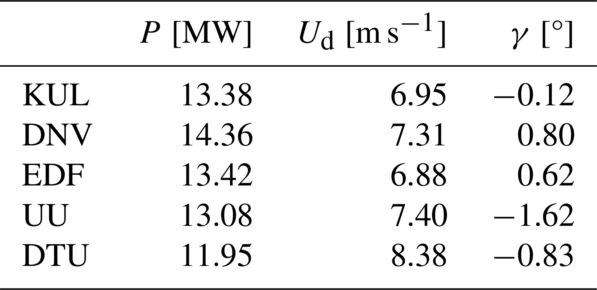
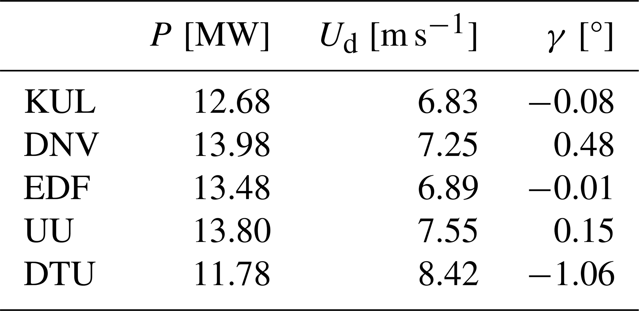
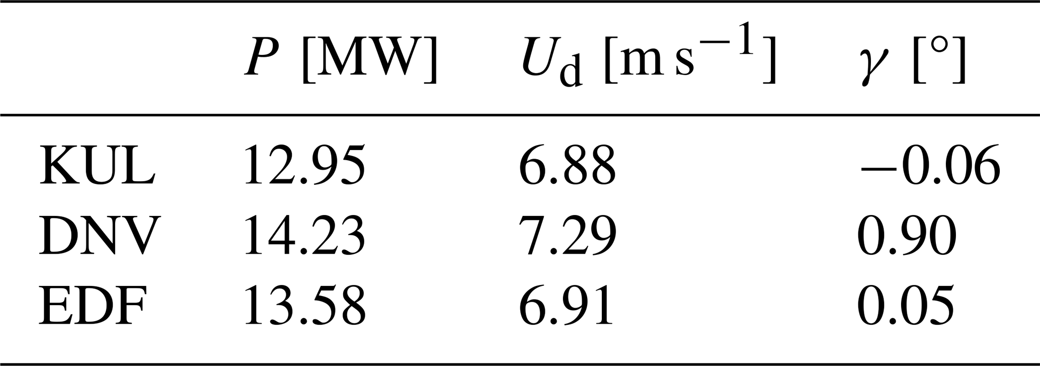
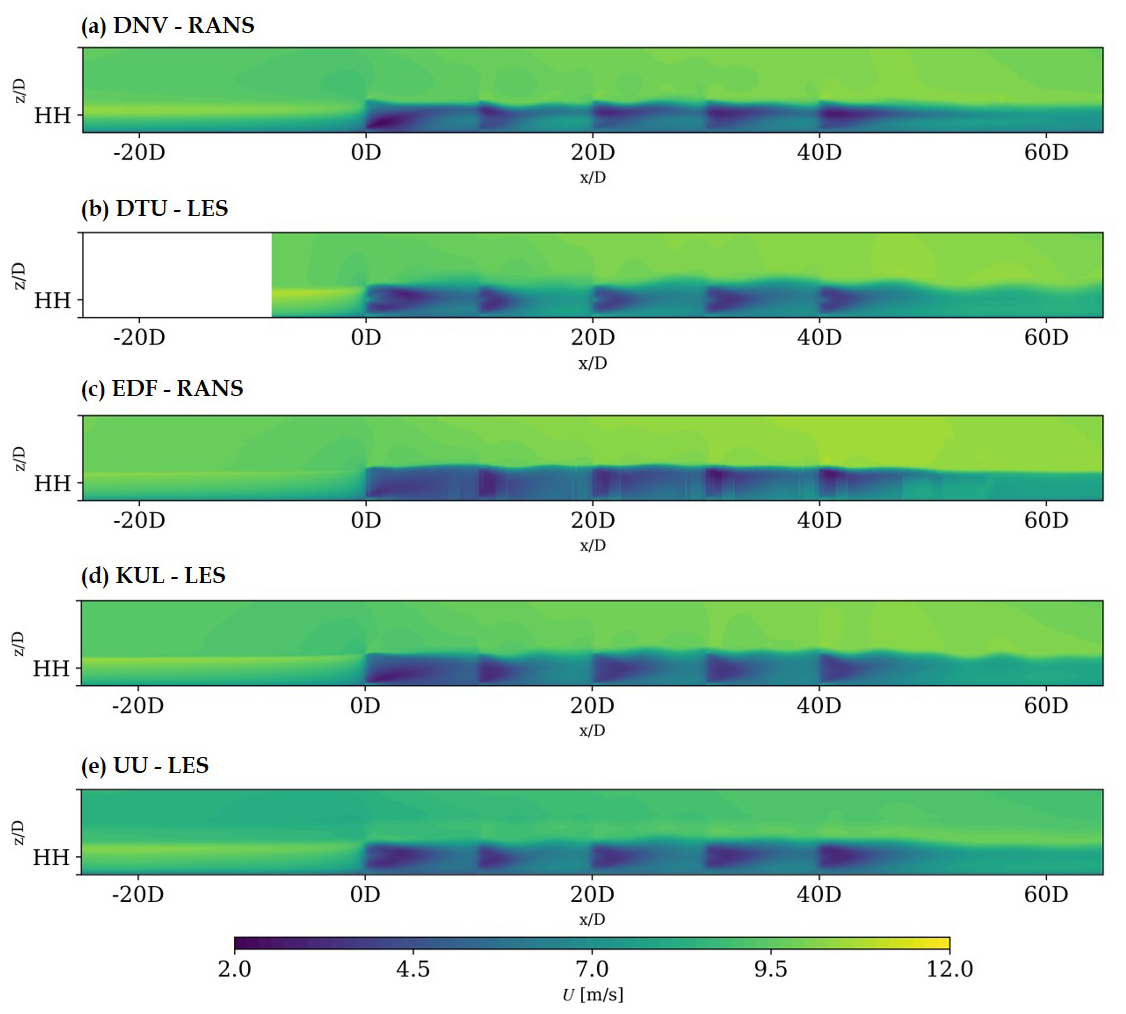
Figure B1 Mean streamwise velocity on the X–Z plane at the sixth column turbine for the H150 case.

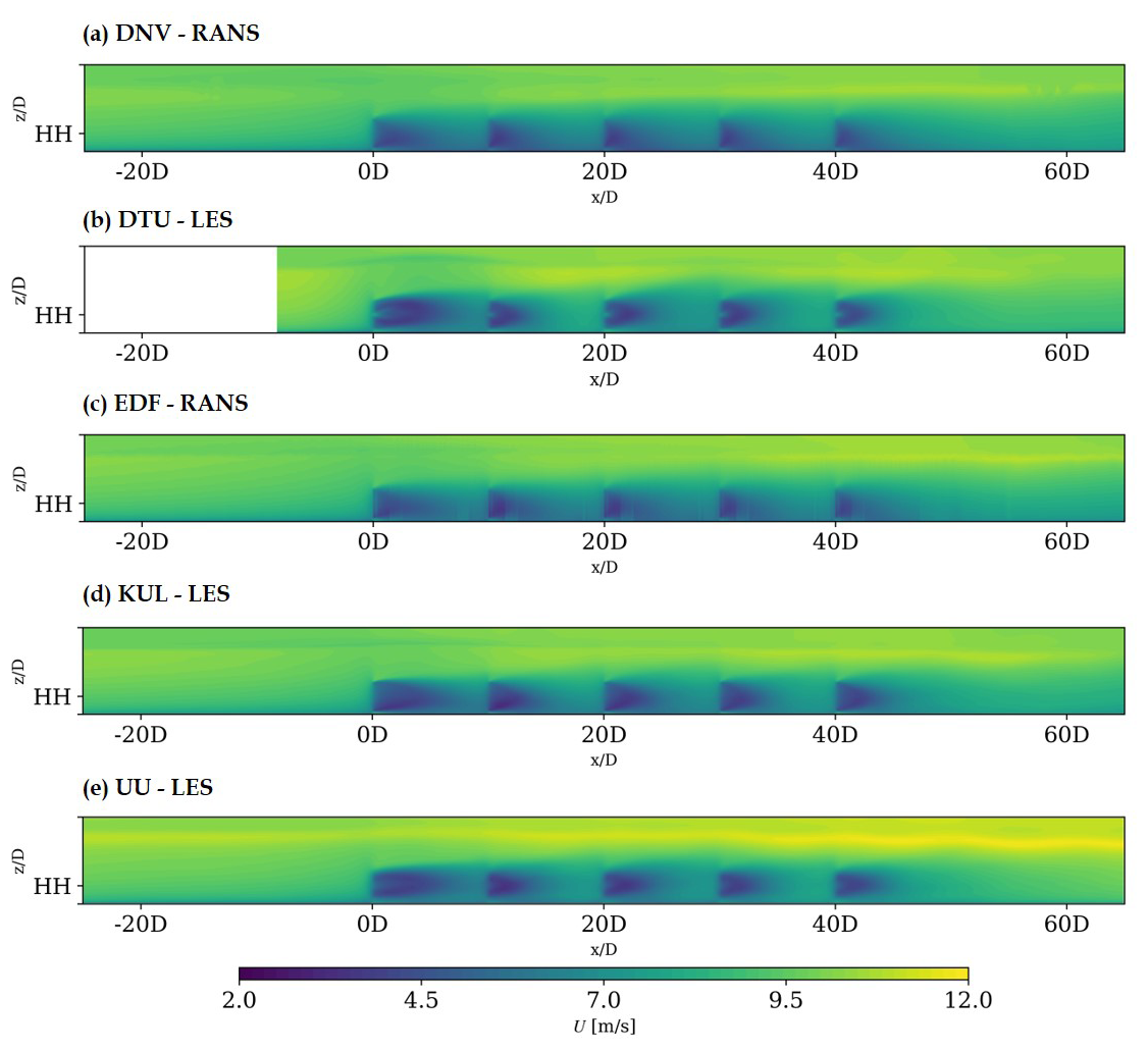
Figure B2 Mean streamwise velocity on the X–Z plane at the sixth column turbine for the H500 case.

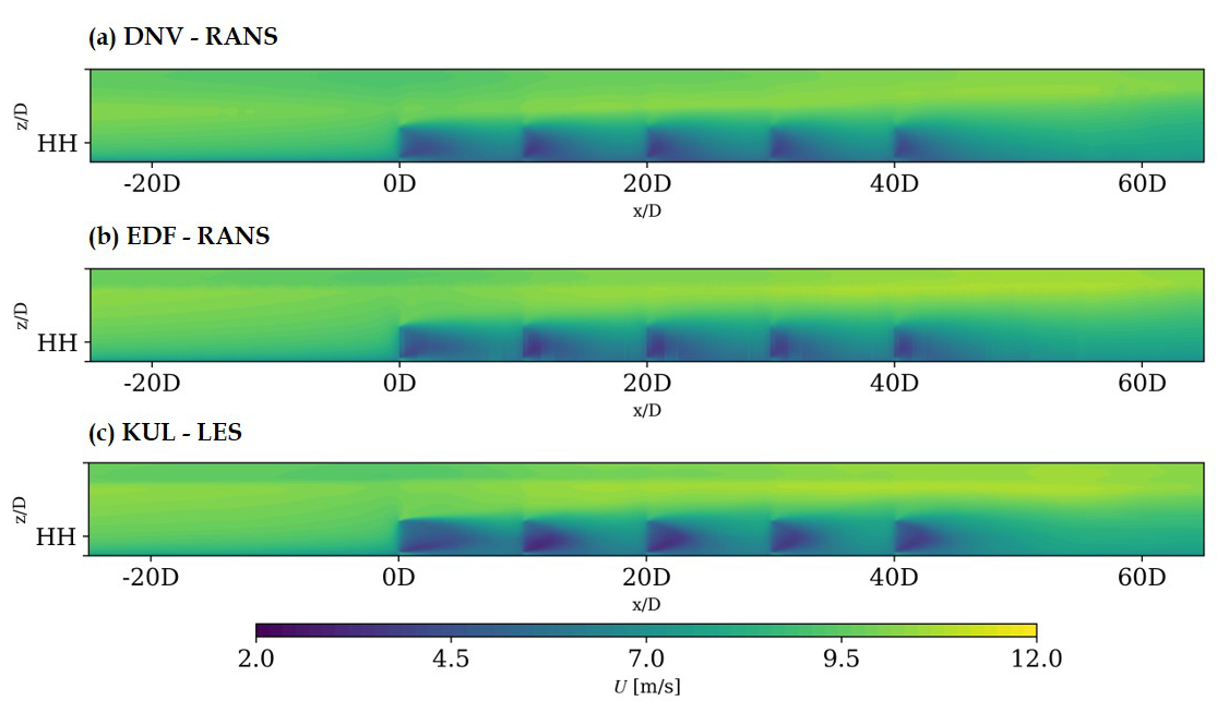
Figure B3 Mean streamwise velocity on the X–Z plane at the sixth column turbine for the H500-dh500 case.

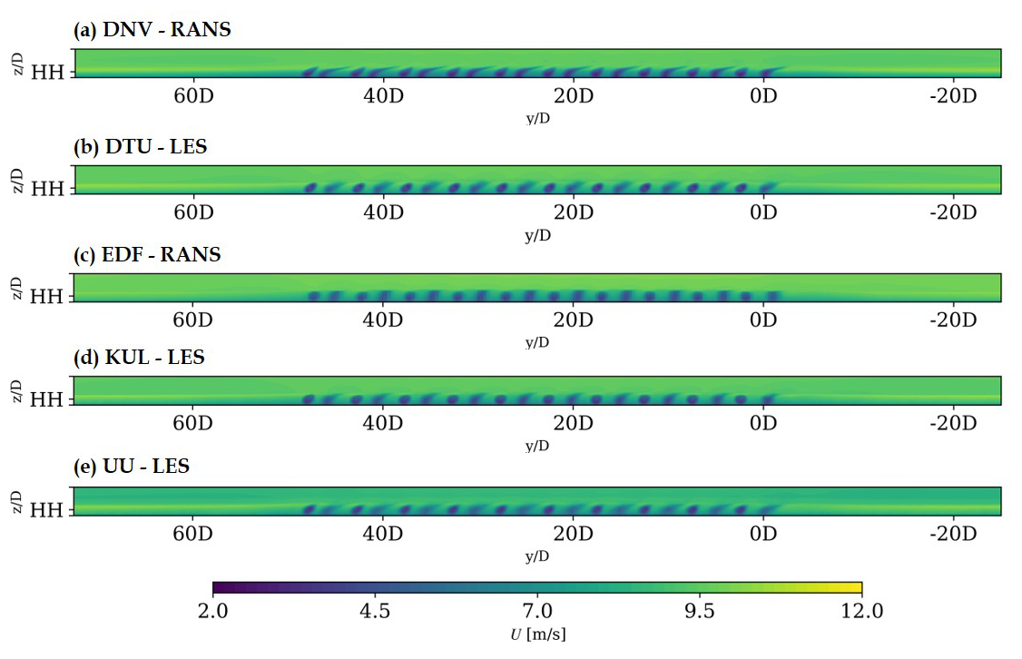
Figure B4 Mean streamwise velocity on the Y–Z plane 7.5D downstream of the first row for the H150 case, viewed from downstream.

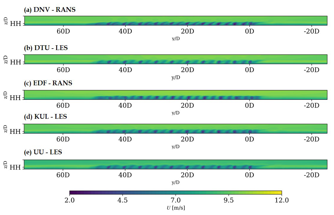
Figure B5 Mean streamwise velocity on the Y–Z plane 22.5D downstream of the first row for the H150 case, viewed from downstream.

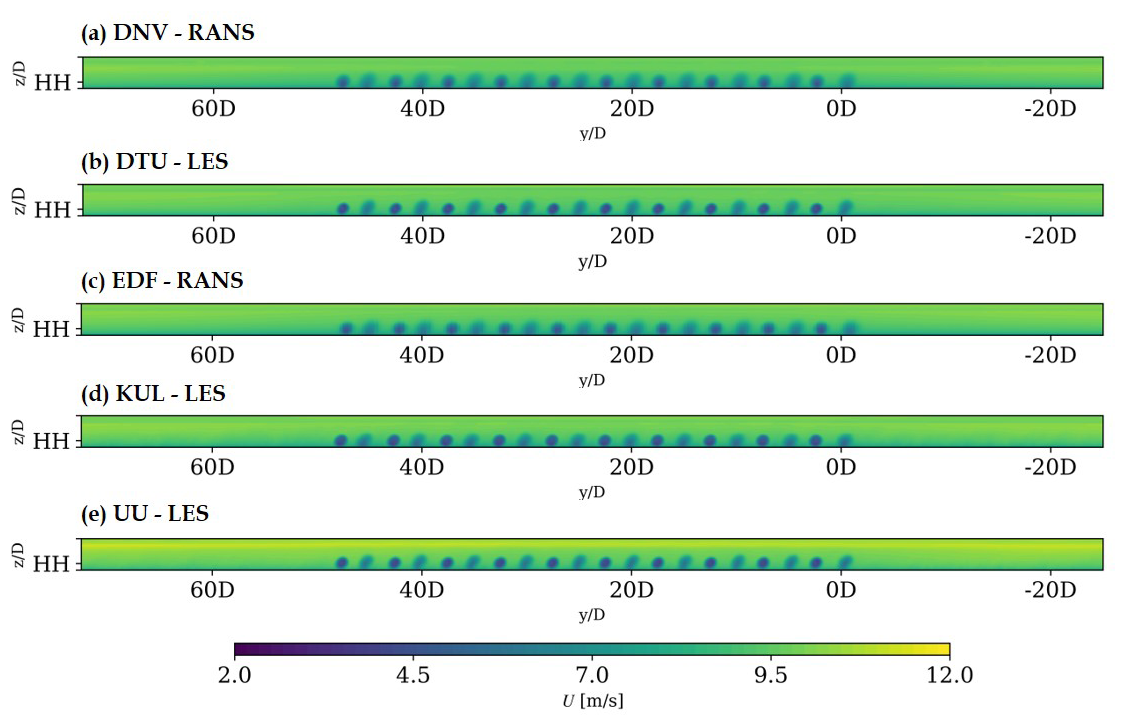
Figure B6 Mean streamwise velocity on the Y–Z plane 7.5D downstream of the first row for the H500 case, viewed from downstream.

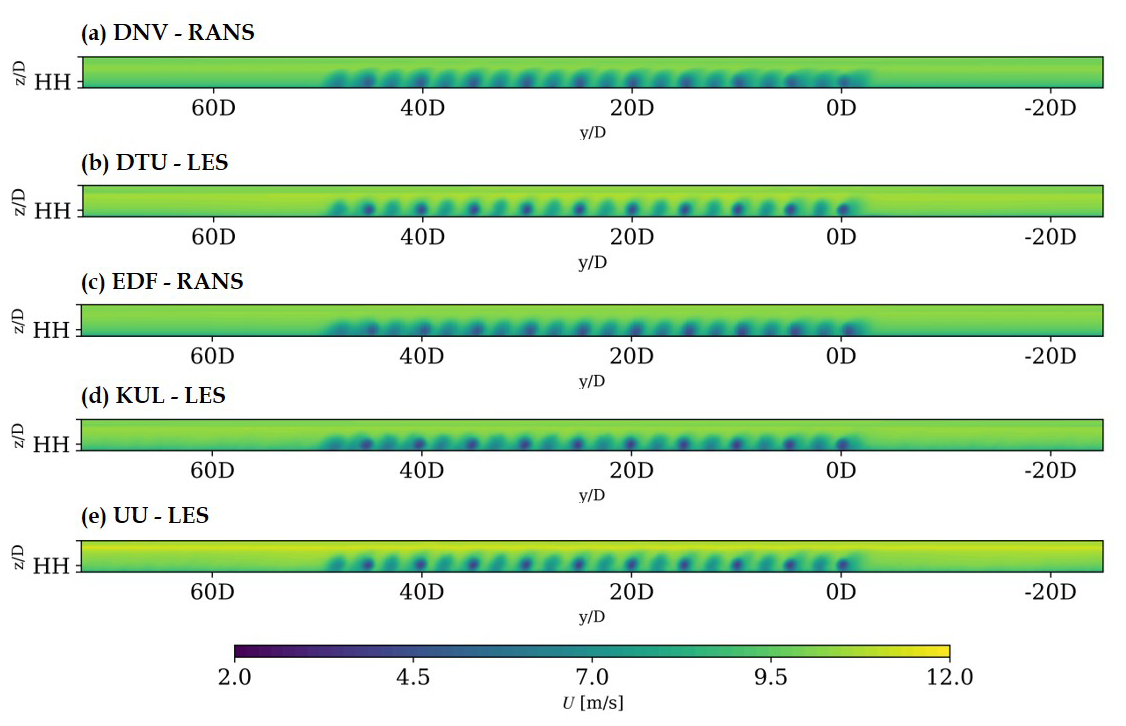
Figure B7 Mean streamwise velocity on the Y–Z plane 22.5D downstream of the first row for the H500 case, viewed from downstream.

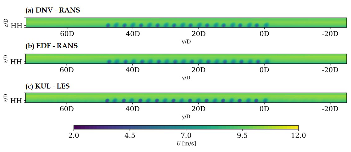
Figure B8 Mean streamwise velocity on the Y–Z plane 7.5D downstream of the first row for the H500-dh500 case, viewed from downstream.

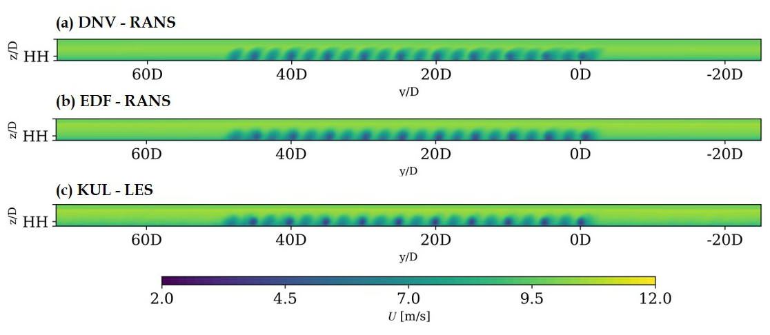
Figure B9 Mean streamwise velocity on the Y–Z plane 22.5D downstream of the first row for the H500-dh500 case, viewed from downstream.