How does turbulence change approaching a rotor?

For load calculations on wind turbines it is usually assumed that the turbulence approaching the rotor does not change its statistics as it goes through the induction zone. We investigate this assumption using a nacelle-mounted forward-looking pulsed lidar that measures low-frequency wind fluctuations simultaneously at distances between 0.5 and 3 rotor diameters upstream. The measurements show that below rated wind speed the low-frequency wind variance is reduced by up to 10 % at 0.5 rotor diameters upstream and above rated enhanced by up to 20 %. A quasi-steady model that takes into account the change in thrust coefficient with wind speed explains these variations partly. Large eddy simulations of turbulence approaching an actuator disk model of a rotor support the finding that the slope of the thrust curve influences the low-frequency fluctuations.

1 Introduction

It is routinely and often implicitly assumed in load calculations on wind turbines that the statistics of the turbulence do not change as the flow is approaching the rotor plane. As it is well known that the rotor affects the mean flow in front of the rotor it cannot be ruled out that the turbulence is also affected. In this paper we investigate this assumption experimentally with lidar measurements and large eddy simulation and compare the results with a simple model. We focus on low-frequency wind speed fluctuations.

Branlard et al. (2016) use vortex particle methods to calculate the effect of the turbine rotor on the incoming turbulence. They calculate the turbulent spectra at several center-line positions upstream of a Nordtank 500 kW wind turbine assuming a fixed thrust coefficient. They conclude that the presence of the rotor does not affect the turbulence spectrum significantly. However, at higher frequencies above 0.1 Hz, they observe a slight decrease in the power spectral density when the presence of the rotor is taken into account, implying marginally lower loads. They see no changes at lower frequencies. Branlard et al. (2016) emphasize that further investigations are necessary to conclude whether the effects of the stagnation on the turbulence are systematic or not (Branlard, 2017).

Simley et al. (2016) measure the turbulent inflow towards a Vestas V27 wind turbine using three synchronized continuous wave, scanning Doppler lidars. They clearly see the stagnation in front of the rotor. The standard deviation of the along-wind velocity component σ_u decreases slightly close to the rotor plane and they hypothesize that this is linked to the reduced mean velocity, which also affects the low-frequency fluctuations. They do not support this suggestion with spectral analysis and they also point out that the amount of data is limited. An additional complication is that the Doppler lidars average the turbulent flow field in ways that depend on the direction from the lidars to the measurement volumes and their distances.

The change in the turbulence spectrum due to the stagnation in front of the rotor is investigated theoretically using rapid distortion theory by Graham (2017). In a first step, he assumes that the turbulent scales are much smaller than the size of the rotor. He also assumes that the mean flow around the rotor is described by the model of Conway (1995), a linearized actuator disk model, and that the approaching turbulence is isotropic and described by the von Kármán spectrum. With these assumptions, he derives that ${\mathit{\sigma }}_u^{\mathrm{2}}/{\mathit{\sigma }}_{u\mathrm{\infty }}^{\mathrm{2}}$ increases with the induction factor a of the rotor, reaching a value of ${\mathit{\sigma }}_u^{\mathrm{2}}/{\mathit{\sigma }}_{u\mathrm{\infty }}^{\mathrm{2}}\approx \mathrm{1.34}$ at the induction factor of maximal energy extraction $a=\mathrm{1}/\mathrm{3}$. Here, ${\mathit{\sigma }}_{u\mathrm{\infty }}^{\mathrm{2}}$ is the undisturbed, upstream variance of the longitudinal wind speed component u and ${\mathit{\sigma }}_u^{\mathrm{2}}$ is the local variance. He analytically derives that the amplification of turbulence is not equally distributed on frequencies but rather concentrated at lower frequencies, leaving the inertial subrange almost unchanged. He also derives that the integral length scale of u in the y or z direction (i.e., perpendicular to the mean flow), which indicates how correlated fluctuations are across the rotor, increases as the flow approaches the rotor. The increase is a little less than the stretching by the mean flow in these perpendicular directions. Graham (2017) extends the theory to the more realistic case in which the integral length scale of the turbulence is not much smaller than the rotor by concentrating on the flow along the symmetry line of the rotor. The amplification of ${\mathit{\sigma }}_u^{\mathrm{2}}$ is less for the small length scale case than cases with turbulence length scales of the order of or larger than the rotor. The amplification of ${\mathit{\sigma }}_u^{\mathrm{2}}/{\mathit{\sigma }}_{u\mathrm{\infty }}^{\mathrm{2}}$ decreases from 24 to 7 % for $a=\mathrm{1}/\mathrm{3}$ as 2L_u∕D increases from 1 to 10, where L_u is the undisturbed integral length scale of u in the flow direction and D the rotor diameter. The variance slowly and asymptotically approaches its upstream value as $L_u/D\to \mathrm{\infty }$.

Farr and Hancock (2014) perform wind tunnel model studies of the flow upstream of a rotor. They find very little change in σ_u approaching the rotor, much less than expected from the small-scale rapid distortion limit discussed above. They suggest that the stagnation of the flow almost cancels out the amplification implied by rapid distortion theory.

In Sect. 2 we briefly discuss how quasi-steady fluctuations in the wind translate into fluctuations in the induction zone and we emphasize the effect of change in the induction with wind speed. That is followed by a discussion of a numerical experiment on turbulence in the induction zone in Sect. 3. Then we analyze a field experiment measuring low-frequency variations in the induction zone with a pulsed Doppler lidar (Sect. 4). Finally, results are presented and discussed in Sects. 5 and 6.

2 Theory

Low-frequency fluctuations are the focus of this paper and are discussed first. Then we summarize the results of Graham (2017), which should be valid for all frequencies but have a particularly simple solution for high frequencies. Finally, we discuss the limitation of rapid distortion theory for our particular application.

2.1 Quasi-steady fluctuations

Low-frequency or quasi-steady fluctuations are defined as variations in the wind speed U that are so slow that the rotor and the upstream flow have sufficient time to adjust to all the changes such that they appear as if the wind was steadily blowing at that wind speed. If $D=\mathrm{2}R=\mathrm{100}$ m and the induction zone extends 3D upstream then the low-frequency limit would be around f≈0.03 Hz for a free mean wind speed U_∞ of 10 m s⁻¹.

For a particular wind turbine, the mean wind speed on a line extending upstream from the center of the rotor depends on the ambient wind speed U_∞ and the distance from the rotor normalized by the rotor radius $\mathit{\xi }=x/R$ and is given by

$$\begin{array}{}\text{(1)}& f(\mathit{\xi },a,U_{\mathrm{\infty }})\equiv {\displaystyle \frac{U}{U_{\mathrm{\infty }}}}=\mathrm{1}-a\left(\mathrm{1}+{\displaystyle \frac{\mathit{\xi }}{\sqrt{\mathrm{1}+{\mathit{\xi }}^{\mathrm{2}}}}}\right).\end{array}$$

A slow fluctuation in the ambient wind speed U_∞ will produce slow variations in the wind speed in the induction zone U(x). The power spectral density at low frequencies is therefore amplified as

$$\begin{array}{}\text{(2)}& {\displaystyle \frac{S\left(x\right)}{S_{\mathrm{\infty }}}}={\left({\displaystyle \frac{\partial U}{\partial U_{\mathrm{\infty }}}}\right)}^{\mathrm{2}},\end{array}$$

where S(x) is the power spectral density (so the amplitude squared) at low frequencies at the position x and S_∞ is the upstream, undisturbed spectrum. The partial derivative can be expanded as follows:

$$\begin{array}{}\text{(3)}& {\displaystyle \frac{\partial U}{\partial U_{\mathrm{\infty }}}}={\displaystyle \frac{\partial f}{\partial U_{\mathrm{\infty }}}}{U}_{\mathrm{\infty }}+f=f-\left(\mathrm{1}+{\displaystyle \frac{\mathit{\xi }}{\sqrt{\mathrm{1}+{\mathit{\xi }}^{\mathrm{2}}}}}\right){\displaystyle \frac{\partial a}{\partial U_{\mathrm{\infty }}}}{U}_{\mathrm{\infty }}.\end{array}$$

Typically, a does not change for ambient wind speeds below rated wind speed, so the second term is negligible. The spectral amplification in Eq. (2) will then be proportional to the square of relative slowdown, which is of the order of but less than unity. Above rated, $\partial a/\partial U_{\mathrm{\infty }}$ will become negative and a positive amplification should be seen. A similar quasi-steady model for how low-frequency fluctuations of turbulence are modified by topography is presented by Mann (2000).

2.2 Small-scale fluctuations

Rapid distortion theory (RDT) for smaller turbulent scales corresponding to more rapid fluctuations is investigated by Batchelor and Proudman (1954) and Townsend (1976). Townsend calculates the response of initially isotropic turbulence to a contraction (or expansion) of the mean flow, which to some extent is what is happening in front of a rotor. The theory is used in Graham (2017) to produce amplifications of the velocity variance and the low-frequency part of the velocity spectrum shown in Fig. 1.

Figure 1 Amplification of the low-frequency spectrum and variance of longitudinal turbulence in the center of the rotor plane according to rapid distortion theory in the limit at which the length scale of the turbulence is much smaller than the rotor radius. The induction factor is $a=\mathrm{1}/\mathrm{3}$.

The theory assumes that the vorticity lines are advected by the mean flow and that the approaching turbulence is isotropic as described in the Introduction and by Conway (1995). The theory implies that the amplification is strongest at the lowest frequencies and almost absent at the highest frequencies. Their results in the limit of turbulent scales much smaller than the rotor diameter are shown in Fig. 1. In a wind tunnel contraction, the u component is diminished, also relative to the other components. In contrast, the u component is enhanced in the diverging flow in front of a rotor.

Now we analyze the applicability of RDT by estimating the relevant spatial and temporal scales. The term “rapid” in RDT means that the turbulent eddies should not be able to interact during the time it takes for the distortion of the flow to take place. The eddies should not “rotate” several times during the distortion phase; in other words, their lifetime τ should be longer than the distortion time 𝒯_D.

$$\begin{array}{}\text{(4)}& {\mathcal{T}}_D\ll \mathit{\tau }\end{array}$$

Another requirement for traditional RDT (Batchelor and Proudman, 1954; Townsend, 1976) but not for the work by Graham (2017) is that the shear or strain deforming the eddies is constant over the extent of the eddy. The strain changes appreciably in the wind turbine inflow zone over a length of the order of the size of the turbine, like its diameter D, so

$$\begin{array}{}\text{(5)}& D\ll k^{-\mathrm{1}},\end{array}$$

where we use the inverse wavenumber to characterize the size of the eddy. We now estimate the terms in Eqs. (4) and (5) to get a sense of the applicable frequency or wavenumber ranges of traditional RDT. We estimate the distortion timescale as ${\mathcal{T}}_D\approx D/U$, where U is the mean wind speed at hub height. In the work by Mann (1994) the simplest model for the eddy lifetime in the neutral atmospheric surface layer was

$$\begin{array}{}\text{(6)}& \mathit{\tau }=\mathrm{\Gamma }{\left({\displaystyle \frac{\mathrm{d}U}{\mathrm{d}z}}\right)}^{-\mathrm{1}}{\left(kL\right)}^{-\mathrm{2}/\mathrm{3}},\end{array}$$

where Γ is a constant of the order of 3, L is a length scale representative of the energy containing eddies, and dU∕dz the shear at hub height. The model implies that small eddies (large k) have a shorter lifetime than larger eddies, so it is in the limit of small eddies that RDT has a limitation. The same eddy lifetime model was use to extend the model by Mann (1994) to a semi-Lagrangian model (de Maré and Mann, 2016). For simplicity, we assume a logarithmic wind profile $U\left(z\right)=u_{\ast }/\mathit{\kappa }\log (z/z_{\mathrm{0}})$ (Wyngaard, 2010) so $\mathrm{d}U/\mathrm{d}z=u_{\ast }/\left(\mathit{\kappa }z\right)$ and that the diameter of the rotor is close to the hub height above the ground D≈z. Then, by isolating k in Eq. (4) we get

$$\begin{array}{}\text{(7)}& k\ll {\displaystyle \frac{{\left(\mathrm{\Gamma }\log (z/z_{\mathrm{0}})\right)}^{\mathrm{3}/\mathrm{2}}}{L}}\approx \mathrm{5}{\mathrm{m}}^{-\mathrm{1}},\end{array}$$

where we assume a hub height of z=80 m, a roughness length of z₀=0.05 m, and use IEC (2005) to get Γ=3.9 and L=33.6 m. This inequality states that only eddies smaller in scale than a meter or so will be short-lived enough not to feel the entire distortion in the induction zone. Equation (5) implies k≫0.013 m⁻¹, so looking at Fig. 4 we conclude that traditional RDT should be valid for frequencies higher than the peak of the spectrum (most energy containing eddies) and all the way up to the highest frequencies measured. Having estimated the range of applicability of traditional RDT we now turn our attention to an extension of RDT to larger scales.

The novelty of Graham (2017) is that he succeeds in calculating the velocity spectrum and variance without assuming that the length scale of the longitudinal turbulence L_u∞ is much smaller than the rotor. Graham develops the theory of Hunt (1973) further and cleverly exploits the axisymmetry of the mean flow to make the calculations feasible. As a function of L_u∞∕R, the low-frequency part of the velocity spectrum decays slowly to the ambient value after a small initial increase. This is in contrast to Eqs. (2) and (3), which predict a reduction of the velocity variance equal to f² for below rated where $\partial a/\partial U_{\mathrm{\infty }}=\mathrm{0}$. The cause of this difference is that Graham (2017) does not take into account the interaction of the vorticity lines with the actuator disk. The velocity field that a vorticity line induces will be nonzero at the rotor plane, particularly for turbulence scales larger than the rotor, and the actuator disk will reduce the fluctuation caused by this vorticity line near the rotor. The same is assumed in Lee (1989) on the axisymmetric expansion of turbulence because in that work there is no rotor to interact with after the expansion.

3 Numerical techniques

3.1 Wind turbine model

The wind turbine rotor is modeled as an actuator disk (AD) using the implementation proposed by Réthoré et al. (2014). Meyer Forsting et al. (2017) use the same model to simulate the induction zone of a 500 kW turbine and validated their predictions with lidar measurements.

The thrust force per unit area applied on the disk is assumed uniform and given by

$$\begin{array}{}\text{(8)}& {\displaystyle \frac{\mathrm{d}{F}_{\mathrm{T}}}{\mathrm{d}A}}={\displaystyle \frac{\mathrm{1}}{\mathrm{2}}}\mathit{\rho }{C}_{\mathrm{T}}\left(U_{\mathrm{\infty }}\right)U_{\mathrm{\infty }}^{\mathrm{2}},\end{array}$$

where ρ is the density of air and C_T(U_∞) is the thrust coefficient as a function of the free-stream velocity U_∞. The free-stream velocity is the velocity that would be at the disk location if the disk was not present. This velocity is not known a priori in an unsteady turbulent setting and therefore it is convenient to express the loading of the rotor in terms of the velocity averaged over the rotor disk, U_disk. For this reason we define a modified thrust coefficient, $C_{\mathrm{T}}^{*}\left(U_{\text{disk}}\right)$, as a function of the disk-averaged velocity:

$$\begin{array}{}\text{(9)}& C_{\mathrm{T}}^{*}\left(U_{\text{disk}}\right)=C_{\mathrm{T}}\left(U_{\mathrm{\infty }}\right){\displaystyle \frac{U_{\mathrm{\infty }}^{\mathrm{2}}}{U_{\text{disk}}^{\mathrm{2}}}}\end{array}$$

such that Eq. (8) becomes

$$\begin{array}{}\text{(10)}& {\displaystyle \frac{\mathrm{d}{F}_{\mathrm{T}}}{\mathrm{d}A}}={\displaystyle \frac{\mathrm{1}}{\mathrm{2}}}\mathit{\rho }{C}_{\mathrm{T}}^{*}\left(U_{\text{disk}}\right)U_{\text{disk}}^{\mathrm{2}}.\end{array}$$

The C_T curve used in the present AD simulations is obtained from steady-state simulations of the Siemens turbine presented by Troldborg and Meyer Forsting (2017) with a rated power of 2.3 MW at 11.5 m s⁻¹. From their simulations, we also extract the relation between U_∞ and U_disk and thereby the $C_{\mathrm{T}}^{*}$ curve. Figure 2 shows the variation in C_T and $C_{\mathrm{T}}^{*}$ with respect to U_∞ and U_disk, respectively. As expected $C_{\mathrm{T}}^{*}$ reaches greater levels than C_T because U_disk is lower than U_∞.

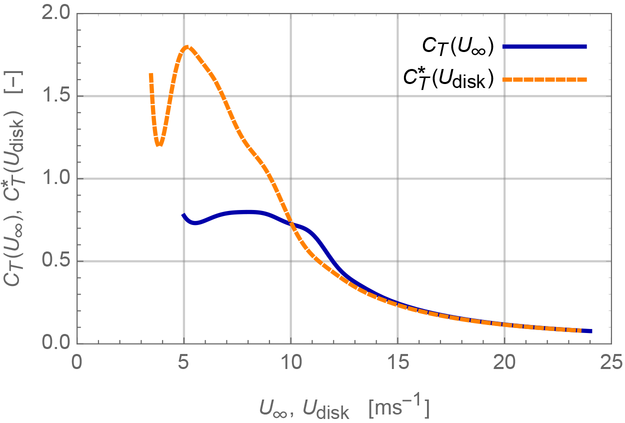
Figure 2 Thrust coefficient C_T and modified thrust coefficient $C_{\mathrm{T}}^{*}$ as functions of U_∞ and U_disk, respectively.

The loading and power of the real Siemens turbine is controlled by regulating the rotational speed and pitch of the blades. The control essentially depends on the local flow conditions at the rotor disk. Thus, using U_disk to determine the load level at each instant in time is a simple method for mimicking the behavior of the controller.

3.2 Computational domain

The computational domain is Cartesian and has dimensions $(L_x,L_y,L_z)=(\mathrm{40}R,\mathrm{25}R,\mathrm{25}R)$, where L_x, L_y, and L_z are the domain length, width, and height, respectively, and R=46.3 m. The rotor is located in the center of the domain, i.e., $(x,y,z)=(\mathrm{20}R,\mathrm{12.5}R,\mathrm{12.5}R)$ with its center axis aligned with the x direction (flow direction). The number of grid points in each direction of the domain is $(N_x,N_y,N_z)=(\mathrm{320},\mathrm{128},\mathrm{128})$. In the region defined by $\mathrm{8.5}R\le x\le \mathrm{21.5}R$, $\mathrm{11.05}R\le y\le \mathrm{13.95}R$, and $\mathrm{11.05}R\le z\le \mathrm{13.95}R$, the grid cells are cubic with a side length of R∕27.5. The reason for concentrating cells in this part of the domain is to better resolve the turbulent fluctuations in the region upstream of the rotor. Outside of this region, the cells are stretched towards the outer boundaries.

The boundary conditions are as follows: a fixed uniform velocity is prescribed at the inlet (x=0), bottom (z=0), and top (z=25R) boundaries. Periodic conditions are applied at the sides (y=0 and y=25R) and a zero-gradient Neumann condition is applied to the velocity at the outlet (z=40R).

3.3 Turbulent inflow

The turbulent inflow is generated using the model of Mann (1994). The three parameters governing the Mann spectral tensor model are selected according to the findings of Peña et al. (2017) and represent the best fit to the measured conditions at Nørrekær Enge, which is the site of the lidar turbulence measurements. The output of the Mann simulation algorithm (Mann, 1998) is a spatial box of turbulent fluctuations, which are converted to time domain via Taylor's frozen turbulence hypothesis. The dimensions of the generated box are $(L_X,L_Y,L_Z)=(\mathrm{512}R,\mathrm{16}R,\mathrm{16}R)$, with a resolution of $\mathrm{\Delta }=R/\mathrm{8}$.

The turbulent fluctuations are introduced into the computational domain in a cross section located 8.25R upstream of the rotor using the technique described by Troldborg et al. (2014). Note that only one-quarter of the full cross-flow extent of the box is introduced in the simulations in order to avoid any influence of periodicity in the turbulence.

3.4 Flow solver and simulation setup

The simulations are carried out using the incompressible Navier–Stokes flow solver EllipSys3D (Michelsen, 1992, 1994; Sørensen, 1995). EllipSys3D solves the finite-volume discretized equations in general curvilinear coordinates utilizing a collocated grid arrangement. The code uses a modified Rhie–Chow algorithm (Réthoré and Sørensen, 2012; Troldborg et al., 2015) to avoid pressure velocity decoupling. The simulations are carried out as detached eddy simulations (DESs) using the k−ω SST (shear stress transport) model by Strelets (2001). The convective terms are discretized using a hybrid scheme, which switches between the Quadratic Upstream Interpolation for Convective Kinematics (QUICK) scheme (Leonard, 1979) in the Reynolds-averaged Navier–Stokes (RANS) regions and a fourth-order central difference scheme in the large eddy simulation (LES) regions. The switching is determined through a limiter function given by Strelets (2001). The coupled momentum and pressure-correction equations are solved using the Semi-Implicit Method for Pressure Linked Equations (SIMPLE) algorithm (Patankar and Spalding, 1972). The solution is advanced in time using a second-order iterative time-stepping method using a time step of Δt=0.08 s. Simulations are carried out at free-stream velocities of U_∞=7, 8, 9, 11, and 13 m s⁻¹ in order to cover operations both below and above rated wind speed. In addition, we also do a simulation at 11.5 m s⁻¹ where the amplification of the low-frequency fluctuations should peak. Simulations are conducted both with and without a turbine included in the domain such that a one-to-one map in both space and time can be made of the influence of the rotor induction zone on the turbulence. The benefit of this approach is that it is insensitive to the distortion of the inserted turbulence, which is known to occur when the fluctuations are not in balance with the flow in which they are inserted.

4 Lidar experiment

The experiment took place at a 13-wind-turbine farm in northern Denmark in generally flat terrain. A five-beam pulsed prototype lidar from Avent was mounted on the nacelle of a Siemens 2.3MW wind turbine with a hub height of 81.8 and D=92.6 m. Only the central beam of the Avent lidar looking horizontally upstream of the turbine was used in this investigation. The lidar measured the line-of-sight velocity at 10 range gates centered at 49, 72, 95, 109, 121, 142, 165, 188, 235, and 281 m upstream of the rotor at a sampling frequency of 0.2 Hz. All details about the experiment may be found in Peña et al. (2017).

Figure 3 (a) U(x)∕U_∞ as a function of the upstream distance from the rotor averaged over different intervals of U_∞. The curves are fits to Eq. (1). (b) The induction factor a determined by fitting Eq. (1) to 10 min means of the lidar measurements. The black curve is based on interval medians.

5 Results

The line-of-sight velocity in the range gate centered around 235 m from the lidar and the wind speed from a WindSensor cup anemometer at the same distance and at hub height is compared to ensure the viability of the lidar. We find a slope deviating 1 % from 1 and a correlation coefficient of 0.98. The scatter is larger than other similar comparisons (Sathe et al., 2015). Due to the yawing of the turbine, the measurements are rarely collocated. An additional difference between the measurements is that the cup measures the “wind way” (Kristensen, 1999), while the lidar measures the component of the wind vector in the direction the wind turbine is pointing.

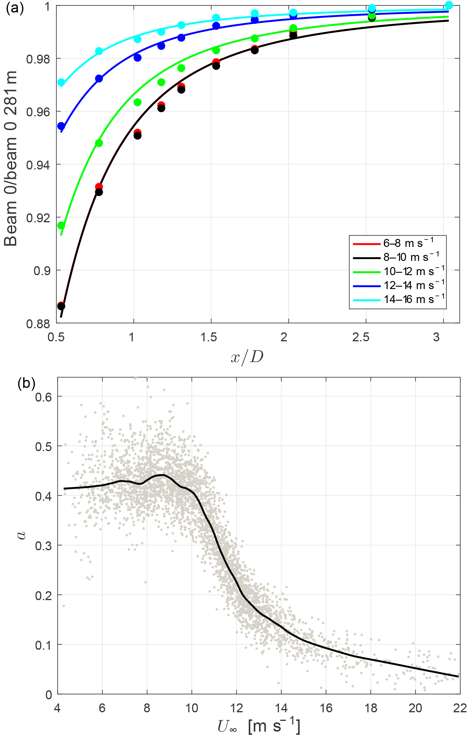
Having ensured the quality of the measurements we calculate the 10 min average of the u component of the wind and fit Eq. (1) to the measurements. That gives the value of a as a function of U_∞, which we assume is equal to the velocity measured at the furthest range gate. The induction factors from the undisturbed sector (Peña et al., 2017) are shown in Fig. 3b together with a smooth curve through the points, which is later used to compute $\partial a/\partial U_{\mathrm{\infty }}$. For wind speeds below rated the induction factor reaches levels above 0.4, which is higher than the expectation of approximately 0.3. The reason for this is that the quasi-steady model assumes a uniform load distribution and therefore tends to underestimate the induced velocity of real rotors, which have a nonuniform loading, as shown by Troldborg and Meyer Forsting (2017). For a given C_T, this bias causes an overestimation of the induction factor when the model is fitted to measurements of the upstream velocity. The bias is particularly dominant for the Siemens 2.3 MW because it has a high local loading below rated wind speed; see Troldborg and Meyer Forsting (2017). Figure 3a shows values of the measured u(x)∕U_∞ averaged in intervals of U_∞ with fits of Eq. (1) superimposed. It can be seen that the intervals below the rated wind speed $\mathrm{6}<U_{\mathrm{\infty }}<\mathrm{8}$ and $\mathrm{8}<U_{\mathrm{\infty }}<\mathrm{10}$ m s⁻¹ almost coincide.

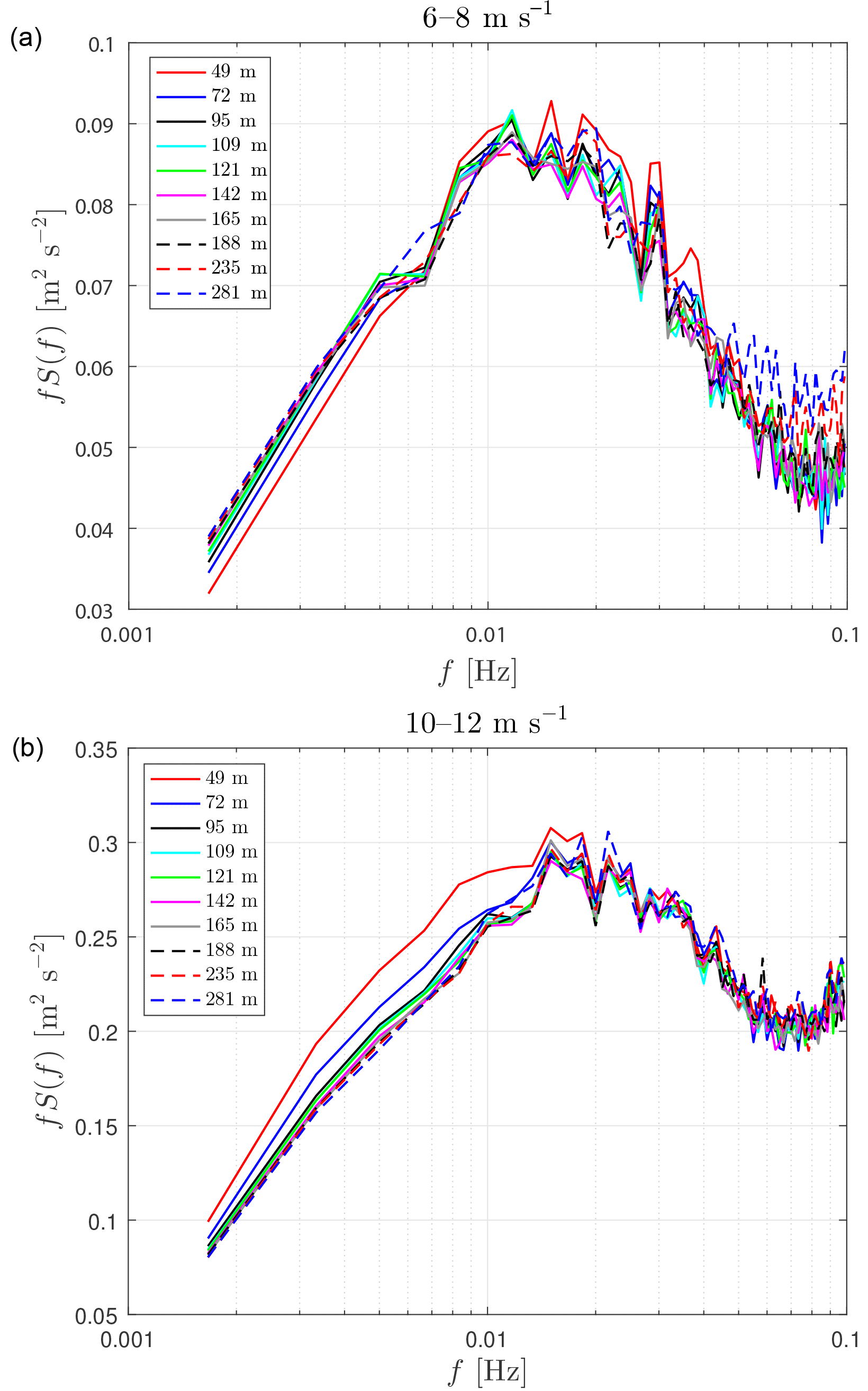
Figure 4 (a) Spectra of the line-of-sight velocity measured by the lidar as a function of upstream distance to the rotor averaged over all measurements with $\mathrm{6}<U_{\mathrm{\infty }}<\mathrm{8}$ m s⁻¹. (b) The same, but for $\mathrm{10}<U_{\mathrm{\infty }}<\mathrm{12}$ m s⁻¹.

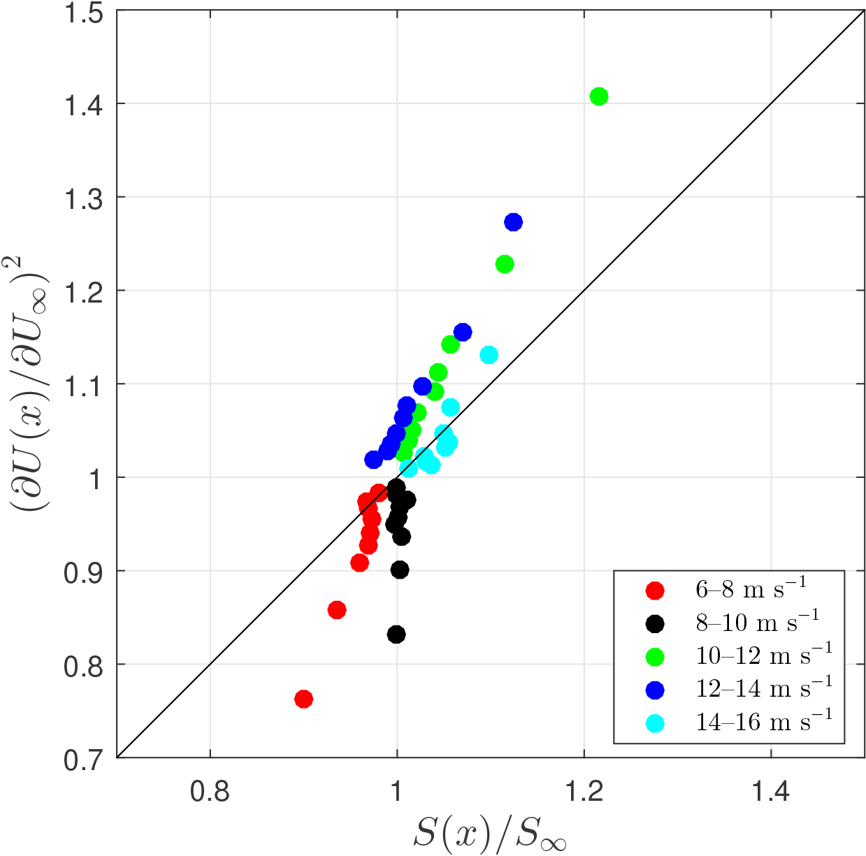
Figure 5 Change in low-frequency (f<0.007 Hz) spectral power of the longitudinal velocity component measured by the lidar compared to $(\partial U(x)/\partial U_{\mathrm{\infty }}{)}^{\mathrm{2}}$. The different points for a given wind speed interval correspond to different distances from the rotor x.

We now calculate the power spectrum of the velocity at each range gate in all 2 m s⁻¹ intervals of U_∞. These are based on 10 min time series so the lowest frequency investigated is $f=\mathrm{1}/\mathrm{600}\mathrm{Hz}=\mathrm{0.00167}$ Hz. Two examples are shown in Fig. 4 for U_∞ where a is constant with U_∞ and for a velocity where a rapidly decreases as a function of U_∞. For low frequencies, the power spectra for the low U_∞ coincide for most ranges except for those closest to the rotor when they are slightly but significantly lower. Conversely, for the higher U_∞, the spectra close to the rotor are significantly higher than the upstream spectra. The experiment has the great advantage that the measurements at all range gates are done simultaneously with the same instrument, making the detection of small differences possible.

The experimental results are summarized in Fig. 5. Here we calculate the low-frequency spectral amplification as measured by the lidar $S_{\text{low}}\left(x\right)/S_{\text{low},\mathrm{\infty }}$, where

$$\begin{array}{}\text{(11)}& S_{\text{low}}\equiv \underset{\mathrm{1}/\mathrm{600}\mathrm{Hz}}{\overset{\mathrm{4}/\mathrm{600}\mathrm{Hz}}{\int }}S\left(f\right)\mathrm{d}f;\end{array}$$

i.e., we add the four lowest-frequency bins of the 10 min average spectra. We calculate the low-frequency fluctuations using different upper frequency limits. The results vary but the trend remains. On the y axis, we plot the expected amplification according to the quasi-steady model in Eq. (3) for which the induction factor and its slope are derived from the solid curve in Fig. 3b. The cloud of points corresponding to each U_∞ bin represents results from nine range gates (the tenth is used for normalization assuming it is far enough away to represent the ambient flow). The trend that the low-frequency fluctuations are reduced below rated and amplified above is captured but the exact magnitude is not.

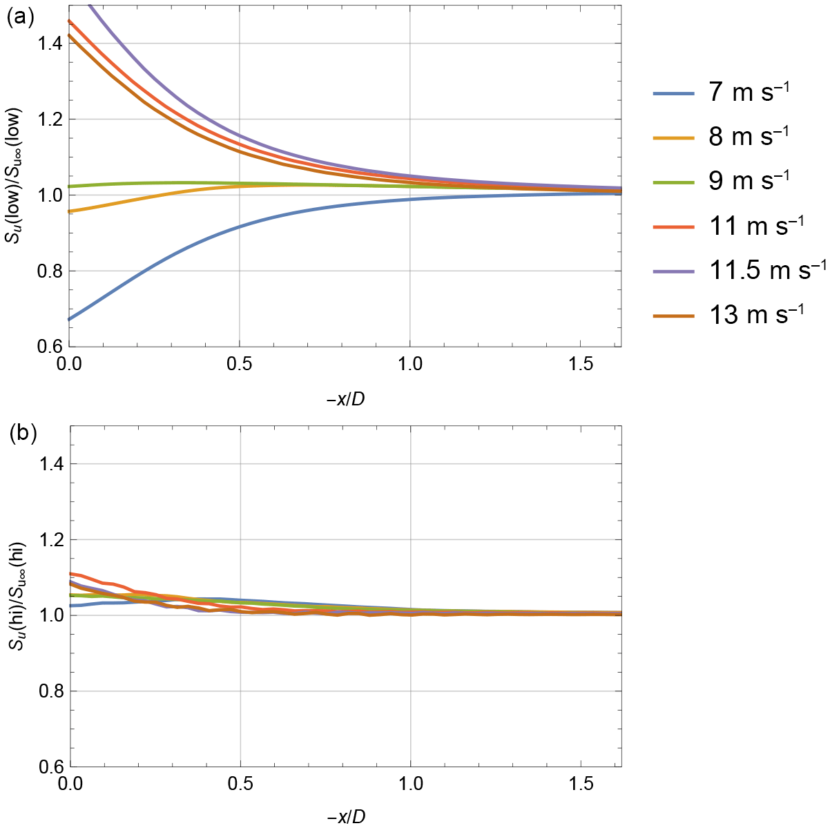
Figure 6 Low-frequency (f<0.03 Hz) and high-frequency (f>0.03 Hz) variances from LES in panels (a) and (b), respectively.

We now turn to the analysis of the LES simulations. Since the turbulence is not completely homogeneous in the stream-wise direction, we determine the effect of the rotor on the fluctuations at a position x by comparing the two simulations with and without the rotor at that position. In Fig. 6 we show the relative changes of turbulence divided into low and high frequencies. At low frequencies the fluctuations below rated wind speed are reduced while they are amplified above rated. The high-frequency fluctuations, or what the LES can resolve of them, change very little.

In Fig. 7 we summarize the results and compare them with the quasi-steady model. The theoretical prediction is based on the thrust curve shown in Fig. 2. We put a fifth-order spline through the points to be able to do derivatives and then we use the relation

$$\begin{array}{}\text{(12)}& a={\displaystyle \frac{\mathrm{1}}{\mathrm{2}}}\left(\mathrm{1}-\sqrt{\mathrm{1}-C_{\mathrm{T}}}\right)\end{array}$$

to get the induction factor (Hansen, 2015). We are then able to use Eq. (3) to predict the change in low-frequency fluctuations. We do that for two distances from the rotor, x=0 and $x=-R$. Again the model has the trends right, but the magnitude, especially below rated, is exaggerated.

Since the theory by Graham (2017) predicts an increase in low-frequency u fluctuations near the rotor, a combination of the two models could potentially improve the results.

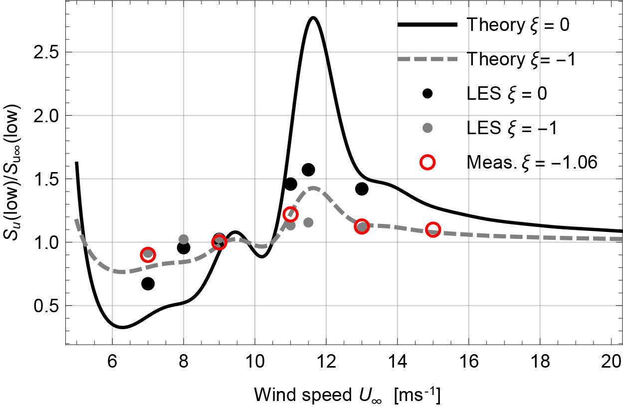
Figure 7 Change in low-frequency (f<0.03 Hz) spectral power of the longitudinal velocity component in the rotor plane and one radius upstream. The dots are the LES simulations, while the lines are the quasi-steady model based on Eqs. (2) and (3). The circles are lidar measurements using Eq. (11) at $\mathit{\xi }=-\mathrm{1.06}$.

6 Conclusions

The often used assumption that the statistics of turbulence approaching a wind turbine rotor are unaltered relative to its upstream values is investigated in this paper. Since the mean wind speed is reduced in the induction zone one cannot rule out the possibility that the turbulence is also affected.

A nacelle-mounted forward-looking pulsed lidar is used to measure low-frequency wind fluctuations upstream of a wind turbine rotor situated in flat, homogeneous terrain. It measures wind speeds simultaneously at 10 ranges between 0.5 and 3 rotor diameters upstream sampling at 0.2 Hz. The integral of the velocity spectrum up to a frequency of 1∕150 Hz is reduced by up to 10 % at 0.5 rotor diameters upstream and above rated enhanced by up to 20 %. The changes disappear rapidly further upstream.

A quasi-steady model that uses the C_T curve partly predicts the variation, but overestimates the changes. The model differs from a recent development in rapid distortion theory that is also applicable to low-frequency fluctuations (Graham, 2017).

An implementation of an actuator disk model in a large eddy simulation is used to investigate the changes in detail. The simulation is not completely homogeneous in the along-wind direction so the changes in turbulence statistics are found by comparing otherwise identical simulation runs with and without the rotor at corresponding positions. The simulations support the finding that the slope of the thrust curve influences the low-frequency fluctuations, but the simple quasi-steady model overestimates the changes. The exact consequences for loads are not investigated in this work.