Determination of optimal wind turbine alignment into the wind and detection of alignment changes with SCADA data

Upwind horizontal axis wind turbines need to be aligned with the main wind direction to maximize energy yield. Attempts have been made to improve the yaw alignment with advanced measurement equipment but most of these techniques introduce additional costs and rely on alignment tolerances with the rotor axis or the true north.

Turbines that are well aligned after commissioning may suffer an alignment degradation during their operational lifetime. Such changes need to be detected as soon as possible to minimize power losses. The objective of this paper is to propose a three-step methodology to improve turbine alignment and detect changes during operational lifetime with standard nacelle metrology (met) mast instruments (here: two cup anemometer and one wind vane).

In step one, a reference turbine and an external undisturbed reference wind signal, e.g., met mast or lidar are used to determine flow corrections for the nacelle wind direction instruments to obtain a turbine alignment with optimal power production. Secondly a nacelle wind speed correction enables the application of the previous step without additional external measurement equipment. Step three is a monitoring application and allows the detection of alignment changes on the wind direction measurement device by means of a flow equilibrium between the two anemometers behind the rotor.

The three steps are demonstrated at two 2 MW turbines together with a ground-based lidar. A first-order multilinear regression model gives sufficient correction of the flow distortion behind the rotor for our purposes and two wind vane alignment changes are detected with an accuracy of ±1.4^∘ within 3 days of operation after the change is introduced.

We show that standard turbine equipment is able to align a turbine with sufficient accuracy and changes to its alignment can be detected in a reasonably short time, which helps to minimize power losses.

1 Introduction

Modern large-utility-scale wind turbines are usually designed with an upwind rotor and therefore are active yaw controlled. The main reason for this design decision is the wind flow interference with the tower, which is less upwind of the structure. An active yaw control algorithm tries to align the rotor into the wind. The yaw system is slow compared to directional changes of the wind and immediate turbine reaction causes higher energy consumption of the yaw engines and wear of the components; therefore some degrees of yaw errors are accepted.

A systematic analysis of the impact of skewed flow on power production was set up by Madsen (2000). He compared field measurements of a 100 kW rotor with aeroelastic simulation using standard blade element momentum theory implemented in the HawC code and a new actuator disc model of the HawC-3D code. He found good agreements between the new 3-D model and the measurements. Pedersen et al. (2002) used the same data and explained the power loss following a squared-cosine relationship with increasing yaw error larger than 30^∘.

The rotor disc area perpendicular to the wind direction is reduced by the cosine of the inflow angle, which explains the squared-cosine relationship of the power loss for large angles. Likewise the wind speed component perpendicular to the rotor also decreases by a cosine relation, and with the wind speed having a cubic impact on power a cubic-cosine relationship is more dominant for smaller angles (Burton et al., 2001; Mamidipudi et al., 2011). In addition to power losses, yaw errors also increase turbine loads (Wan et al., 2015; Damiani et al., 2018).

Achieving a good alignment of the turbine with the wind direction is difficult for the following reasons. On standard turbines, wind speed and wind direction measurements take place behind the rotor. This leads to flow distortion caused by the rotor blades and the nacelle. To overcome this problem, several techniques to measure the free-stream wind in front of the turbine have been presented in different publications. The authors (Mamidipudi et al., 2011; Fleming et al., 2014; Scholbrock et al., 2015; Brown and Oldroyd, 2015) propose using an upwind-looking nacelle-mounted lidar. Pedersen et al. (2008, 2014, 2015) and Demurtas et al. (2016) present a method to measure the free wind speed, direction and turbulence intensity with three rotating sonic anemometers on the spinner nose. Bottasso and Riboldi (2014) estimate yaw misalignment and vertical shear from cyclic blade loads.

But for all these suggested methods new hardware is involved, causing additional financial investments. Lidar solutions need multiple beams to provide a wind vector because one beam can only measure the line of site information. All necessary laser beams need free-flow conditions, and a homogeneous flow assumption is usually made. One beam being in the wake of neighboring turbines and the other beams being in free flow leads to the wrong interpretation of the wind direction (Kapp, 2017). Furthermore, according to the findings of McKay et al. (2013), the yaw alignment behavior changes for turbines with wind vanes mounted on the nacelle metrological mast when operating in the wake of neighboring turbines.

Presuming that the nacelle-mounted measurement equipment is calibrated to ensure good alignment with the wind direction after commissioning or after a service interval, there are chances that the wind direction instrument is loosened, bent or warped over time and orientation drifts (Bromm et al., 2018).

Current methods to detect a change in the alignment of turbines are based on wind direction in situ comparison in case of redundancy of the device on the nacelle or by comparing wind direction measurements nearby (e.g., other turbines, met masts or lidars). The absolute wind directions of one or more wind vanes in the neighborhood are compared. This method works only if all true north alignments have been performed with high accuracy. Still there is a small risk of having the nacelle wind vane misalignment in the same magnitude but with different sign than the north misalignment; then both errors average out and the apparent wind direction will not be suspicious.

The purpose of this paper is to propose a new methodology to determine the best turbine alignment with standard nacelle-based equipment and monitor this alignment for the early detection of persistent yaw misalignment due to the vane falling out of calibration. We start with some basic information and definitions about wind turbine yaw systems and explain the experimental test setup and data handling in Sect. 2. In Sect. 3.1 we describe a methodology to improve the alignment of a reference wind turbine with an undisturbed reference wind speed measurement to obtain the maximum power production. In Sect. 3.2, we derive a model to correct the nacelle wind speed measurement behind the rotor in order to repeat the alignment improvement without an external wind measurement device (e.g., met mast or lidar). Section 3.3 describes a technique allowing standard turbine nacelle met mast equipment (e.g., two cup anemometers and one wind vane) to detect an alignment change of the wind direction measurement device during operation. Results and discussion of a demonstration case with a test wind turbine operating with different alignment offsets is provided in Sect. 4, followed by the conclusion in Sect. 5.

2 General description of turbine alignment and experimental setup

2.1 Yaw control

The true wind direction ϑ can be derived from the nacelle position ϕ and the relative wind direction on the nacelle, referred to as yaw error γ, with

$$\begin{array}{}\text{(1)}& \mathit{\vartheta }=\mathit{\varphi }+\mathit{\gamma }.\end{array}$$

The nacelle position ϕ is the angle between the rotor axis and the marking of the true north as displayed in Fig. 1a. Turbines are aligned to the true north after commissioning, but the equipment to measure the rotation of the nacelle is often not accurate enough and leads to a drift of the true north marking during operational lifetime (Bromm et al., 2018). In consequence, old turbines in the fleet may often not show a correct true wind direction since the wind direction is derived from the sum of the yaw position and the yaw error γ (Eq. 1). This is not a problem for the yaw controller using only relative wind direction but for reanalysis purposes or sector management these data need to be corrected.

A yaw controller needs to find a good balance between minimizing the average yaw error as soon as possible and staying within the design limits of the yaw component. To account for this, most controller algorithms can operate in different envelopes separated with a certain hysteresis. For instance, at lower wind speeds, at which in general higher turbulence intensities occur, larger yaw error angles are accepted for a longer period before the yaw system starts to move. At higher and more steady wind speeds, the accepted misalignments and periods are reduced to enable the turbine to react faster to wind direction changes. This behavior is site dependant and different settings for different locations can be favorable. With an increasing number of yaw position corrections and decreasing acceptance of yaw errors, the quality of the measured wind direction on the nacelle becomes more important.

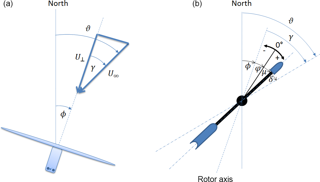
Figure 1 Definition of angles. (a) The angle between the rotor axis and the true north is called the nacelle position ϕ. The angle between the true wind direction (ϑ) U_∞ and its component perpendicular to the rotor plane U_⊥ is denoted as yaw error γ. (b) The wind vane is located behind the rotor. Its assembly angle φ with respect to the rotor axis, the measured value μ and the flow deflection angle δ between the wind vane and true wind direction sum up to the yaw error γ.

2.2 Wind direction measured by nacelle anemometry

Most wind turbines are equipped with one, or in case of the need for redundancy, a second wind direction measurement using a wind vane or sonic anemometer to measure the orientation of the rotor with regards to the incoming wind direction. In general the yaw controller is set up to adjust the nacelle direction towards a specific measured average value μ from the wind direction sensor. As the wind direction device is in the fixed reference system on the nacelle, the average of the measured value μ should converge to zero. In this way, negative values indicate inflow from the left (looking upwind) and positive values from the right. To ensure that the value 0^∘ is measured when the wind direction device is in line with the rotor axis, each instrument comes with a reference marking and needs to be properly aligned with the reference orientation of the nacelle. Some devices need to consider an assembly angle φ, when the measured value zero is not in line with the rotor axis. In our example in Fig. 1b, a good alignment is achieved for $\mathit{\phi }=\mathrm{0}{}^{\circ }$.

This task is challenging because manufacturing tolerances on the nacelle and its met tower can lead to some degrees of misalignment. Different optical techniques such as notch and bead sights or laser devices are used to measure the orientation of the instrument along the rotor axis of the turbine.

Figure 2 illustrates in a simplified manner how the flow behind a rotor is skewed as function of the aerodynamic thrust and torque and other disturbances attached to the nacelle roof. A wind direction measurement μ obtained from behind the rotor needs to be corrected with a flow deflection angle δ(U_∞Ω), which can be assumed constant or take into account its relationship of the wind speed U_∞ or rotor speed Ω (Kragh et al., 2013).

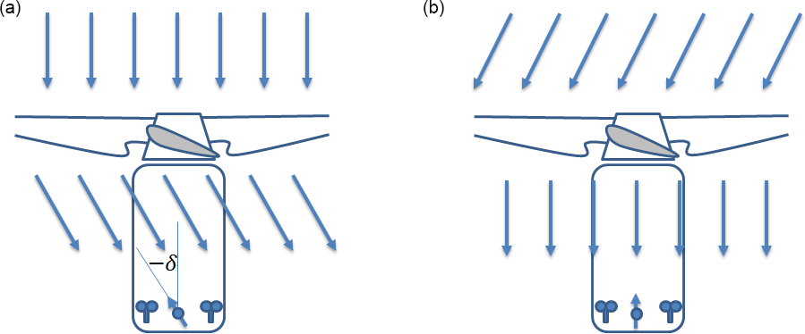
Figure 2 Illustration of the simplified flow in front of and behind the rotor. (a) The blade forces the flow to twist and an optimal aligned turbine obtains a flow deflection angle δ, which needs to be considered in the turbine alignment. (b) A turbine with the wind vane aligned to the rotor axis faces the wind at a certain yaw angle.

A well-aligned and flow-corrected wind direction measurement will then provide the measure of the yaw error with

$$\begin{array}{}\text{(2)}& \mathit{\gamma }=\mathit{\mu }+\mathit{\phi }+\mathit{\delta }\left(U_{\mathrm{\infty }}\mathrm{\Omega }\right),\end{array}$$

where μ is the output of the wind direction instrument, δ(U_∞Ω) the flow deflection function and φ the assembly angle. Because of the cyclical flow distortion of the rotating blades, the wind direction measurement μ fluctuates a lot and an averaging in the range of 10 s to 1 min is mandatory for the use of Eq. (2).

The yaw error vanishes if the flow is orientated perpendicular to the rotor plane since the flow deflection δ is compensated for by the well-aligned ($\mathit{\phi }=\mathrm{0}{}^{\circ }$) but skewed measurement μ. Negative γ values indicate flow from the left and positive values from the right. A positive flow deflection angle δ provokes the turbine to face more to the right when looking upwind.

A methodology to estimate the flow deflection function δ(U_∞Ω) based on a comparison between the true wind direction measurement at the turbine and a nearby met mast or lidar includes further stumbling caused by the accuracy of the true north alignment. An accurate true north alignment of a met mast wind direction instrument at hub height is difficult. The international standard for power curve verification testing based on nacelle anemometry (IEC 61400-12-2, 2013) provides a table with components of the combined uncertainty for a wind direction signal from the turbine and a met mast adding up to approximately ±6^∘.

Figure 3 shows an example of the yaw error γ plotted against the wind speed corrected with a constant flow deflection angle δ. The solid points with the black border represent wind speed bin medians and the solid line is the overall mean. In this example the median of the error varies depending on the mean wind speed between −4 and +2^∘. Thus, the assumption of a constant flow deflection angle δ has to accept a range of misalignments of at least ±3^∘. Kragh et al. (2013) suggest improving this behavior with a linear correction as a function of the rotor speed since the aerodynamic torque and the induced wake rotation are correlated with it.

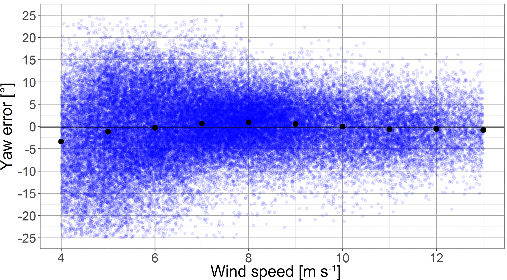
Figure 3 Turbine alignment check based on the comparison of a ground-based lidar wind direction measured with the velocity azimuth display (VAD) technique and the turbine wind direction (yaw error) plotted against the wind speed. The median yaw error per wind speed bin is indicated by the black dots and the overall mean by a horizontal line. Data are averages of 1 min periods and obtained from the experimental setup described in Sect. 2.3.

A simple method to correct the wind speed measurement on the nacelle, to be representative for the free-flow wind speed in front of the turbine, is a nacelle transfer function as described in IEC 61400-12-2 (2013). This linear model uses a slope β₁ and an offset β₀ in the form

$$\begin{array}{}\text{(3)}& v_{\mathrm{free}}=v_{\mathrm{nacelle}}{\mathit{\beta }}_{\mathrm{1}}+{\mathit{\beta }}_{\mathrm{0}}.\end{array}$$

Pedersen et al. (2013) introduce more advanced correction functions especially for spinner anemometry, including the induction factor as a function of the wind speed.

2.3 Experimental setup and data handling

A site with Senvion MM92 turbines (92 m rotor diameter, 2 MW rated power) has been chosen to validate the new alignment method. The two test turbines are installed on flat terrain in northeastern Germany. Figure 4 displays the layout of the test setup and a frequency distribution of the wind speed by wind direction of the recorded data. The turbines are 4.1 rotor diameters apart from each other approximately perpendicular to the prevailing wind direction. Meteorological data are recorded by a ground-based Leosphere Windcube V2 lidar as averages of 1 min periods in a distance between 2.5 and 3.1 rotor diameters. In addition to the standard supervisory control and data acquisition (SCADA) data with 10 min average periods, turbine data with a resolution of 1 Hz are available. Lidar and turbine data are synchronized with GPS time and merged as averages of 1 min periods. Downtimes and wind directions outside the free-flow sector are filtered but yaw activities during the 1 min period are neglected. The wind speed is corrected for air density as suggested in IEC 61400-12-1 (2017). Turbine WT1 has aerodynamically modified blades and is used to demonstrate the method of the alignment for best power production. To verify the monitoring ability of the method, two changes are made at Turbine WT2 with standard blades. At the first change the wind vane is mechanically aligned with notch and bead sights to ensure an assembly angle φ equal to zero and the flow deflection angle δ is set to 0^∘. The second change adds 7^∘ to the flow deflection angle δ for the rest of the test period.

Figure 4 Layout of the test wind farm and frequency distribution of wind speeds by wind direction. Two 2 MW turbines with a rotor diameter of 92 m turbines and a ground-based lidar measuring inflow conditions with the velocity azimuth display technique (VAD) in the free sector are shown.

2.4 Dynamic effects and time averaging

The standard wind turbine and environment condition data in the wind energy community are averages of 10 min periods. For the purpose of detecting the best operational orientation and to detect misalignments, it is beneficial to use a shorter averaging period. First, this gives more data points in total, and second, less averaging means less information gets lost.

In our demonstration in Sect. 4, we will use data averages of 1 min periods as lidar data of this sampling rate are available. Figure 5 provides the explanation why higher sampling rate improves the evaluation of the best turbine alignment. The blue dashed line is a density distribution of all available 10 min data samples as a function of the yaw error. The turbine controller will turn the nacelle towards 0^∘ when certain conditions are fulfilled. This leads to a high data density around 0^∘. High yaw errors (> 15^∘) are accepted from a load perspective for short periods only. Averages of 10 min periods may contain such events, but the mean value is closer to 0^∘. The effect of power loss for extreme yaw errors is much higher (red solid line: power loss as a function of the yaw error) and therefore it is beneficial to look at data with a higher sampling rate to better capture this effect.

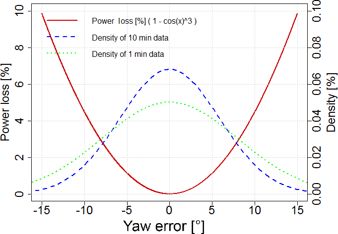
Figure 5 The red solid line indicates the power loss as a function of the yaw error, assuming the cubic-cosine relationship. The dotted and dashed lines represent data densities, fitted with Gaussian distributions. Both lines are based on the same raw data with 1 Hz resolution, but the green dotted distribution shows the data with an averaging period of 1 min and the blue dashed line is the data with 10 min averaging. Higher data resolution (e.g., 1 min data instead of 10 min data) has a larger standard deviation and therefore provides more data points at extreme conditions where the effects of power losses are more pronounced. This enables better evaluation of the best point of operation.

3 Method

There are now two variables which are key for a turbine with a wind direction device behind the rotor to operate at its optimum power production. First the flow deflection angle δ(U_∞,Ω) and second the assembly angle φ. The three steps in the following sections propose new methodologies to determine optimal values for these variables and a way to monitor and detect changes.

3.1 Best turbine alignment

The best turbine alignment maximizes power production. This is not automatically the case when the turbine faces orthogonal wind at hub height. The change of wind direction with height is called wind veer and leads to different angles of attack depending on the rotor angle of the blades. Our basic hypothesis to optimally align the turbine includes deriving the effective yaw error from a polynomial fit of the active power or the rotor speed as a function of the yaw error.

The active power measurement or respectively the rotor speed needs to be plotted against the yaw error γ (Fig. 6) for small wind speed bins. The power or respectively the rotor speed drops with increasing yaw error γ. A second-order polynomial fit with the method of least squares gives a convex curve. The orientation of the best production is revealed at its maximum. A deviation of the average yaw error from zero is used to correct the flow deflection angle for the corresponding wind speed bin (WSbin). Figure 6 also demonstrates the advantage of using data with a higher resolution than the standard 10 min SCADA data. Both data sets are simulated distributions of the variable of interest with a mean yaw error of 0^∘ and the standard deviations derived from Fig. 5. The simulation time is 1000 min. The 10 min averages (a) provoke less curvature at the polynomial fit, which may lead to small deviations in the mean yaw error interpretation. The higher data resolution (b) provides a more accurate result, closer to the simulated 0^∘ yaw error.

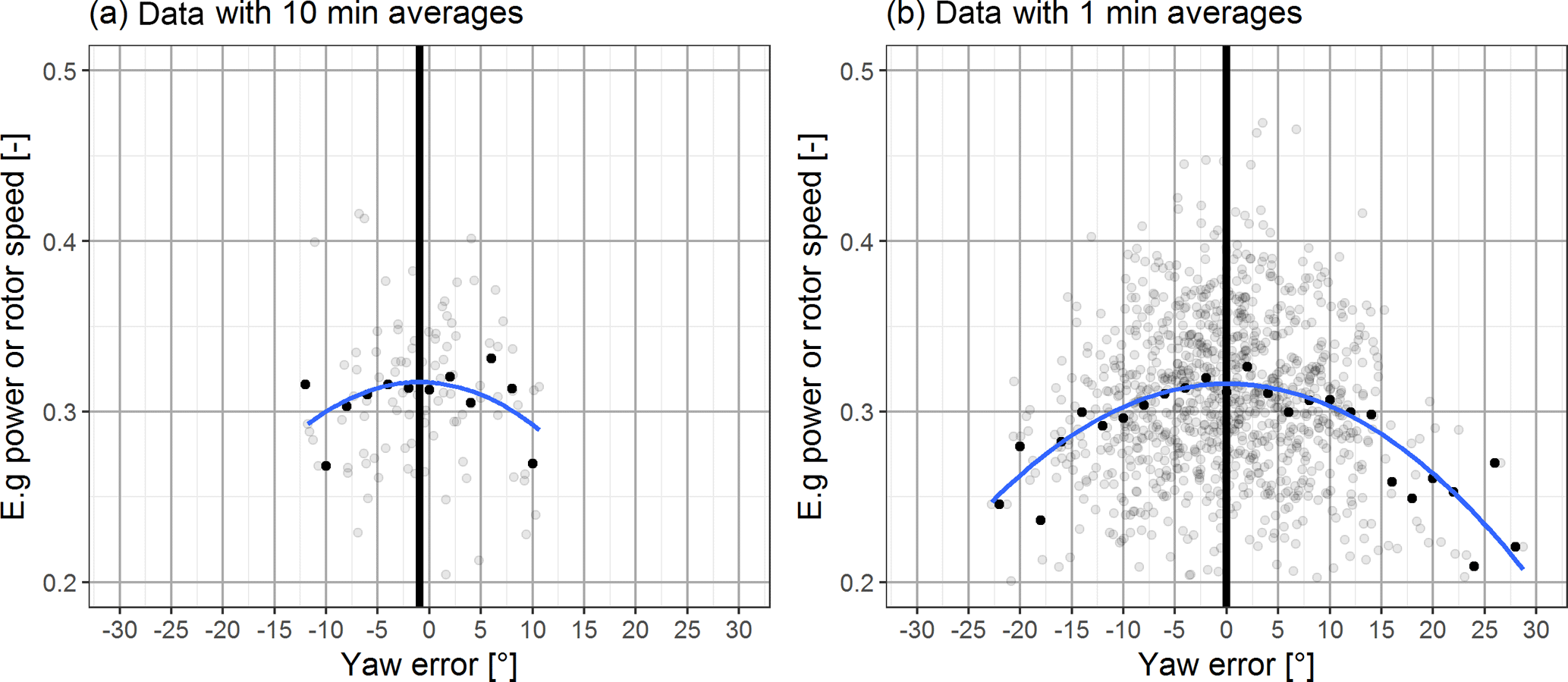
Figure 6 Example of the determination of the best operational alignment. The data are simulated with the same distribution derived from Fig. 5 with a mean yaw error of 0^∘ and 1000 min duration. Normalized active power or rotor speed for a specific wind speed bin as a function of the yaw error. The transparent dots are values with an averaging period of 1 min (b) and 10 min (a). The solid dots represent the yaw error bin averages. The curved line is a second-order polynomial fit with the method of least squares. The maximum is highlighted with a vertical bar. Data with averages of 10 min periods (a) show less curvature than data with 1 min (b), which can lead to small deviations for the derived mean yaw error.

For this technique, it is essential to have a high-quality reference of the wind speed. In the selected analysis sector, the wind speed measurement must not be influenced by the wind direction nor the way the turbine is aligned with the wind. This type of measurement can be obtained from a met mast or lidar in simple and flat terrain with no interference from neighboring turbines, which is ideally the case for prototype measurement.

3.2 Flow correction for nacelle instruments

The determination of the best turbine alignment, as described in the previous section, works only with a wind speed measurement which is not influenced by the yaw error itself. Therefore it is of great value to be able to correct the flow distortion at the nacelle instruments to avoid the necessity of additional external devices such as lidar, met mast or spinner anemometers.

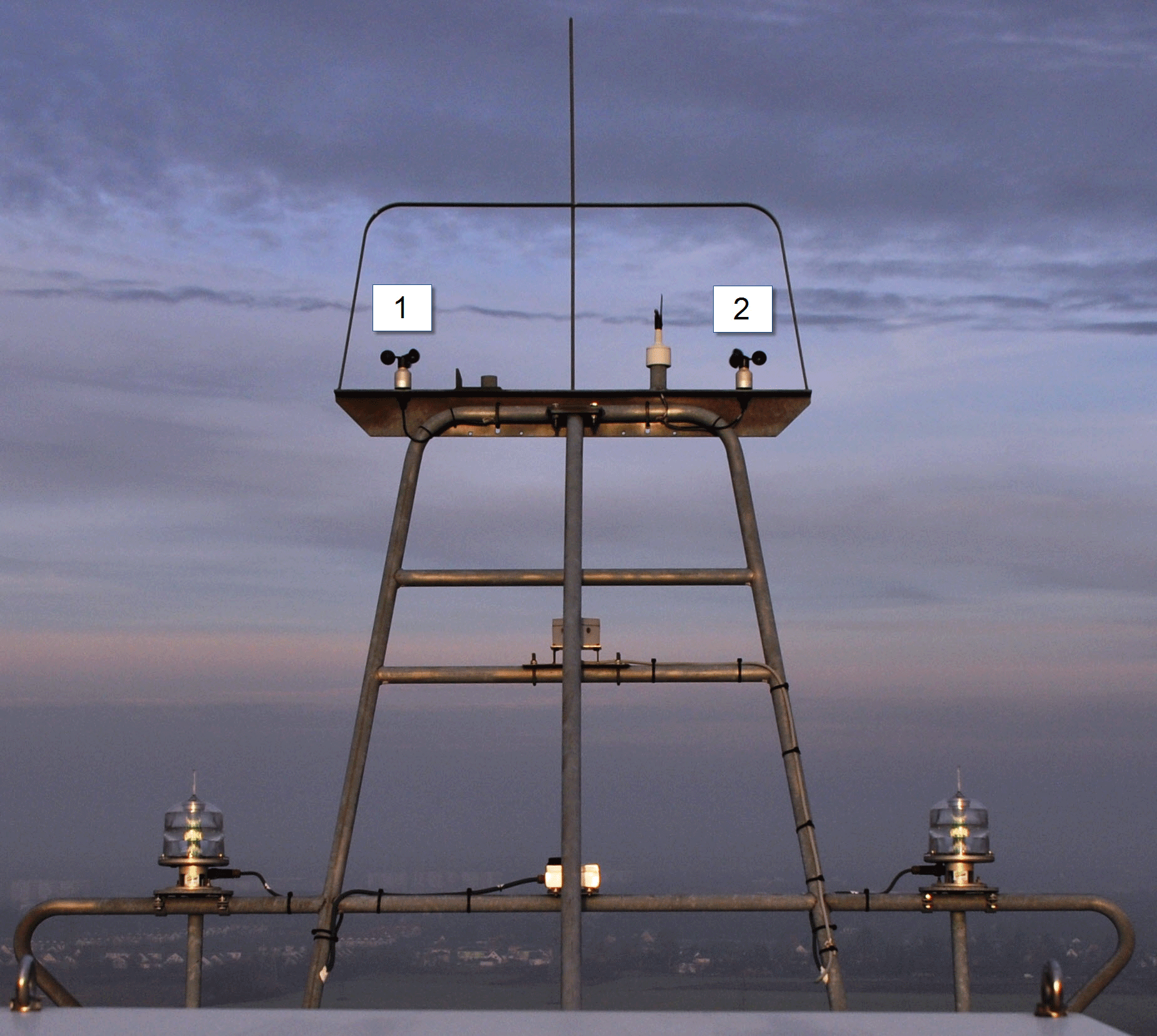
Figure 7 Typical layout of a nacelle-mounted met mast. Lightning rod, two cup anemometers (1 + 2), one wind vane and aviation lights.

Figure 7 displays a typical nacelle met mast of a turbine with two cup anemometers for redundant wind speed measurements and one wind vane for the control of the yaw system as it is used for our two reference turbines. All devices are protected with a lightning rod on top and aviation lights installed on the bottom. For this configuration the yaw error influence on the wind speed measurements is plotted in Fig. 8. The wind speed difference between the lidar in the undisturbed sector and each nacelle cup anemometer is plotted against the yaw error for different wind speed bins of the lidar.

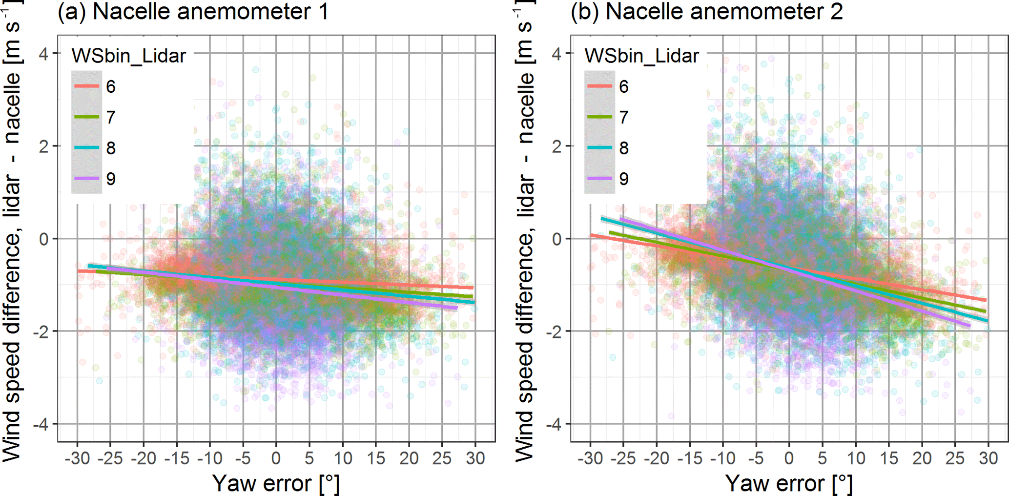
Figure 8 Wind speed difference between a ground-based lidar measuring in front of the turbine and the cup anemometers on the nacelle. The lines represent linear regressions for the respective wind speed bin (WSbin). Both 1 min wind speed measurements behind the rotor are influenced by the yaw error.

The colored lines are linear regressions with the method of least squares representing the respective wind speed bin. Both anemometers show a negative slope, which indicates a wind speed drop for positive yaw errors. A change of the yaw error γ directly changes the angle of attack at the rotor blade, with its maximum effect at vertical blade positions.

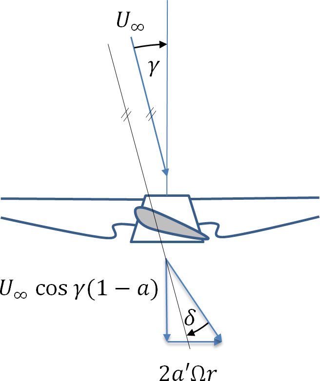
Figure 9 Illustration of the flow components behind the rotor with an axial flow a and tangential flow a^′ induction factor, where Ω is the rotor speed and r the local blade radius.

Looking at an airfoil cross section at the height of the cup anemometers (Fig. 9), a negative yaw error (wind from the left looking upwind) decreases the angle of attack and leads to a lower thrust coefficient c_T as derived from the actuator disc theory with the axial induction factor a (Burton et al., 2011):

$$\begin{array}{}\text{(4)}& c_{\mathrm{T}}=\mathrm{4}a(\cos \mathit{\gamma }-a).\end{array}$$

The flow behind the rotor can be split into an axial and a tangential part (Fig. 9). These two components are dependent on the wind speed and the rotor speed and the flow deflection function δ can be described with

$$\begin{array}{}\text{(5)}& \mathit{\delta }=\arctan \left({\displaystyle \frac{\mathrm{2}{a}^{\prime }\mathrm{\Omega }r}{U_{\mathrm{\infty }}\cos \mathit{\gamma }\left(\mathrm{1}-a\right)}}\right).\end{array}$$

In consequence the wind speed at the nacelle met mast is a function of the yaw error γ and with increasing wind speeds, when the maximum rotor speed is reached, the magnitude of this effects changes. In order to be able to apply the method of Sect. 3.1 with the nacelle wind speed device, we correct the influence of the yaw error on the wind speed by introducing the following first-order multilinear regression model with the two variables being wind speed v and yaw error γ:

$$\begin{array}{}\text{(6)}& U_{\mathrm{\infty }}={\mathit{\beta }}_{\mathrm{0}}+{\mathit{\beta }}_{\mathrm{1}}v+{\mathit{\beta }}_{\mathrm{2}}\mathit{\gamma }+\mathit{\epsilon },\end{array}$$

where the dependant variable U_∞ is the free-flow wind speed in front of the rotor, the first predictor variable v is the cup anemometer wind speed, the second predictor variable γ is the yaw error, β₁ and β₂ are estimated regression coefficients, and ε is the residual. With

$$\begin{array}{ll}{\displaystyle }{U}_{\mathrm{\infty }}& {\displaystyle }=\left[\begin{array}{c}{U}_{\mathrm{\infty }\mathrm{1}}\\ \mathrm{⋮}\\ U_{\mathrm{\infty }n}\end{array}\right],\mathit{\beta }=\left[\begin{array}{c}{\mathit{\beta }}_{\mathrm{0}}\\ {\mathit{\beta }}_{\mathrm{1}}\\ {\mathit{\beta }}_{\mathrm{2}}\end{array}\right],u=\left[\begin{array}{c}{v}_{\mathrm{1}}\\ \mathrm{⋮}\\ v_n\end{array}\right],\\ {\displaystyle }\mathit{\gamma }& {\displaystyle }=\left[\begin{array}{c}{\mathit{\gamma }}_{\mathrm{1}}\\ \mathrm{⋮}\\ {\mathit{\gamma }}_n\end{array}\right],\end{array}$$

and

$${\displaystyle }X=\left[\begin{array}{ccc}\mathbf{1}& v& \mathit{\gamma }\end{array}\right]=\left[\begin{array}{ccc}\mathrm{1}& v_{\mathrm{1}}& {\mathit{\gamma }}_{\mathrm{1}}\\ \mathrm{⋮}& \mathrm{⋮}& \mathrm{⋮}\\ \mathrm{1}& v_n& {\mathit{\gamma }}_n\end{array}\right],$$

we get

$$\begin{array}{}\text{(7)}& U_{\mathrm{\infty }}=\mathbf{X}\mathit{\beta }+\mathit{\epsilon }.\end{array}$$

The coefficients are determined from the measured data of length n with the method of least squares (ReliaSoft Corporation, 2015) described with

$$\begin{array}{}\text{(8)}& \mathit{\beta }={\left({\mathbf{X}}^{\prime }\mathbf{X}\right)}^{-\mathrm{1}}{\mathbf{X}}^{\prime }{\mathit{U}}_{\mathrm{\infty }},\end{array}$$

with the design matrix X and its transposed matrix X^′. U_∞ are the wind speed measurements in front of the rotor from the met mast or lidar, for example. The fitted model provides a new wind speed ${\widehat{U}}_{\mathrm{\infty }}$, which is much less influenced by the yaw error and can therefore be used in the methodology described in Sect. 3.1.

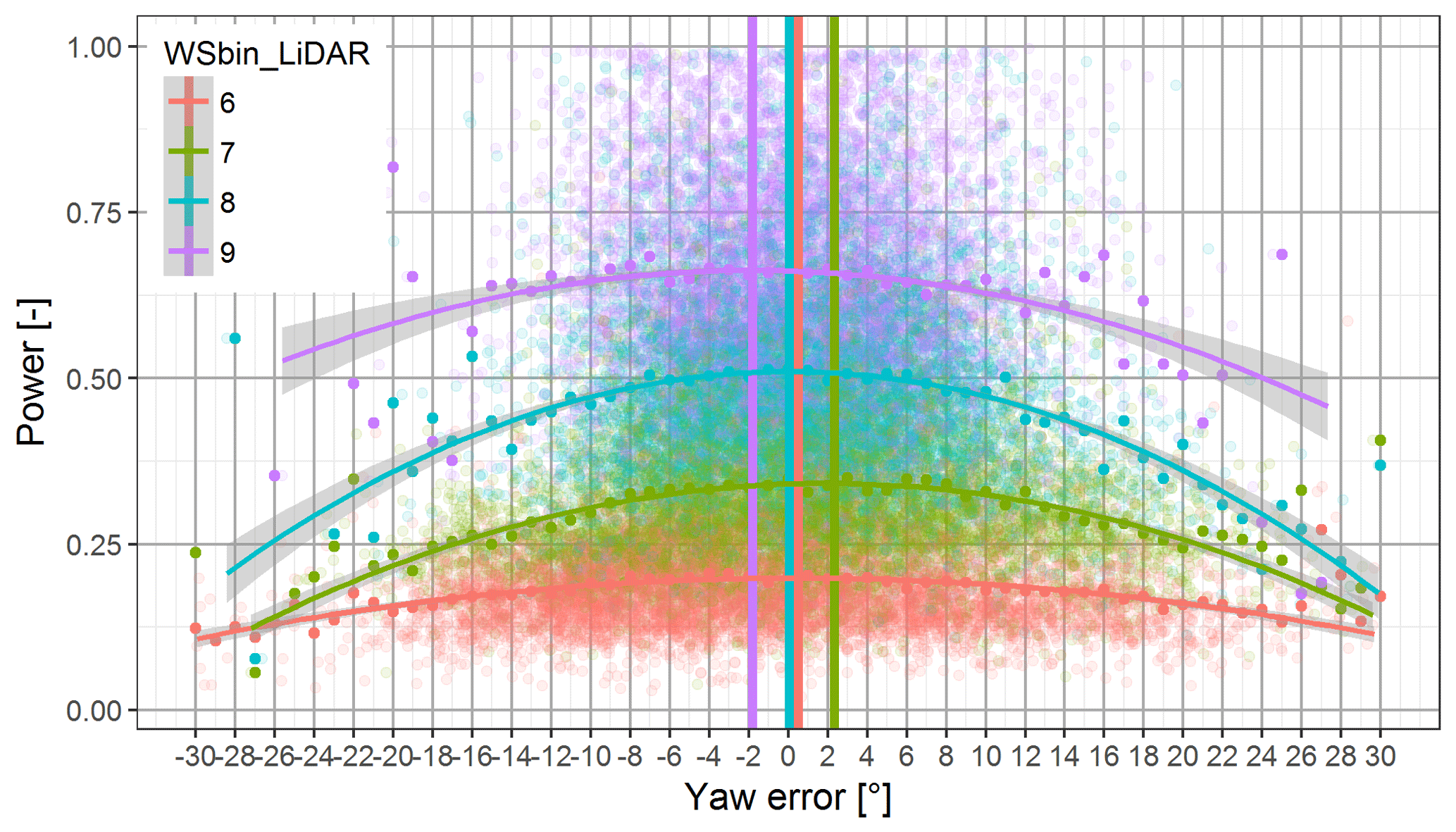
Figure 10 Determination of the optimal turbine alignment. Turbine power grouped at different wind speed bins (WSbin) measured with a ground-based lidar plotted as a function of the yaw error. The solid points represent the average value of the respective yaw error bin. The curved lines are polynomial fits based on the method of least squares. The vertical lines are the maximum of the curve, which is assumed to be the orientation of the best turbine production.

3.3 Monitoring the flow equilibrium

The aforementioned methods to determine corrections for the nacelle anemometer and wind vane are only suitable in sectors without disturbance from neighboring turbines or obstacles. But most turbines are placed in wind farms and therefore a robust method to monitor and detect orientation changes to the wind direction measurement device is needed. Mandatory precondition of the following methodology is a nacelle met mast layout similar to the one in Fig. 7. The two cup anemometers need to be placed orthogonal and symmetrical to the rotor axis and need to be of the same kind. It is not necessary to have an individual wind tunnel calibration, but the operational characteristic has to be similar. A sensitivity study on the calibration uncertainty is given in Sect. 4.4.

The wind speed difference Δ between the two cup anemometers v₁ and v₂ before the correction as described in Sect. 3.2 is dependent on the yaw error γ and its magnitude changes with the wind speed. The streamlines of a skewed flow behind the rotor (Fig. 2a) pass different radial blade positions and with the amount of the tangential flow component a^′ greater than zero the wind speed difference Δ changes for different wind speed bins. For the flow characteristic drawn in Fig. 2b, the flow streamlines behind the rotor are parallel to the rotor axis at the position of the met mast. Now the wind vane is in line with the rotor axis and measures exactly the vane assembly angle μ=φ (in our example 0^∘). We call this condition flow equilibrium since the wind speed difference Δ is approximately constant for different wind speed bins. The flow streamlines, measured at the two cup anemometers v₁ and v₂, pass approximately the same radial rotor blade position and the tangential flow component a^′ is equal to zero ($a^{\prime }=\mathrm{0}$). In contrast to Sect. 3.2 it is now necessary to use a single linear regression model without the yaw error term β₂. This additional correction would lead to more or less constant wind speed differences Δ for different wind speed bins.

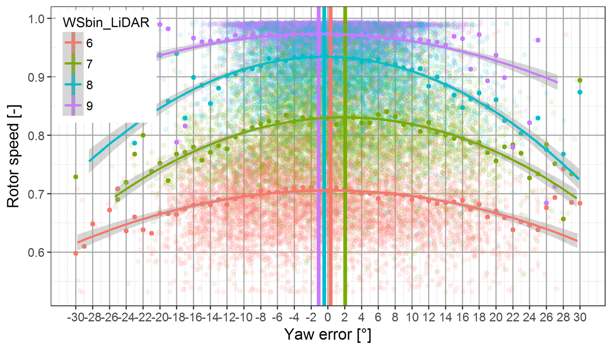
Figure 11 Determination of the optimal turbine alignment. Rotor speed grouped at different wind speed bins (WSbin) measured with a ground-based lidar plotted as a function of the yaw error. The solid points represent the average value of the respective yaw error bin. The curved lines are polynomial fits based on the method of least squares. The vertical lines are the maximum of the curve, which is the orientation of the best turbine production.

Let i and j be two different wind speed bins, then the linear regression models can be described with

$$\begin{array}{}\text{(9)}& {\mathrm{\Delta }}_i={\mathit{\beta }}_{{\mathrm{0}}_i}+{\mathit{\beta }}_{{\mathrm{1}}_i}\mathit{\mu }\end{array}$$

and

$$\begin{array}{}\text{(10)}& {\mathrm{\Delta }}_j={\mathit{\beta }}_{{\mathrm{0}}_j}+{\mathit{\beta }}_{{\mathrm{1}}_j}\mathit{\mu }.\end{array}$$

The linear regression model j is put on a level with the model i, which can be resolved to

$$\begin{array}{}\text{(11)}& \mathit{\mu }={\displaystyle \frac{{\mathit{\beta }}_{{\mathrm{0}}_j}-{\mathit{\beta }}_{{\mathrm{0}}_i}}{{\mathit{\beta }}_{{\mathrm{1}}_i}-{\mathit{\beta }}_{{\mathrm{1}}_j}}}=\mathit{\phi }.\end{array}$$

With n wind speed bins each linear regression line increases the number of intersections c as follows:

$$\begin{array}{}\text{(12)}& c={\displaystyle \frac{n\left(n-\mathrm{1}\right)}{\mathrm{2}}}.\end{array}$$

From the number of intersections ${\mathit{\mu }}_{\mathrm{1}},\mathrm{\dots },{\mathit{\mu }}_c$ the minimum, maximum and standard deviation can provide a confidence interval. Changes to the alignment of the wind direction device can be detected by repeating this calculation in regular intervals and comparing the behavior of resulting flow equilibrium over time.

4 Results and discussion

The methodology described in Sect. 3 is now tested at the two test turbines from Sect. 2.3. Both turbines are equipped with a met mast layout as shown in Fig. 7 and the data are recorded with consideration of a constant flow deflection angle δ.

4.1 Best turbine alignment

A 3-month period of 1 Hz data from Turbine WT1 is aggregated to averages of 1 min and merged with the lidar measurements. The data are filtered for a sector with free-inflow conditions and grouped into bins of 1 ms⁻¹.

Figures 10 and 11 are an example of a well-aligned turbine with a constant flow deflection angle δ. The turbine's active power and rotor speed are both normalized with its rated value and are plotted against the yaw error γ. The transparent dots represent averages of 1 min. The solid dots are yaw error bin averages (bin size 1^∘) and for each wind speed bin, differentiated with colors, a second-order polynomial fit with the method of least squares provides a convex curve. The maximum of this fitted curve is highlighted with a vertical bar and represents the orientation of the turbine with the highest production.

In Figs. 10 and 11 the vertical lines for the different wind speed bins vary between −2 and +2^∘. The wind speed bins 6 and 8 ms⁻¹ are well aligned but for the other bins a small misalignment is observed. A flow deflection function based on wind speed or rotor speed could improve this behavior. A rough assessment of the impact on the annual energy production (AEP) using a constant offset and a wind distribution with Weibull parameter A=8 and k=2 and applying the cos(γ_i)³ function as losses to the power of the respective wind speed bins results in an overall loss of ∼ 0.1 % AEP.

At lower wind speeds (6 and 7 ms⁻¹), higher turbulence causes more wind direction changes and to reduce wear of the yaw components, higher yaw errors are accepted. The range of power per bin increases with higher wind speeds because of the cubic relationship. In consequence the polynomial fit becomes more curved with higher wind speeds except for the wind speed bin 9 ms⁻¹ in which rated power is already achieved in some gusts. The solid dots, representing the yaw error bin average, follow the polynomial curve fit closely where enough data are available, but for the outer ridges the scatter increases.

The second-order polynomial fit through each wind speed bin is more curved for the rotor speed compared to the active power. This behavior helps to allocate the best alignment, except for the wind speed bin 9 ms⁻¹ in which the maximum rotor speed is already reached. Figure 12 shows the power as a function of the rotor speed and helps to understand why using the rotor speed as an independent variable provides improved fitting curves. Both variables are normalized with its maximum value. The transparent dots are averages of 1 min periods. The different colors indicate the wind speed bin (bin width of 1 ms⁻¹). The straight colored lines are linear regressions with the method of least squares. For lower wind speed bins (e.g., 6 ± 1 ms⁻¹), rotor speed has a larger variation compared to the active power and larger variation leads to a more curved fitting function. The variation in the rotor speed decreases with increasing wind speed bin but the relationship visualized with the linear regressions in Fig. 12 indicates an increased slope, which again helps to obtain a fitted curve with more bending.

Figure 12 Power as a function of rotor speed with linear regression lines per wind speed bin.

4.2 Flow correction for nacelle instruments

The same aggregated and filtered data set from the previous section is now used to fit the first-order multilinear regression model described in Sect. 3.2. The model results in

$$\begin{array}{}\text{(13)}& {\widehat{v}}_{\mathrm{1}}=\mathrm{1.17}{\mathrm{ms}}^{-\mathrm{1}}+\mathrm{0.97}{v}_{\mathrm{1}}+\mathrm{0.011}{\mathrm{ms}}^{-\mathrm{1}}{\mathrm{deg}}^{-\mathrm{1}}\mathit{\gamma },\end{array}$$

and respectively with v₂

$$\begin{array}{}\text{(14)}& {\widehat{v}}_{\mathrm{2}}=\mathrm{1.11}{\mathrm{ms}}^{-\mathrm{1}}+\mathrm{0.94}{v}_{\mathrm{2}}+\mathrm{0.03}{\mathrm{ms}}^{-\mathrm{1}}{\mathrm{deg}}^{-\mathrm{1}}\mathit{\gamma },\end{array}$$

where $\widehat{v}$ is the undisturbed wind speed from the fitted model, v₁ and v₂ are the wind speeds of the respective cup anemometers, and γ is the yaw error. The model's capability to correct the flow behind the rotor is demonstrated by a comparison of Fig. 8 with Fig. 13. Both figures show the wind speed difference between the lidar and the nacelle wind speeds plotted against the yaw error. The transparent dots are averages of 1 min periods and the horizontal lines are linear regressions with the method of least squares for the respective wind speed bins.

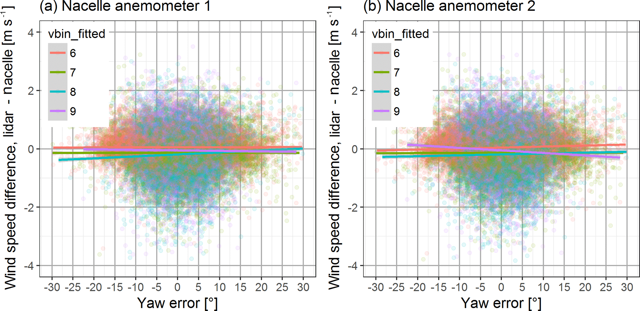
Figure 13 Wind speed difference between a ground-based measurement in front of the turbine and the cup anemometers on the nacelle after the correction with the linear model. The lines represent linear regressions for the respective wind speed bin. The dependency on yaw error is significantly reduced.

Figure 8 indicates a strong influence of the yaw error on the wind speed measurement at the nacelle instruments (with standard correction Eq. 3), leading to an underpredicted wind speed for inflow angles from the right looking upwind (positive yaw errors). In Fig. 8a the wind speed drop from a −30 to a 30^∘ yaw error is in the range of 0.4 to 1 ms⁻¹ and in Fig. 8b in a range from 1.4 to 2.6 ms⁻¹. With the new correction proposed in Sect. 3.2 this relationship becomes significantly reduced. The fitted model provides a wind speed much less dependent on the yaw error. In Fig. 13 (a and b) the wind speed drop from a −30 to 30^∘ yaw error is in the range of 0.03 to 0.5 ms⁻¹. Likewise the bias is reduced from 0.97 to 0.08 ms⁻¹ for ${\widehat{v}}_{\mathrm{1}}$ and 0.67 to 0.09 ms⁻¹ for ${\widehat{v}}_{\mathrm{2}}$. Figure 14 demonstrates the best turbine alignment method with wind speed bins of 1 ms⁻¹ from the nacelle anemometers without the correction (a) and with the correction (b) of the first-order multilinear regression model. As demonstrated in the previous section this turbine is aligned with a constant flow deflection angle δ but this fact can only be verified with the new flow correction of nacelle instruments.

The uncorrected data in Fig. 14a gives the impression that the turbine is misaligned by round about 10^∘ or more to the left. With the new flow correction of nacelle instruments applied, the estimated yaw errors are within ±3^∘, centered around 0^∘. This variation is deemed acceptable for using a constant flow deflection angle. The correction of the wind speed bias also leads to lower rotor speed values per wind speed bin.

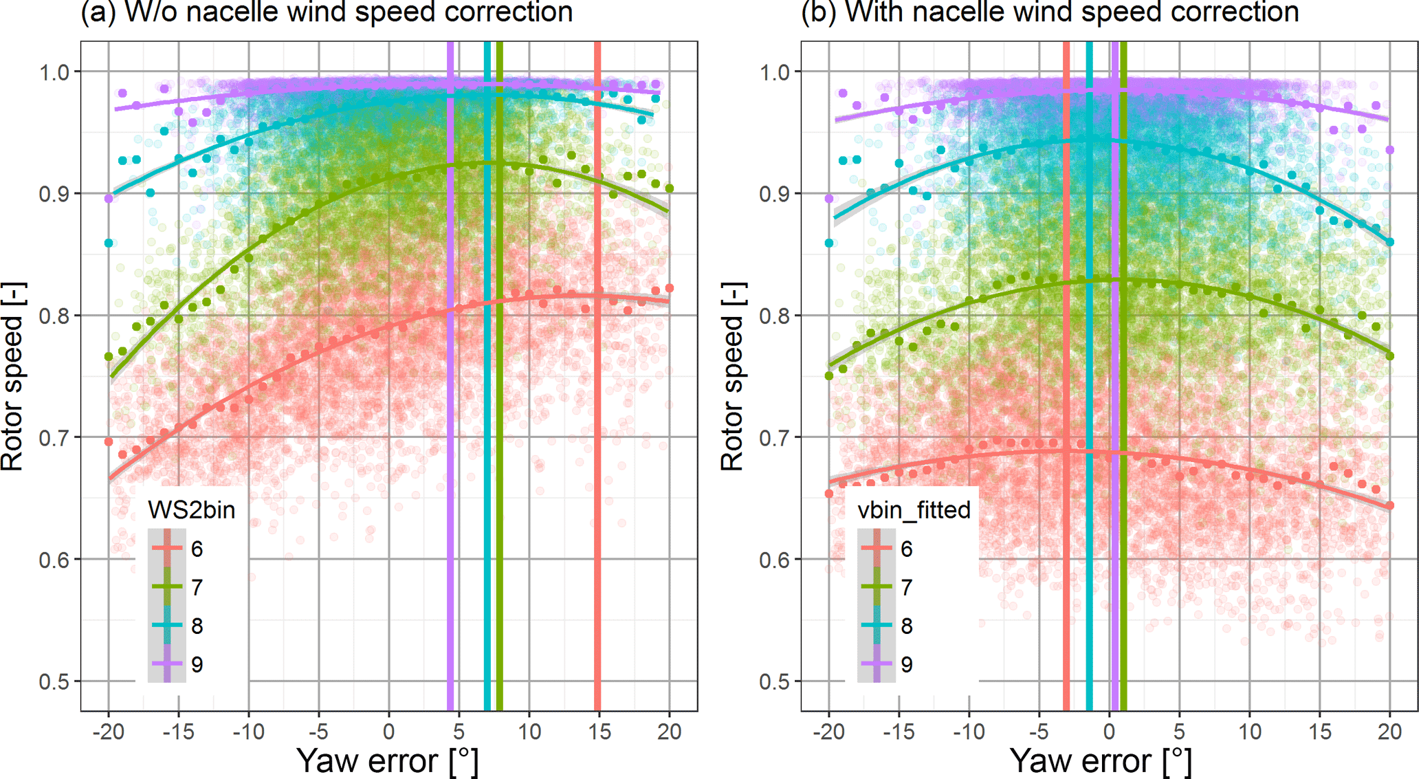
Figure 14 Best turbine alignment based on nacelle wind speed without the proposed linear flow correction of nacelle instruments (a) and with the proposed correction (b). The plot description is similar to Fig. 11. The only difference is the wind speed used for data binning.

Theoretically, the model (Eqs. 13 and 14) could now be transferred to turbines with the same flow characteristics, namely same rotor blade type and layout (e.g., sensor types and positions) of the nacelle metrology mast. A validation of this statement was not possible with the test setup due to different rotor blade modifications at the two turbines. An outlook for further improvement is a self-learning algorithm, which could be capable of using different flow deflection angles in different shear and veer conditions.

4.3 Monitoring the flow equilibrium

The flow equilibrium as described in Sect. 3.3 is calculated for two different periods of 3 days each. In Fig. 15 data with averages of 1 min are used to calculate the difference between the two nacelle anemometers as a function of the vane measurement μ for wind speed bins of 1 ms⁻¹. For each wind speed bin a linear regression model is fitted and the points of intersections between the straight lines are marked with thin black vertical lines. The median of all vertical lines is a bold red bar and is used to read the vane assembly angle φ. From the first period displayed in Fig. 15a to the second period plotted in Fig. 15b the flow deflection angle δ is changed in the control software from 0 to 7^∘. In Fig. 15a the flow equilibrium result is approximately 5.3^∘ and in Fig. 15b it returns to a value of 0.7^∘. The change of the flow equilibrium yields 6^∘. It is very likely that a software change is not fully linearly translated into the real flow conditions and the flow equilibrium provides a standard deviation which covers the correct range of the expected 7^∘ change. Therefore it is assumed that the change is detected and the results are well within sufficient accuracy.

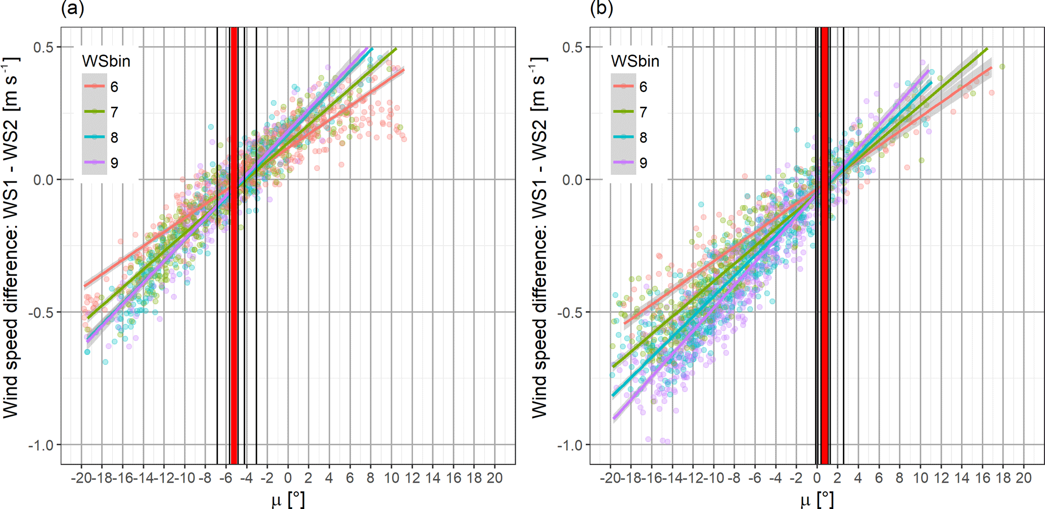
Figure 15 Flow equilibrium. Wind speed difference between the two cup anemometers as a function of the vane measurement μ. Four different wind speed bins (WSbin) provide linear regression lines and their points of intersections are marked with vertical lines. The median of the six lines is represented by the red bold vertical line and can be interpreted as vane assembly angle φ. The grey around the linear regression lines is a 95 % confidence interval.

The flow equilibrium method needs a measurement period with enough data in at least two wind speed bins to ensure that for each of these wind speed bins a linear regression model can be built and the 95 % confidence interval does not overlap the regression line of the next bin. The intersection between the models indicates the vane measurement μ=φ when the flow is parallel to the rotor axis at the location of the anemometers. In the demonstration case (Fig. 15) 3 days with averages of 1 min periods is sufficient, leading to a data count per wind speed bin of 171–625 measurements. With more than two wind speed bins we obtain further intersections. They can be used to provide a confidence interval. In our example with four wind speed bins we obtain six intersections (Eq. 12). We use the median for the final result to reduce the influence of outliers.

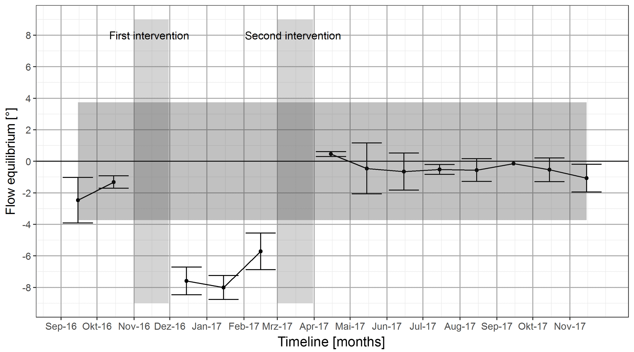
Figure 16 Monitoring the flow equilibrium with a moving window at Turbine WT2. Both changes in the alignment of the turbine are marked with vertical grey ribbons and the change in the resulting angle is clearly visible. The error bars are 1 standard deviation and the black dots are the median of all intersections per evaluation period (here: 1 month). The grey horizontal ribbon is a 90 % confidence interval.

It is now of interest to see if the proposed monitoring method is capable of detecting the two changes at Turbine WT2. Figure 16 demonstrates one possible monitoring application with the flow equilibrium method. For the total presented period only data with averages of 10 min are available. Each dot represents an evaluation performed as for one of the plots in Fig. 15 with 1 month of data. The error bars indicate 1 standard deviation added to or subtracted from the median. The horizontal transparent grey ribbon is a 90 % confidence interval (1.28 times standard deviation) of all points in the plot. The vertical transparent rectangles mark the months in which the changes are conducted. For the 2 months with interception the result is not displayed because the data set consists of two different alignments. The first 2 months were operated with a yaw error of approximately −2^∘. In November the wind vane was mechanically aligned to achieve $\mathit{\phi }=\mathrm{0}{}^{\circ }$ and the constant flow deflection angle was set to $\mathit{\delta }=\mathrm{0}{}^{\circ }$. Since the second intervention in April the turbine is operating with $\mathit{\delta }=\mathrm{7}{}^{\circ }$, which is seen as the best constant offset for the optimal aligned turbine. A flow equilibrium (black dot) within the range of ±1^∘ is seen as accurate enough as the mean standard deviation of all error bars is ±1.4^∘.

4.4 Practical guidance

In the following section we would like to give a brief summary of guidance and experience about the use of the presented method. In general, at least one of the anemometers is heated to avoid icing. In those instances, one wind speed measurement will be biased in the case of icing. An ideal setup needs two heated wind speed measurement devices. In our example, Turbine WT2 has only one heated anemometer and therefore the measured temperature is filtered to always be above 8 ^∘C.

A smaller wind speed bin size of for instance 0.5 ms⁻¹ leads to a higher number of intersections but reduces the number of measurements and this leads to higher variations in the linear regression. In our experience we obtained the best results with a bin size of 1 ms⁻¹.

The method is very sensitive to the instruments used. We only obtain good results when the same type of anemometer is used and the nacelle met mast layout is similar to Fig. 7. A mix of cup and sonic anemometer leads to wrong intersections. This opens the question about the calibration accuracy for the used anemometers. In our test case, the cup anemometers installed use the same factory provided calibration factors. Structural tolerances can lead to small differences in measurement results. For power curve verification tests, the calibration factors are usually determined in a wind tunnel for each device separately. To understand the impact of such tolerances, we have performed a sensitivity study. The evaluation in Fig. 15 is recalculated and the measurements of anemometer 1 are modified by adding an offset and in a second step by changing the slope of the linear correction function (Eq. 3).

Adding an offset on one anemometer changes only the ordinate, but the flow equilibrium delivers the same results. Different operational characteristics such as different slopes are more critical. In Fig. 17 the flow equilibrium is plotted versus the slope of the linear correction function of anemometer 1. The result from Fig. 15 is visible at the slope equal to one. With increasing slope, the flow equilibrium moves to the left. A negative yaw error would be expected.

A one percent slope difference between the anemometers leads to an error in the flow equilibrium of approximately 1.8^∘. In case of poor anemometer calibration, the assembly angle may be derived with a bias, but the monitoring application of the value is still possible. A change in operational characteristic over the life time of the anemometer has not been considered.

The method is robust against swapping anemometer 1 and 2. The slope of the linear regression line changes sign, but the result for the flow equilibrium is the same.

Figure 17 Sensitivity study. Anemometers are usually calibrated with a linear function including a slope and an offset. A change in the slope of the correction function results in a different flow equilibrium value. Both periods (a) and (b) from Fig. 15 are evaluated and the flow equilibrium is plotted as a function of the slope β₁.

With this new method, two mayor advantages are achieved, compared to the marked solutions mentioned in the introduction. Firstly, the turbine alignment is not relying on multiple wind direction measurements which reduces uncertainties caused by the challenge of finding true north. And secondly the permanent monitoring application works without the need of additional hardware which reduces the costs for operators.

5 Conclusions

This paper presented and demonstrated a three-step methodology to determine the best turbine alignment with standard nacelle-based equipment and monitor this alignment for an early detection of persistent yaw misalignment due to the vane falling out of calibration.

Step one uses a reference device (e.g., met mast or lidar) to find a correction for the wind vane to achieve the optimal power production. A constant flow deflection angle will accept yaw errors within an accuracy of ±3^∘, a correction as a function of wind speed or rotor speed could reduce the average yaw error. With a higher sampling rate of averages of 1 min periods instead of the standard 10 min average SCADA data, more extreme yaw errors can be recorded and the effect of power and rotor speed reduction is more pronounced. The use of the rotor speed instead of the power itself helps to get more curvature at the polynomial fit which is used to detect the alignment with the highest power performance. The result is independent of errors easily introduced by true north alignments of any wind direction measurement device and the optimization aims for the maximum power production which is not necessarily the case when the wind is perpendicular to the rotor plane at hub height.

Step two presents a first-order multilinear regression model to correct the flow distortion behind the rotor and enables standard turbine equipment to apply the methodology of step one without any external measurement device. Without such correction, the wind speed measurement at the nacelle is strongly influenced by the yaw error and leads to an over prediction for negative yaw errors or an under prediction for positive yaw errors.

Finally in step three the assembly angle of the wind vane is determined from SCADA data by means of a flow equilibrium using two cup anemometers of the same kind on a nacelle met mast. This is of great value as it can be used for monitoring purposes during lifetime operation with no need of additional equipment. Requirement for the metrology mast of the turbine are two heated anemometers of the same kind and one wind direction device. The operational characteristic of the two anemometers has to be the same. An offset between the two devices does not change the result, but a linear slope of more than 1 % leads to an offset in the derived flow equilibrium of approximately 1.8^∘.

In our demonstration of the monitoring methodology, two orientation changes could be detected after three days of operation with an accuracy of ±1.4^∘. We could show, that standard turbine equipment is able to align a turbine with sufficient accuracy and changes to its alignment can be detected in a reasonable short time which helps to minimize losses.