Simulation of transient gusts on the NREL 5 MW wind turbine using the URANS solver THETA

A procedure to propagate longitudinal transient gusts through a flow field by using the resolved-gust approach is implemented in the URANS solver THETA. Both the gust strike of a 1−cos() gust and an extreme operating gust following the IEC 61400-1 standard are investigated on the generic NREL 5 MW wind turbine at rated operating conditions. The impact of both gusts on pressure distributions, rotor thrust, rotor torque, and flow states on the blade are examined and quantified. The flow states on the rotor blade before the gust strike at maximum and minimum gust velocity are compared. An increased blade loading is detectable in the pressure coefficients and integrated blade loads. The friction force coefficients indicate the dynamic separation and re-attachment of the flow during the gust. Moreover, a verification of the method is performed by comparing the rotor torque during the extreme operating gust to results of FAST rotor code.

1 Introduction

The origins of applying computational fluid dynamics (CFD) to wind turbine rotors date back to the 1990s when Soerensen and Hansen (1998) applied EllipSys3D to a wind turbine. Soerensen and Hansen (1998) solved the Reynolds-averaged Navier–Stokes (RANS) equations and applied the Menter shear stress transport (SST) k−ω turbulence model to a full-scale wind turbine. In 2002 the National Renewable Energy Laboratory (NREL) performed the Unsteady Aerodynamic Experiment (UAE) (Hand et al., 2001), which has long been the reference for several CFD computations. For example, Johansen et al. (2002) presented a detached eddy simulation (DES) on the NREL UAE phase VI blade to demonstrate the capabilities of predicting flow separation. Soerensen and Schreck (2012) developed a delayed DES to investigate whether the simulation approach could be improved. Furthermore, the experiment has been widely used for URANS solver validation for example by Duque et al. (2003), Le Pape and Lecanu (2004), Yelmule and Anjuri (2013), Lynch and Smith (2013), Oe et al. (2014), and Länger-Möller (2017).

Jonkman et al. (2009) developed the generic NREL 5 MW wind turbine. Through its open-access documentation, the NREL 5 MW wind turbine is established as the reference and validation test case for single- and multi-physics test cases. For example, Chow and van Dam (2012) focused on the prediction of aerodynamic features of the wind turbine. Furthermore, they investigated the impact of fences on the flow separation in the inboard region. Full aeroelastic computations were performed by Bazilevs et al. (2011) for an isolated rotor and Hsu and Bazilevs (2012) for the rotor, tower, and nacelle. Bazilevs et al. (2011) and Hsu and Bazilevs (2012) modelled the aerodynamics with an unsteady RANS (URANS) method and the structure with shell elements. The structure properties represented the material properties of the blade. The resulting aerodynamic characteristics and blade tip deflections were good when compared to the NREL 5 MW documentation and FAST.

In the past years, growing computer power has enabled the geometry-resolved simulation of wind turbines including the sites with CFD. Studies have been performed for example by Schulz et al. (2016) or Murali and Rajagopalan (2017), who used an URANS solver to perform according studies. Moreover, hybrid large-eddy simulation (LES)–RANS approaches are implemented to analyse the behaviour of wind turbines in a complex terrain as for example presented by Castellani et al. (2017), who also considered unsteady atmospheric inflow conditions.

The challenges of correctly predicting uncertainty of the fluctuating wind loads is a research field on its own. For example, Bierbooms and Drag (1999) or Suomi et al. (2013) investigated wind fields to better understand the shape of wind gusts. Matthäus et al. (2017) argued that a detailed understanding of wind fields is not necessary. Matthäus et al. (2017) rather took into account unknowns of all parts of the wind turbine life cycle, for example changes in the blade shape due to production tolerances, ageing, or the wind field, and summarized them in uncertainty parameters to estimate the effective power outcome and rotor loads. Mücke et al. (2011) proved that turbulent wind fields do not show a Gaussian distribution as assumed in the International Electrotechnical Commission Standard (IEC). A similar conclusion was drawn by Graf et al. (2017), who investigated whether the 50-year loads as defined in the IEC adequately fulfil their purpose by applying different approaches of probability prediction to the generic NREL 5 MW turbine using the FAST rotor code.

The aerodynamic interferences between the unsteady wind conditions and wind turbines are of major importance for the prediction of fatigue loads and the annual power production. Therefore, it is part of the certification computation for each wind turbine. Nevertheless, the detailed investigation of isolated effects of the 50-year extreme operating gust (EOG) on the flow of a wind turbine using high-fidelity methods like CFD is rare even though the blade loads resulting from the extreme load cases are dimensioning load cases. In the case of vertical axis wind turbines, Scheurich and Brown (2013) analysed the power loss of a wind turbine subjected to a sinusoidal fluctuation in wind speed. However, compared to the EOG, amplitudes were small. Horizontal axis wind turbines which are hit by an EOG as defined in the IEC 61400-1 were presented by Sezer-Uzol and Uzol (2013). The wind turbine under consideration was the NREL phase VI rotor with a wind speed of 7 m s⁻¹ using the panel code AeroSIM+. The impact of the gust was then evaluated in terms of rotor thrust, torque, and wake development. Preceding this study, Bierbooms (2005) examined the flap moment of wind turbine blades, which were subjected to a gust with extreme raise, using the wind turbine design tool Bladed. Bladed is an aeroelastic software by Garrad Hassan for the industrial design and certification of wind turbines (DNVGL, 2017). Other examples of aeroelastic simulation tools for wind turbine design are HAWC2 (Larsen and Hansen, 2015) or FAST (Jonkman, 2013), which all include at least a blade element momentum (BEM) method to represent the aerodynamics, a multibody dynamics formulation to represent the structure, and an algorithm for rotational speed control. All three of them provide a possibility to compute EOG cases fully multidisciplinarily on the basis of linearized aerodynamic and structure models.

Even though the literature on gust simulations on wind turbines is not extensive, some research has been conducted in the field of aerospace science. Kelleners and Heinrich (2015) and Reimer et al. (2015) presented two approaches which are implemented in the URANS solver TAU (Schwamborn et al., 2006) to apply vertical gusts on airplanes: the velocity-disturbance approach and the resolved-gust approach. The velocity-disturbance approach adds the gust velocity to the surface of the investigated geometry. It enables the analysis of the resulting forces on the geometry surface but prevents the feedback of the structure response on the flow field and the gust shape. The resolved-gust approach overcomes the disadvantages of the one-way interaction in the velocity disturbance approach by propagating the gust through the flow field with the speed of sound. But it ignores that the gust transport velocity usually differs from the speed of sound. The validity of both implementations was demonstrated by the time history of the position of the centre of gravity, pitch angles, and load factors necessary for keeping the flight path of an aircraft constant.

In the so-called field approach, Parameswaran and Baeder (1997) added the gust velocity to the grid velocity of the computational grid to all cells with

$$\begin{array}{}\text{(1)}& {\displaystyle }x\le u\cdot t,\end{array}$$

wherein x is the coordinate in flow direction, u the gust transport velocity, and t the physical time. This approach allows the definition of a gust transport velocity and the analysis of the two-way interaction among gust, structure, and wake. Nevertheless, it requires a severe manipulation of the velocity field regardless of the flow solution that is produced by the wind turbine.

The simulation of unsteady inflow conditions of wind turbines in CFD implies several challenges. The simulation of a wind turbine including the tower is, itself, an instationary problem which needs the computation of several rotations to obtain a periodic solution. Superposed by sheared inflow profiles and instationary (stochastic) inflow conditions, periodicity can never be gained because the same flow state never occurs twice. Moreover, a computation in which the rotor motion is adapted to the actual rotor forces using a strong coupling approach as proposed by Sobotta (2015) should be included in the computation. By using strong coupling between the URANS solver FLUENT and a pitch control algorithm for the rotor motion, Sobotta has been able to implement a simulation procedure of turbine start-up. Heinz et al. (2016) performed the computation of an emergency shutdown of a turbine by using the incompressible URANS solver EllypSys3D and by neglecting the tower throughout the aerodynamic computations. Additionally, Heinz et al. considered the rotor mass and inertia by coupling the URANS solver with the aeroelastic code HAWC2.

The validation of the resolved-gust approach in the DLR URANS solver THETA (Länger-Möller, 2017; Löwe et al., 2015) is presented herein. To reduce the complexity of the problem and emphasize the quality of the resolved-gust approach, the NREL 5 MW wind turbine is chosen to operate in shear-free conditions. Moreover, the possible interferences with the structure response and speed controllers are reduced by using infinite rotor mass and inertia. Speed control algorithms are also neglected. As gust, a 1−cos()-shaped gust, which lasts about 7 s, and the EOG following the IEC standard are chosen. The resulting rotor thrust and rotor torque, pressure distributions, friction force coefficients, and the wake-vortex transport are evaluated. The rotor torque during the EOG is validated against FAST.

2 Numerical methods

2.1 Flow solver THETA

DLR's flow solver THETA is a finite-volume method which solves the incompressible Navier–Stokes (NS) equation on unstructured grids. The grids can contain a mix of tetrahedrons, prisms, pyramids, and hexagons. The transport equations are formulated on dual cells, which are constructed around each point of the primary grid. Therefore, the method is cell centred with respect to the dual grid. The transport equations are solved sequentially and implicitly. The Poisson equation, which links velocity and pressure, is solved by either the Semi-implicit Method for Pressure-Linked Equations (SIMPLE) algorithm for stationary problems or the projection method for unsteady simulations. With the projection method the momentum equations are first solved with an approximated pressure field. The pressure field is then corrected with a Poisson equation to fulfil continuity. Pressure stabilization is used to avoid spurious oscillations caused by the collocated variable arrangement.

The technique of overlapping grids (Chimera) is used to couple fixed and moving grid blocks. The method was developed by Pan and Damodaran (2002) for structured grids or Zhang et al. (2008) for unstructured grids for application in incompressible flow problems. It has been implemented in THETA by Kessler and Löwe (2014). The interpolation among the different blocks at interior boundaries is integrated in the system of linear equations on all grid levels of the multi-grid solver, leading to an implicit formulation across the blocks. This procedure was identified to be crucial for achieving fast convergence of the Poisson equation.

Implicit time-discretization schemes of first order (implicit Euler) or second order (Crank–Nicolson; backward differentiating formula, BDF) are implemented. The temporal schemes are global time stepping schemes. A variety of schemes from first order upwind up to second order linear or quadratic upwind or a central scheme and a low dissipation, low dispersion scheme (Löwe et al., 2015) are implemented. Throughout this study, the second-order central scheme is used.

The THETA code provides a user interface for setting complex initial and boundary conditions using the related C functions. This guarantees a high flexibility on the definition of boundary conditions and a straightforward modelling of very specific test cases. For example, the functions enable the prescription of gusts at the inflow boundary condition, which are then propagated through the flow field. Moreover, all physical models are separated from the basis code. Therefore, new physical models can be implemented without modification of the base code.

For turbulence modelling the commonly used Spalart–Allmaras, k–ϵ, k–ω, or Menter SST models are available. Since the early URANS computations of wind turbines the Menter SST turbulence model has been used (Soerensen and Hansen, 1998) for wind turbine applications. Recently, Länger-Möller (2017) confirmed this finding during the THETA validation by comparing the results of common one- and two-equation turbulence models to the NREL UAE phase VI experiment. Hence, the Menter SST turbulence model is applied throughout the present study. Moreover, according to the studies in Länger-Möller (2017) a time step of δt=0.006887052 s, which is equivalent to a rotor advance of $\mathrm{\Psi }=\mathrm{0.5}{}^{\circ }$ per time step, is chosen. As a time stepping scheme, the Eulerian implicit scheme for the temporal discretization is chosen. To ensure convergence in every time step, a residual of less than 10⁻⁵ has to be reached. Moreover, the solver has to perform at least 20 iterations per time step in all equations. Due to efficiency reasons, the maximum number of iterations per time step has been limited to 100.

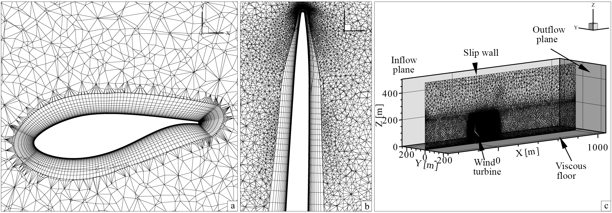
Figure 1 Computational grid set-up; (a) chord-wise distribution; (b) span-wise distribution in blade tip region; (c) cut through the flow field and boundary conditions.

2.2 FAST

The comprehensive rotor code FAST (Jonkman, 2013) is a modular software framework for computer-aided engineering (CAE) of wind turbines. FAST provides a coupling procedure to compute time-dependent multi-physics relevant for wind turbine design. By means of different modules, FAST is able to account for different physical models and turbine components in the computations. The aerodynamics are represented by a BEM method, which is based on profile polars for drag, lift, and momentum.

In the present case, most parameters remained on the default of NREL's v8.16.00a for both FAST and the NREL 5 MW wind turbine. Few parameters had to be adjusted. As it is, the variable-speed control has been turned off to ensure a constant rotational speed as in the URANS computation. The blade stiffness has been increased to the order of 10²⁹ Nm² per blade element to obtain a stiff blade. To ensure a shear-free inflow profile, the constant wind profile type without a dynamic inflow model was selected. In FAST, the EOG started after the computation of 8 s. The analytical inflow profile was included as x velocity in the IECWind file. The other wind directions were equal to 0.

3 Geometry

3.1 NREL 5 MW wind turbine

The NREL 5 MW turbine (Jonkman et al., 2009) is a three-bladed wind turbine with a rotor radius of 63.0 m and a hub height of 90 m. The rotor has a cut-in wind speed of v_ci=3 m s⁻¹ and a rated wind speed of v_rated=11.4 m s⁻¹. Cut-in and rated rotational speeds are ω_ci=41.4 ^∘ s⁻¹ and ω_rated=72.6 ^∘ s⁻¹, respectively. The blades are pre-coned and the rotor plane is tilted about β=5.0^∘ and not yawed. Along the non-linearly twisted blade seven different open-access profiles are used.

Due to the narrow gap between rotor and nacelle a valid Chimera overlap region could not be achieved in that region. Thus the nacelle of the NREL 5 MW turbine is neglected while the tower is accounted for. This approach leads to an error in the flow prediction behind the rotor hub but is supposed to have no impact on the blade loads.

The gust simulation is based on the rated wind speed v_rated=11.4 m s⁻¹. Air density of ρ=1.225 kg m⁻³ and the kinematic viscosity of $\mathit{\nu }=\mathrm{1.82}\times {\mathrm{10}}^{-\mathrm{5}}$ m² s⁻¹ is used. To isolate the gust impact of the rotor loads, a shear-free velocity profile is considered throughout the computation.

3.2 Grid characteristics

The computational grid consists of three parts. The first part contains the three rotor blades, stubs, and the rotor hub. On the blade surface, a structured grid with 156 × 189 elements in the span-wise and chord-wise directions was generated. The boundary layer mesh of the blades consists of 49 hexagon layers in an O–O topology. The height of the wall-next cell is $\mathit{\delta }=\mathrm{3}\times {\mathrm{10}}^{-\mathrm{6}}$ m along the entire blade, ensuring $y^{+}\le \mathrm{1}$. Figure 1a and b give an impression of the chord-wise and span-wise grid resolution, respectively.

The second part of the grid has the shape of a disc and contains the entire rotor. The disc measures D=166.7 m in diameter and has a depth of 26.7 m. It is filled with tetrahedrons with an edge length between 0.002 and 0.9 m. The entire disc is used as a Chimera child grid for the overlapping grid technique and contains approximately 11.63 × 10⁶ points.

The Chimera parent grid has the dimensions of $\mathrm{504}\times \mathrm{504}\times \mathrm{1512}$ m³ in width, height, and length. It contains a boundary layer grid of the floor, the tower, and a refined grid region to resolve the rotor wake up to 3R downstream.

The 54 prism layers, used to resolve the boundary layer of the viscous floor, have a total height of H=5 m with a wall-next cell height of $\mathit{\delta }=\mathrm{3}\times {\mathrm{10}}^{-\mathrm{5}}$ m. This meshing strategy enables the comparison of future gust computations that include analytically defined velocity profiles of neutral atmospheric boundary layer flows. The tower surface grid is meshed structured in a height below 5 m with 54 points in height and 180 points in the radial direction. Above 5 m, a triangulated unstructured grid is generated with the maximum edge length of 0.55 m. As the tower surface is modelled as slip wall, tetrahedrons are built directly on the tower surface.

In the Chimera parent grid, the edge length of the cells continuously grows from very small in the rotor tower and wake region to rather large close to the far-field boundaries. The entire Chimera parent grid contains approximately 13.25 × 10⁶ points.

In Fig. 1c the entire Chimera set-up is displayed and the boundary conditions are indicated. The upwind and downwind boundaries are defined as inflow and outflow, respectively. At the inflow boundary surface, the turbulence quantities and inflow velocities are prescribed. Later, the gust profile is also introduced at this boundary. The floor is defined as viscous wall. The surfaces on the top and to the left and right of the flow domain are defined as slip wall.

4 Gust modelling

4.1 The resolved-gust approach

The procedure of applying the gust to the flow field starts by computing the flow field around the wind turbine until the flow field and the global rotor loads have become periodic. For the NREL 5 MW turbine in the given set-up 9 revolutions are required. Then, the inflow velocity on the inflow boundary is modified according to the velocity change described in Sect. 4.2 or 4.3. The computation is continued so that the gust is propagated through the flow field. In the approach by Kelleners and Heinrich (2015) and Reimer et al. (2015) using TAU (Schwamborn et al., 2006) to solve the compressible RANS equations, the gust is transported with the speed of sound. In their approach, as well as in the present paper, the computation has been run at least until the gust has entirely passed the geometry in question but can be continued as long as wished by the user.

The restrictions to ensure a loss-free transport of the gust velocity on the resolved-gust approach named by Kelleners and Heinrich (2015) or Reimer et al. (2015) are

• a fine grid upstream of the geometry in question

• a fine time step.

As THETA is an incompressible solver, the speed of sound is infinite. In addition to the strong implicit formulation and the choice of boundary conditions that prevent the flow from escaping sideways, this leads to a spread of the gust velocity through the flow field instantaneously. If the same gust velocity is added to the constant inflow condition in every point in the inflow plane and the boundary conditions are chosen as specified in Sect. 3.2, the transport of the gust velocity will be loss free and instantaneous through the entire domain and on the far-field boundaries. Hence, the restrictions by Kelleners and Heinrich (2015) and Reimer et al. (2015) concerning the grid resolutions are obsolete, while a fine time step is required to ensure numerical stability.

To analyse the resolved-gust approach in the incompressible URANS solver THETA, the inflow velocity profile is shear free and the gust velocity remains independent of the height above ground.

Figure 2 Inflow velocity with dependence on physical time t.

4.2 Cosines gust

The 1−cos() gust is modelled analogously to the EASA certification standard (EASA, 2010) as

$$\begin{array}{}\text{(2)}& {\displaystyle }u\left(t\right)=u_{\mathrm{g}}\left(\mathrm{1}-\cos \left({\displaystyle \frac{\mathrm{8}\mathit{\pi }}{H}}\right)\right),\end{array}$$

with u(t) and u_g as the time-dependent velocity and the gust velocity, respectively, and H as the gust gradient. In the work presented, H is chosen to generate a non-compressed sinusoidal gust

$$\begin{array}{}\text{(3)}& {\displaystyle }H={\displaystyle \frac{\mathrm{8}\mathit{\pi }}{t-T_{\mathrm{S}}}},\end{array}$$

wherein t represents the actual physical time and T_S is the time at which the gust starts. Inserting Eq. (3) in Eq. (2) the following definition of the gust results:

$$\begin{array}{}\text{(4)}& {\displaystyle }u\left(t\right)=\left\{\begin{array}{ll}{u}_{\mathrm{g}}\left(\mathrm{1}-\cos (t-T_{\mathrm{S}})\right)& \mathrm{\text{if}}{T}_{\mathrm{S}}\le t<T_{\mathrm{S}}+T_{\mathrm{g}}\\ u& \mathrm{\text{if}}t\le T_{\mathrm{S}}\text{or}t\ge T_{\mathrm{S}}+T_{\mathrm{g}}\end{array}\right.,\end{array}$$

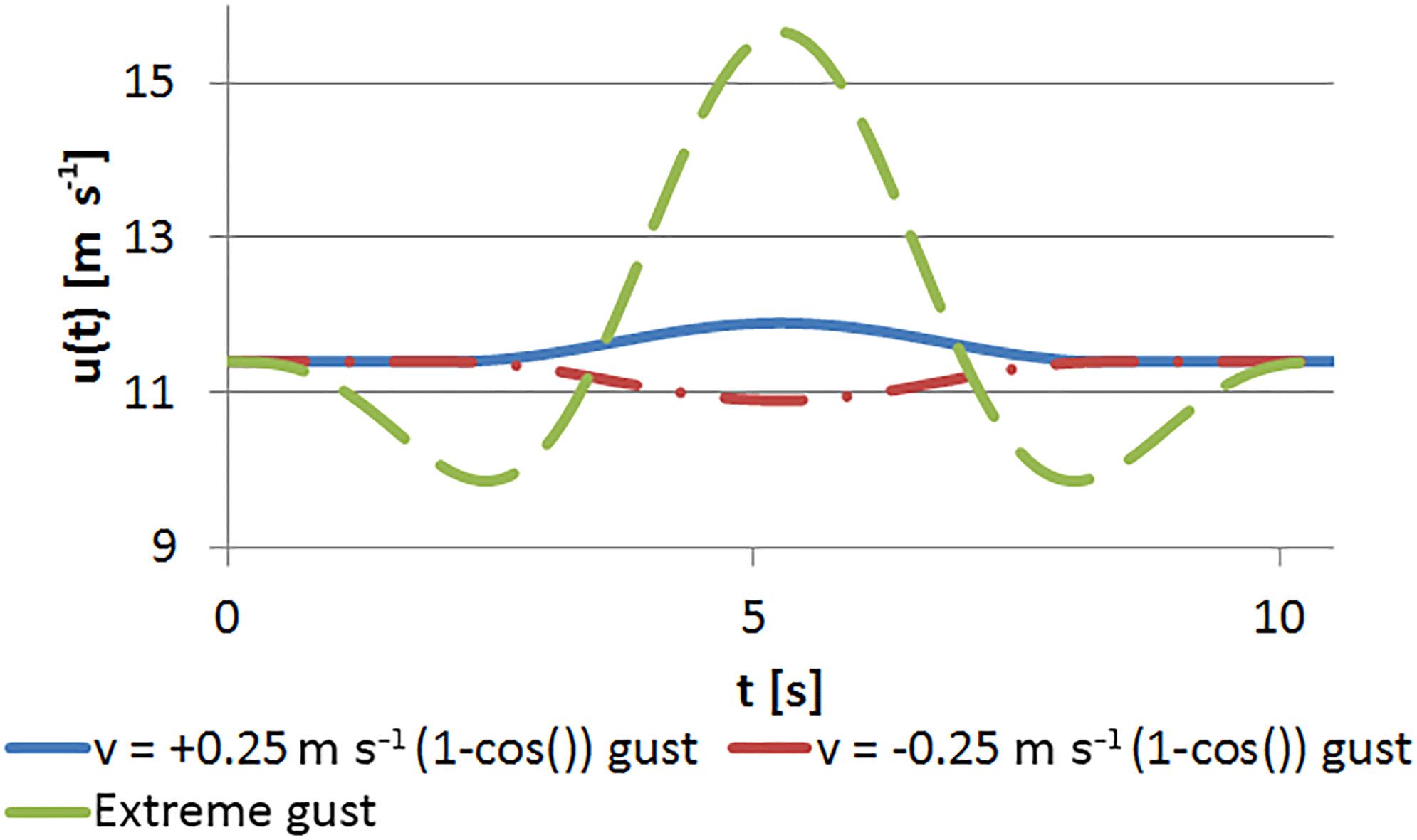
wherein T_g is the duration time of the gust. The gust velocity u_g is defined as +0.25 m s⁻¹ representing a gust and −0.25 m s⁻¹ representing a sudden calm. In both cases, the maximum change in wind speed is 0.5 m s⁻¹ or 4.4 % at rated wind speed of the NREL 5 MW turbine. The turbulence intensity of the 1−cos() gust is 2.5 %, which is on the order of the atmospheric turbulence intensity that Schaffarczyk et al. (2017) found in a field measurement campaign on a horizontal axis wind turbine. The resulting gust profile of the present study is displayed in Fig. 2.

4.3 Extreme operating gust

The time-dependent velocity change of the EOG is modelled following the IEC 61400-1 standard.

$$\begin{array}{}\text{(5)}& {\displaystyle }u(z,t)=u\left(z\right)-\mathrm{0.37}\cdot u_{\mathrm{g}}\sin \left({\displaystyle \frac{\mathrm{3}\mathit{\pi }\cdot t}{T_{\mathrm{g}}}}\right)\cdot \left(\mathrm{1}-\cos \left({\displaystyle \frac{\mathrm{2}\mathit{\pi }\cdot t}{T_{\mathrm{g}}}}\right)\right),\end{array}$$

wherein T_g=10.5 s is the characteristic time as defined in the IEC 61400-1 (2005), t the physical time simulated, u(z) the velocity profile depending on the height, and u_g the gust velocity. The latter is defined as

$$\begin{array}{}\text{(6)}& {\displaystyle }{u}_{\mathrm{g}}=\mathrm{3.3}\left({\displaystyle \frac{{\mathit{\sigma }}_{\mathrm{1}}}{\mathrm{1}+\mathrm{0.1}\left(\frac{D}{{\mathit{\lambda }}_{\mathrm{1}}}\right)}}\right)\end{array}$$

and is 5.74 m s⁻¹ in the given case. In Eq. (6), ${\mathit{\sigma }}_{\mathrm{1}}=\mathrm{0.11}\cdot u_{\mathrm{hub}}$ is the standard turbulence deviation, λ₁=42 m the turbulence scale parameter, and D the rotor diameter. u_hub represents the velocity at hub height. The velocity u_e1 is the average over 10 min with a recurrence period of 1 year. It is defined as

$$\begin{array}{}\text{(7)}& {\displaystyle }{u}_{\mathrm{e}\mathrm{1}}=\mathrm{1.12}\cdot u_{\mathrm{ref}}{\left({\displaystyle \frac{z}{z_{\mathrm{hub}}}}\right)}^{\mathrm{0.11}},\end{array}$$

with the reference velocity v_ref=50 m s⁻¹. It is defined in the IEC 61400-1 standard for a wind turbine of the wind class A1. In a shear-free flow, the inflow velocity is constant with height and thus u(z) reduces to u and u(z,t) to u(t). By additionally entering Eq. (7) in Eq. (5) one obtains the final gust definition

$$\begin{array}{}\text{(8)}& {\displaystyle }u\left(t\right)=u-\mathrm{0.37}\cdot u_{\mathrm{g}}\sin \left({\displaystyle \frac{\mathrm{3}\mathit{\pi }\cdot t}{T_{\mathrm{g}}}}\right)\cdot \left(\mathrm{1}-\cos \left({\displaystyle \frac{\mathrm{2}\mathit{\pi }\cdot t}{T_{\mathrm{g}}}}\right)\right).\end{array}$$

The resulting gust profiles of the EOG in comparison to the moderate 1−cos() gust is visualized in Fig. 2.

5 Results

5.1 Constant inflow conditions

As described in Sect. 4.1 a periodic flow field with periodic rotor loads is mandatory as starting conditions for computing gusts that act on wind turbines. The resulting time history of rotor thrust F_x and rotor torque M_x for constant inflow conditions over revolutions 6 to 10 are displayed in Figs. 3 and 4 with the red line. In both figures the periodic behaviour of a periodic flow field is visible as well as the typical 3 ∕ rev characteristic of a rotor tower configuration of the wind turbine. By averaging rotor thrust F_x and torque M_x about 4 revolutions, one obtains 738.9 kN and 4.15 × 10⁶ Nm, respectively. Compared to the reference of Jonkman et al. (2009), at rated conditions the values deviate by about approximately −3.77 and −0.98 %, respectively. Imiela et al. (2015) achieved a rotor thrust of 786 kN and a torque of 4.4 × 10⁶ Nm in their studies with the compressible URANS solver TAU for the stiff-bladed NREL 5 MW turbine.

The agreement among the URANS computations performed with THETA, TAU, and the reference documentation of the NREL 5 MW wind turbine (Jonkman et al., 2009) is excellent. Thus, the numerical set-up is validated successfully.

Figure 3 Rotor thrust F_x during the gust.

Figure 4 Rotor torque M_x during the gust.

Between $\mathrm{\Psi }=\mathrm{3060}{}^{\circ }$ and $\mathrm{\Psi }=\mathrm{3240}{}^{\circ }$, in the eighth revolution, high-frequency oscillations occur in the THETA computation. In the specific time step, the Poisson equation for pressure correction has not converged in the maximum number of iterations. Nevertheless, the interference subsides in the following rotor rotations and is sufficiently small. Thus, the reason for this oscillation is of minor importance in the context of this paper.

If the wind turbine operates in uniform flow conditions, a 3 ∕ rev characteristic is found in both F_x and M_x, which is caused by the tower blockage effect. Moreover, the constant amplitudes around a steady mean value of both F_x and M_x indicate that the flow field has converged. The converged state includes the boundary layer that developed on the viscous floor of the flow domain. Over the length of the entire flow domain, the boundary layer achieved a thickness of approximately 1 m at the end of the flow domain. This is far below the rotor area and does not affect the rotor characteristics or wake development during the computation. Hence, the gust as defined in Eqs. (4) or (8) can be applied in the next step.

5.2 Cosine gust

The impact of the 1−cos() gust on rotor thrust F_x and rotor torque M_x during the gust is evaluated by comparison to uniform inflow conditions. F_x and M_x are displayed in Figs. 3 and 4, respectively. Therein, the period between 30 and 50 s is displayed while the gust operates between T_S=37 s and $T_{\mathrm{S}}+T_{\mathrm{g}}=\mathrm{44}$ s. Thus, it lasts approximately 1.5 rotor revolutions. As expected, the gust velocity spreads over the entire field immediately and also affects rotor thrust and rotor torque instantaneously. In the case of gust and calm no hysteresis effect is found as rotor thrust and rotor torque recover immediately after the gust. This is visible in both Figs. 3 and 4 as the curve of constant inflow conditions is matched right after 44 s. The symmetric response of rotor thrust and rotor torque to the gust is caused by the modelling assumptions of a stiff blade and a missing speed control algorithm.

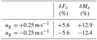
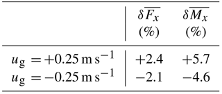
Table 1 Gust-induced peak loads on the rotor during the 1−cos() gust in relation to the constant blade load.

During the gust, F_x and M_x follow the modification of the inflow condition. Hence, for a positive gust velocity u_g (Eq. 4) rotor loads increase in a 1−cos() shape while they decrease in the same manner for a negative gust velocity. Additionally, the tower blockage effect is superposed on the blade loads and remains detectable in the blade load development. In the case of $u_{\mathrm{g}}=+\mathrm{0.25}\mathrm{m}/\mathrm{s}$, the tower blockage effect reduces the time that the rotor experiences maximum loads, as is visible at approximately t=41 s. A sharp drop in both rotor thrust and rotor torque is visible. This drop is due to the tower blockage effect and would have appeared at a different instance of the gust if the rotor position at the gust starting time was different. Nevertheless, during the calm with $u_{\mathrm{g}}=-\mathrm{0.25}\mathrm{m}/\mathrm{s}$ the tower blockage leads to an additional decrease in rotor thrust and rotor torque at t=41 s. The rapid changes in rotor thrust and rotor torque indicate the fast load changes on the blade which increase fatigue loads.

Table 1 lists the relative differences in F_x and M_x during the gust, computed by Eq. (9). In Eq. (9) the subscript “max” indicates the extreme rotor loads and the overline the averaged rotor loads under constant inflow conditions of Sect. 5.1.

$$\begin{array}{ll}{\displaystyle }& {\displaystyle }\mathit{\delta }{F}_x=\mathrm{100}\cdot \left({\displaystyle \frac{F_{max}}{\stackrel{\mathrm{‾}}{F_x}}}-\mathrm{1}\right)\\ \text{(9)}& {\displaystyle }& {\displaystyle }\mathit{\delta }{M}_x=\mathrm{100}\cdot \left({\displaystyle \frac{M_{max}}{\stackrel{\mathrm{‾}}{M_x}}}-\mathrm{1}\right)\end{array}$$

Additionally, the relative difference in the averaged blade load is computed by first integrating rotor thrust and rotor torque during the gust excitation and then computing Eq. (9). The result of the gust peak load is listed in Table 1 while the integrated loads are contained by Table 2.

In both tables it can be seen that a reduction of the wind speed due to calm or the increase in the wind speed with the same amplitude leads to very similar absolute changes in rotor thrust and rotor torque. By comparing the values of Tables 1 and 2 it is also found that the absolute peak loads are 2.3 times larger than the averaged loads. Thus, the use of maximum loads during a 10 min interval is inevitable for a computation of equivalent fatigue loads while averaging the loads is not appropriate.

It is also important to note that the rotor loads return to the values of constant inflow conditions right after the gust ended. This indicates that there are neither reflections nor numerical oscillations, which lower the numerical accuracy, in the flow field. In summary, the behaviour of rotor thrust F_x and rotor torque M_x is as expected. The increased wind speed causes higher thrust and momentum and vice versa while the amplitude is identical for the increase and decrease in wind speed.

Table 2 Averaged rotor loads during the 1−cos() gust in relation to the constant blade load.

By considering blade deflections and changes to the rotational speed in future aeroelastic computations, the resulting rotor torque and rotor thrust will change.

Figure 5 Rotor thrust F_x and torque M_x during the gust.

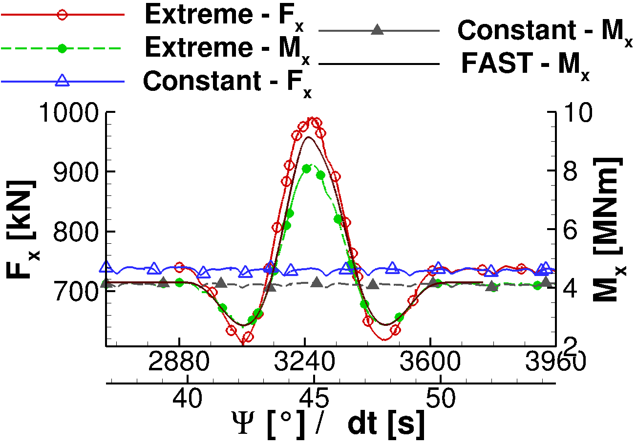
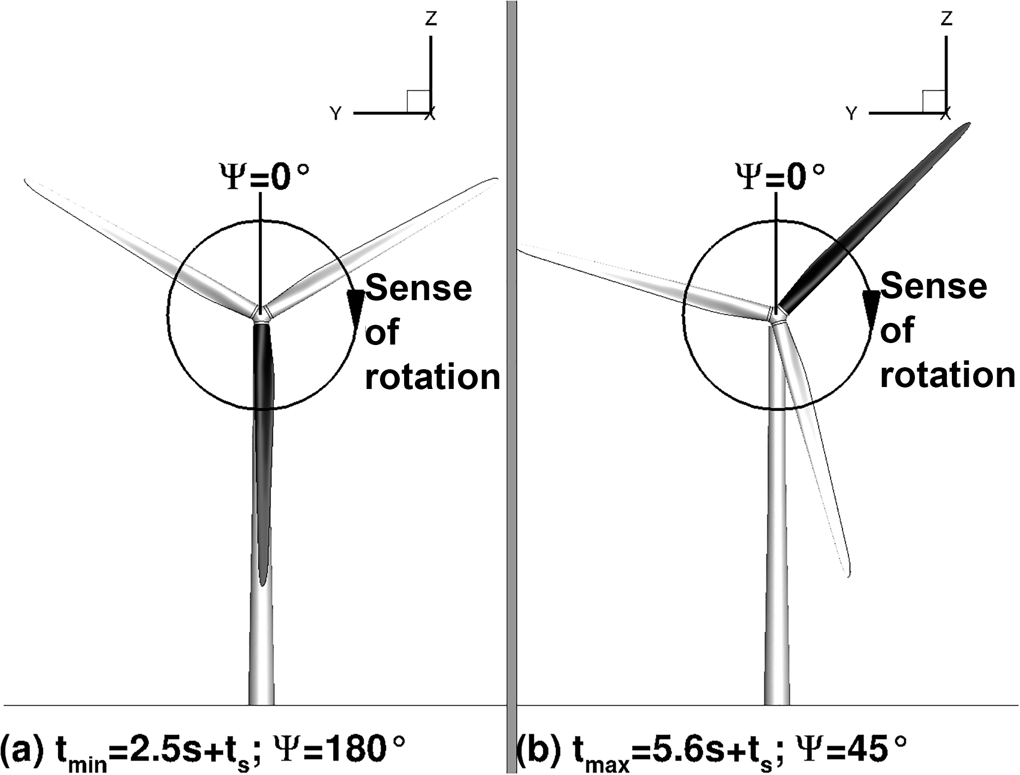
Figure 6 Rotor position at minimum (a) and maximum (b) gust velocity; black blade is blade number 1.

5.3 Extreme operating gust

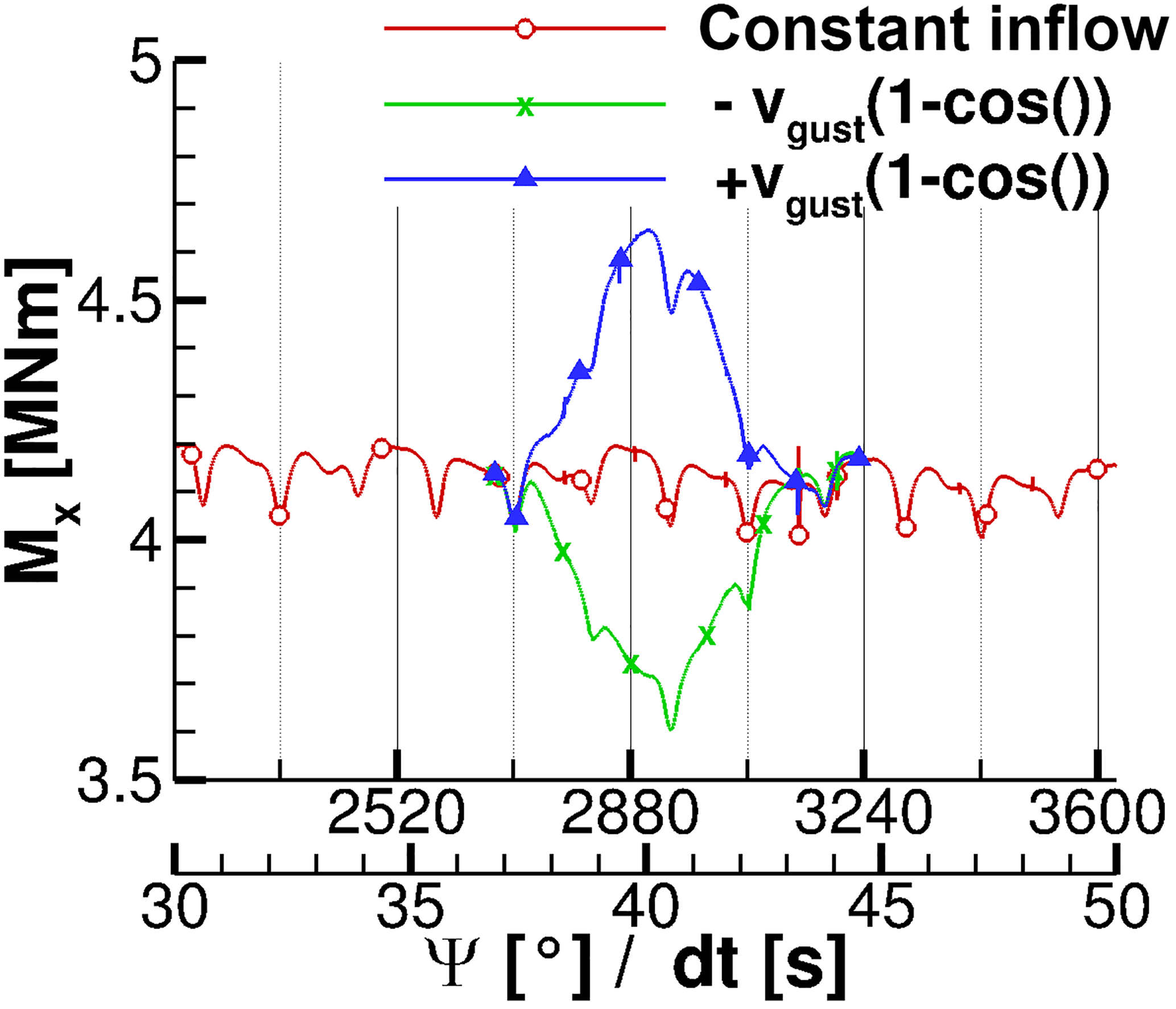
Figure 5 presents rotor thrust F_x and rotor torque M_x during the EOG excitation in comparison to the constant inflow conditions. Moreover, the rotor torque that is computed by FAST for a stiff blade and constant rotational speed is displayed. The EOG lasts about 0.5 s or 2 rotor revolutions. In comparison to the rotor loading during the 1−cos() gust (Sect. 5.2) the tower blockage effect becomes negligible. Hence, the starting position of the rotor is less important for the computation of maximum loads. This is also seen in the FAST result. By comparing the rotor torque during the gust of THETA to the one of FAST it is found that both values coincide exactly before t=43.5 s and after t=46.5 s. Between these two time stamps, FAST predicts significantly higher loads than THETA. Moreover, the EOG load at the maximum gust velocity is increased in comparison to THETA. The differences result from the flow characteristics of the blade. THETA predicts large areas of flow separation as a response to accelerated velocity after t=43.5 s. The flow reattaches over most of the blade after t=46.5 s when the velocity slowed down sufficiently. It is most likely that the profile polars that the BEM of FAST relies on is not able to reproduce the instationary flow behaviour of the given case.

Figure 7 Span-wise distribution of (a) rotor thrust and (b) rotor torque for different azimuth positions at constant inflow and during the gust.

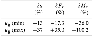
The maximum velocity u_max during the gust is about 15.65 m s⁻¹ and the minimum velocity u_min is 9.94 m s⁻¹, which is 137 and 87 % of the values at rated wind speed. The changes in rotor thrust and rotor torque, computed using Eq. (9), are given in Table 3. It is shown that the rotor torque is decreased by 36 % during the calm that precedes or follows the velocity maximum and increased about 100 % during the gust peak. The changes in rotor thrust are smaller even though the amplitudes of load change are significant as well.

Figure 8 Pressure distribution of the blade at the inboard section, (a, c) undisturbed flow, and (b, d) with tower blockage; (a, b) pressure distribution and (c, d) friction force coefficient.

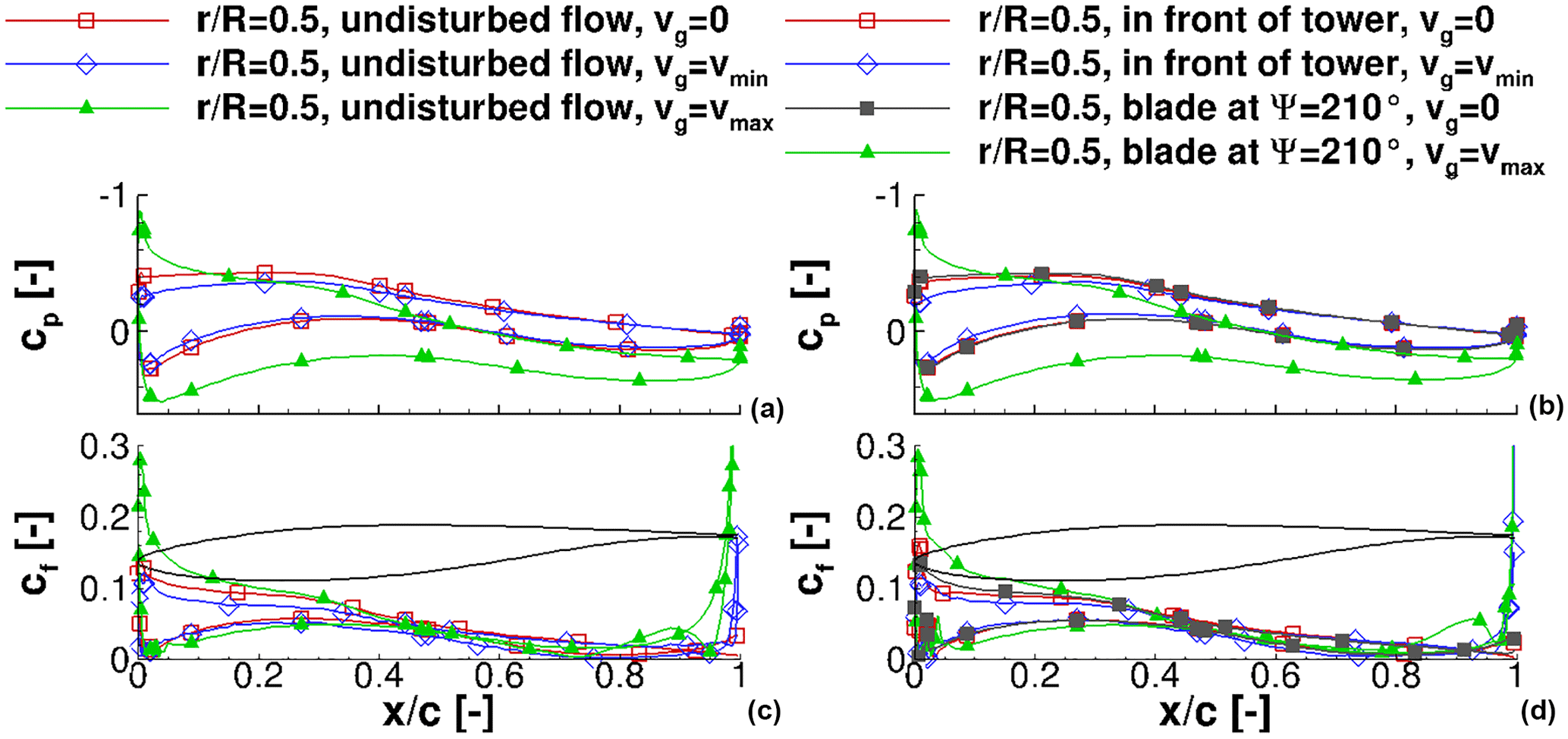
Figure 9 Pressure distribution of the blade at the midsection, (a, c) undisturbed flow, and (b, d) with tower blockage; (a, b) pressure distribution and (c, d) friction force coefficient.

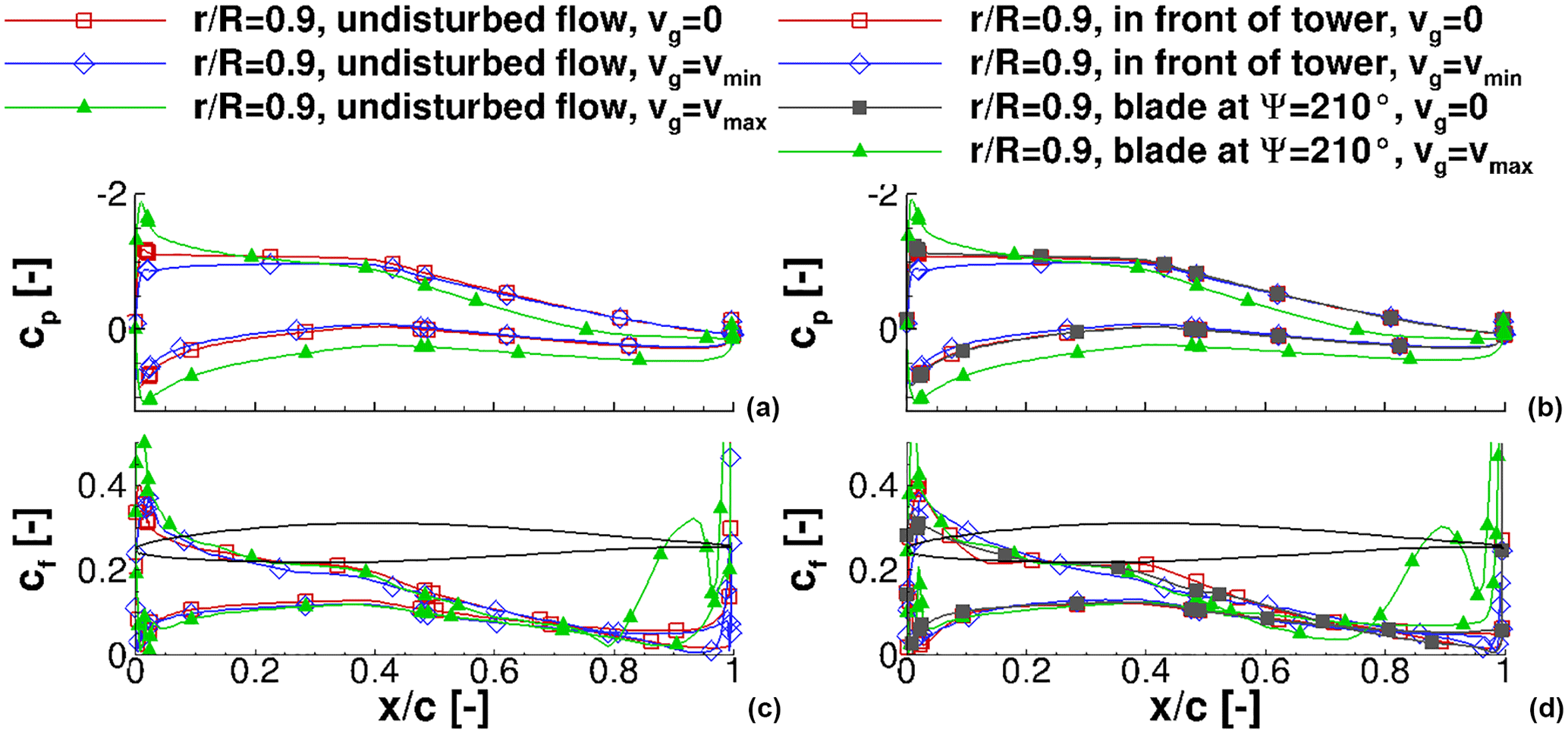
Figure 10 Pressure distribution of the blade at the outboard section, (a, c) undisturbed flow, and (b, d) with tower blockage; (a, b) pressure distribution and (c, d) friction force coefficient.

To analyse the flow state on the blade during the gust, two instances have been chosen: after $t_{min}=\mathrm{2.5}\mathrm{s}+T_{\mathrm{S}}=\mathrm{42}$ s (minimum gust velocity) and $t_{max}=\mathrm{5.6}\mathrm{s}+T_{\mathrm{S}}=\mathrm{45}$ s (maximum gust velocity). Figure 6a and b, respectively, display the rotor positions in the instances investigated. In both figures blade number 1 is coloured in black. At t_min, when the gust is at its minimum velocity, blade number 1 is right in front of the tower and additionally experiences the tower blockage effect. Conversely, at t_max, when the gust is at its maximum velocity, blade number 1 is in free-stream conditions while the flow on blade number 3 enters the tower blockage region. The impact of the tower blockage during the constant inflow conditions at t_min and t_max is visible in the radial distribution of rotor thrust and rotor torque (Fig. 7).

Table 3 Gust-induced peak load during the EOG on the rotor in relation to the constant blade load.

In accordance to Fig. 5 the overall rotor loading is reduced when the blade experiences minimum gust velocity. Conversely, a significant increase in rotor loading is observed when the blade experiences the maximum gust velocity. At all times, the rotor thrust is reduced only slightly by the tower blockage effect. Moreover, only the inboard part of the rotor appears to be affected by the tower blockage. Contrariwise, the rotor torque is affected by the tower blockage in the outer part of the rotor. In addition, the tower blockage effect generally has only a small impact on the rotor torque at wind velocities smaller than rated wind speed. With the maximum gust velocity, the blade at $\mathrm{\Psi }=\mathrm{210}{}^{\circ }$ experiences a strong tower blockage effect that reduces the rotor torque up to 29 % (radial section $r/R=\mathrm{65}$ %). The reason is the different separation behaviour at the trailing edge of the blade, which is investigated through pressure coefficient distributions and friction force coefficients at three radial sections: an inboard section at $r/R=\mathrm{10}$ %, a midsection at $r/R=\mathrm{50}$ %, and an outboard section at $r/R=\mathrm{90}$ %. They are displayed in Figs. 8, 9, and 10, respectively.

In all three figures the pressure is displayed in the upper half and is normalized with the vector sum of the tip speed and the constant inflow velocity. For a meaningful comparison to constant inflow conditions, it was ensured that the investigated sections result from blades at the same azimuth positions.

A noticeable difference in c_p at minimum gust velocity is found in all sections (Figs. 8a, 9a, and 10a) when compared to the constant inflow conditions. The decrease in the stagnation point of c_p to lower values at t_min is higher than that of the tower blockage effect while otherwise the pressure distributions keep the general shape. Conversely the difference between constant inflow conditions and the maximum gust is significantly higher. The maximum c_p increased about 58 % at the blade tip. Moreover, the shape of the pressure distribution changes over the entire blade. This is visible especially in the mid-board and outboard blade sections (Figs. 9a and 10a). In both sections, the pressure increases rapidly in the rear half of the upper blade surface and even reaches positive values in the last 20 % of the profile. This behaviour is a first indication of a separation region and reversed flow around the trailing edge.

The friction coefficients on the blade sections in undisturbed flow are displayed in Figs. 8c, 9c, and 10c. In all sections, strong fluctuations, which result from the truncated geometry at $x/c=\mathrm{1}$, are visible at the trailing edge. The friction force coefficient c_f in the inboard section (Fig. 8c) shows large differences among all considered time instances. The oscillations around $x/c=\mathrm{50}$ % at constant inflow conditions indicate a small separation region with otherwise attached flow. At minimum gust velocity the overall friction force level is increased around the leading edge and the separation region has shifted upward and is between $x/c=\mathrm{20}$ % and $x/c=\mathrm{40}$ %. At the maximum gust velocity, the friction force is increased and the oscillations between $x/c=\mathrm{20}$ % and $x/c=\mathrm{50}$ % indicate a larger separation region on the upper blade surface. The friction force coefficient indicates that separation in the blade inboard section is present during the entire rotor rotation. It is triggered through the close cylindrical blade root and amplified with higher inflow velocities.

Conversely to the inboard section, changes in separation at the midsection appear due to the gust only. In Fig. 9c the friction force level is decreased at minimum gust velocity and the curve is very smooth. At maximum gust velocity, small oscillations appear around $x/c=\mathrm{90}$ %, indicating separation in that region. By increasing the rotor radius, the behaviour is enforced. At the outboard section (Fig. 10c), the local maximum in c_f in the last 20 % of the profile almost reaches the level of the leading edge at t_max.

The same analysis is performed for the blade that is situated right in front of the tower or at $\mathrm{\Psi }=\mathrm{210}{}^{\circ }$. For the pressure distributions (Figs. 8b, 9b, 10b) the same effects as described for the blades in undisturbed flow are found. The only difference is that due to the tower blockage the overall pressure level is decreased by about 1 %. This enforces the observation from the rotor thrust and rotor torque time histories in Figs. 5 and 7. Namely, the tower blockage effect is small compared to the EOG operating loads. Conversely, the characteristics of friction forces (Figs. 8d, 9d, and 10d) in the inboard and outboard sections differ from those of the blades in undisturbed flow. In the inboard section in Fig. 8d, the oscillations in c_f reduce to a minimum while the overall friction force level remains constant. Only at maximum gust velocity, do the oscillations around the trailing edge appear. Thus, the tower seems to suppress separation and it takes some time until the separation state is fully recovered. The friction force coefficient in the midsection behaves similarly to the inboard section with the difference that the entire separation region is larger (Fig. 9d). In the outboard section in Fig. 10d, the friction force is increased significantly due to the maximum gust velocity. By comparing the friction coefficients of the blades in undisturbed flow and in the tower blockage region, it is found that the separation on the suction side of the blade covers a larger area in the rear part of the blade. The separation induces a larger profile thickness, which results in a different induced angle of attack and thus reduced momentum.

Finally, the transport of the tip vortices is investigated. It has to be understood as an indication of whether the velocity transport in the field works as expected but the tip vortex transport has only small meaning for the transient rotor loading during the gust. In addition, the velocity in the field changes gradually because of the infinite speed of sound in the entire flow domain. Thus, the vortices that are shed from the blade at a given wind speed are not transported with their specific gust transport velocity. Contrariwise, all existing vortices experience identical changes in the gust transport velocity. Thus, the geometrical distance between existing vortices remains constant.

Figure 11 Tip vortex transportation in the vertical plane through the rotor centre.

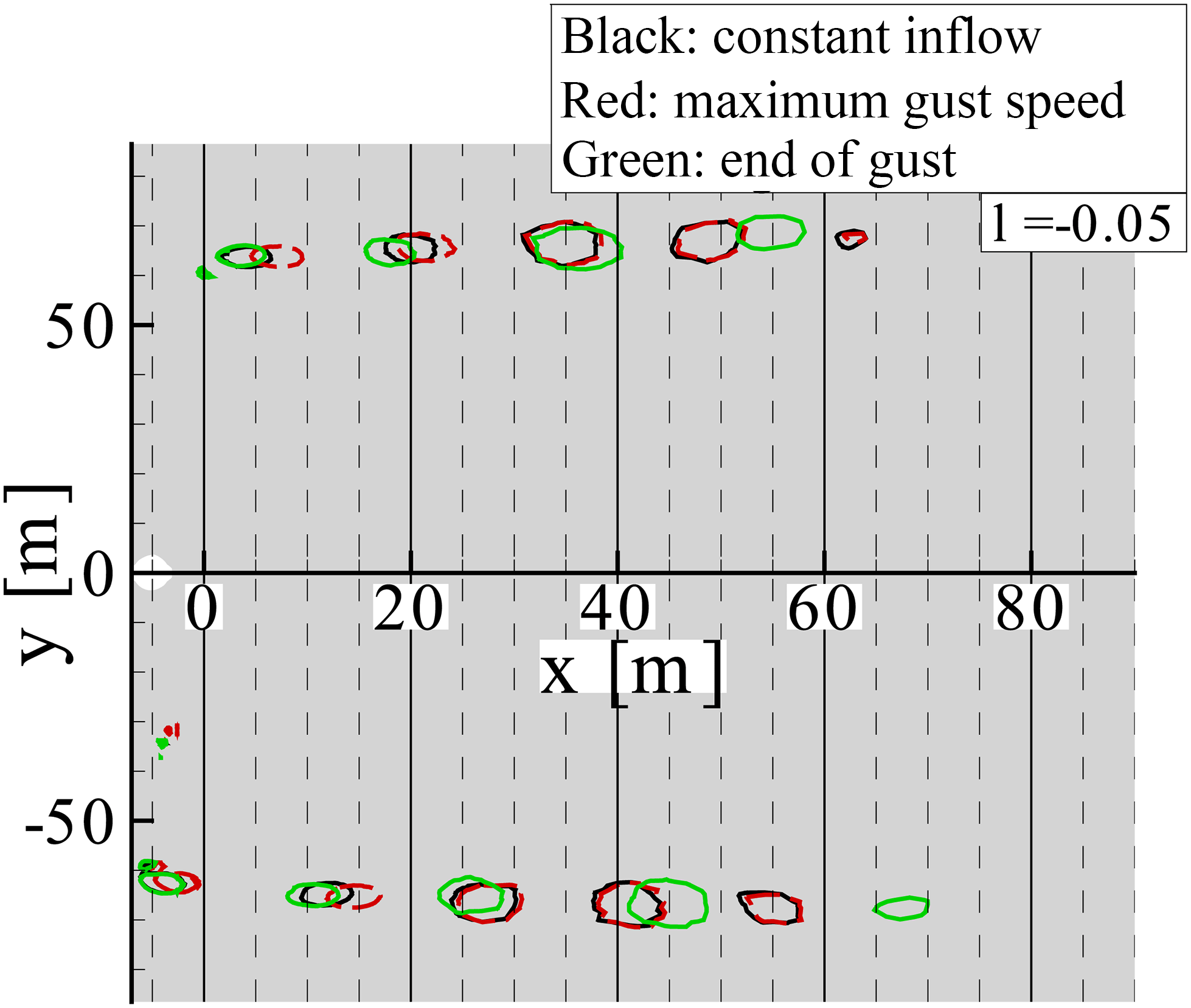
In Fig. 11 three instances of the flow field are compared. In all three instances, the rotor is at the $\mathrm{\Psi }=\mathrm{0}{}^{\circ }$ position. The vortices are made visible with the λ₂ criterion (Jeong and Hussain, 1995). The black lines are extracted during constant inflow, the red lines are extracted shortly before t_max, and the green ones are extracted at the end of the gust. By comparing the vortex transport at the beginning of the gust (black curve) and at the end of the gust (green curve), a compression and stretching of the distance between the vortices is found. The vortex transport with dependence on the vortex age is further discussed through Figs. 12 and 13. They compare the transport of the vortex with dependence on the vortex age parallel and orthogonal to the flow direction, respectively. As long as the inflow velocity is constant, the vortex transport is approximately $\mathrm{0.23}\cdot r/R$ parallel to the flow direction and $\mathrm{0.16}\cdot r/R$ orthogonal to the flow direction in a 1∕3 revolution interval. At maximum gust velocity, the constant distance between the vortices is lost. The vortices older than 1 revolution experienced constant inflow conditions. Thus the inter-vortex distance is constant. The vortices between 0.25 and 1 revolutions were shed during the reduced wind speed. Hence the distance parallel to the flow direction is reduced. As the downstream wake transport decreases, the orthogonal transport increases. The vortices younger than 0.25 revolution experienced the high wind speed. Thus, the distance between the vortices parallel to the flow direction increases and the orthogonal transport decreases. At the end of the gust, reversed behaviour of the vortex transport is observed. The vortices between 0.75 and 1 revolution were generated while the wind speed slowed down. Thus, the distance between the vortices parallel to the wind direction is increased while the orthogonal transport is decreased. Vortices up to an age of 0.75 revolution have a decreased distance parallel to the wind direction but an increased distance orthogonal to the wind direction.

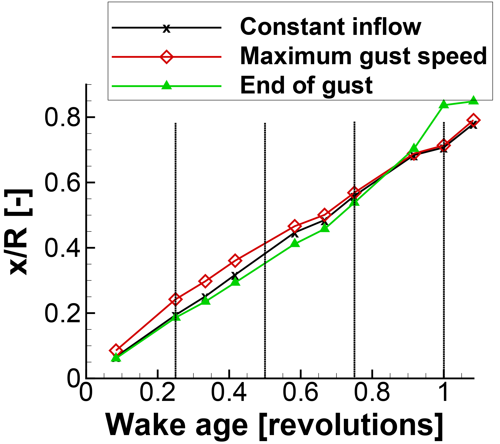
Figure 12 Tip vortex transportation in the main flow direction with dependence on the wake age at three time instances during the gust.

Figure 13 Tip vortex transportation vertical to main flow direction with dependence on the wake age at three time instances during the gust.

The aerodynamic characteristics, rotor thrust, and rotor torque of course depend on the assumption of stiff rotor blades and constant rotational speed. If the rotor had finite mass and inertia or a speed control algorithm had been applied, the rotor loading during the gust would have been reduced significantly. Moreover, the symmetry of the rotor loading decreases as soon as the structure dynamics are taken into account.

6 Conclusions

The study presented the validation of the resolved-gust approach that was implemented in the URANS solver THETA. As a test case, the generic 5 MW wind turbine was computed, operating under a 1−cos() gust and an extreme operating gust as defined in the IEC 61400-1 (2005) standard. The gust has been introduced with the resolved-gust approach (Kelleners and Heinrich, 2015; Reimer et al., 2015) by introducing the changing velocity at the inflow boundary conditions. The gust velocity was then transported loss free through the field with infinite speed of sound. The assumptions made in the paper can be summarized as

1. the wind speed is constant in height and time (except gust velocity);

2. the gust velocity is constant in height;

3. the gust transport velocity is equal to speed of sound which is infinite;

4. the boundary conditions of the flow domain are chosen to prevent the flow from escaping sideways.

The disadvantage of the resolved-gust approach clearly is the requirement of fine time steps and fine grids upstream of the geometry in question, which increases the computational costs. The infinite speed of sound and its direct relation to the gust transport velocity has to be regarded in its ambivalent effects. This leads to an inaccurate reproduction of the wind turbine wake transport on the one hand, while on the other hand, the response of the rotor loading to the gust velocity is immediately obtained. Clear advantages for the resolved-gust approach are numerical stability and no artificial oscillations. Finally, the resolved-gust approach can be applied to any completed wind turbine URANS computation to obtain more insight of the wind turbine characteristics.

The results represented the effects that are expected during the instationary inflow condition in combination with the given boundary conditions very well. Rotor thrust and rotor torque follow the gust shape very closely. An analysis of the time history of rotor thrust and rotor torque during the gust show an increased rotor loading of about 100 % compared to constant inflow. Pressure distributions and friction force coefficients reveal that the flow on the rotor blades at maximum gust velocity is separated and thus highly instationary. Moreover, the effect of accelerating wind speeds was found in the rotor wake as the distance between the vortices is stretched and compressed according to the changes of the wind speed.

The comparison of the results with the aeroelastic software FAST showed a very good agreement of rotor thrust and rotor torque during the EOG. Thus, it is a valid and accurate method to predict wind turbine loads during an EOG. Nevertheless, a complete validation is not possible at this state as a gust experiment for a wind turbine is not available. The first mandatory step for further research on the gust simulation with URANS is to perform a grid-independence and time-step study with the resolved-gust approach. Based on these results, a gust transport velocity with other than infinite speed of sound have to be achieved. This may be realized by adjustments of the resolved-gust approach, by implementing the field approach of, for example, Parameswaran and Baeder (1997), or by implementing the velocity-disturbance approach of Reimer et al. (2015). A third possibility would be to introduce the fluctuating gust velocities obtained from LES computations, which themselves fulfil the continuity conditions. Only then are the procedures of gust computation for wind turbines in THETA prepared to be extended to account for atmospheric boundary layer flows or for aeroelastic analysis. The then ready-to-use method is supposed to supply a tool for gaining more detailed knowledge about the wind turbine behaviour during extreme gust events, in a first step. In a second step, this knowledge can be used to adjust engineering models which are used during the design process. It has to be clearly understood that the resolved-gust approach in an URANS computation cannot and will not replace engineering models at this stage. Consequently, the potential of weight reduction (and thus cost reduction) and increased reliability in wind turbine designs are the (very) long-term objectives.