the Creative Commons Attribution 4.0 License.
the Creative Commons Attribution 4.0 License.
 | 04 Sep 2018
Large-eddy simulation sensitivities to variations of configuration and forcing parameters in canonical boundary-layer flows for wind energy applications
Jeffrey D. Mirocha
Matthew J. Churchfield
Domingo Muñoz-Esparza
Raj K. Rai
Branko Kosović
Sue Ellen Haupt
Barbara Brown
Brandon L. Ennis
Caroline Draxl
Javier Sanz Rodrigo
William J. Shaw
Larry K. Berg
Patrick J. Moriarty
Rodman R. Linn
Veerabhadra R. Kotamarthi
Ramesh Balakrishnan
Joel W. Cline
Michael C. Robinson
Shreyas Ananthan
The sensitivities of idealized large-eddy simulations (LESs) to variations of model configuration and forcing parameters on quantities of interest to wind power applications are examined. Simulated wind speed, turbulent fluxes, spectra and cospectra are assessed in relation to variations in two physical factors, geostrophic wind speed and surface roughness length, and several model configuration choices, including mesh size and grid aspect ratio, turbulence model, and numerical discretization schemes, in three different code bases. Two case studies representing nearly steady neutral and convective atmospheric boundary layer (ABL) flow conditions over nearly flat and homogeneous terrain were used to force and assess idealized LESs, using periodic lateral boundary conditions. Comparison with fast-response velocity measurements at 10 heights within the lowest 100 m indicates that most model configurations performed similarly overall, with differences between observed and predicted wind speed generally smaller than measurement variability. Simulations of convective conditions produced turbulence quantities and spectra that matched the observations well, while those of neutral simulations produced good predictions of stress, but smaller than observed magnitudes of turbulence kinetic energy, likely due to tower wakes influencing the measurements. While sensitivities to model configuration choices and variability in forcing can be considerable, idealized LESs are shown to reliably reproduce quantities of interest to wind energy applications within the lower ABL during quasi-ideal, nearly steady neutral and convective conditions over nearly flat and homogeneous terrain.
- Article
(9511 KB) - Full-text XML
- BibTeX
- EndNote


Accurate characterization and prediction of the microscale wind flow environment plays an important role in many facets of wind power generation, including wind park siting, layout, operations, and the formulation of turbine design standards (e.g., Shaw et al., 2009). While wind power generation has grown tremendously over the last few decades, both turbine reliability and plant power generation frequently underperform projections based on existing turbine design standards and site assessments (e.g., Bailey, 2013). A key contributor to these underperformance issues is the disconnect between the data and models used in turbine and plant design and site assessment, and actual characteristics of the atmospheric boundary layer (ABL), and the in situ wind plant operating environment. Realistic ABL flows under routine atmospheric conditions often include much higher levels of atmospheric turbulence, shear, veer, and other important transient phenomena than are typically captured in measurements or design tools.
Characterization of the wind plant operating environment has historically relied chiefly on observations, typically utilizing a small number of slow-response instruments, augmented occasionally by fast-response instruments capable of accurately characterizing turbulence (Magnusson and Smedman, 1994; Barthelmie et al., 2010). While remote sensing instruments (e.g., Högström et al., 1988; Barthelmie et al., 2003; Nygaard, 2011; Hirth et al., 2012; Rhodes and Lundquist, 2013; Smalikho et al., 2013; Iungo et al., 2013) provide one pathway to improve site characterization, the absence of fast-response turbulence information and limited sampling volumes provided by many systems, coupled with long deployments required to sample long-term variability, constrain the utility of observations for many applications.
Compounding the inadequacies of many observational datasets are the generally lower-fidelity numerical simulation approaches used in conjunction with observations to inform various stages of turbine and plant design and operation. While higher-fidelity simulation techniques exist, their significant computational overhead has precluded widespread adoption due to the limited computational infrastructure generally available to industry (Sanderse et al., 2011; Troldborg et al., 2011).
The increasing availability of high-performance computing infrastructure is enabling more widespread use of high-fidelity numerical techniques, such as the turbulence-resolving large-eddy simulation (LES), to significantly improve understanding of the ABL and wind plant flows. While not yet considered as reliable as established observational and computational approaches, high-fidelity numerical simulations can potentially provide superior site characterization and design data to reduce costs, including (1) flow information over an entire wind farm across many levels within the turbine span, (2) simulation over a distribution of characteristic flow regimes in a short time period, and (3) estimates of flow parameters that are difficult or expensive to observe (e.g., turbulence).
While atmospheric LES is increasingly being utilized to simulate turbulent flows for wind energy applications (Sim et al., 2009; Lu and Porté-Agel, 2011; Bhaganagar and Debnath, 2014; Mehta et al., 2014; Mirocha et al., 2014a; Aitken et al., 2014), by focusing primarily on turbine wakes in quasi-ideal meteorological conditions, these studies have addressed only a limited range of atmospheric conditions and parameters of relevance to industry. Development of atmospheric LES for general meteorological and surface conditions is ongoing; however, this extension relies upon the development of novel forcing treatments both within the computational domain and at the lateral boundaries (e.g., Mirocha et al., 2014a; Muñoz-Esparza et al., 2014, 2015), where assumptions of periodicity and standard approaches for specifying turbulent inflow conditions, such as recycling methods (e.g., Lund et al., 1998; Mayor et al., 2002), precursor simulations (e.g., Churchfield et al., 2012; Mirocha et al., 2014b), or synthetic turbulence generators (e.g., Veers, 1988; Jonkman and Buhl, 2005; Xie and Castro, 2008) are not applicable.
Irrespective of the complexity of the setup, high-fidelity atmospheric LES will require both thorough validation of simulated quantities of interest, and formal assessment of uncertainties, prior to widespread adoption within the wind power industry. To satisfy these requirements, the Atmosphere to Electrons (A2e) initiative within the US Department of Energy's Wind Energy Technologies Office is supporting development and validation of next-generation computational approaches for wind energy applications. This is being undertaken via both assessment of existing simulation approaches, such as idealized LES, and development of new mesoscale–microscale coupling (MMC) methods, as required for extension to more general environments and forcing conditions.
The present study, conducted under the auspices of the A2e MMC project, examines the efficacy of idealized atmospheric LES using periodic lateral boundary conditions (LBCs), an approach commonly applied in fundamental and applied ABL studies (see e.g. Deardorff, 1970, 1980; Moeng, 1984; Kosović and Curry, 2000), to provide flow parameters of interest to wind energy applications. The present study is unique in its focus on the representation of the accuracy of the simulated flow, rather than on turbine interactions, including detailed comparison of simulated and observed turbulence information, including spectra and cospectra. Moreover, we investigate this capability using a computational framework that is both relatively mature and reasonably economical, in comparison with more general yet also more complicated and expensive methods, such as those incorporating time-varying mesoscale input via additional internal forcing terms (e.g. Sanz Rodrigo et al., 2017) or at the lateral domain boundaries (e.g. Muñoz-Esparza et al., 2017; Rai et al., 2017a, b). Finally, an examination of uncertainties provides a required basis for assessment of both existing idealized simulation capabilities, as well as of more sophisticated MMC techniques under development, to the wind energy arena. Section 2 describes the case studies, code bases, boundary conditions, turbulence models, and variations employed to assess uncertainty, Sect. 3 presents simulation results and uncertainty analysis, and Sect. 4 provides a summary and conclusions.
Rather than focusing on turbine response and wake characteristics, as most studies of atmospheric LES targeting wind energy applications have, we instead focus on the accuracy of the resolved atmospheric flow field itself, including profiles of wind speed and direction, turbulence kinetic energy (TKE), turbulent fluxes, and spectra and cospectra. Also included is assessment of simulation uncertainties, undertaken by varying common numerical methods, turbulence models, and setup approaches, using three simulation codes. The simulations are assessed against one another, theoretical expectations, and observations taken from two case studies featuring quasi-ideal ABL flow during nearly steady neutral and convective conditions over nearly flat and homogeneous terrain. The use of quasi-ideal conditions simplifies the attribution of sensitivities to changes of various configuration and forcing parameters representing common simulation setups.
2.1 Case study selection
The Sandia National Laboratories Scaled Wind Farm Technology (SWiFT) test facility, located in the US Southern Great Plains, was selected for the study, due to its nearly flat terrain and homogeneous surface cover, permitting reasonable approximation in idealized computational setups. These setups consist of flat terrain with uniform surface characteristics and forcing conditions, as well as periodic LBCs. Data used to force and evaluate the simulations were obtained from two instrument platforms, a 200 m instrumented meteorological tower, and a radio acoustic sounding system (RASS), each located at the neighboring Texas Tech University's National Wind Institute. The tower provided fast-response data at 10 heights between 0.9 and 200 m from which turbulence and mean flow data were computed, while the RASS data provided an assessment of the prevailing meteorology, as well as estimates of a common parameter used to force atmospheric LES, the geostrophic wind speed, , with ug and vg denoting zonal and meridional components, respectively. Values of ug and vg were estimated using RASS data from above the ABL top, then adjusted slightly until the simulated wind speed and direction profiles above the ABL closely matched the observed values. Other parameters required to force the simulations include the roughness length, z0, which was estimated from the land cover, and fluxes of sensible heat, HS, estimated using values computed from the lowest sensors on the tower, beginning at 0.9 m, and bulk Richardson numbers computed between the 2.4 and 10.1 m measurement heights (see Kelley and Ennis, 2016 for further information about the instrumentation, data processing and site characteristics).
To satisfy conditions under which idealized forcing is appropriate, data were examined for case studies encompassing canonical ABL regimes occurring during convective, neutral, and stable conditions. Criteria for case selection included nearly constant values of wind speed, wind direction, and HS, over time windows of a few hours, with minimal mesoscale variability and influences of moist processes.
Several periods approximating quasi-canonical convective ABL conditions were found within the observational data, with the most ideal, occurring during the apex of solar heating during the early afternoon of the 4 July 2012, selected for the convective case study. In contrast, canonical neutral conditions occurred relatively infrequently, and for much shorter durations, during evening and morning transitions. As transitional boundary layers contain the imprint of preceding stable or convective forcing, many of the candidate neutral periods showed strong influence from prior states and thus were not considered. Furthermore, sonic anemometers on the meteorological tower are mounted on the booms pointing in the west-northwest direction while the dominant wind direction at the SWiFT tower is southerly. As such, most of the candidate neutral cases occurred during times at which the instruments were somewhat influenced by the tower wake. With respect to these constraints, the optimal neutral case study occurred during the evening transition of the 17 August 2012.
While stable conditions are of high importance for wind energy, the combination of difficulties in specifying proper forcing (to capture the correct evolution of the nocturnal low-level jet) and the high computational demands imposed by the fine mesh resolutions required to capture sustained turbulence during moderately stable nocturnal conditions precluded inclusion of a stable case study in the present study.
2.2 Simulation code bases
Three code bases representing standard approaches to ABL simulation are examined.
2.2.1 Weather Research and Forecasting model
The Weather Research and Forecasting (WRF) model (Skamarock et al., 2008) is a community atmospheric simulation framework that supports applications ranging from global to micro scales, including LES, with several subfilter scale (SFS) models available. WRF uses finite differencing to solve the compressible Euler equations, using a split time stepping algorithm within the Runge–Kutta time integration scheme, and a filter for acoustic modes. Advective discretization options include second- through fifth-order in the horizontal and second- or third-order in the vertical.
The WRF model uses a Cartesian mesh, with variables specified on an Arakawa “C” grid. Vertical spacing is specified using a terrain-following pressure-based eta coordinate.
At the model top, WRF imposes free slip for u and v, with vanishing w and fluxes. For the studies herein, the surface shares the same Monin–Obukhov similarity approach as is applied within all three code bases, and described below.
2.2.2 Simulator fOr Wind Farm Applications
The Simulator fOr Wind Farm Applications (SOWFA) (Churchfield et al., 2012) is a collection of flow solvers, turbulence SFS parameterizations, boundary conditions, and utilities for computing wind plant flows. SOWFA is built upon the Open-source Field Operations And Manipulations (OpenFOAM) CFD Toolbox (OpenFOAM, https://openfoam.org/, 2018), a popular, open-source set of libraries for solving partial differential equations. OpenFOAM, hence SOWFA, uses an unstructured-mesh, finite-volume formulation for solving the governing equations. Several options exist for spatial discretization, with second-order central differencing typically used for the advective and diffusive terms. Time advancement is also second-order accurate with Crank–Nicolson implicit discretization. SOWFA's flow solver is Boussinesq incompressible. All variables are located at cell centers, and to avoid velocity–pressure decoupling, a Rhie–Chow-like interpolation of velocity flux to cell faces is used. SOWFA includes Schumann's boundary condition for surface stress and additional boundary conditions for surface temperature flux or cooling rate.
2.2.3 HiGrad
The High Gradient applications (HiGrad) model (Sauer et al., 2016) discretizes the fully compressible, nonhydrostatic Euler equations using the finite-volume technique, on an Arakawa “A” grid. A variety of even- and odd-order advection schemes (first- to fifth-order accurate), as well as two LES SFS models, are available. A third-order explicit Runge–Kutta time-marching method is used in the present study.
2.3 Surface boundary conditions
For all simulations, the surface boundary condition is w=0 with Monin–Obukhov logarithmic similarity theory (Monin and Obukhov, 1954) used to prescribe fluxes of momentum (with moisture ignored in these simulations) as
and heat,
Herein, U is the scalar wind speed, ui are the resolved zonal (i=1) and meridional (i=2) velocity components, z1 is the lowest computed height above the surface, and θS is the surface potential temperature, with , where Pa is a reference value, R is the gas constant for dry air, and cp is the specific heat of dry air at constant pressure. in Eqs. (1) and (2) is the surface–atmosphere exchange coefficient, with z0 the roughness length, and the stability function. During convective conditions, we follow Arya (2001) and Stull (1988) and use , with . Here is the Obukhov length, with , θv0=300 K a reference value of the virtual potential temperature, , where qv is the water vapor mixing ratio, κ=0.4 is the von Kármán constant, and g is the gravitational acceleration. For dry conditions, qv=0 and θv=θ. Due to the interdependence of CD and L during non-neutral conditions, an iterative procedure is applied.
2.4 Turbulence subfilter-scale parameterizations
Four SFS parameterizations were used in the sensitivity analysis (more complete descriptions are available in the references).
2.4.1 Smagorinsky
The Smagorinsky closure (SMAG) (Smagorinsky, 1963; Lilly, 1967) parameterizes the SFS stresses as , where is the eddy viscosity coefficient for momentum, CS is the model constant, is a length scale, and is the resolved strain-rate tensor. Tildes denote resolved components of the flow, with i=1, 2, 3 indicating the velocity components in the x–(u), y–(v), and z–(w) directions, respectively.
Scalar fluxes are given by , with defining the eddy viscosity coefficient for scalar q, and Pr the Prandtl number. Default values utilized herein are CS=0.18 and , with . Modifications applied within WRF and SOWFA during stable conditions are ignored herein.
2.4.2 Lilly
The Lilly model (Lilly) (Lilly, 1967) is similar to the Smagorinsky closure, but uses , with Ce=0.1 the model constant, and e the SFS TKE, obtained via integration of one additional prognostic equation (see code description references for implementation details).
2.4.3 Nonlinear backscatter and anisotropy
The nonlinear backscatter and anisotropy (NBA) model (Kosović, 1997) includes both a linear eddy viscosity component, similar to SMAG and LILLY (but with different values for the constants), and a second term containing nonlinear products of strain rate and rotation rate tensors. The NBA model can be formulated exclusively in terms of velocity gradients or also using e (NBA-TKE), with each dependent upon a single parameter, the backscatter coefficient Cb=0.36 (see above reference for details). As the NBA model specifies only the stresses, which directly determine momentum, turbulent diffusion of scalars uses either the SMAG or LILLY closure, with KM diagnosed from the flow, and used only to compute Kq.
2.5 Simulation setup
Simulations utilized domains of 2.4 km × 2.4 km × 2 km for the neutral case and 6 km × 6 km × 3 km for the convective case, in the x, y and z directions, respectively, with convective conditions requiring larger domains due to deeper ABLs and convective rolls. Constant horizontal grid spacing is used for all simulations. The convective simulations used constant vertical grid spacing throughout, while the neutral simulations used stretching (by 10 % per Δz) for z > 500 m.
While SOWFA and HiGrad use height as the vertical coordinate, WRF's use of a pressure-based coordinate precludes exact specification of heights above the surface; therefore, the heights of the pressure levels are initialized using the hypsometric equation, p(z)= (Holton, 1992), with pS as the surface pressure, R as the dry air gas constant, as the standard atmosphere average temperature over a vertical layer of depth Δz, and z as the grid cell midpoint height value. Subsequent changes to the thermodynamic state of the atmosphere during simulation can cause the heights corresponding to the initial eta values to vary by a few percent over time.
Each simulation utilized damping in the upper portion of the model domain to prevent wave reflection at the model top. WRF utilized Rayleigh damping, which nudges the horizontal wind components toward their geostrophic values, with a coefficient value of 0.003 s−1, and exponentially decreases strength approaching the model top. HiGrad used a similar Rayleigh damping function to that of WRF. SOWFA achieves damping in the upper region of the domain by smoothly transitioning from using purely central differencing of the advective term to a mix of 90 % central and 10 % upwind above a specified height. For all simulations, damping was applied within 400 and 600 m of the model top during the neutral and convective simulations, respectively.
Simulations were initialized with thermodynamic variables approximating observations during the two case studies described previously. Initial horizontal wind components were u=ug, v=vg, and w=0, with potential temperature profiles of. Here, , where p0=1000 hPa is a reference pressure, θB is a background constant value, a(z) specifies an inversion, to prevent turbulence from reaching the model top, and a′(z) are small perturbations , drawn from a uniform distribution, and scaled as a decreasing cubic function of height from the surface. These small perturbations are applied only to the initial condition to seed turbulence. The neutral simulations used θB=300 K, with the termination of the perturbations and base of the inversion specified at 500 m, with an inversion strength of 10 K km−1. The convective simulations used θB=309 K, with perturbations up to 400 m, and an inversion beginning at 600 m, with a strength of 4 K km−1. SOWFA, which uses temperature rather than θ, specified the initial temperature to be consistent with θ, as described above. WRF and HiGrad specified a hydrostatic base state pressure distribution using the above described θ distribution and pS=P0. SOWFA, which uses an incompressible solver, and therefore requires no background pressure (only gradients of pressure are resolved), added a background value of p0 to the computed pressure field, to be consistent with the other solvers.
For these idealized simulations, which were based upon case studies with no precipitation, and little cloudiness or synoptic-scale weather variability, the simulations were initialized dry, and the only physical process parameterizations utilized were SFS turbulence fluxes, with surface sensible heat and stresses as described in Sect. 2.3.
Due to the initial flow field being nonturbulent and not in balance with the applied geostrophic forcing, a spin-up period was required for the flow statistics to approach nearly steady values. During neutral conditions, the spin-up period is longer, due to the weak turbulence forcing, and the existence of an inertial oscillation with a period of several hours (at the specified latitude of 33.5∘). As differences in model formulation, resolution, and SFS model all influence the period of the inertial oscillation, via impacts on turbulent transport, the simulations were compared during the 2 h surrounding the point in time in which each simulation reached its first maximum in the planar, 10 min average horizontal wind speed at 80 m above the surface. The time of occurrence of the first wind speed maximum varied between 11 and 15 h following initialization, depending on model configuration and forcing. While the flow had not equilibrated completely, this methodology allowed for comparison at the same point in the evolution of each simulation. Further, wind speed values at 80 m varied by only a few tenths of a m s−1 over the period spanning the peak, yielding minimal impacts on quantities of interest. Continuing the simulations further in time would have achieved only negligible changes at the expense of reducing the number of configurations examined, given the high computational expense of each simulation.
For the convective case study, which requires much shorter spin-up due to strong buoyant forcing dominating turbulence and ABL characteristics, the model solutions were compared after 1 h.
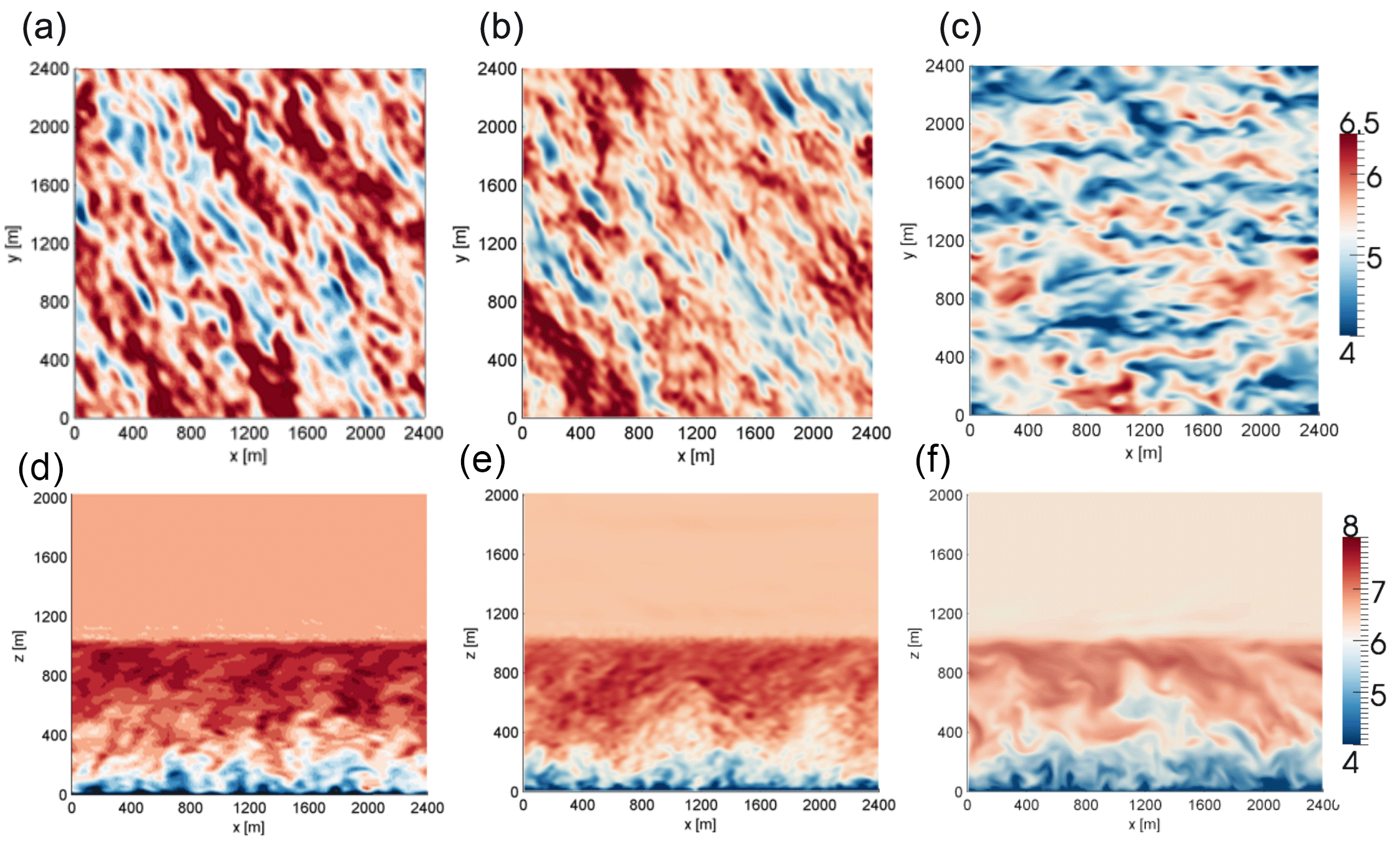
Figure 1Comparisons of instantaneous horizontal wind speed [m s−1] from the neutral case study, at 100 m above the surface (a, b, c) and in a cross-stream plane midway through the domain (d, e, f) from WRF (a, d), SOWFA (b, e) and HiGrad (c, f). In each case, the external forcing was the same, grid resolution was 15 m in each direction, and the advective scheme was the lowest-order option for each solver.
2.6 Sensitivity experiments
Sensitivities of the simulations to variability in model forcing, numerical methods, configuration, and turbulence SFS models were obtained from a suite of simulations using different values of relevant parameters. Sensitivity to forcing was examined by varying Ug and z0 around estimated base values (as described in Sect. 2.1) during the neutral case study, and using two representative values of HS, with Ug and z0 values held constant, during convective conditions). Configuration parameters included mesh resolution in the vertical (Δz) and horizontal (Δx=Δy) directions, the combination of which determine two other parameters that impact model performance, the grid aspect ratio, , and l. Vertical and horizontal mesh resolutions were therefore varied independently to isolate sensitivities to each. Sensitivity to different orders of accuracy of advection schemes in both horizontal, O(h), and vertical O(v), directions, was also examined.
While forcing and configuration parameters could be varied within all code bases, not all codes supported multiple options for all parameters. The sensitivity experiments therefore involved changes both across and within the different codes. Due to the large number of parameters, assessing the impacts of each independently was infeasible. Instead, forcing, configuration, numerics, and SFS turbulence options were combined into a large yet feasible suite of simulations listed in Tables 1–2 (the * symbol in the SOWFA simulations indicates reductions of the model constants, to CS=0.135 and Ce=0.0673, the latter resulting in an effective CS value of 0.135; see Sullivan et al., 1994). While results from all setups in Tables 1–2 were analyzed, for brevity only a subset is presented herein.
Table 1Forcing and configuration parameters for the neutral-case sensitivity studies, using WRF (W), SOWFA (S), and HiGrad (H), as described in the text.
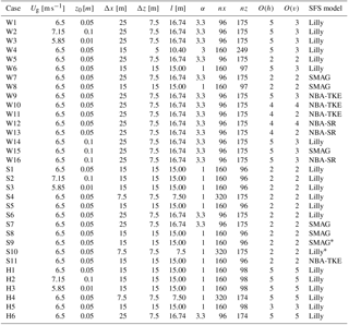
Table 2Forcing and configuration parameters for the convective-case sensitivity studies, using WRF (W), SOWFA (S), and HiGrad (H), as described in the text.
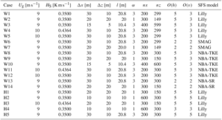
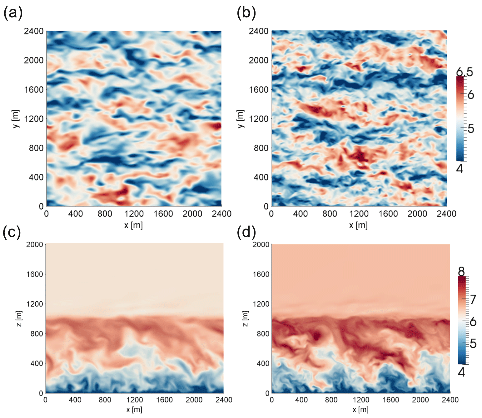
Figure 2Comparisons of instantaneous horizontal wind speed [m s−1] from the neutral case study, at 100 m above the surface (a, b) and in a cross-stream plane midway through the domain (c, d). From the HiGrad solver operating at a 15 m resolution in each direction and using order 3 advective discretization (a, c), and a 7.5 m resolution in each direction and order 5 advective discretization (b, d).
3.1 Qualitative assessment
First, high-level results from the sensitivity simulations are shown to indicate some key differences between the case studies and solvers. A more detailed comparison of various flow parameters from the simulations is provided in Sect. 3.2.
3.1.1 Neutral case
Figure 1 shows instantaneous horizontal wind speed in both x–y cross-sections at 100 m above the surface (top) and in vertical x–z cross sections at the y-direction midpoint (bottom), from all three solvers. The same forcing is used for all simulations, with the exception being the geostrophic wind direction, which was set to westerly in the HiGrad simulations, rather than northwesterly in WRF and SOWFA. Due to the idealized setup, using flat terrain, homogeneous surface and atmospheric forcing, and periodic LBCs, the only effect of this difference is to rotate the simulated wind direction, with no impacts on relevant flow characteristics. Each simulation used a grid resolution of 15 m in all directions, with the discretization of the advective term the lowest order option, , in WRF and SOWFA, and 3 in HiGrad.
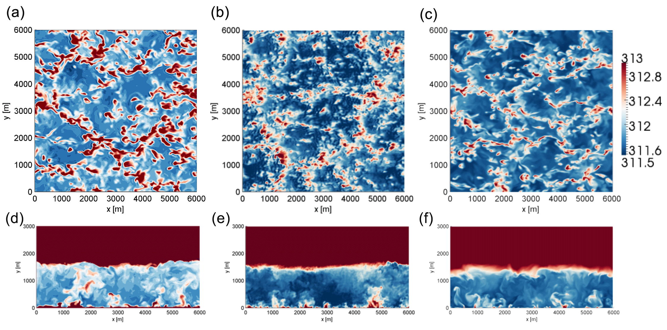
Figure 3Comparisons of instantaneous potential temperature [K] from the unstable case study, at 100 m above the surface (a, b, c) and in a cross-stream plane midway through the domain (d, e, f) from WRF (a, d), SOWFA (b, e), and HiGrad (c, f). Each simulation used the same external forcing but different solver options, as described in the text.
While differences among the solutions are apparent, all three solvers show similar characteristic turbulence structures, namely the elongated low-speed streamwise structures, a range of sizes of turbulence structures, diminishing with increasing proximity to the surface, and similar ABL heights, due to the capping inversion.
Figure 2 shows the impacts of increasing both the grid resolution and the accuracy of the advective operators within the same solver, in this case HiGrad, on instantaneous wind speed, in the same two planes as Fig. 1. The grid spacing was decreased by a factor of two in all directions, while O(h) and O(v) were increased from three to five. Results of these changes include a broader range of flow structures, particularly at the small-scale end of the spectrum, due to more of the inertial subrange being explicitly resolved, as well as the wider range of magnitudes, with both lower minima and higher maxima within the resolved structures. Similar impacts were observed for all three solvers under corresponding changes to grid resolution and advection schemes (not shown).
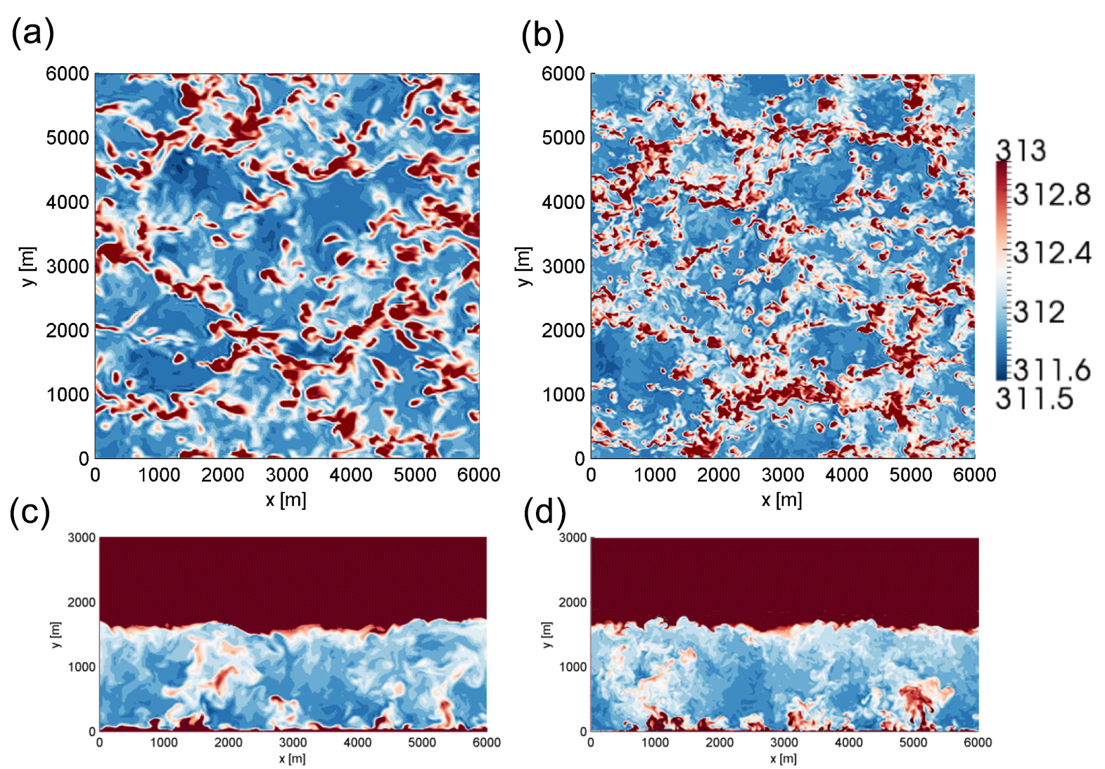
Figure 4Comparison of instantaneous potential temperature in the convective case at 100 m above the surface (a, b) and in a cross-stream plane midway through the domain (c, d) from the WRF solver operating at a 30 m horizontal by 10 m vertical resolution (a, c) and a 15 m horizontal by 5 m vertical resolution (b, d).
3.1.2 Convective case
Figure 3 shows instantaneous cross sections of potential temperature in both the x–y plane at 100 m above the surface (top), and the x–z plane at the domain y-direction midpoint (bottom), from the convective case study, using the WRF (left), SOWFA (middle), and HiGrad (right) solvers, as in Fig. 1. Each of the simulations shown in Fig. 3 used identical physical forcing (Ug, HS, and z0); however, different numerical settings and grid configurations were employed. With near-surface flow parameters showing strong sensitivity to the value of α near the surface in previous LES studies (Brasseur and Wei, 2010; Mirocha et al., 2010; Ercolani et al, 2017), each simulation shown in Fig. 3 utilized the α value that produced the best agreement with the expected logarithmic similarity solution in the surface layer within that solver base; for SOWFA and HiGrad, and for WRF. Therefore, the HiGrad and SOWFA simulations shown in Fig. 3 use an isotropic grid with α=1 and with grid cell sizes of 20 m in each direction, while WRF uses α=3, with horizontal and vertical grid spacings of 30 and 10 m, respectively. To compensate for the coarser horizontal resolution, the WRF simulation used its highest-order advection options, O(h)=5 and, O(h)=3, while the lowest-order options, 2 and 3, were used for SOWFA and HiGrad, respectively.
Inspection of Fig. 3 reveals qualitative similarities in resolved flow characteristics, including the shapes and sizes of the turbulent structures in both cross sections. However, the WRF simulations exhibit less fine-scale structure than the others, despite the use of higher resolution in the vertical direction, and higher-order advection operators, indicating that horizontal resolution is the dominant factor influencing the size distribution of resolved scales, within the examined range of parameter values. The slightly higher temperatures within the WRF ABL (Fig. 3) are most likely artifacts of the Rayleigh damping imposed above the ABL, which relaxes temperature back to its initial value beginning at the ABL top. WRF also generates a slightly deeper ABL, likely due to a combination of higher vertical resolution and a warmer ABL, the latter slightly reducing the relative strength of the capping inversion. HiGrad produces the shallowest ABL, despite using the same resolution as SOWFA, likely due to its use of an odd-order advection operator, which being more dispersive than SOWFA's even-order operator, slightly reduces TKE (see Fig. 16a).
Figure 4 isolates the impact of changing only the mesh resolution (by a factor of three in each direction) within the same solver (WRF) while leaving all other settings constant. Instantaneous cross sections in the same two planes as shown in Fig. 4, from the coarse-resolution (left) and fine-resolution (right) simulations, show that while both resolutions capture the same morphological characteristic, most notably quasi-cellular convective cells of similar sizes and magnitudes, an increased range of scales of motion are captured with the finer-resolution LES.
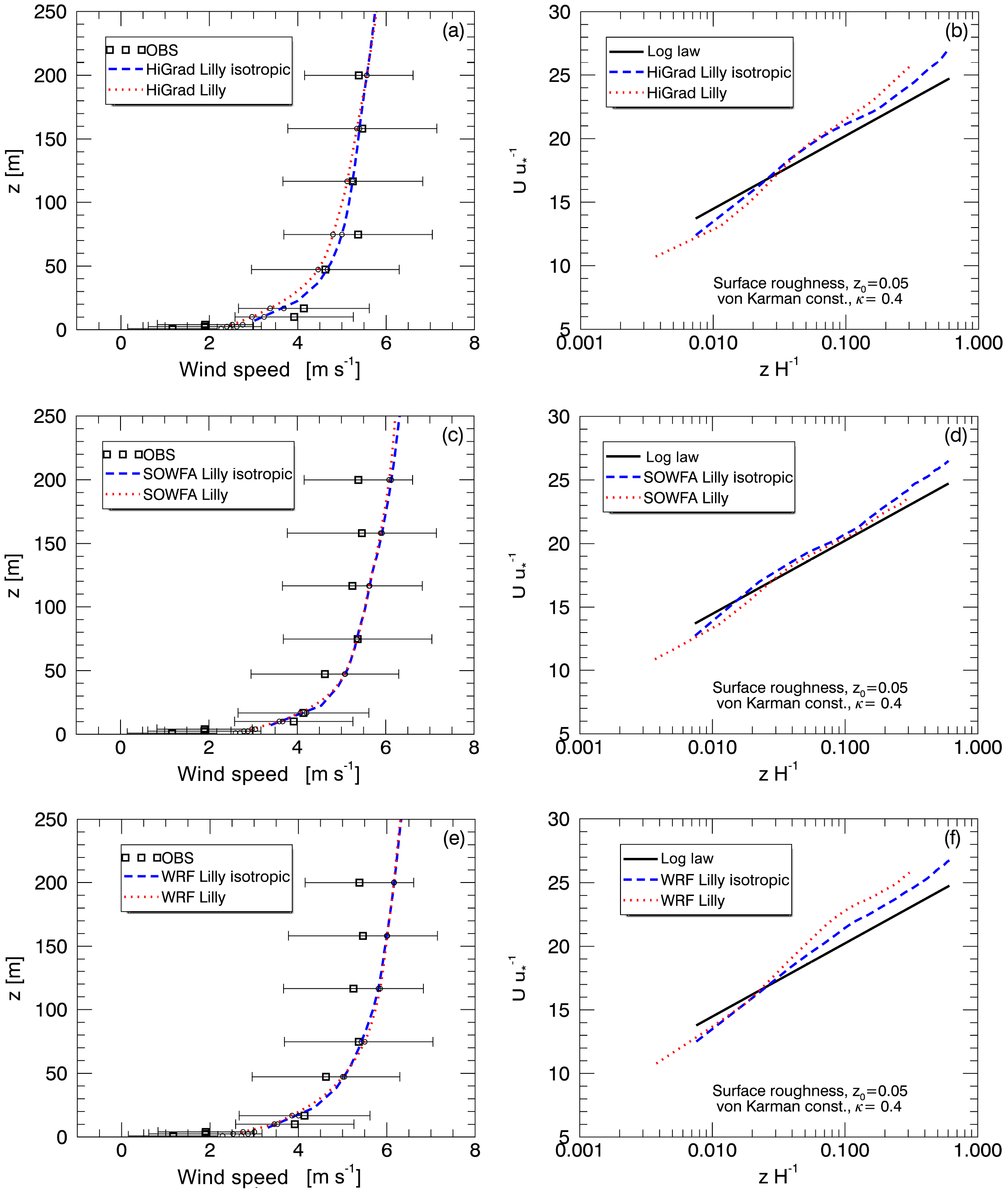
Figure 5Simulated profiles of time-averaged wind speed plotted against observations (a, c, e) and the theoretical logarithmic profile shape (b, d, f), from the neutral case study, using HiGrad (a, b), SOWFA (c, d), and WRF (e, f).
3.2 Quantitative assessment
The ABLs and simulations thereof comprising this study are approximately horizontally homogeneous; therefore averaging over horizontal planes could be applied for assessment. However, considering that future planned studies will involve heterogeneous boundary layers under time-varying forcing, temporal averaging and spectral analysis in the frequency domain is instead utilized. Simulation results therefore consist of a single vertical profile located near the center of the computational domain, which is output every second (1 Hz) during the time window of analysis.
3.2.1 Neutral case
As described in Sect. 2.1, the evening transition of the 17 August 2012 provided the best approximation to canonical near neutral ABL conditions within the observational dataset; however, subsequent detailed analysis of TKE measured with sonic anemometers at the SWiFT tower showed that the instruments were partially in the wake of the tower. This resulted in larger measured TKE values than what would be expected in unobstructed flow under the same conditions. As the tower cross section and lattice structure comprise length scales much smaller than the characteristic production scales of turbulence for the considered ABL types, most of the covariance, arising primarily from the largest eddies, is hypothesized to have been only minimally impacted by the tower. Therefore, while preventing a detailed comparison of TKE, other parameters not strongly impacted by the quasi-random perturbations created by tower interactions, such as turbulent stresses and velocity spectra and cospectra, were compared qualitatively. Mean wind speed and direction profiles, which showed no evidence of tower wake influence, were compared quantitatively.
Sensitivity to model configuration
Figure 5 shows time-averaged profiles of wind speed from simulations using all three solver bases, compared against both measurements at the SWiFT tower (left), and to the theoretical logarithmic profiles in the surface layer (right). Measurement variability is shown as “uncertainty” bars that signify one standard deviation from a mean value computed as a 90 min time average. All simulations use the Lilly SFS model and the highest-order advection option available. Two different grid setups were used, with horizontal and vertical grid sizes of 25 and 7.5 m for WRF, resulting in α=3, and 15 m each for SOWFA and HiGrad. This in turn resulted in α=1, yielding optimal performance for each model, as described in Sect. 2.6.
Despite the use of different numerical and grid specifications, all simulations produced generally good agreement with measurements, falling within measurement variability. The measured wind speed profile does not increase monotonically with height, as would be expected in canonical ABL flow, indicating the presence of height-dependent transient processes and forcings. Considering that such processes cannot be captured with idealized forcing and simulation setups, the agreement between the model output and the data can be considered to be quite good. The logarithmic profile in the surface layer is also captured well, despite the known tendency of the Lilly SFS parameterization to overpredict nondimensional shear relative to a logarithmic profile in the surface layer of a neutral ABL (Brasseur and Wei, 2010; Mirocha et al., 2010).
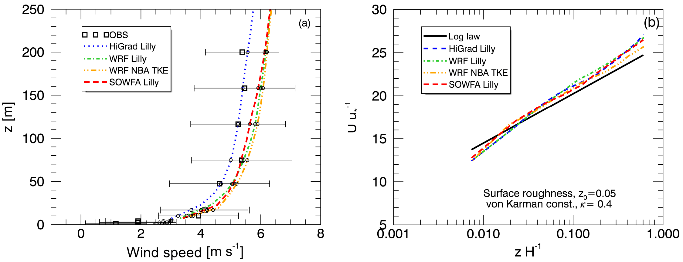
Figure 6Impacts of different solvers, all using isotropic grids of 15 m in each direction, on simulated profiles of time-averaged wind speed plotted against observations (a) and the theoretical logarithmic profile shape (b), from the neutral case study.
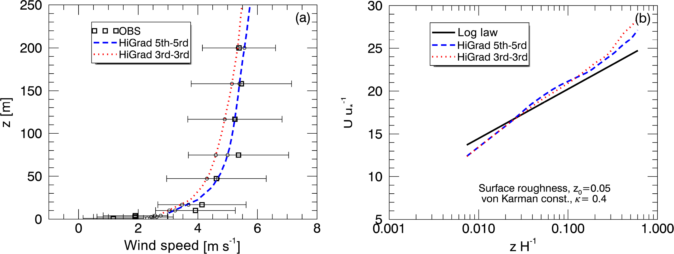
Figure 7Impacts of different advection schemes within the HiGrad model, on simulated profiles of time-averaged wind speed plotted against observations (a) and the theoretical logarithmic profile shape (b), from the neutral case study.
Figure 6 compares simulated wind speed profiles using the three models, all with isotropic grid formulations, while also showing the impact of using two different SFS parameterizations in WRF, Lilly, and NBA-TKE. Again, results are generally similar, with HiGrad showing slightly slower wind speeds above 50 m, slightly closer to the mean of the observations, than SOWFA and WRF. All models reproduce logarithmic near-surface shear profiles reasonably well (Fig. 6b).
The impact of different advection operators was also analyzed. Here, only results from HiGrad and WRF are presented, as SOWFA includes only one advection option. Figure 7 shows results from HiGrad with and five upwind advection schemes, indicating better agreement with measurements using higher-order schemes. Figure 8 shows the impact of different combinations of advective scheme and SFS stress model (Lilly and NBA) on WRF's wind speed profiles, indicating that, for this suite of simulations, either configuration choice results in variability of similar magnitude.
The relative performances of various configurations are assessed quantitatively using the mean absolute error (MAE), root mean square error (RMSE), and vertical shear, computed across two different depths. Tower MAE and RMSE were computed across all heights on the tower spanned by the model mesh (no extrapolation to tower values below the lowest model height), by interpolating model values to the sensor heights using cubic splines. Rotor MAE and shear were computed analogously over a depth of 40 to 140 m, corresponding to the swept area of a representative modern utility-scale wind turbine with a 100 m rotor diameter and a hub height of 90 m. Wind profile characteristics within and across the rotor swept area are relevant to both power production and fatigue loading.
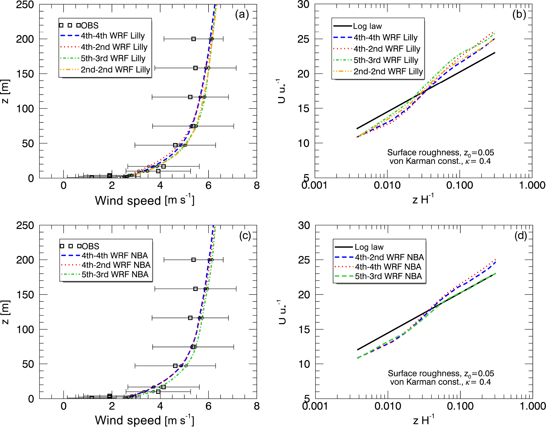
Figure 8Impacts of varying advection schemes and SFS models in WRF, on simulated profiles of time-averaged wind speed plotted against observations (a, c) and the theoretical logarithmic profile shape (b, d), from the neutral case study. Simulations used Lilly (a, b) and NBA (c, d) SFS parameterizations.
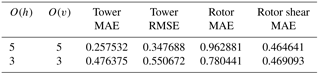
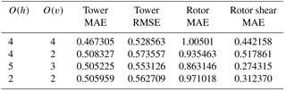
Table 3 shows the impact of varying the order of the advective operators within the HiGrad model on each of the above statistics, indicating that changes to this configuration choice result in generally small changes in velocity profile characteristics across both the tower and the rotor, with neither the higher- nor lower-order results notably superior overall.
Table 3Analysis of HiGrad performance using different advection schemes with the Lilly SFS parameterization.
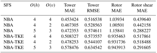
Similar analysis was performed using the WRF model varying the order of the advection scheme and the SFS parameterizations, as summarized in Tables 4 and 5. Here, O(h)=3, 4, and 5 were used in horizontal, and O(v)=2 and 3 in the vertical directions. These advection schemes were varied in combination with the Lilly, NBA, and NBA-TKE SFS parameterizations. Tables 4 and 5 show that using different advection schemes results in variability of comparable or even greater magnitude than that resulting from different SFS parameterizations, with no choice clearly superior in all metrics.
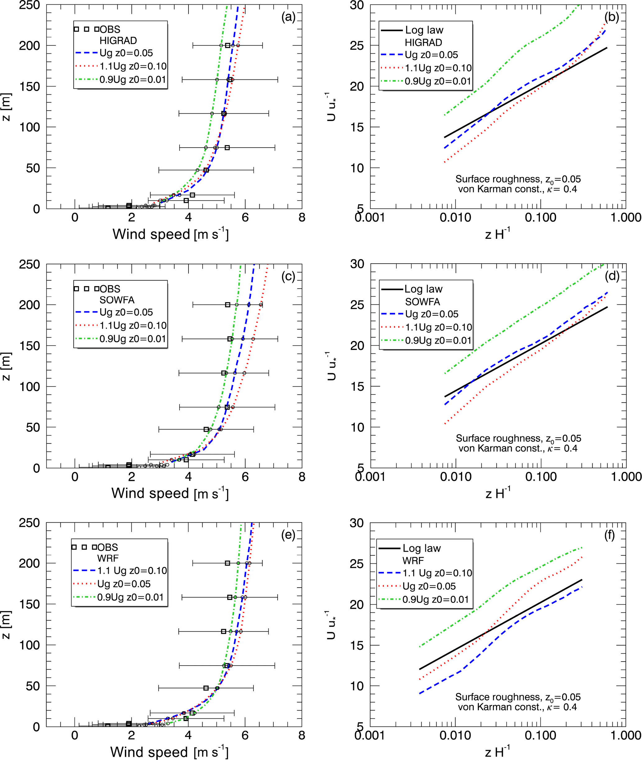
Figure 9Impacts of varying surface roughness length and geostrophic wind speed using HiGrad (a, b), SOWFA (c, d), and WRF (e, f), on simulated profiles of time-averaged wind speed, plotted against observations (a, c, e) and the theoretical logarithmic profile shape (b, d, f), from the neutral case study.
As numerical simulations of homogeneous boundary layers generally represent ideal conditions, more realistic simulations may include significant spatial gradients associated with, for example, microfronts. For such applications, odd-order upwind schemes would likely be advantageous. The analysis of WRF results indicates that the choice of the advection scheme could be as important as the choice of a SFS parameterization and that the best performance is obtained with specific combinations of SFS parameterizations and advection schemes (also see Fig. 8).
Table 4Analysis of WRF LES performance using different advection schemes with the Lilly SFS parameterization.
Sensitivity to forcing parameters
Assessment of sensitivity to two key boundary conditions and forcing parameters, z0 and Ug, is also performed. Each of these parameters is typically held uniform in space and constant in time in idealized LES, and therefore must represent average values. The baseline values for these parameters, z0=0.05 m and m s−1, were bracketed by two additional cases, z0=0.01 m and , and z0=0.1 m and . The wind speed profiles resulting from changes of these parameters in all three models are shown in Fig. 9, indicating that each model exhibits the expected behavior of increasing wind speed at upper measurement levels of the SWiFT tower when Ug is increased (Fig. 9, left).
The effects of varying z0 are better seen by comparing surface layer wind speed profiles with the logarithmic profiles shown in panels on the right of Fig. 9. While all profiles appear nearly logarithmic, each model generates a slightly different slope of the wind speed profile near the surface, with simulations using the smaller z0values showing smaller departures from the baseline profiles than those using increased values, due to the z0 value being a factor of five smaller, versus only a factor of two larger, in the reduced and increased value cases, respectively.
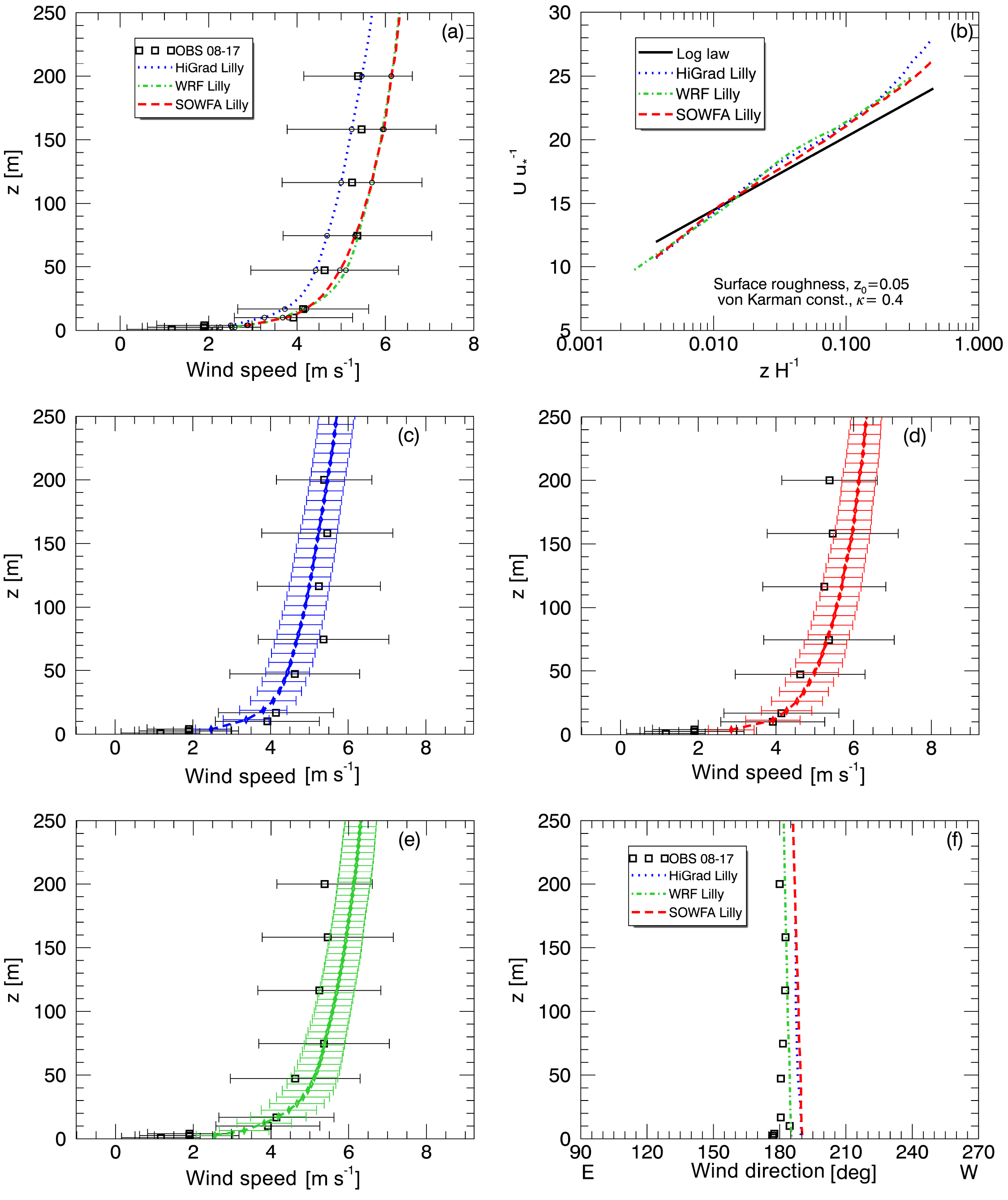
Figure 10Observed and simulated wind speed and direction, from the neutral case study, using higher resolution, with each solver using its optimal aspect ratio and the Lilly SFS model. Top panels show each models' mean wind speeds against observed variability (a, c, e) and the theoretical logarithmic distribution (b, d, f). Middle and lower panels show each models' mean and variability relative to the observations, with wind direction shown in the lower right.
Differences in response to varying surface boundary conditions among the models can likely be attributed to differences in implementation of surface boundary conditions. Considering the infeasibility of resolving the viscous sublayer of a high-Reynolds-number ABL flow, due to both extreme computational demands and uncertainties in details of terrain and surface cover, LES of ABLs generally rely on approximate surface boundary conditions that are in some form based upon the assumption of a developed logarithmic surface layer profile, modified by atmospheric stability (e.g., Moeng, 1984).
Assessment of high-resolution simulations
The preceding analysis of sensitivity to model configuration and forcing parameters utilized simulations conducted with moderately fine grid resolutions. A more detailed assessment of model performance based on higher-resolution simulations of the baseline case of z0=0.05 m and m s−1 was also conducted. Each of the higher-resolution simulations was configured according each model's optimal α value, with HiGrad and SOWFA using an isotropic grid with α=1, and grid cell sizes of 7.5 m in each direction, while WRF used α=3, with horizontal and vertical grid spacings of 15 and 5 m, respectively. To maintain the same domain size, HiGrad and SOWFA used grid cells in the x, y, and z directions, while WRF used , respectively. All simulations used the Lilly SFS model.
A comparison of simulated and observed time-averaged wind speed profiles is shown in Fig. 10a. Excellent agreement is observed between SOWFA and WRF model results, each predicting slightly higher magnitudes than HiGrad, with all simulations falling within the range of observed variability. Each simulation also produced good agreement with the logarithmic profile in the surface layer (Fig. 10b). Temporal variability of the 10 min average wind speed for each simulation is shown in Fig. 10c, d, and e, denoted as “error” bars, representing one standard deviation from the mean across all 10 min averages. All three models result in similar temporal variability, all markedly lower than that of measured profiles. The difference between simulated and measured variability could be attributed to the fact that idealized simulations forced with constant and uniform Ug did not account for possible variability in large scale forcing that could be associated with the evening transition. Also, the SWiFT tower wake effects, as described in Sect. 3.2.1, have likely artificially enhanced velocity variations. Moreover, simulated variability was calculated using only resolved velocity fluctuations, ignoring the SFS component which may have further increased the range of variability from the simulations.
For completeness, comparison between measured and simulated wind direction is shown in Fig. 10f. Excellent agreement is observed except for a small difference at the lowest levels that could be potentially attributed to the effects of small terrain heterogeneities not represented within the simulations.
Table 5Analysis of WRF LES performance using different advection schemes with the NBA and NBA-TKE SFS parameterization.
Quantitative MAE and RMSE values from the high-resolution simulations are presented in Table 6. While all the models perform well, the HiGrad simulations produce the lowest values of wind speed MAE and RMSE across the tower depth, as well as the lowest value of wind speed MAE across the rotor heights. The SOWFA simulations achieve the lowest shear MAE across the rotor disk. It is noted that configurations used for the high-resolution simulations may not have been optimal for each model. As discussed earlier, using model configurations with different combinations of SFS models and advection schemes may yield better performance. In addition, uncertainty in the forcing conditions and the unsteadiness of the evening transition may have contributed to these errors. Finally, WRF's relatively lower scores are likely partially attributable to the use of a factor of two coarser horizontal resolution (relative to the other models), a key modulator of resolved turbulence scales.
Table 6Analysis of high-resolution LES performance using different models with the Lilly SFS parameterization for the neutrally stratified ABL observed on 17 August 2012.
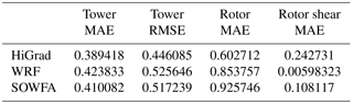
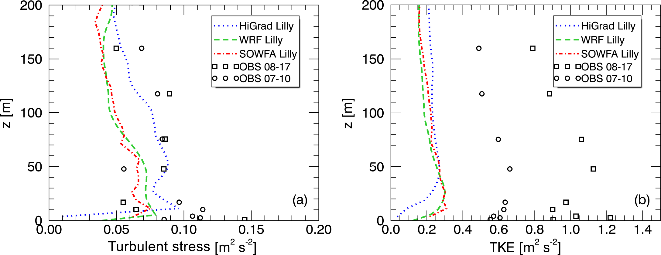
Figure 11Simulated and measured turbulent stress (a) and TKE (b), from the neutral case study.
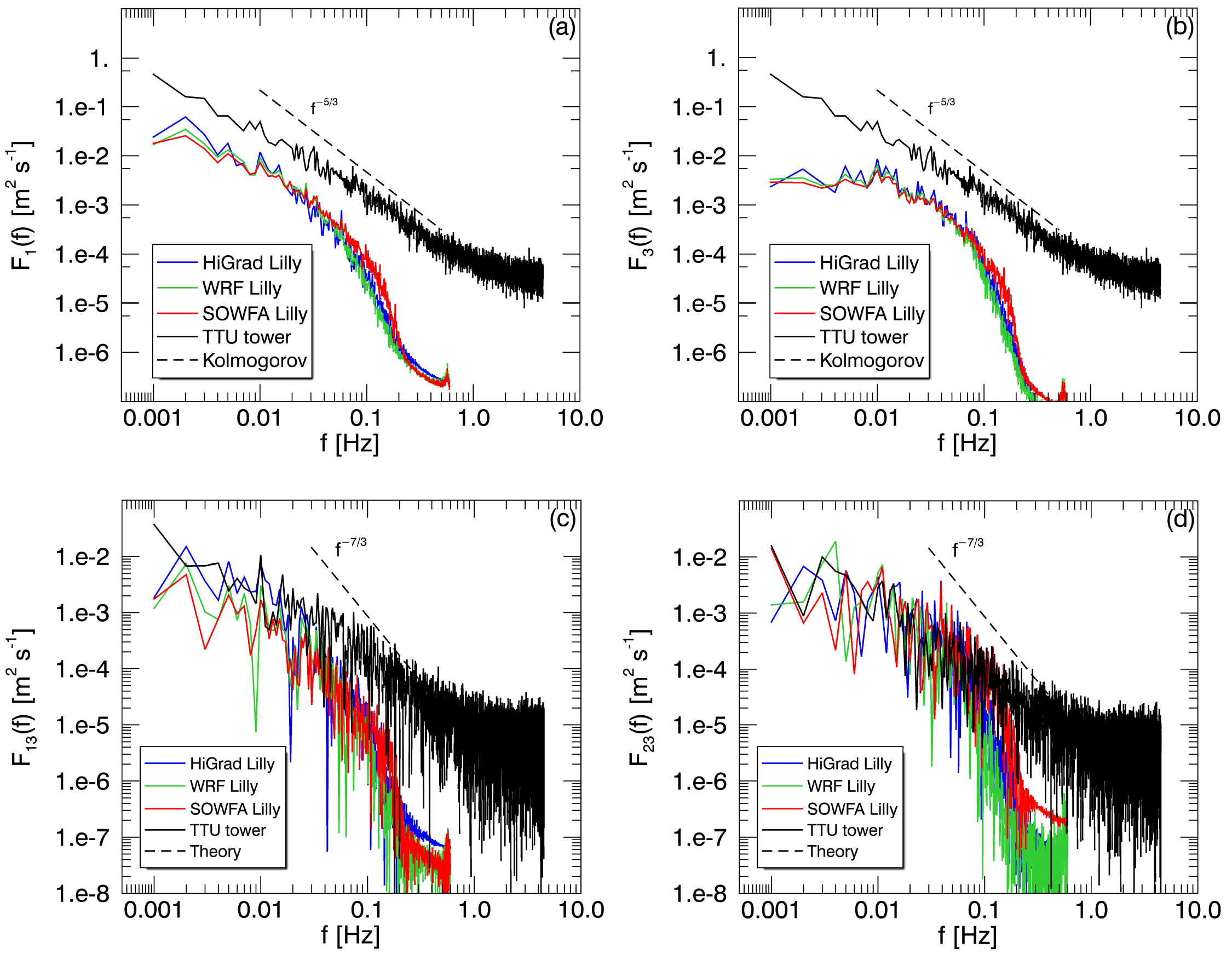
Figure 12Simulated and measured spectra of the streamwise (a) and vertical (b) velocity, and cospectral components Co (c) and Co (d), from the 17 August neutral case study, at 80–90 m above the surface.
In addition to wind speed and direction, time-averaged profiles of vertical turbulent stresses, with and , and TKE , were also examined. Here a′ represents an instantaneous deviation from an average value, with 〈a〉 representing the averaging. Measured values of stresses and TKE were computed from tilt-corrected and detrended high-rate (50 Hz) measurements, while simulated values used a 1 Hz output, and include both resolved and SFS components. Measurements were subsampled to 1 Hz to match the simulation output.
Figure 11 shows time-averaged turbulent stresses (left) and TKE (right) from both simulations and observations. All quantities were computed over a 90 min period using 15 min running mean values. In addition to the 17 August case, observations here include an additional near-neutral period occurring during the morning of the 10 July 2012, which featured similar but slightly greater wind speeds (by approximately 1 m s−1 over the depth of the tower), but from a different direction that avoided tower wake contamination. Agreement between the magnitudes of the simulated and observed stress is generally good, with similar values observed during both periods. Simulated TKE values, however, are significantly smaller than observed values during both periods, with observed magnitudes also differing substantially between the two periods.
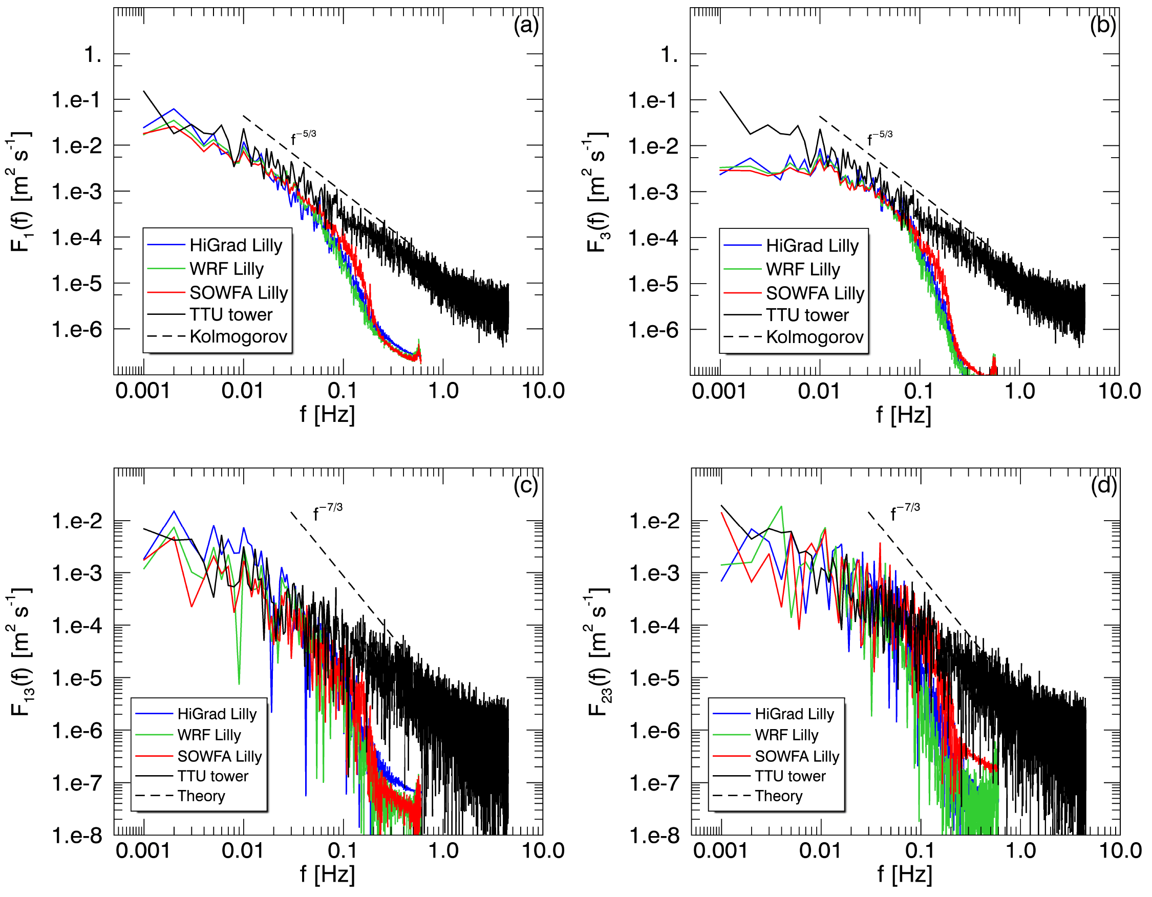
Figure 13Simulated and measured spectra and cospectra, as in Fig. 12, from another neutral case study occurring 10 July 2012, exhibiting no tower wake effects.
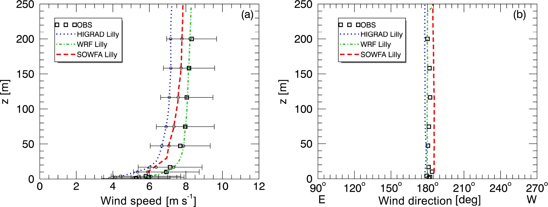
Figure 14Measured and simulated wind speed (a) and wind direction (b) using all three solvers, each with its optimal aspect ratio, during the convective case study.
An explanation for the large differences between measured and observed TKE values, despite similar stress values, is that tower wake effects likely contributed small, uncorrelated perturbations, enhancing the variances contributing to TKE while not strongly impacting the covariances that determine the stress. The larger observed TKE values during the unwaked 10 July case are likely due to greater vertical wind shear occurring within the stable conditions preceding the near neutral morning transition period. Observed TKE values during the 17 August case also could have been influenced by residual turbulence from the previous afternoon's convection. These factors highlight difficulties inherent in comparing observations taken during near-neutral periods within a diurnal cycle, to idealized neutral simulations forced with no diurnal variability. Despite the omission of diurnal variability (and other simplifications) in the idealized setups used herein, the stress values, which are critical factors in turbine fatigue loading, were captured well.
Figure 12 shows power spectra of streamwise (top left) and vertical velocity (top right) components, as well as cospectra of two turbulent stress components: and . All spectra and cospectra are computed at a representative wind turbine hub height between 80 and 90 m, but at slightly different heights due to differences between the grid-cell height values of the simulations and the tower instrumentation. Values were computed from the 1 Hz data and model output by dividing a 90 min time series into overlapping 15 min intervals (overlapping over 7.5 min) and averaging the resulting 11 spectra and cospectra.
The spectra shown in Fig. 12 (top) suggest that the primary cause of the larger measured than simulated TKE values is increased variability in the observed horizontal velocity components relative to the simulations, likely due to tower wake effects. In contrast, the cospectra (bottom) show much better agreement between simulations and observations due to their dependence upon correlated structures produced by nonlinear dynamics, rather than the generally uncorrelated structures produced by the lattice tower.
Spectra and cospectra computed from model output display a high-wave-number drop-off characteristic of finite difference and finite volume discretization schemes. A numerical scheme without full spectral resolution acts as a low-pass filter with a width that depends on the type and order of the numerical scheme (Kosović et al., 2002; Skamarock, 2004). As can be seen from Fig. 12, all three models exhibit similar high-wave-number drop-off characteristics, as expected, with the SOWFA results producing slightly wider inertial subranges due to the use of an even-order, centered scheme.
Figure 13 shows velocity spectra and cospectra, as in Fig. 12, from the unwaked 10 July case. As with the 17 August case, observed and simulated cospectra and vertical velocity spectra again agree well with each other. However, the absence of spurious, tower-induced horizontal velocity perturbations greatly improves agreement between the measured and simulated horizontal velocity spectra.
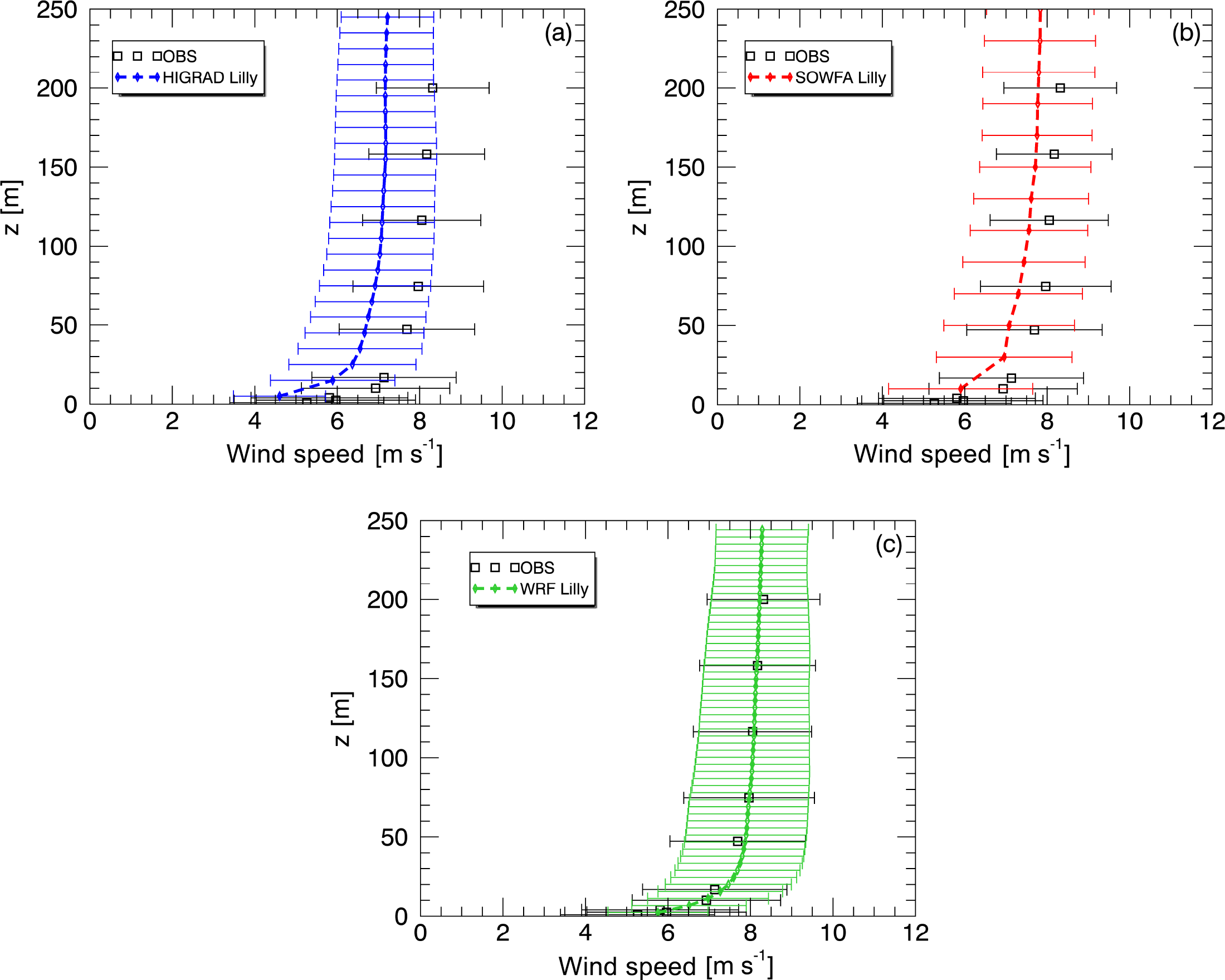
Figure 15Comparison of variability in observed and simulated wind speed profiles using all three solvers, HiGrad (a), SOWFA (b), and WRF (c), each with its optimal aspect ratio, during the convective case study.
Convective case
Simulations during convective conditions were assessed using many of the same criteria applied to the neutral simulations, again evaluated using each solver's optimal α values, here using coarser resolution than the neutral case, with HiGrad and SOWFA using grid cell sizes of 20 m in each direction, while WRF used grid spacings of 30 and 10 m, respectively. All simulations were again configured with the Lilly SFS model. HiGrad and WRF used high-order upwind schemes, with HiGrad using and WRF using O(h)=5 and O(v)=3. SOWFA used . All results presented herein are from simulations using the smaller of the two values of HS=0.35 K m s−1, corresponding to approximately 400 W m−2.
Figure 14 shows wind speed (left) and direction (right) profiles, again with “measurement variability” bars on the wind speeds indicating one standard deviation about the mean of the 10 min average values from the observations, from each solver. During convective conditions, the WRF results show the closest agreement with the mean values of the observed wind speed, with SOWFA and HiGrad producing slightly slower values. All predictions were within the range of the observed values.
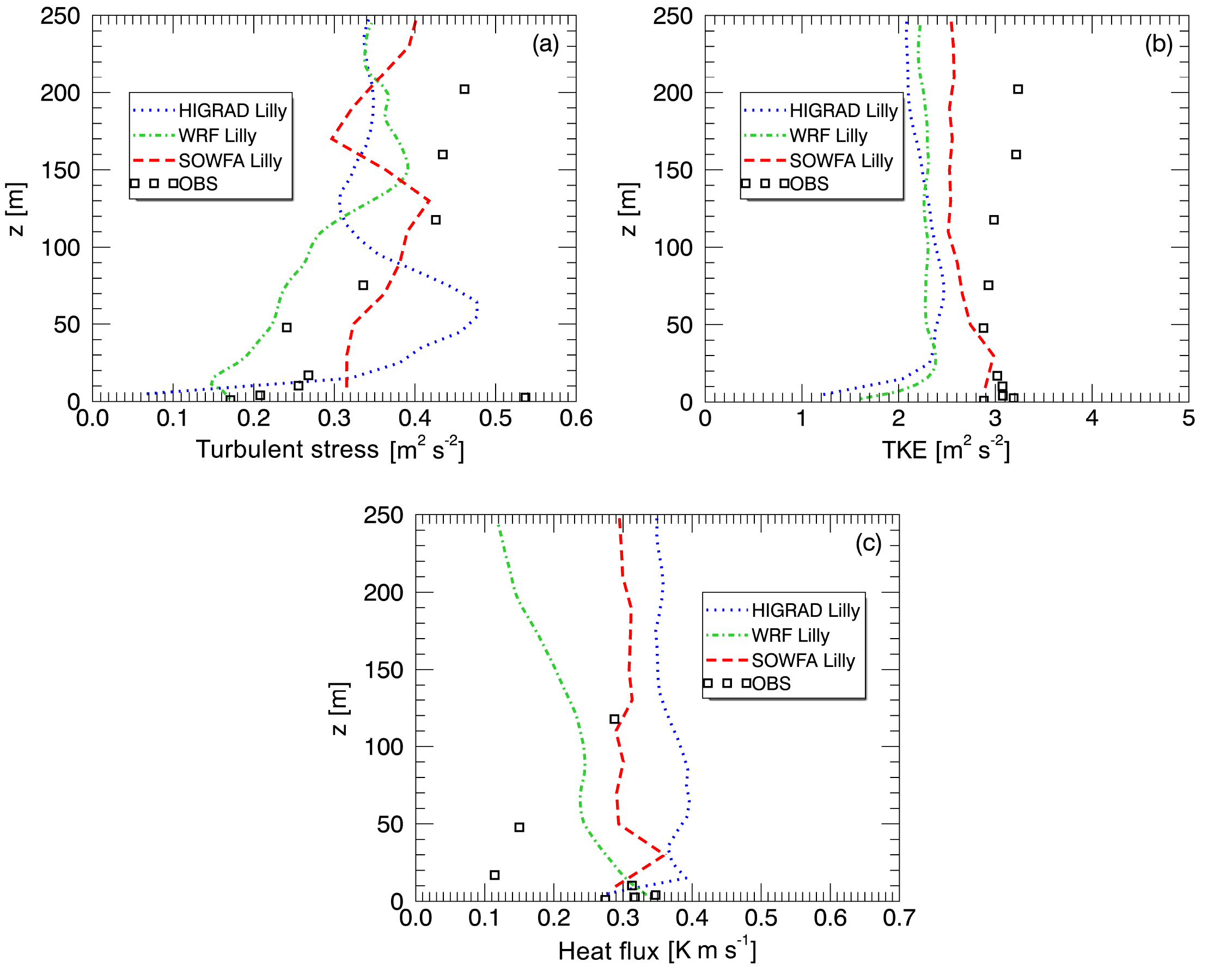
Figure 16Simulated and measured TKE (a), turbulent stress (b), and sensible heat flux (c) from the convective case study.
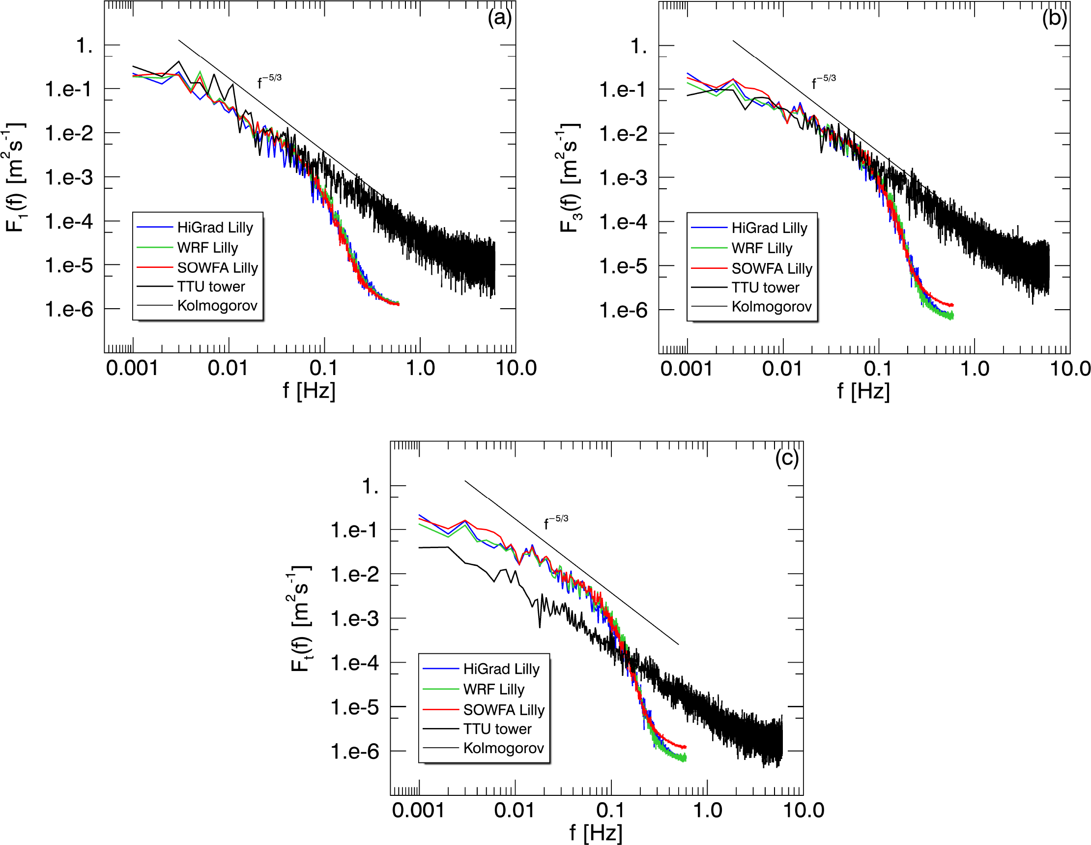
Figure 17Simulated and measured spectra of streamwise velocity (a), vertical velocity (b), and measured virtual potential temperature versus simulated vertical potential temperature (c) from the convective case study.
Figure 15 plots variability of the 10 min average wind speed values from each simulation, with the measurement variability bars signifying one standard deviation from the mean value across all 2 h of the simulation. All three models capture a similar range of wind speed variability as was observed, in contrast to the neutral case described in Sect. 3.2.1, with good agreement for the convective case attributed to the models' ability to accurately capture convective turbulent structures including updrafts and downdrafts, relatively steady geostrophic wind and surface flux forcing, and an absence of tower wake contamination given the more southerly mean wind direction.
Table 7Analysis of high-resolution LES performance using different models with the Lilly SFS parameterization for the convective ABL observed on 17 August 2012.
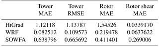
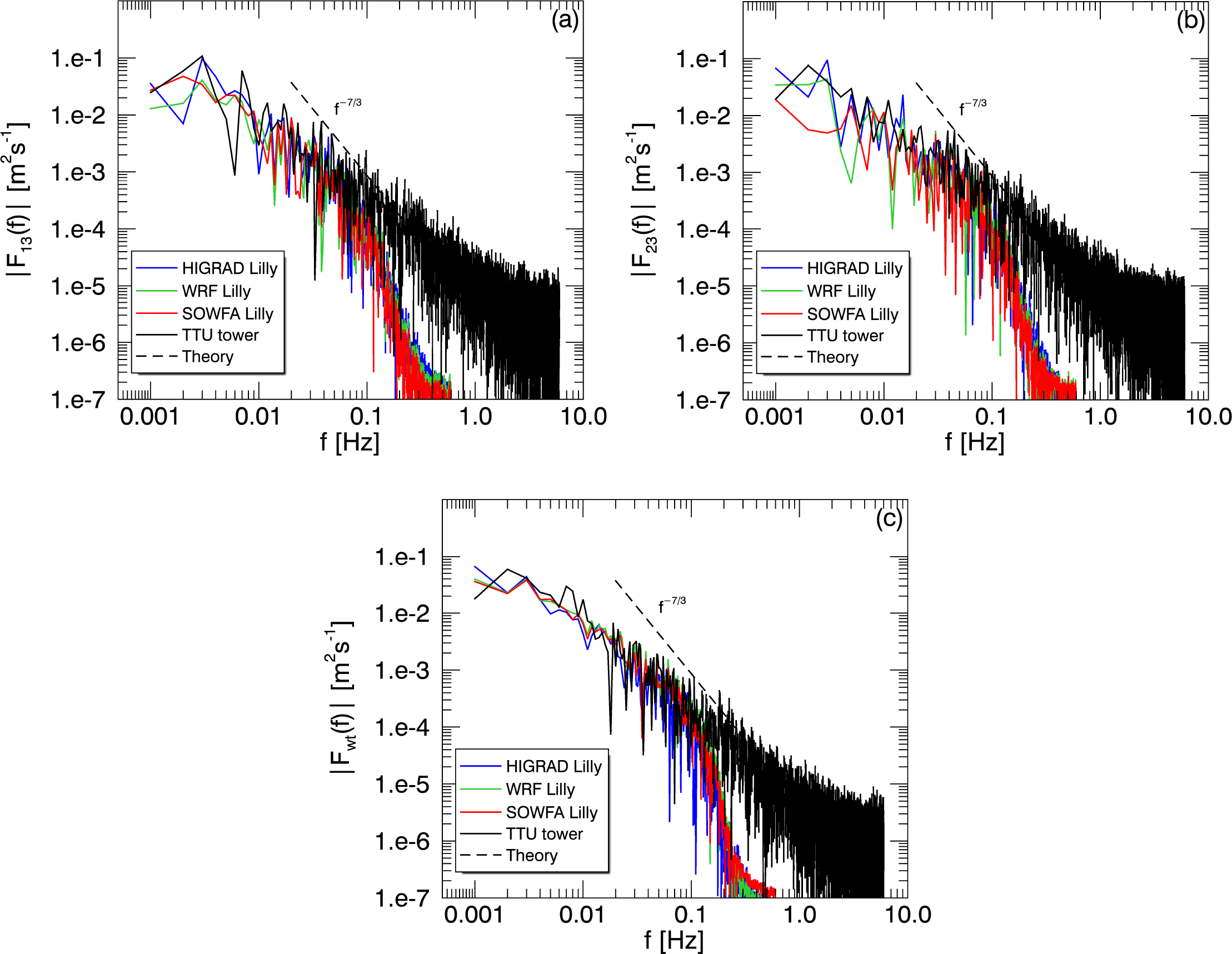
Figure 18Simulated and measured cospectra of vertical and streamwise velocity (a), vertical and spanwise velocity (b), and measured vertical velocity and virtual potential temperature versus simulated vertical velocity and potential temperature (c) from the convective case study.
Quantitative MAE and RMSE scores from the convective simulations are provided in Table 7. Computed values of MAE and RMSE across all tower levels or across the turbine rotor disk confirm our previous observation of excellent agreement between the WRF simulation results and measurements. Due to a well-mixed layer characteristic of convective ABLs, the shear over the rotor of a wind turbine is nearly zero and this is captured well by the models.
Assessment of turbulent quantities including TKE, stresses, and the sensible heat flux, was again carried out as described for the neutral conditions, here over a slightly longer 2 h period. Figure 16 shows measured versus simulated (resolved + SFS) TKE (top left), streamwise vertical stress (top right), and vertical sensible heat flux (bottom) using each solver. SOWFA provides the closest agreement of predicted TKE with the observations, with HiGrad and WRF predicting somewhat smaller values at all heights, but especially near the surface. Turbulent stress and sensible heat fluxes both show significant variability with height, with all model results agreeing broadly with the measurements. While the observed sensible heat fluxes are based upon virtual potential temperature, , with qv the water vapor mixing ratio, the simulations were dry. Hence, while exact comparison of simulated and observed heat fluxes is not possible, the dry conditions during the case study minimize discrepancies between these quantities.
Similar to the neutral case, spectra and cospectra are again computed, here by dividing 2 h time series into overlapping 20 min intervals (overlapping over 10 min) and averaging the resulting 11 spectra. Figure 17 shows observed and simulated spectra of the streamwise velocity (top left), vertical velocity (top right), as well as observed θv and simulated θ spectra (bottom). For the velocity, agreement between the simulated and observed lower-frequency spectral content is good, with the expected attenuation of higher-frequency content from the simulated spectra due to filtering effects of the grid and numerics, as described in Sect. 3.2.1.3. Spectra of temperature variables show greater low-frequency power from the simulations, possibly due to the specified value of HS being greater than the actual values (which are not available).
Figure 18 shows cospectra of the vertical velocity with the streamwise (upper left) and spanwise (upper right) components, as for the neutral case, along with those of the measured vertical velocity and θv, versus simulated vertical velocity and θ (bottom). As with the spectra, measured and simulated cospectra likewise show good agreement, including the sensible heat flux cospectrum, even though simulated temperature variance was higher than that of the observed θv (see Fig. 17c).
With a view toward assessing the utility of idealized LES to provide turbulent flow quantities of interest to wind power applications, three different LES solvers were utilized to simulate quasi-steady neutral and convective ABL flow regimes. Simulations were compared against observations over nearly flat and homogeneous surface cover, for two case studies featuring nearly steady near-neutral and convective conditions, permitting use of idealized geostrophic forcing, uniform surface conditions, and periodic LBCs. The three solvers, encompassing a range of common numerical formulations and turbulence SFS models, were subject to a series of sensitivity experiments to assess the impacts of variations of model configuration and forcing parameters on quantities of interest, including wind speed, turbulent stresses and fluxes, TKE, spectra, and cospectra.
A unique aspect of this study was computation of model turbulence statistics, spectra and cospectra, in the frequency domain, enabling direct comparison with observed values. Spectral characteristics from all simulations displayed expected qualitative characteristics, including peak energy at low wave numbers, an inertial cascade, and attenuation of power with increasing frequency. The narrower inertial subranges exhibited by the simulated versus the observed flows were due in part to lower sampling rates of the simulations, and in part to the implicit model filter imposed by the mesh and numerical discretization, the latter evidenced by the slightly wider inertial subranges from the SOWFA simulations.
Comparison with observations reveals generally good performance of all models, under a typical range of configuration and forcing variations. This supports the use of idealized LES to produce useful flow and turbulence parameters during appropriate quasi-canonical flow conditions. The convective simulations provided generally better agreement with the observations, especially in quantities expressing variability, with superior performance attributed primarily to buoyancy-generated turbulence dominating other forcing. While it is difficult to attribute the sources of discrepancies to features of the forcing versus generic limitations of the models, given the limitations of the data and simplicity of the model setups and forcing, sensitivity to different advection schemes, SFS parameterizations, and forcing was evident. An important conclusion is that the choice of advection discretization can be as important as the SFS parameterization.
Given the generally good performance of the idealized LES evaluated herein for simulating canonical, quasi-ideal cases, future efforts will focus on further identifying sources of the discrepancies between the simulations and the observations. This includes further isolation of the impacts of choices of numerical methods, domain configuration, and physical forcing parameter values on various quantities of interest. One approach will be to conduct mesoscale simulations of quasi-ideal case studies such as those examined here to obtain better estimates of various forcing parameters not available from the observations, or representable using constant values, such as changes of Ug over time, and advections of momentum and temperature. Incorporation of these additional forcing parameters may enable quasi-idealized simulations to capture a wider range of meteorological conditions, and enable further elucidation of the roles of numerical and configuration changes in simulation accuracies. Full coupling of microscale and mesoscale simulations will also be pursued, with a view toward the creation of a full-spectrum simulation capability applicable to arbitrary conditions. The present study provides a necessary first step and background support for future assessment of more general and robust mesoscale to microscale coupling techniques.
The following datasets are available at https://a2e.energy.gov/projects/mmc (last access: 25 July 2018):
-
mmc/microscale.anl.wrfles.convective.ttu (https://doi.org/10.15483/1455026, Mirocha et al., 2018a)
-
mmc/microscale.anl.wrfles.neutral.ttu (https://doi.org/10.15483/1455030, Mirocha et al., 2018b)
-
mmc/microscale.lanl.higrad.convective.ttu (https://doi.org/10.15483/1455034, Mirocha et al., 2018c)
-
mmc/microscale.lanl.higrad.neutral.ttu (https://doi.org/10.15483/1455035, Mirocha et al., 2018d)
-
mmc/microscale.lanl.wrfles.convective.ttu (https://doi.org/10.15483/1455027, Mirocha et al., 2018e)
-
mmc/microscale.lanl.wrfles.neutral.ttu (https://doi.org/10.15483/1455031, Mirocha et al., 2018f)
-
mmc/microscale.llnl.wrfles.neutral.ttu (https://doi.org/10.15483/1455029, Mirocha et al., 2018g)
-
mmc/microscale.nrel.sowfa.neutral.ttu (https://doi.org/10.15483/1455032, Mirocha et al., 2018h)
-
mmc/microscale.pnnl.wrfles.convective.ttu (https://doi.org/10.15483/1455025, Mirocha et al., 2018i)
-
mmc/mesoscale.nrel.hrrr.wfip2.d01 (https://doi.org/10.21947/1435011, Mirocha et al., 2018j)
-
mmc/mesoscale.nrel.wrf.ttutower.d03 (https://doi.org/10.21947/1435012, Mirocha et al., 2018k)
-
mmc/mesoscale.pnnl.wrf.ttutower.d03 (https://doi.org/10.21947/1435013, Mirocha et al., 2018l)
-
mmc/tower.z01.a0 (https://doi.org/10.15483/1461206,
Mirocha et al., 2018m) -
mmc/tower.z01.00 (https://doi.org/10.21947/1329252,
Mirocha et al., 2018n) -
mmc/microscale.snl.sonic.convective.ttu (https://doi.org/10.15483/1455028, Mirocha et al., 2018o)
-
mmc/radar.z01.00 (https://doi.org/10.21947/1329730,
Mirocha et al., 2018p).
The authors declare that they have no conflict of interest.
This work was performed under the auspices of the
US Department of Energy (DOE) by Lawrence Livermore National Laboratory,
the National Renewable Energy Laboratory, Los Alamos National Laboratory,
Pacific Northwest National, Argonne National Laboratory, and Sandia National
Laboratories, under contracts DE-AC52-07NA27344, DE-AC36-08GO28308,
DE-AC52-06NA25396, DE-A06-76RLO 1830, DE-AC02-06CH11357 and
DE-AC04-94AL85000, respectively. Ramesh Balakrishnan used resources of the
Argonne Leadership Computing Facility, which is a DOE Office of Science User
Facility supported under Contract DE-AC02-06CH11357. All participants were
supported by the US DOE Office of Energy Efficiency and Renewable Energy. The
US Government retains and the publisher, by accepting the article for
publication, acknowledges that the US Government retains a nonexclusive,
paid-up, irrevocable, worldwide license to publish or reproduce the published
form of this work, or allow others to do so, for US Government purposes.
Edited by: Joachim Peinke
Reviewed by: two anonymous referees
Aitken, M. L., Kosović, B., Mirocha, J. D., and Lundquist, J. K.: Large eddy simulation of wind turbine wake dynamics in the stable boundary layer using the Weather Research and Forecasting Model, J. Renew. Sustain. Ener., 6, 033137, https://doi.org/10.1063/1.4885111, 2014.
Arya, S. P.: Introduction to Micrometeorology, 2nd Edn., Academic Press, San Diego, 2001.
Bailey, B. H.: The financial impact of wind plant uncertainty, NAWEA Symposium, Boulder, CO, 26 August 2013.
Barthelmie, R. J., Folkerts, L., Ormel, T., Sanderhoff, P., Eecen, P. J., Stobbe, O., and Nielsen, N. M.: Offshore wind turbine wakes measured by sodar, J. Atmos. Ocean. Tech., 20, 466–477, https://doi.org/10.1175/1520-0426(2003)20<466:OWTWMB>2.0.CO;2, 2003.
Barthelmie, R. J., Pryor, S. C., Frandsen, S. T., Hansen, K. S., Shepers, J. G., Rados, K., Schlez, W., Neubert, A., Jensen, L. E., and Neckelmann, S: Quantifying the impact of wind turbine wakes on power output at offshore wind farms, J. Atmos. Ocean. Tech., 27, 1302–1317, https://doi.org/10.1175/2010JTECHA1398.1, 2010.
Bhaganagar, K. and Debnath, M.: Implications of stably stratified atmospheric boundary layer turbulence on the near-wake structure of wind turbines, Energies, 7, 5740–5763, https://doi.org/10.3390/en7095740, 2014.
Brasseur, J. G. and Wei, T.: Designing large-eddy simulation of the turbulent boundary layer to capture law-of-the-wall scaling, Phys. Fluids, 22, 021303, https://doi.org/10.1063/1.3319073, 2010.
Churchfield, M. J., Lee, S., Michalakes, J., and Moriarty, P. J.: A numerical study of the effects of atmospheric and wake turbulence on wind turbine dynamics, J. Turbul., 13, N14, https://doi.org/10.1080/14685248.2012.668191, 2012.
Deardorff, J. W.: A numerical study of three-dimensional turbulent channel flow at large Reynolds numbers, J. Fluid Mech., 41, 453–480, https://doi.org/10.1017/S0022112070000691, 1970.
Deardorff, J. W.: Stratocumulus-capped mixed layers derived from a three-dimensional model, Bound.-Lay. Meteorol., 18, 495–527, https://doi.org/10.1007/BF00119502, 1980.
Ercolani, G., Gorlé, C., Corbari, C., and Mancini, M.: RAMS sensitivity to grid spacing and grid aspect ratio in large-eddy simulations of the dry neutral atmospheric boundary layer, Comput. Fluids, 146, 59–73, https://doi.org/10.1016/j.compfluid.2017.01.010, 2017.
Hirth, B. M., Schroeder, J. L., Gunter, S., and J. Guynes: Measuring a Utility Scale Turbine Wake Using the TTUKa Mobile Research Radars, J. Atmos. Ocean. Tech., 29, 765–771, https://doi.org/10.1175/JTECH-D-12-00039.1, 2012.
Högström, U., Asimakopoulos, D. N., Kambezidis, H., Helmis, C. G., and Smedman, A.: A Field Study of the Wake Behind a 2 MW Wind Turbine, Atmos. Environ., 22, 803–820, https://doi.org/10.1016/0004-6981(88)90020-0, 1988.
Holton, J. R.: An Introduction to Dynamic Meteorology, 3rd Edn., Academic Press, USA, 1992.
Iungo, G., Wu, Y-T., and Porté-Agel, F.: Field measurements of wind turbine wakes with Lidars, J. Atmos. Oceanic Technol., 30, 274–287, https://doi.org/10.1175/JTECH-D-12-00051.1, 2013.
Jonkman, J. M. and Buhl Jr., M. L.: FAST Manual User's Guide, NREL report No. NREL/EL-500-38230, 2005.
Kelley, C. L. and Ennis, B. L.: SWiFT Site Atmospheric Characterization, Tech. Rep. SAND2016-0216, Sandia National Laboratories, Albuquerque, NM, 2016.
Kosović, B.: Subgrid-scale modeling for the large-eddy simulation of high-Reynolds-number boundary layers, J. Fluid Mech., 336, 151–182, https://doi.org/10.1017/S0022112096004697, 1997.
Kosović, B. and Curry, J. A.: A large eddy simulation study of a quasi-steady, stably stratified atmospheric boundary layer, J. Atmos. Sci., 57, 1052–1068, https://doi.org/10.1175/1520-0469(2000)057<1052:ALESSO>2.0.CO;2, 2000.
Kosović B., Pullin, D. I., and Samtaney, R.: Subgrid-scale modeling for large-eddy simulations of compressible turbulence, Phys. Fluids, 14, 1511–1522, https://doi.org/10.1063/1.1458006, 2002.
Lilly, D. K.: The representation of small-scale turbulence in numerical experiment, Proc. IBM Scientific Computing Symp. on Environmental Sciences, White Plains, NY, IBM, 195–210, 1967.
Lu, H. and Porté-Agel, F: Large-eddy simulation of a very large wind farm in a stable atmospheric boundary layer, Phys. Fluids, 23, 065101, https://doi.org/10.1063/1.3589857, 2011.
Lund, T., Wu, X., and Squires, K.: Generation of turbulent inflow data for spatially developing boundary-layer simulations, J. Comput. Phys., 140, 233–258, https://doi.org/10.1006/jcph.1998.5882, 1998.
Mayor, S., Spalart, P., and Tripoli, G: Application of a perturbation recycling method in the large-eddy simulation of a mesoscale convective internal boundary layer, J. Atmos. Sci., 59, 2385–2395, https://doi.org/10.1175/1520-0469(2002)059<2385:AOAPRM>2.0.CO;2, 2002.
Magnusson, M. and Smedman, A.: Influence of Atmospheric Stability on Wind Turbine Wakes, Wind Energy, 18, 139–152, 1994.
Mehta, D., van Zuijlen, A. H., Koren, B., Holierhoek, J. G., and Bijl, H.: Large Eddy Simulation of wind farm aerodynamics: A review, J. Wind Eng. Ind. Aerod., 133, 1–17, https://doi.org/10.1016/j.jweia.2014.07.002, 2014.
Mirocha, J. D., Lundquist, J. K., and Kosović, B.: Implementation of a nonlinear subfilter turbulence stress model for large-eddy simulation in the Advanced Research WRF Model, Mon. Weather Rev., 138, 4212–4228, https://doi.org/10.1175/2010MWR3286.1, 2010.
Mirocha, J. D., Kosović, B., and Kirkil, G.: Resolved turbulence characteristics in large-eddy simulations nested within mesoscale simulations using the Weather Research and Forecasting model, Mon. Weather Rev., 142, 806–831, https://doi.org/10.1175/MWR-D-13-00064.1, 2014a.
Mirocha, J. D., Kosović, B., Aitken, M. L., and Lundquist, J. K.: Implementation of a generalized actuator disk wind turbine model into the weather research and forecasting model for large-eddy simulation applications, J. Renew. Sustain. Ener., 6, 013104, https://doi.org/10.1063/1.4861061, 2014b.
Mirocha, J. D., Churchfield, M. J., Munoz-Esparza, D., Rai, R. K., Feng, Y., Kosovic, B., Haupt, S. E., Brown, B., Ennis, B. L., Draxl, C., Sanz Rodrigo, J., Shaw, W. J., Berg, L. K., Moriarty, P. J., Linn, R. R., Kotamarthi, R. V., Balakrishnan, R., Cline, J. W., Robinson, M. C., and Ananthan, S.: mmc/microscale.anl.wrfles.convective.ttu, Atmosphere to Electrons (A2e), https://doi.org/10.15483/1455026, 2018a.
Mirocha, J. D., Churchfield, M. J., Munoz-Esparza, D., Rai, R. K., Feng, Y., Kosovic, B., Haupt, S. E., Brown, B., Ennis, B. L., Draxl, C., Sanz Rodrigo, J., Shaw, W. J., Berg, L. K., Moriarty, P. J., Linn, R. R., Kotamarthi, R. V., Balakrishnan, R., Cline, J. W., Robinson, M. C., and Ananthan, S.: mmc/microscale.anl.wrfles.neutral.ttu, Atmosphere to Electrons (A2e), https://doi.org/10.15483/1455026, 2018b.
Mirocha, J. D., Churchfield, M. J., Munoz-Esparza, D., Rai, R. K., Feng, Y., Kosovic, B., Haupt, S. E., Brown, B., Ennis, B. L., Draxl, C., Sanz Rodrigo, J., Shaw, W. J., Berg, L. K., Moriarty, P. J., Linn, R. R., Kotamarthi, R. V., Balakrishnan, R., Cline, J. W., Robinson, M. C., and Ananthan, S.: mmc/microscale.lanl.higrad.convective.ttu, Atmosphere to Electrons (A2e), https://doi.org/10.15483/1455034, 2018c.
Mirocha, J. D., Churchfield, M. J., Munoz-Esparza, D., Rai, R. K., Feng, Y., Kosovic, B., Haupt, S. E., Brown, B., Ennis, B. L., Draxl, C., Sanz Rodrigo, J., Shaw, W. J., Berg, L. K., Moriarty, P. J., Linn, R. R., Kotamarthi, R. V., Balakrishnan, R., Cline, J. W., Robinson, M. C., and Ananthan, S.: mmc/microscale.lanl.higrad.neutral.ttu, Atmosphere to Electrons (A2e), https://doi.org/10.15483/1455035, 2018d.
Mirocha, J. D., Churchfield, M. J., Munoz-Esparza, D., Rai, R. K., Feng, Y., Kosovic, B., Haupt, S. E., Brown, B., Ennis, B. L., Draxl, C., Sanz Rodrigo, J., Shaw, W. J., Berg, L. K., Moriarty, P. J., Linn, R. R., Kotamarthi, R. V., Balakrishnan, R., Cline, J. W., Robinson, M. C., and Ananthan, S.: mmc/microscale.lanl.wrfles.convective.ttu, Atmosphere to Electrons (A2e), https://doi.org/10.15483/1455027, 2018e.
Mirocha, J. D., Churchfield, M. J., Munoz-Esparza, D., Rai, R. K., Feng, Y., Kosovic, B., Haupt, S. E., Brown, B., Ennis, B. L., Draxl, C., Sanz Rodrigo, J., Shaw, W. J., Berg, L. K., Moriarty, P. J., Linn, R. R., Kotamarthi, R. V., Balakrishnan, R., Cline, J. W., Robinson, M. C., and Ananthan, S.: mmc/microscale.lanl.wrfles.neutral.ttu, Atmosphere to Electrons (A2e), https://doi.org/10.15483/1455031, 2018f.
Mirocha, J. D., Churchfield, M. J., Munoz-Esparza, D., Rai, R. K., Feng, Y., Kosovic, B., Haupt, S. E., Brown, B., Ennis, B. L., Draxl, C., Sanz Rodrigo, J., Shaw, W. J., Berg, L. K., Moriarty, P. J., Linn, R. R., Kotamarthi, R. V., Balakrishnan, R., Cline, J. W., Robinson, M. C., and Ananthan, S.: mmc/microscale.llnl.wrfles.neutral.ttu, Atmosphere to Electrons (A2e), https://doi.org/10.15483/1455029, 2018g.
Mirocha, J. D., Churchfield, M. J., Munoz-Esparza, D., Rai, R. K., Feng, Y., Kosovic, B., Haupt, S. E., Brown, B., Ennis, B. L., Draxl, C., Sanz Rodrigo, J., Shaw, W. J., Berg, L. K., Moriarty, P. J., Linn, R. R., Kotamarthi, R. V., Balakrishnan, R., Cline, J. W., Robinson, M. C., and Ananthan, S.: mmc/microscale.nrel.sowfa.neutral.ttu, Atmosphere to Electrons (A2e), https://doi.org/10.15483/1455032, 2018h.
Mirocha, J. D., Churchfield, M. J., Munoz-Esparza, D., Rai, R. K., Feng, Y., Kosovic, B., Haupt, S. E., Brown, B., Ennis, B. L., Draxl, C., Sanz Rodrigo, J., Shaw, W. J., Berg, L. K., Moriarty, P. J., Linn, R. R., Kotamarthi, R. V., Balakrishnan, R., Cline, J. W., Robinson, M. C., and Ananthan, S.: mmc/microscale.pnnl.wrfles.convective.ttu, Atmosphere to Electrons (A2e), https://doi.org/10.15483/1455025, 2018i.
Mirocha, J. D., Churchfield, M. J., Munoz-Esparza, D., Rai, R. K., Feng, Y., Kosovic, B., Haupt, S. E., Brown, B., Ennis, B. L., Draxl, C., Sanz Rodrigo, J., Shaw, W. J., Berg, L. K., Moriarty, P. J., Linn, R. R., Kotamarthi, R. V., Balakrishnan, R., Cline, J. W., Robinson, M. C., and Ananthan, S.: mmc/mesoscale.nrel.hrrr.wfip2.d01, Atmosphere to Electrons (A2e), https://doi.org/10.21947/1435011, 2018j.
Mirocha, J. D., Churchfield, M. J., Munoz-Esparza, D., Rai, R. K., Feng, Y., Kosovic, B., Haupt, S. E., Brown, B., Ennis, B. L., Draxl, C., Sanz Rodrigo, J., Shaw, W. J., Berg, L. K., Moriarty, P. J., Linn, R. R., Kotamarthi, R. V., Balakrishnan, R., Cline, J. W., Robinson, M. C., and Ananthan, S.: mmc/mesoscale.nrel.wrf.ttutower.d03, Atmosphere to Electrons (A2e), https://doi.org/10.21947/1435012, 2012k.
Mirocha, J. D., Churchfield, M. J., Munoz-Esparza, D., Rai, R. K., Feng, Y., Kosovic, B., Haupt, S. E., Brown, B., Ennis, B. L., Draxl, C., Sanz Rodrigo, J., Shaw, W. J., Berg, L. K., Moriarty, P. J., Linn, R. R., Kotamarthi, R. V., Balakrishnan, R., Cline, J. W., Robinson, M. C., and Ananthan, S.: mmc/mesoscale.pnnl.wrf.ttutower.d03, Atmosphere to Electrons (A2e), https://doi.org/10.21947/1435013, 2012l.
Mirocha, J. D., Churchfield, M. J., Munoz-Esparza, D., Rai, R. K., Feng, Y., Kosovic, B., Haupt, S. E., Brown, B., Ennis, B. L., Draxl, C., Sanz Rodrigo, J., Shaw, W. J., Berg, L. K., Moriarty, P. J., Linn, R. R., Kotamarthi, R. V., Balakrishnan, R., Cline, J. W., Robinson, M. C., and Ananthan, S.: mmc/tower.z01.a0, Atmosphere to Electrons (A2e), https://doi.org/10.15483/1461206, 2012m.
Mirocha, J. D., Churchfield, M. J., Munoz-Esparza, D., Rai, R. K., Feng, Y., Kosovic, B., Haupt, S. E., Brown, B., Ennis, B. L., Draxl, C., Sanz Rodrigo, J., Shaw, W. J., Berg, L. K., Moriarty, P. J., Linn, R. R., Kotamarthi, R. V., Balakrishnan, R., Cline, J. W., Robinson, M. C., and Ananthan, S.: mmc/tower.z01.00, Atmosphere to Electrons (A2e), https://doi.org/10.21947/1329252, 2018n.
Mirocha, J. D., Churchfield, M. J., Munoz-Esparza, D., Rai, R. K., Feng, Y., Kosovic, B., Haupt, S. E., Brown, B., Ennis, B. L., Draxl, C., Sanz Rodrigo, J., Shaw, W. J., Berg, L. K., Moriarty, P. J., Linn, R. R., Kotamarthi, R. V., Balakrishnan, R., Cline, J. W., Robinson, M. C., and Ananthan, S.: mmc/microscale.snl.sonic.convective.ttu, Atmosphere to Electrons (A2e), https://doi.org/10.15483/1455028, 2012o.
Mirocha, J. D., Churchfield, M. J., Munoz-Esparza, D., Rai, R. K., Feng, Y., Kosovic, B., Haupt, S. E., Brown, B., Ennis, B. L., Draxl, C., Sanz Rodrigo, J., Shaw, W. J., Berg, L. K., Moriarty, P. J., Linn, R. R., Kotamarthi, R. V., Balakrishnan, R., Cline, J. W., Robinson, M. C., and Ananthan, S.: mmc/radar.z01.00, Atmosphere to Electrons (A2e), https://doi.org/10.21947/1329730, 2018p.
Moeng, C.-H.: A Large-Eddy-Simulation Model for the Study of Planetary Boundary-Layer Turbulence, J. Atmos. Sci., 41, 2052–2062, https://doi.org/10.1175/1520-0469(1984)041<2052:ALESMF>2.0.CO;2, 1984.
Monin, A. S. and Obukhov, A. M.: Basic laws of turbulent mixing in the surface layer of the atmosphere, Tr.-Akad. Nauk SSSR Geofiz. Inst., 24, 163–187, 1954.
Muñoz-Esparza, D., Kosović, B., Mirocha, J. D., and van Beek, J.: Bridging the transition from mesoscales to microscale turbulence in atmospheric models, Bound.-Lay. Meteorol., 153, 409–440, https://doi.org/10.1007/s10546-014-9956-9, 2014.
Muñoz-Esparza, D., Kosović, B., van Beek, D., and Mirocha, J. D.: A stochastic perturbation method to generate inflow turbulence in large-eddy simulation models: application to neutrally stratified atmospheric boundary layers, Phys. Fluids, 27, 035102, https://doi.org/10.1063/1.4913572, 2015.
Muñoz-Esparza, D., Lundquist, J. K., Sauer, J. A., Kosović, B., and Linn, R. R.: Coupled mesoscale-LES modeling of a diurnal cycle during the CWEX-13 field campaign: From weather to boundary-layer eddies, J. Adv. Model. Earth Sy., 9, 1572–1594, https://doi.org/10.1002/2017MS000960, 2017.
Nygaard, N. G.: Lidar wake measurements in an onshore wind farm, VindKraftNet: Remote Sensing Workshop, Roskilde, Denmark, 2011.
OpenFOAM: The Open Source CFD Toolbox, created by OpenCFD Ltd (ESI Group), distributed online at: http://www.openfoam.com, last access: 15 August 2018.
Rai, R. K., Berg, L. K., Kosović, B., Mirocha, J. D., Pekour, M. S., and Shaw, W. J.: Comparison of Measured and Numerically Simulated Turbulence Statistics in a Convective Boundary Layer Over Complex Terrain, Bound.-Lay. Meteorol., 163, 69–89, https://doi.org/10.1007/s10546-016-0217-y, 2017a.
Rai, R. K., Berg, L. K., Pekour, M., Shaw, W. J., Kosović, B., Mirocha, J. D., and Ennis, B. L.: Spatiotemporal Variability of Turbulence Kinetic Energy Budgets in the Convective Boundary Layer over Both Simple and Complex Terrain, J. Appl. Meteorol. Clim., 56, 3285–3302, https://doi.org/10.1175/JAMC-D-17-0124.1, 2017b.
Rhodes, M. E. and Lundquist, J. K.: The effect of wind-turbine wakes on summertime US Mid-west atmospheric wind profiles as observed with ground-based Doppler lidar, Bound.-Lay. Meteorol., 149, 85–103, https://doi.org/10.1007/s10546-013-9834-x, 2013.
Sanderse, B., van der Pijl, S. P., and Koren, B.: Review of computational fluid dynamics for wind turbine wake aerodynamics, Wind Energy, 14, 799–819, https://doi.org/10.1002/we.458, 2011.
Sanz Rodrigo, J., Churchfield, M., and Kosovic, B.: A methodology for the design and testing of atmospheric boundary layer models for wind energy applications, Wind Energ. Sci., 2, 35–54, https://doi.org/10.5194/wes-2-35-2017, 2017.
Sauer, J. A., Muñoz-Esparza, D., Canfield, J. M., Costigan, K. R., Linn, R. R., and Kim, Y. J.: A Large-Eddy Simulation Study of Atmospheric Boundary Layer Influence on Stratified Flows over Terrain, J. Atmos. Sci., 73, 2615–2632, https://doi.org/10.1175/JAS-D-15-0282.1, 2016.
Shaw, W. J., Lundquist, J. K., and Schreck, S. J.: Workshop on Research Needs for Wind Resource Characterization, B. Am. Meteorol. Soc., 90, 535538, https://doi.org/10.1175/2008BAMS2729.1, 2009.
Sim, C., Basu, S., and Manuel, L.: The influence of stable boundary layer flows on wind turbine fatigue loads, in: Proceedings of the AIAA aerospace sciences meeting, Orlando, FL, 2009.
Skamarock, W. C.: Evaluating mesoscale NWP models using kinetic energy spectra, Mon. Weather Rev., 132, 3019–3032, https://doi.org/10.1175/MWR2830.1, 2004.
Skamarock, W. C., Klemp, J. B., Dudhia, J., Gill, D. O., Barker, D. M., Duda, M. G., Huang, X.-Y., Wang, W., and Powers, J. G.: A description of the advanced research WRF version 3, Report No. NCAR/TN-4751STR, National Center for Atmospheric Research, Boulder, CO, 2008.
Smagorinsky, J.: General circulation experiments with the primitive equations, Mon. Weather Rev., 91, 99–152, https://doi.org/10.1175/1520-0493(1963)091<0099:GCEWTP>2.3.CO;2, 1963.
Smalikho, I. N., Banakh, V. A., Pichugina, Y. L., Brewer, W. A., Banta, R. M., Lundquist, J. K., and Kelley, N. D.: Lidar investigation of atmosphere effect on a wind turbine wake, J. Atmos. Ocean. Tech., 30, 2554–2570, https://doi.org/10.1175/JTECH-D-12-00108.1, 2013.
Sullivan, P. P., McWilliams, J. C., and Moeng, C.-H.: A subgrid-scale model for large-eddy simulation of planetary boundary-layer flows, Bound.-Lay. Meteorol., 71, 247–276, https://doi.org/10.1007/BF00713741, 1994.
Stull, R. B.: An Introduction to Boundary Layer Meteorology, Kluwer Academic Publisher, Netherlands, 1988.
Troldborg, N., Larsen, G. C., Madsen, H. A., Hansen, K. S., Sørensen, J. N., and Mikkelsen, R.: Numerical simulations of wake interaction between two wind turbines at various inflow conditions, Wind Energy, 14, 859–876, https://doi.org/10.1002/we.433, 2011.
Veers, P. S.: Three-Dimensional Wind Simulation, SAND88-0152, Sandia National Laboratories, Albuquerque, NM, 1988.
Xie, Z. T. and Castro, I. P.: Efficient generation of inflow conditions for large eddy simulations of street-scale flows, Flow Turbul. Combust., 81, 449–470, https://doi.org/10.1007/s10494-008-9151-5, 2008.