the Creative Commons Attribution 4.0 License.
the Creative Commons Attribution 4.0 License.
 | 16 Oct 2018
An efficient frequency-domain model for quick load analysis of floating offshore wind turbines
Michael Borg
Henrik Bredmose
A model for Quick Load Analysis of Floating wind turbines (QuLAF) is presented and validated here. The model is a linear, frequency-domain, efficient tool with four planar degrees of freedom: floater surge, heave, pitch and first tower modal deflection. The model relies on state-of-the-art tools from which hydrodynamic, aerodynamic and mooring loads are extracted and cascaded into QuLAF. Hydrodynamic and aerodynamic loads are pre-computed in WAMIT and FAST, respectively, while the mooring system is linearized around the equilibrium position for each wind speed using MoorDyn. An approximate approach to viscous hydrodynamic damping is developed, and the aerodynamic damping is extracted from decay tests specific for each degree of freedom. Without any calibration, the model predicts the motions of the system in stochastic wind and waves with good accuracy when compared to FAST. The damage-equivalent bending moment at the tower base is estimated with errors between 0.2 % and 11.3 % for all the load cases considered. The largest errors are associated with the most severe wave climates for wave-only conditions and with turbine operation around rated wind speed for combined wind and waves. The computational speed of the model is between 1300 and 2700 times faster than real time.
- Article
(5161 KB) - Full-text XML
- BibTeX
- EndNote


Offshore wind energy is a key contributor to a carbon-free energy supply. Most of today's offshore wind farms are bottom-fixed, meaning their feasibility is limited to shallow and intermediate water depths. On the other hand, the wind resource in deep water represents an enormous potential that can be unlocked with the deployment of floating wind farms. An important step in making floating wind turbines economically feasible is the application of larger wind turbines and the ability to design the floater to a minimum cost. The design of a floating substructure for offshore wind deployment depends on many design variables, and each possible combination is a potential design. In the design process, the candidate designs need to be simulated in different environmental conditions in order to assess the magnitude of the motions and loads in the system. These simulations are typically carried out with time-domain numerical tools, which allow a representative modelling of the physical phenomena involved and can simulate at about real-time CPU speed. However, this approach can be computationally expensive, especially if one needs to evaluate different floater designs under several environmental conditions. For an improved design process, faster tools are needed to allow optimization in the initial design stage, where the design space has to be thoroughly explored and a broad overview of the system response is desirable.
A few studies of simplified design models for offshore wind turbine floaters exist in the literature. Lupton (2014) presented a frequency-domain numerical tool for the analysis of the OC3-Hywind spar floating wind turbine (Jonkman, 2010), with eight degrees of freedom (DoFs): one normal mode per blade, two tower fore-aft modes, and floater surge, heave and pitch. The model included linear hydrodynamics computed with a potential-flow panel code. The aerodynamic forces were included through harmonic linearization, and the mooring lines were represented by a stiffness matrix. The frequency-domain code was benchmarked against an equivalent Bladed (DNV-GL AS, 2016) model with Morison-based hydrodynamics, and with a stiffness mooring matrix. Neither the frequency-domain model nor the Bladed model included viscous drag. Results were shown for regular waves and uniform, harmonic wind, and the frequency-domain code was reported to be up to 37 times faster than the Bladed model. In Lemmer et al. (2016), simplified time-domain models of the OC3-Hywind spar (Jonkman, 2010) and OC4-DeepCwind semi-submersible (Robertson et al., 2014) floating wind turbines were introduced. The models had four DoFs: floater surge and pitch, tower first fore-aft mode, and rotor azimuthal position. Linear hydrodynamics from a radiation-diffraction panel code were included in the time-domain model through the Cummins equation (Cummins, 1962). Aerodynamics were computed by coupling the code to AeroDyn. Quasi-static mooring forces were computed by solving the catenary mooring equations at each time step. A linearized version of the code was also presented. In the results, the linearized frequency-domain version was successfully benchmarked against the nonlinear time-domain version, by comparing the linear transfer function from wave height to tower-top displacement with its nonlinear equivalent. The work of Wang et al. (2017) involved a frequency-domain model of the DeepCwind semi-submersible (Robertson et al., 2014) with two rigid-body DoFs: floater surge and pitch. Linear hydrodynamics, linearized drag and drift forces were computed with the commercial software AQWA. The aerodynamic loads were included through a linearized version of the actuator point equation, where the aerodynamic contribution was divided into a constant force and a damping term – thus neglecting stochastic wind forcing. The mooring loads were included through a stiffness matrix, obtained from both quasi-static and dynamic mooring models. The model was validated against DeepCwind test data in terms of natural frequencies, response-amplitude operators and power spectral density (PSD) plots of surge and pitch response, generally obtaining a good agreement. However, a frequency-domain model for floating wind turbines able to incorporate realistic aerodynamic loads is still needed.
For bottom-fixed offshore wind turbines, Schløer et al. (2018) recently developed an efficient, frequency-domain model named QuLA (Quick Load Analysis), considering the DTU 10 MW Reference Wind Turbine (RWT; Bak et al., 2013). The mono-pile foundation and the wind turbine tower were defined as an Euler beam, and the first fore-aft modal deflection of this beam was the only DoF. Inspired by the work of van der Tempel (2006), the rotor and nacelle were represented by a point mass at the tower top, and aerodynamic loads and damping coefficients were pre-computed in the time-domain aero-elastic tool Flex5 (Øye, 1996). Compared to the work of van der Tempel (2006), the aerodynamic damping in QuLA was considered as dependent on mean wind speed. Hydrodynamic forcing was included through the Morison equation (Morison et al., 1950), where the structure velocity and acceleration were neglected. The code was validated against Flex5 in terms of time series, PSD, exceedance probability curves and fatigue damage-equivalent load (DEL). The bending moment at the seabed was estimated by QuLA within a 5 % error, and the code was reported to be approximately 40 times faster than its Flex5 equivalent.
This study presents the extension of QuLA to floating offshore wind turbines. The resulting model, QuLAF (Quick Load Analysis of Floating wind turbines), was first presented in Pegalajar-Jurado et al. (2016), with only two DoFs: floater surge and tower first fore-aft bending mode. Here we present an improved version of the model, a frequency-domain code that captures the four dominant DoFs in the in-plane global motion: floater surge, heave and pitch, and tower first fore-aft modal deflection. The model, which is here adapted to the DTU 10 MW RWT mounted on the OO-Star Wind Floater Semi 10 MW (Yu et al., 2018) was set up through cascading techniques. In the cascading process, information is pre-computed or extracted from more advanced models (parent models) to enhance the simplified models (children models). In this case, the hydrodynamic loads are extracted from the radiation-diffraction potential-flow solver WAMIT (Lee and Newman, 2016). The aerodynamic loads and aerodynamic damping coefficients are pre-computed in the numerical tool FAST v8 (Jonkman and Jonkman, 2016), and the mooring module MoorDyn (Hall, 2017) is employed to extract a mooring stiffness matrix for different operating positions. This way, the model includes standard radiation-diffraction theory and realistic rotor loads through pre-computed aero-elastic simulations. In the model, the system response is obtained by solving the linear equations of motion (EoMs) in the frequency domain, leading to a very efficient tool. While the radiation-diffraction results allow for a full linear response evaluation for rigid structure motion in waves, the ambition of this model is to extend them with the flexible tower and realistic stochastic rotor loads, thus going one step further than other simplified models in the literature. The results from QuLAF are here benchmarked against results from its time-domain, state-of-the-art (SoA) parent model in terms of time series, PSD, exceedance probability and fatigue DEL. We assess the strengths and weaknesses of the cascading process by comparison with the original time-domain model, and further develop techniques to improve the accuracy of the simplified model with respect to planar motion and tower-base loads. In this way, the potential of the model as a reliable tool for pre-design and as a complement to SoA models is demonstrated. The idea is that once the conceptual floater design is established with the efficient pre-design model, more advanced SoA models can be used for further design verification with a full design load basis that includes extreme and transient events.

Figure 1The OO-Star Wind Floater Semi 10 MW concept (http://www.olavolsen.no; last access: 24 November 2017).
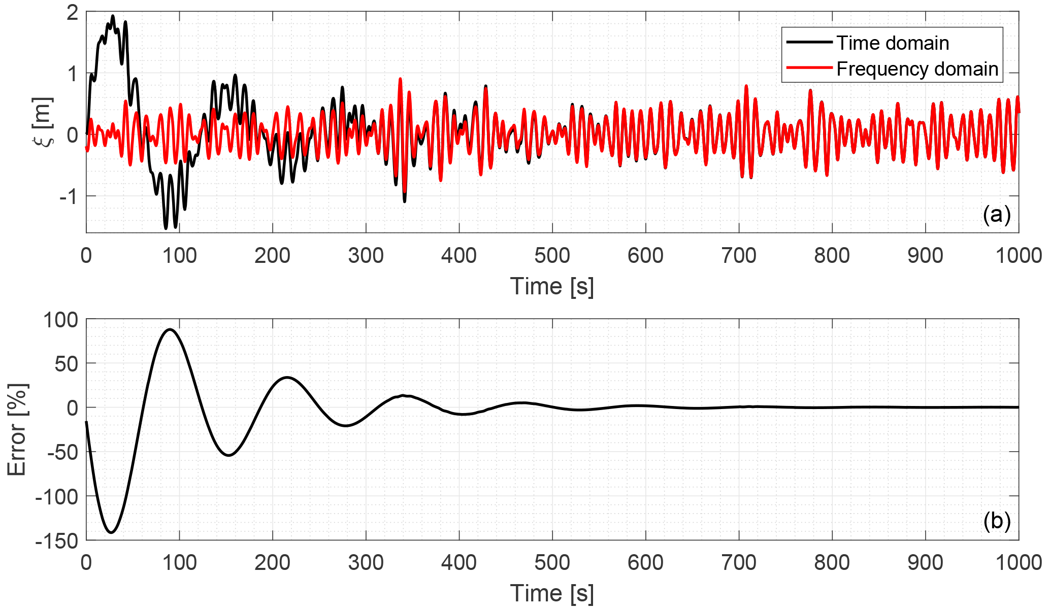
Figure 2(a) Surge response of the OC3-Hywind floating wind turbine (Jonkman, 2010) to stochastic hydrodynamic linear forcing in a one-DoF linear model, computed in both the time and frequency domains. (b) Relative error between the time- and frequency-domain solutions. Only the first 1000 s are shown.
The floating wind turbine chosen for the present study is the DTU 10 MW RWT (Bak et al., 2013) mounted on the OO-Star Wind Floater Semi 10 MW (Yu et al., 2018). The main properties of the DTU 10 MW RWT are given in Table 1, and further information can be found in Bak et al. (2013). The basic DTU Wind Energy controller (Hansen and Henriksen, 2013) is utilized, and tuned to avoid the floater pitch instability (commonly known as the “negative damping problem”) reported in, for example, Larsen and Hanson (2007).
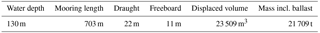
The floating substructure (see Fig. 1), developed by Dr.techn. Olav Olsen AS (http://www.olavolsen.no; last access: 24 November 2017), is a semi-submersible floater made of post-tensioned concrete. It has a central column and three outer columns mounted on a star-shaped pontoon with three legs. Each outer column is connected to the seabed by a catenary mooring line with a suspended clump weight. The main properties of the floating substructure are collected in Table 2, and further information can be found in Yu et al. (2018).
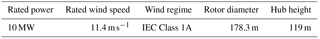
Table 2Key figures for the OO-Star Wind Floater Semi 10 MW anchored at the selected site.
Floating wind turbines can be considered harmonic oscillators with multiple coupled DoFs. To illustrate the strengths and weaknesses of solving the relevant EoM in the time or the frequency domain, a simple one-DoF mass-spring-damper system is considered,
where m is the system mass, b is the damping coefficient, c is the restoring coefficient, ξ(t) is the system displacement from its equilibrium position, and F(t) is a harmonic excitation force. Equation (1) can be also written in complex notation, by expressing the excitation force at the frequency ω as , where ℜ indicates the real part, is the Fourier transform of F(t) and i is the imaginary unit. If the initial transient part of the response is neglected, the steady-state system response at the given frequency can also be written as , leading to the EoM in the frequency domain,
The frequency-domain response may be obtained by simply multiplying the frequency-domain excitation force by the transfer function H(ω). This can be done at all frequencies and, due to the linearity, one can add the results at each frequency to obtain the total solution. Thus, once has been determined for all frequencies, the time-domain response ξ(t) is obtained through an inverse Fourier transform of . If fast Fourier transform (FFT) and inverse fast Fourier transform (iFFT) are used, the solution can be obtained very quickly.
Figure 2 shows the surge response ξ(t) of a one-DoF model of the OC3-Hywind spar floating wind turbine (Jonkman, 2010) subjected to stochastic hydrodynamic linear forcing. The response labelled as “Time domain” was obtained by time-stepping of Eq. (1) with the classical fourth-order Runge–Kutta method and initial conditions ξ(0)=0 and . The response labelled as “Frequency domain” was computed by first obtaining the frequency-domain excitation force , calculating the frequency-domain response using Eq. (2) and finally going back to the time-domain response . The simulation time step was 0.025 s and the total simulated time was 5400 s, although only the first 1000 s are shown here. The time-domain solution took 69.41 s to run, while the frequency-domain solution was done in 0.03 s, or 2344 times faster. The two responses diverge at the beginning, where the time-domain solution is dominated by the transient response to the initial conditions, which is not present in the frequency-domain solution. However, after approximately 800 s (or six natural periods) and until the end of the simulation, the two solutions are practically identical, with errors between 0.2 % and 0.5 %, likely due to the time and frequency discretizations.
In addition to the gain in CPU speed, solving the EoM in the frequency domain allows for an easier handling of frequency-dependent properties, such as hydrodynamic added mass and radiation damping. On the other hand, it has also been shown that transient response due to initial conditions is only captured by time-domain models. However, as in the above example, the transient response due to initial conditions is an artifact of the time-domain formulation and is often discarded in the analysis. Perhaps the most clear disadvantage of frequency-domain models is that they can only accommodate loads that depend linearly on the response and its time derivatives, such as hydrodynamic added mass loads or hydrostatic loads. They cannot directly accommodate loads that depend on the response in a nonlinear manner, such as viscous drag from relative structural motion or catenary mooring loads. In those cases, simplified or linearized formulations have to be implemented instead.
In SoA models the nacelle, hub and floater are often considered rigid, whereas the tower and blades are flexible. The floater motion typically has six DoFs: surge, sway, heave, roll, pitch and yaw. Aerodynamics are normally computed using unsteady blade element momentum theory (Hansen, 2008). Hydrodynamics are typically represented by radiation-diffraction theory (Newman, 1980), the Morison equation or a combination of both. The mooring lines can be modelled with either quasi-static or dynamic approaches. In general, SoA models are more accurate than simplified models, but they also have a higher CPU cost.
A SoA, time-domain numerical model of the OO-Star Semi + DTU 10 MW floating wind turbine was used in this study as a parent model to QuLAF. The SoA model was implemented in FAST v8.16.00a-bjj (Jonkman and Jonkman, 2016) with active control and 15 DoFs for turbine and floater: first and second flap-wise blade modal deflections; first edge-wise blade modal deflection; drivetrain rotational flexibility; drivetrain speed; first and second fore-aft and side-side tower modal deflections; and floater surge, sway, heave, roll, pitch and yaw. The turbulent wind fields were computed in TurbSim, and the aerodynamic loads were modelled with AeroDyn v14. The basic DTU Wind Energy controller was applied through a dynamic-link library (DLL). The mooring loads, calculated by MoorDyn (Hall, 2017), included buoyancy, mass inertia and hydrodynamic loads resulting from the motion of the mooring lines in calm water. Hydrodynamic loads on the floater were first computed in WAMIT (Lee and Newman, 2016) and coupled to FAST through the Cummins equation. Viscous effects were modelled internally by the Morison drag term. Further details on the modelling of floating wind turbines in FAST can be found in Jonkman (2009), while a thorough description of the FAST model used in this study is presented in Pegalajar-Jurado et al. (2018b) and Pegalajar-Jurado et al. (2018a).
The simplest model for the dynamic analysis of floating wind turbines would only have a few DoFs, typically rigid-body motion of the floater in surge and pitch. Aerodynamic loads would be represented by a point force at the rotor hub and defined by an actuator point model. If the floating substructure is slender compared to the incident waves, a strip-theory approach may be applied to compute the hydrodynamic loads from the Morison equation. The forces exerted by the mooring system can be included through a stiffness matrix in the linear EoMs. Simplified, low-order models are very CPU efficient but their accuracy is often limited. In the following we present a simplified model that combines elements extracted from a SoA model into a very efficient tool, which aims at getting close to the accuracy of the SoA model while still retaining the CPU efficiency of low-order models.
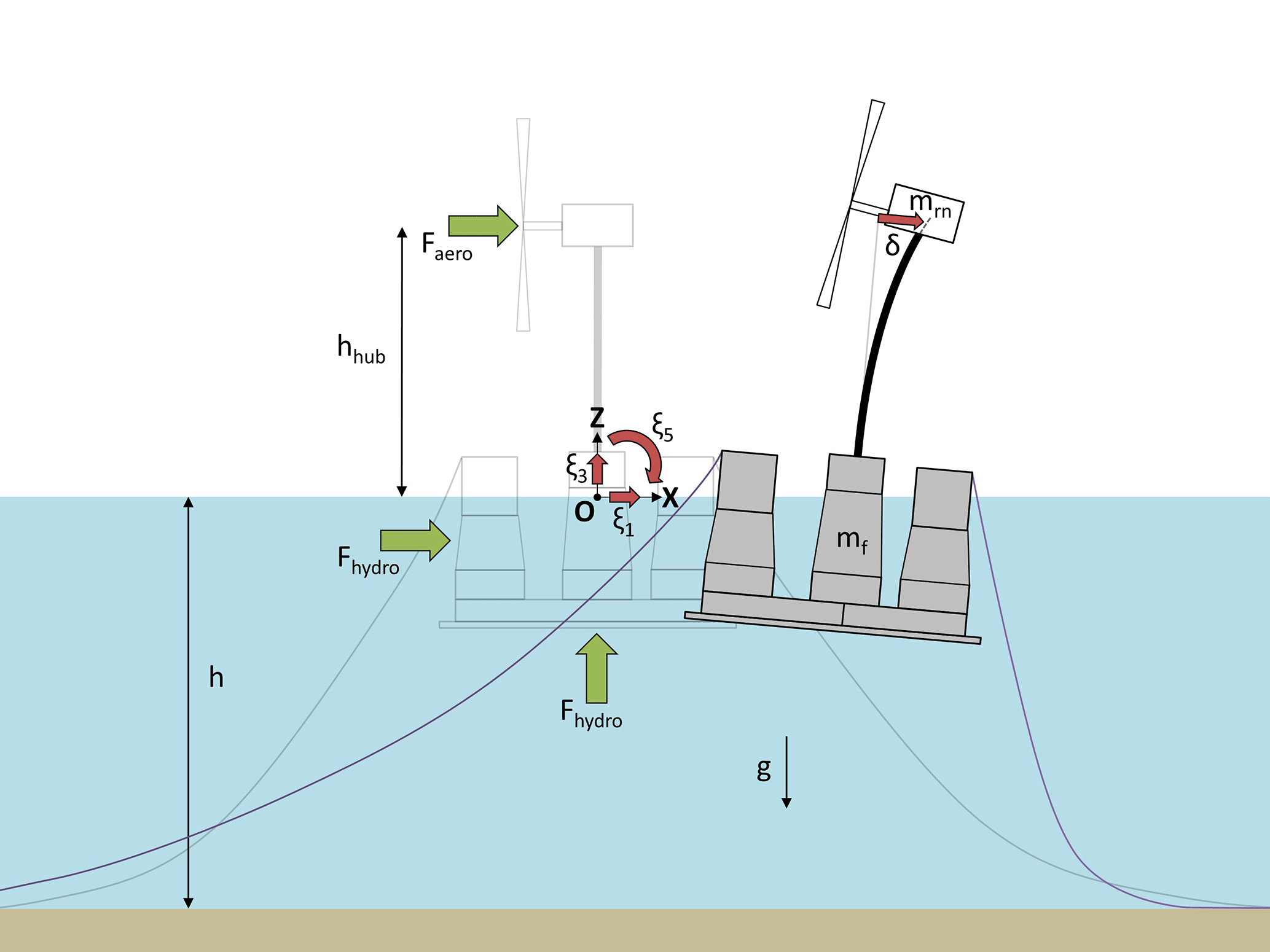
QuLAF represents the floating wind turbine as two lumped masses – floater and rotor-nacelle assembly – connected by a flexible tower. The model captures four planar DoFs – floater surge, heave, pitch and first tower fore-aft modal deflection – and is thus applicable to aligned wind and wave situations. The floating wind turbine is represented as depicted in Fig. 3. The EoM is a matrix version of Eq. (2),
where M is the structural mass and inertia matrix, A(ω) is the frequency-dependent, hydrodynamic added mass and inertia matrix, B(ω) is the frequency-dependent damping matrix, and C is the restoring matrix. The vector is the dynamic response in the frequency domain for the four DoFs and is the dynamic vector of excitation forces and moments in the frequency domain. The system transfer function is given by H(ω). The different elements in Eq. (3) are described in detail below.
5.1 Dynamic response vector
The dynamic response vector,
has one element for each DoF: floater surge, heave, pitch and first tower fore-aft modal deflection. The sign convention is that shown in Fig. 3, with positive surge in the downwind direction, positive heave upwards, positive pitch (about flotation point O) clockwise and positive tower deflection in the downwind direction. The physical tower deflection at any height z can be obtained by multiplying the mode shape ϕ(z) and the modal deflection α(t). The tower deflection at the hub height hhub is therefore given by δ(t)=ϕhubα(t). If the absolute nacelle displacement is sought, the contributions from floater surge and pitch motions must be added to the tower deflection, and the global response vector is found by introducing a transformation matrix Tglob,
5.2 Dynamic load vector
The dynamic load vector,
contains hydrodynamic loads and aerodynamic loads . Hydrodynamic loads are extracted from the solution to the diffraction problem, which provides a vector of wave excitation forces and moments in all six DoFs, namely . These excitation forces are normalized to waves of unit amplitude, therefore the wave loads for a specific time series of free-surface elevation η(t) are obtained by the product . The vector of wave excitation forces and moments is reduced to adapt it to the simplified model, and a zero is added in the fourth element for the tower DoF,
where can be computed from an input time series η(t) or from a theoretical wave spectrum. The only viscous effect considered in the model is viscous damping (see Sect. 5.8.1), but viscous forcing is neglected to keep the model computationally efficient. This simplification, however, is considered reasonable because hydrodynamics for this floater are dominated by inertia loads, and viscous forcing is expected to be relevant mainly for severe sea states, which lie on the border of the model's applicability. The vector of aerodynamic loads only contains the dynamic part of the wind loads and has the format
where and represent the horizontal and vertical components of the aerodynamic loads on the rotor, respectively. The aerodynamic tilt torque on the rotor is given by . The fourth element of represents the effect of the aerodynamic loads on the tower modal deflection, hence the mode shape deflection ϕhub and its slope ϕz,hub evaluated at the hub are involved. The time-domain aerodynamic loads for each mean wind speed W are pre-computed in the SoA model, as detailed in Sect. 5.8.2.
5.3 Structural mass and inertia matrix
The symmetric matrix of structural mass and inertia, obtained by looking at the forces needed to produce unit accelerations in the different DoFs, is defined as
where mtot is the total mass of the floating wind turbine, , which includes the mass of the floater mf, the rotor-nacelle mass mrn and the mass sum of all the Nt elements that compose the flexible tower, each with a mass per length and a height Δzi. The total mass inertia of the system about the y axis at the flotation point O is given by , including the floater inertia , the rotor-nacelle inertia and the inertia of each of the tower elements, located at an absolute height , where zt,i is the vertical position of the element i with respect to the tower base, located at a height ht. The centre of mass (CM) of the whole structure is located at , with contributions from the floater CM at , the rotor-nacelle CM at the hub height hhub and the CM of each of the tower elements. The mode shape deflection of the tower evaluated at a generic tower element i is ϕi, while ϕhub and ϕz,hub are the mode shape deflection and its slope evaluated at the hub. Finally, represents the mass inertia of the rotor-nacelle assembly referred to the tower top. The tower structural properties and first mode shape are the same as the ones given as an input to the SoA model.
5.4 Hydrodynamic added mass matrix and damping matrix
The frequency-dependent, hydrodynamic added-mass and radiation-damping matrices, A(ω) and Brad(ω), can be pre-computed in a radiation-diffraction solver. Here, the same WAMIT output files used for the SoA model are loaded into QuLAF. However, the original 6×6 matrices are reduced by removing the rows and columns corresponding to the DoFs not included in the simplified model (sway, roll, yaw), and a row and column of zeros is added for compatibility with the tower DoF,
The global damping matrix includes contributions from the hydrodynamic radiation damping Brad(ω), the hydrodynamic viscous damping Bvis, the aerodynamic damping Baero(ω) and the tower structural damping Bstruc:
The hydrodynamic viscous damping matrix Bvis is analytically extracted from the Morison equation, as shown in Section 5.8.1. The diagonal matrix of aerodynamic damping,
is extracted from the SoA model for each mean wind speed W, as detailed in Section 5.8.2. The matrix of structural damping only concerns the tower and is given by
where the structural damping ratio for the first fore-aft tower mode, ζstruc,tow, is directly taken from the input to the SoA model, and Ctow and Mtow are the last diagonal elements of the system restoring matrix C and the mass inertia matrix M, respectively.
5.5 Restoring matrix
The restoring matrix includes hydrostatic stiffness Chst, structural stiffness Cstruc and mooring stiffness Cmoor:
The hydrostatic matrix should only include the contributions from the centre of buoyancy (CB) and waterplane area. It is computed as part of the radiation-diffraction solution, and is reduced following the same procedure as for the added mass and radiation damping matrices. The symmetric matrix of structural stiffness is given by
where g is the acceleration of gravity, and EIi and ϕzz,i are the bending stiffness and the curvature of the mode shape for the tower element i, respectively. The off-diagonal term represents the negative restoring effect of the tower and rotor-nacelle mass on the tower DoF when the floater pitches. The mooring restoring matrix Cmoor is position-dependent and therefore extracted from the SoA model for each mean wind speed W, as detailed in Sect. 5.8.3. Although in this study wind is the only effect considered to affect the mean position of the floating wind turbine, other effects such as mean drift forces and current can be taken into account in the SoA model when linearizing the mooring system.
5.6 Static load and response
Static loads are related to the equilibrium of the structure. In the model, the static part of the response, ξst, is added to the dynamic part when it is converted from the frequency to the time domain via iFFT. The static loads applied are
which include the static part of the aerodynamic loads Faero,st, the gravity loads Fgrav and the buoyancy loads Fbuoy. The gravity load vector is given by
where Fmoor,z is the vertical force exerted by the mooring lines in equilibrium, and is the horizontal coordinate of the rotor-nacelle CM.
The buoyancy load vector is
where ρw is the water density, Vf is the volume displaced by the floater and is the horizontal coordinate of the floater CB. With no wind and only linear wave forcing, the floating wind turbine operates around its equilibrium position with a stiffness matrix C0. If wind (or any other mean force) is introduced, the floating wind turbine is moved to a new equilibrium position, where the stiffness matrix is CW. The static response ξst is therefore obtained from the static loads by considering a mean stiffness matrix Cst,
This approximation is accurate to second order.
5.7 System natural frequencies
The vector of natural frequencies ω0 is found by solving the undamped eigenvalue problem given by
Since the matrix of added mass depends on frequency, the eigenvalue problem is solved in a frequency loop. For each frequency ω, the four possible natural frequencies are computed. When one of the four possible frequencies obtained is equal to the frequency of that particular iteration in the loop, then a system natural frequency has been found. The system natural frequencies computed in QuLAF are compared to those obtained with the SoA model in Sect. 6.1.
5.8 Cascading techniques applied to the simplified model
In Sect. 3 it was stated that one disadvantage of frequency-domain models is their inability to directly capture loads that depend on the response in a nonlinear way. Some relevant examples are viscous drag, aerodynamic loads and catenary mooring loads. This section gives a description of the cascading methods employed to incorporate such nonlinear loads into the simplified model.
5.8.1 Hydrodynamic viscous loads
Viscous effects on submerged bodies depend nonlinearly on the relative velocity between the wave particles and the structure, hence they can only be directly incorporated in time-domain models. In the offshore community this is normally done through the drag term of the Morison equation, which provides the transversal drag force Fd on a cylindrical member section of diameter D and length dl as
where ρ is the fluid density, CD is a drag coefficient, and vf and vs are the local fluid and structure velocities perpendicular to the member axis. The equation can be also written as
which shows that the drag effects can be separated into a pure forcing term, a nonlinear damping term and a linear damping term. Since the hydrodynamics on the given floating substructure are inertia-dominated and under the assumption of small displacements around the equilibrium position, the two first terms are neglected and only the linear damping term is retained in the QuLAF model. Invoking further the assumption of small displacements and velocities relative to the fluid velocity, we have . With this assumption, the linear damping term of the viscous force becomes
A symmetric viscous damping matrix Bvis is now derived by applying Eq. (23) to the different DoFs. For the surge motion, integration over the submerged body gives the total viscous force in the x direction as
where zmin is the structure's deepest submerged point, u is the horizontal wave particle velocity and is the surge velocity. The integral in Eq. (24) requires the estimation of drag coefficients and the computation of wave kinematics at several locations on the submerged structure, which can be involved for complex geometries. These computations would reduce the CPU efficiency relative to the radiation-diffraction terms, so instead the local drag coefficient and wave velocity inside the integral are replaced by global, representative values outside the integral, CDx and urep. Hereby the force becomes
where Ax is the integral of the local diameter D over depth, or the floater's area projected on the yz plane. This defines the surge-surge element of the viscous damping matrix Bvis. Further the b51 element of the matrix is obtained by consideration of the moment from F1 around the point of flotation,
where is the first moment of area of Ax about the y axis (negative due to z≤0) and b51 is the surge-pitch element of the viscous damping matrix. In a similar way, the heave-heave and heave-pitch coefficients of Bvis are obtained by applying Eq. (23) to the heave motion,
Here is the heave velocity, w is the wave particle vertical velocity, Az is the floater's bottom area projected on the xy plane and is the first moment of area of Az about the y axis, which is zero for the present floating substructure due to symmetry. Finally, by applying Eq. (23) to the pitch motion, the pitch-pitch element of the viscous damping matrix, b55, is found. When the floater pitches with a velocity , an arbitrary point on the floater with coordinates (x,z) moves with a velocity . The motion creates a moment due to viscous effects given by
where Iy,Ax and Iy,Az are the second moments of area of Ax and Az about the y axis, respectively. The complete symmetric matrix of viscous damping is therefore
The global drag coefficients above have been chosen as CDx=1 and CDz=2, given that the bottom slab of the floater under consideration has sharp corners and is expected to oppose a greater resistance to the flow than the smooth vertical columns (see Fig. 1). To obtain the representative velocity urep, the time- and depth-dependent horizontal wave velocity at the floater's centreline is first averaged over depth and then over time,
Here k is the wave number for the angular frequency ω and h is the water depth. The representative velocity wrep is chosen as the time average of the vertical wave velocity at the centre of the bottom plate,
This simplification of the wave kinematics history, although drastic, allows for the characterization of the viscous damping for each sea state and avoids the need to compute wave kinematics locally and integrate the drag loads.
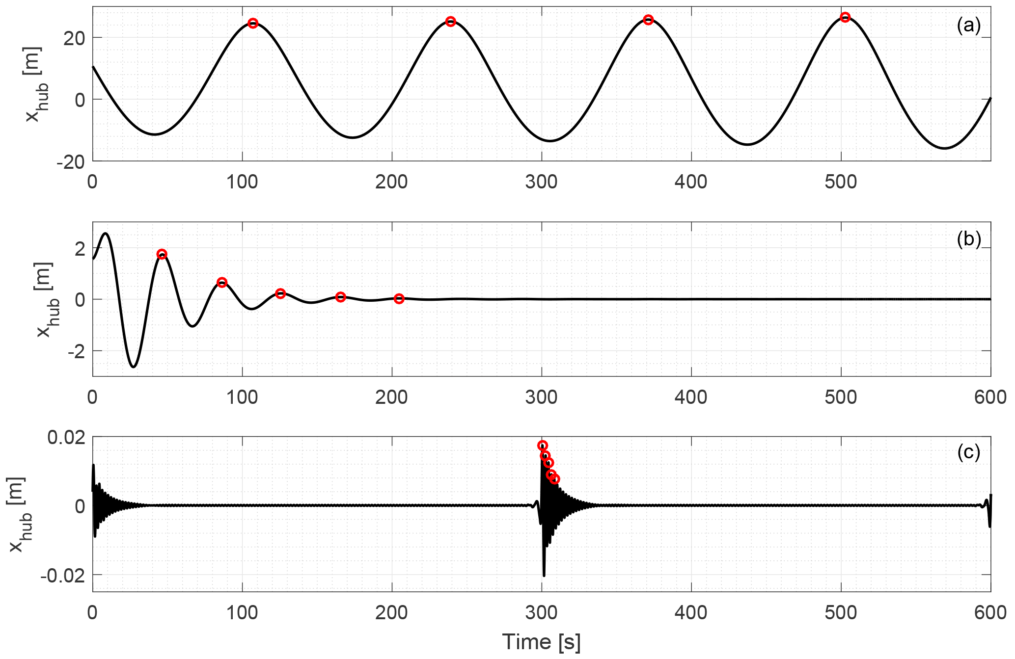
Figure 4Example of time series of hub position and selected peaks for the extraction of aerodynamic damping. From top to bottom: surge, pitch and clamped tower DoFs.
5.8.2 Aerodynamic loads
Aerodynamic loads depend on the square of the relative wind speed seen by the blades. The relative wind speed includes contributions from the rotor speed, the blade deflection, the tower deflection and the motion of the floater. The fact that the aerodynamic thrust depends on the blade relative velocity produces the well-known aerodynamic damping. State-of-the-art numerical models incorporate aerodynamic loads based on relative velocity, because both the wind speed and the blade structural velocity are known at each time step. However, this cannot be done in a frequency-domain model. In the approach implemented in QuLAF, the aerodynamic loads considering the motion of the blades are simplified and approximated by loads considering a fixed hub with rigid blades and linear damping terms. The time series of fixed-hub loads and the aerodynamic damping coefficients are extracted from the SoA model for each mean wind speed.
The aerodynamic loads are obtained at each wind speed W by a SoA simulation with turbulent wind and no waves, where all DoFs except shaft rotation and blade pitch are disabled and where the wind turbine controller is enabled. The time series of fixed-hub, pure aerodynamic loads Faero,1(t), Faero,3(t) and τaero(t) are extracted from the results and stored in a data file which is loaded into the model. Hence, these SoA simulations need to be as long as the maximum simulation time needed in the simplified model (5400 s in this case).
For a given rotor, the work carried out by the aerodynamic damping is a function of wind speed, rotational speed, turbulence intensity, motion frequency and oscillation amplitude. Here, we define an equivalent linear damping which delivers the same work over one oscillation cycle and can be extracted from a decay test. Schløer et al. (2018) used this principle for the tower fore-aft mode of a bottom-fixed offshore turbine and found that the damping was only slightly dependent of the motion amplitude. We make a further simplification and carry out the decay tests in steady wind. Since the mass and stiffness of floater and tower only affect the aerodynamic damping through the motion frequency, we transfer the damping coefficients b from the decay tests in FAST to the QuLAF model. On the contrary, if the damping ratio ζ was transferred, changes in mass or stiffness properties would imply a change in the aerodynamic forcing, which is not physically correct. With the transfer of damping coefficients b, recalculation of the decay tests is only necessary in the event that the change of natural frequencies should affect the damping values significantly. Here, the decay tests from which aerodynamic damping ratios were extracted were carried out at representative natural frequencies equal to those of the present floater. These decay tests in calm water and with the wind turbine controller active were carried out for each DoF with all the other DoFs locked. This way, the floating wind turbine was a one-DoF spring-mass-damper system in each case, where the horizontal position of the hub xhub was of interest. The decay tests were carried out as a step test in steady wind where the wind speed goes from the minimum to the maximum value with step changes every 600 s. With every step change of wind speed, the structure moves to a new equilibrium position. If all sources of hydrodynamic and structural damping are disabled, the aerodynamic damping is the only one responsible for the decay of the hub motion, and it can be extracted from the time series of xhub. The n peaks extracted from the signal are used in pairs to estimate each local logarithmic decrement di and, from it, a local damping ratio ζi, which is then averaged to obtain the aerodynamic damping ratio ζaero for the given DoF and W:
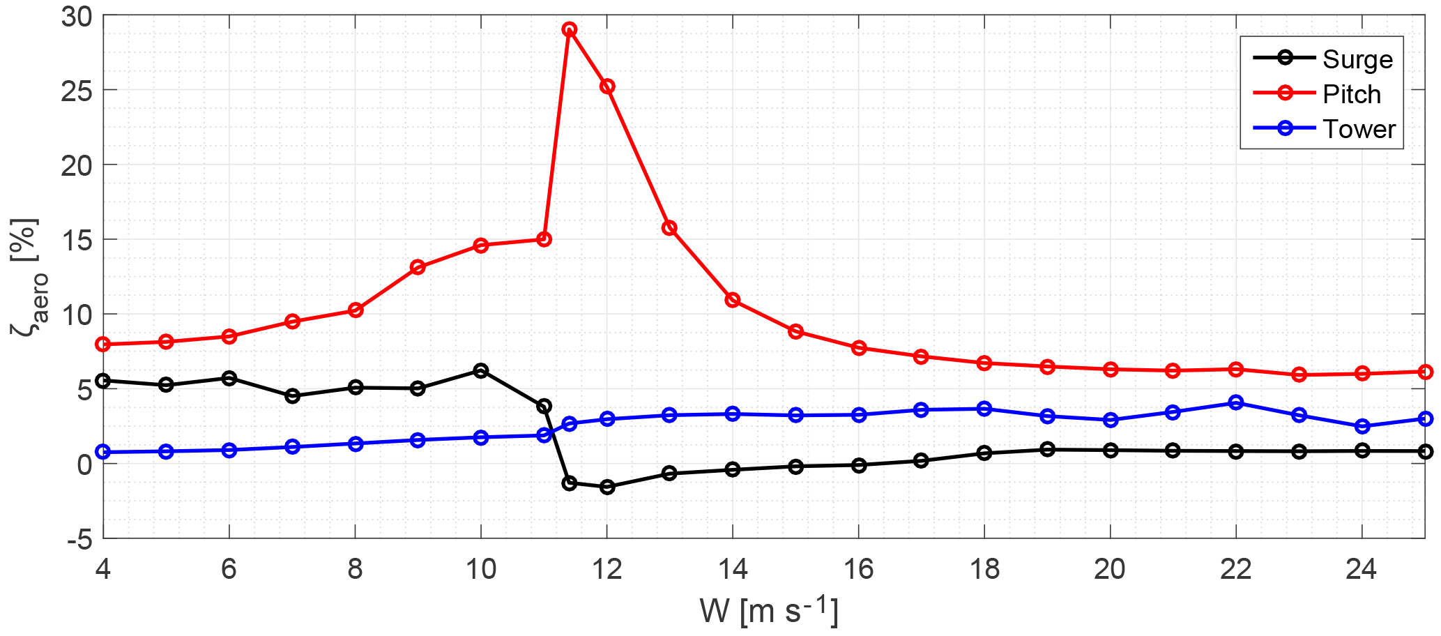
Figure 4 shows examples of xhub(t) and selected peaks for surge, pitch and clamped tower DoFs for a wind speed of 13 m s−1. The wind changed from 12 to 13 m s−1 at t=0, and the mean of the signals has been subtracted. For surge and pitch, peaks within the first 40 s are neglected to allow the unsteady aerodynamic effects to disappear. For the tower DoF, however, the frequency is much higher and the signal has died out by the time the aerodynamics are steady. For that reason, the tower decay peaks are extracted after 300 s, and a sudden impulse in wind speed is introduced at t=300 s to excite the tower. This method was chosen since the standard version of FAST does not allow an instantaneous force to be applied.
In Fig. 5 the aerodynamic damping ratio is shown for all DoFs as a function of W. It is observed that the aerodynamic damping in surge is negative for wind speeds between 11.4 and 16 m s−1, due to the wind turbine controller. However, in real environmental conditions with wind and waves, it has been observed that the hydrodynamic damping contributes to a positive global damping of the surge motion. This controller effect is similar to the “negative damping problem” reported in, for example, Larsen and Hanson (2007). The negative aerodynamic damping in surge may be eliminated if one tunes the controller natural frequency so it lies sufficiently below the surge natural frequency of the floating wind turbine, as it was done in Larsen and Hanson (2007) for the floater pitch motion. This solution, however, would make the controller too slow and would affect power production, thus it was not adopted here because the global damping in surge has been observed to be positive when all other damping contributions are taken into account.
The damping ratio for the ith DoF and each wind speed, ζaero,i(W), is next converted to a damping coefficient by
where Cii, Mii and Aii(ω) are taken from the one-DoF oscillator in the corresponding decay test. The table of aerodynamic damping coefficients as a function of wind speed baero(W) is stored in a data file, which is loaded into the model. Since the aerodynamic damping coefficients are extracted from simulations with steady wind, but applied in the model in simulations with turbulent wind, an averaging is applied to account for the variability in the wind speed in turbulent conditions. Given the time series of wind speed at hub height V(t), the probability density function (PDF) of a normal distribution given by is used to estimate the probability of occurrence within V(t) of each discrete value of W. Then the aerodynamic coefficient for the given turbulent wind conditions and the ith DoF is
5.8.3 Mooring loads
The equations that provide the loads on a catenary cable depend nonlinearly on the fairlead position. In dynamic mooring models the drag forces on the mooring cables are also included; therefore, the mooring loads also depend on the square of the relative velocity seen by the lines. These nonlinear effects can easily be captured by time-domain models, but cannot be directly accommodated in a linear frequency-domain model. In QuLAF, the mooring system is represented by a linearized stiffness matrix for each wind speed, which is extracted from the SoA model and where hydrodynamic loads on the mooring lines are neglected. The dependence of the mooring matrix on wind speed is necessary because different mean wind speeds generally produce different mean thrust forces, which displace the floating wind turbine to different equilibrium states. The stiffness of the mooring system is different at each equilibrium position because of the nonlinear force-displacement behaviour of the catenary mooring lines.
For each wind speed a first SoA simulation is needed with steady, uniform wind and no waves, where only the tower fore-aft and floater surge, heave and pitch DoFs are enabled. After some time the floating wind turbine settles at its equilibrium position , which is stored. These simulations should be just long enough so that the equilibrium state is reached (600 s in this case). Then, a new short SoA simulation with all DoFs disabled is run, where the floater initial position is the equilibrium with a small positive perturbation in surge, . This simulation should be just long enough for the mooring lines to settle at rest (120 s in this case). The global mooring forces in surge and heave and the global mooring moment in pitch are stored, namely . The process is repeated now with a negative perturbation in surge , giving . All this information is enough to compute the first column of the mooring matrix Cmoor for the wind speed W. Perturbations in heave ±Δξ3 and pitch ±Δξ5 provide the necessary information to compute the rest of the columns, and therefore the full matrix:
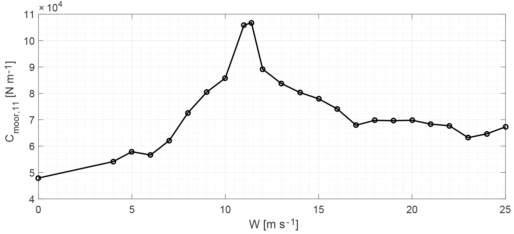
The first element of the mooring matrix Cmoor,11 is shown as a function of wind speed in Fig. 6. It is observed that the stiffness in surge reaches its maximum around rated wind speed (11.4 m s−1), where the thrust is also maximum and the floating wind turbine is the furthest from the equilibrium position with no wind.
In the method applied here the linearization of the mooring system has been done with the SoA model. However, in a real design study where the mooring characteristics change, the above procedure can be made significantly faster by direct static analysis of the nonlinear mooring reactions around the floater equilibrium positions.
5.9 Estimation of extreme responses: a spectral approach
Classical Monte Carlo analysis of response to stochastic loads entails running a simulation, extracting the peaks from the response time series, sorting them in ascending order and assigning an exceedance probability to each peak based on their position in the sorted list. Several simulations of the same environmental conditions with different random seeds provide a family of curves in the exceedance probability plot, which can be used to estimate the expected response level for a given exceedance probability. We note that the extracted exceedance probability curves are based on the assumption that the peaks are independent, which may not always be the case. Yet, in this section the linear nature of the simplified model will be further exploited to obtain an estimation of the extreme responses to wave loads by solely using the wave spectrum and the system transfer function, thus eliminating the need for a response time series and the bias introduced by a particular random seed. An extension of the method to wind and wave forcing is further presented and discussed.
In a Gaussian, narrow-banded process, the peaks follow a Rayleigh distribution. In linear stochastic sea states, the free-surface elevation η(t) is a Gaussian random variable Rη with zero mean. Thus, within the narrow-banded assumption, which often applies to good approximation, the crest heights follow a Rayleigh distribution (Longuet-Higgins, 1956) given by
where the variance in η(t) is , which can be obtained from the integral of the wave spectrum,
If we only consider linear wave forcing, the response is also Gaussian for the linear system in Eq. (3). If the response is also narrow-banded, its exceedance probability can be found via the standard deviation of the response, which in turn can be obtained by integration of the response spectrum. From Eq. (3) we have
where TFη→ξ(ω) is a direct transfer function from surface elevation to global response. The global response spectra Sξ,glob(ω) is related to the wave spectrum Sη(ω) in a similar way (Naess and Moan, 2013),
Here *T indicates the transpose and complex conjugate. By virtue of Eq. (37), the exceedance probability of, for example, the surge response ξ1 is known from the variance in the surge response , which is given by
For nacelle acceleration we can write the response as a function of the global nacelle displacement ξglob,4; therefore,
The turbulent part of the wind speed can also be considered a Gaussian random variable (Longuet-Higgins, 1956). On the other hand, aerodynamic loads are not a linear function of wind speed. Therefore the response to wind loads cannot be assumed to be Gaussian, and the approach shown above is not valid. However, the method above can be applied to cases with wind and wave forcing, bearing in mind that the results may not be accurate since the necessary assumptions are not fulfilled. If wind and wave forcing are considered, Eq. (3) can be written as
where TFF→ξ(ω) is a direct transfer function from load to global response. The global response spectra Sξ,glob(ω) is now given by (Naess and Moan, 2013)
Here SF(ω) is the spectra of the total loads (hydrodynamic and aerodynamic),
This method provides the exceedance probability of the dynamic part of the response, therefore the static part should be added after applying Eq. (37). Exceedance probability results from this method are compared in the next section to the traditional way of peak extraction from response time series.
5.10 Integration of QuLAF in optimization loops
The main purpose of QuLAF is to provide a quick assessment of loads, response and natural frequencies early in the design phase, where several variations of the baseline design are to be evaluated. The efficiency in the model is achieved by (i) considering only a few DoFs; (ii) solving the linear EoMs in the frequency domain; and (iii) pre-computing the aerodynamic loads and aerodynamic damping coefficients. The application of the model to an optimization loop can be divided into two stages: a preparation stage, which needs to be done only once for a given baseline floating wind turbine, and a calculation stage, which can be repeated for each variation in the baseline design. After the optimal design has been found through optimization, it should be verified by running a complete load basis in a SoA model.
-
Preparation stage. Once the wind turbine, the baseline floater design and the design basis are defined, the preparation stage entails the following.
-
Computation of time series of aerodynamic loads at the shaft for the needed wind speeds and turbulence random seeds, considering rigid blades and fixed nacelle. The wind turbine controller should be active and tuned according to the pitch frequency of the baseline design.
-
Extraction of aerodynamic damping coefficients for the needed wind speeds, by carrying out decay tests in steady wind of the surge, pitch and clamped tower DoFs.
-
Storage of the aerodynamic loads and damping coefficients in a database that can be reused for several candidate designs.
-
-
Calculation stage. The calculation stage is done for each candidate design in the pre-design optimization loop by following these steps.
-
Computation of the radiation-diffraction solution in, for example, WAMIT.
-
Extraction of structural mass and stiffness properties.
-
For each wind speed, calculation of the equilibrium position and linearization of the mooring system around it.
-
Prediction of the natural frequencies, response and loads for several environmental conditions using QuLAF.
-
When compared to the same number of simulations in the SoA model, the advantage of the simplified model resides in the low computational cost of applying the calculation step 4 to several environmental conditions and different variations in the baseline design. The extra work needed to achieve the speed up comes from the aerodynamic pre-computations in the preparation stage and from the linearization of the mooring system (step 3) in each iteration of the calculation stage. However, the aerodynamic loads need to be extracted from the SoA model only once for a given wind turbine, while the aerodynamic damping coefficients can also be reused for different variations of the baseline floating wind turbine, provided that the system natural frequencies do not change significantly between different design iterations. The linearization of the mooring system and the computation of the radiation-diffraction solution may also be automated. Alternatively, for slender, simpler geometries (such as spars), a Morison approach may be implemented in QuLAF, thus eliminating step 1 in the calculation stage. For the present study, however, the radiation-diffraction solution was chosen due to the shape and size of the floating substructure in consideration, and a comparison to the Morison-based alternative has not been conducted.
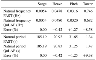
Table 3Natural frequencies and periods obtained in FAST and QuLAF.
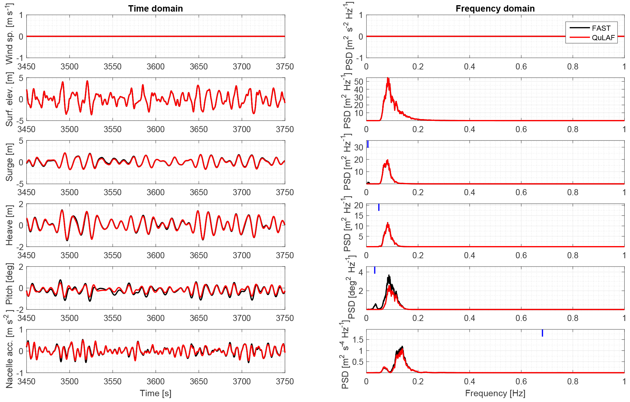
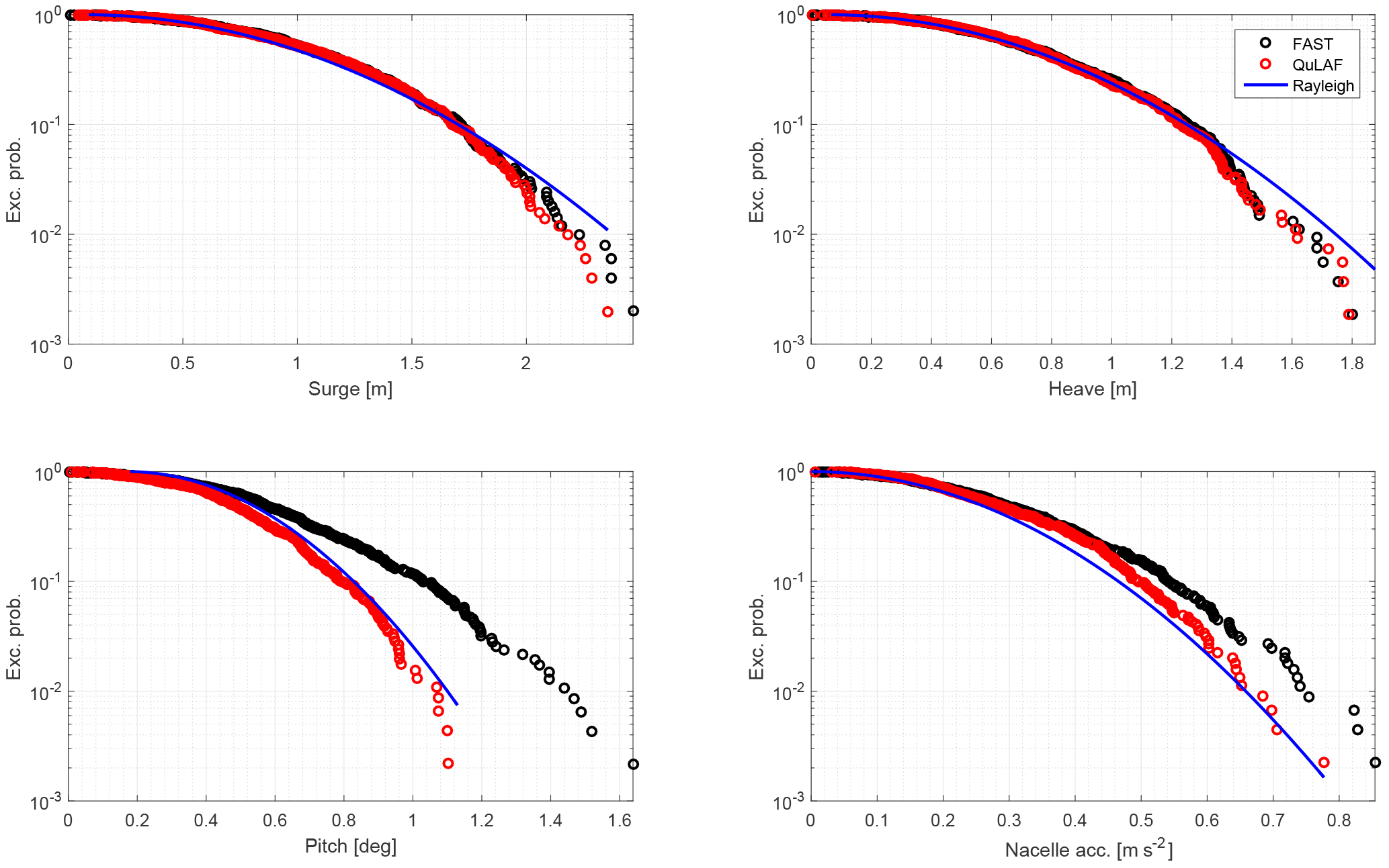
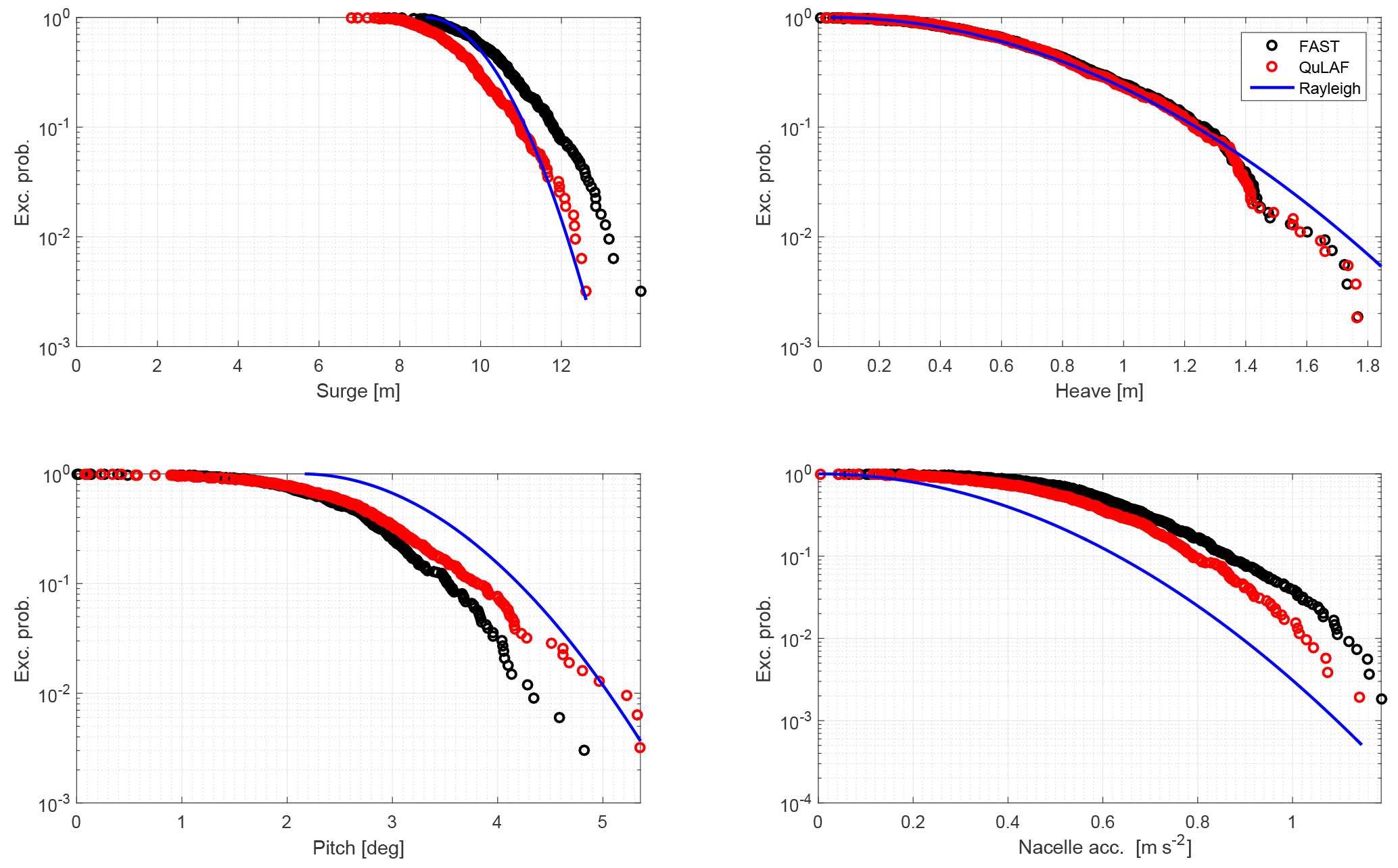
We now compare and discuss the QuLAF and FAST responses to the same environmental conditions (see Table 4) representative of the Gulf of Maine (Krieger et al., 2015). The cases considered include five irregular sea states with and without turbulent wind, with a single realization for each sea state. In all cases the total simulated time was 5400 s in both models. The first 1800 s were neglected to discard initial transient effects in the time-domain model. The free-surface elevation of irregular sea states was computed in FAST from a Pierson–Moskowitz spectrum, and the turbulent wind fields in TurbSim from an IEC Kaimal spectrum. Since the turbulent wind fields used in the SoA simulations are the same employed for the pre-computation of aerodynamic loads, and the free-surface elevation signal in the cascaded model is also taken from the FAST simulation, a deterministic comparison of time series is possible for all cases. In the plots shown in this section (Figs. 7 and 9), the left-hand side shows a portion of the time series of wind speed at hub height, free-surface elevation, floater surge, heave and pitch, and nacelle acceleration; and the right-hand side shows the PSDs of the same signals. The PSD signals were smoothened with a moving-average filter of 20 points to ease the spectral comparison between models. The short blue vertical lines in the PSD plots indicate the position of the system natural frequencies predicted by the simplified model (see Table 3). In addition, exceedance probability plots of the responses with both models are shown (Figs. 8 and 10), based on peaks extracted from the time series. The peaks were sorted and assigned an exceedance probability based on their position in the sorted list. The exceedance probability of the extracted peaks is compared to the one estimated with the method described in Sect. 5.9, labelled as “Rayleigh”.
6.1 System identification
The system natural frequencies were calculated in QuLAF by solving the eigenvalue problem in Eq. (20). In FAST, decay simulations were carried out with all DoFs active, where an initial displacement was introduced in each relevant DoF and the system was left to decay. A PSD of the relevant response revealed the natural frequency of each DoF. A comparison of natural frequencies and periods found with the two models is given in Table 3, where it is shown that all floater natural frequencies in the simplified model are within 1.3 % error compared to the SoA model. On the other hand, the tower frequency is 8.6 % below the one estimated in FAST. This difference is due to the absence of flexible blades in the simplified model, which are known to affect the coupled tower natural frequency. With rigid blades, the SoA model predicts a coupled tower natural frequency of 0.684 Hz, only 0.3 % above the tower frequency in QuLAF.
The model presented here may be calibrated against other numerical or physical models if needed, by introducing user-defined additional restoring and damping matrices. For the present study, however, no calibration against the SoA model was applied, in order to keep the model calibration free and assess its suitability for optimization loops.
6.2 Response to irregular waves
The response to irregular waves with Hs=6.14 m and Tp=12.5 s (case “Waves 5” in Table 4) is shown in Fig. 7. On the frequency side, all motions show response mainly at the wave frequency range, and there is a very good agreement between both models for surge and heave. In pitch – and consequently in nacelle acceleration – the QuLAF model shows a lower level of excitation at the wave frequency range when compared to FAST. This deviation was traced to the absence of viscous forcing in the simplified model, since the two pitch responses are almost identical if viscous effects are disabled in both models. As expected, the agreement is better for milder sea states, where viscous forcing is less important. In surge and pitch some energy is visible at the natural frequencies, but only in the FAST model. Since the peaks lie out of the wave spectrum and are not captured by QuLAF, they could originate from nonlinear mooring effects or from the drag loads, which are also nonlinear.
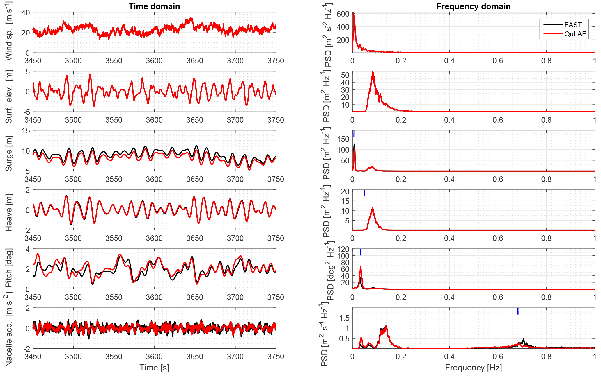
Figure 8 shows exceedance probability plots of the response to irregular waves. The Rayleigh curves fit well to the responses given by the simplified model, which is expected, given that the free-surface elevation and the hydrodynamic forcing are linear in the model, and the response can be considered narrow-banded. In the comparison between the two models, the surge and heave peaks are very well estimated by QuLAF. In nacelle acceleration and especially in pitch, however, the model underpredicts the response, with a difference of about 30 % in pitch and about 8 % in nacelle acceleration for the largest peak when compared to FAST. These observations in extreme response are consistent with the spectral results of Fig. 7 discussed above.
6.3 Response to irregular waves and turbulent wind
The response to irregular waves with Hs=6.14 m and Tp=12.5 s and turbulent wind at W=22 m s−1 (case “Waves + wind 5” in Table 4) is shown in Fig. 9. The surge motion is dominated by the surge natural frequency, which is clearly excited by the wind forcing. The linear model slightly underpredicts this resonance of the wind forcing with the surge natural frequency. Heave is dominated by the wave forcing, and the response of both models agree well. In pitch, resonance with the natural frequency also exists in both models, although QuLAF predicts more energy at that frequency than FAST. Both surge and pitch responses are resonant, thus they are especially sensitive to the amount of damping. The overprediction of pitch motion also leaves a footprint on the PSD of nacelle acceleration, which shows energy at the pitch natural frequency, the wave frequency range and the tower natural frequency. The level of excitation of the tower mode at 0.682 Hz, however, is slightly underpredicted by QuLAF, likely due to an overestimation of the aerodynamic damping on the tower DoF.
The associated exceedance probability plots are shown in Fig. 10. In this case the Rayleigh curves generally do not fit the responses predicted by the linear model, as the extreme peaks are no longer Rayleigh-distributed. This is because the nonlinear nature of the wind loads makes the response non-Gaussian, and in some cases broad-banded with distinct frequency bands excited (e.g. the tower response cannot be considered narrow-banded here). The best fit is seen for heave, which is mainly excited by linear wave loads and is also narrow-banded. When compared to FAST, however, QuLAF shows a good agreement with errors in the largest response peaks of approximately 8 % in surge, 12 % in pitch and 4 % in nacelle acceleration.
6.4 Comparison of fatigue damage-equivalent loads
Table 4 shows a summary of fatigue DELs for a wider range of environmental conditions. Each case is defined by the significant wave height Hs, the wave peak period Tp and the mean wind speed W. The fatigue damage-equivalent bending moment at the tower base estimated with the two models is presented, as well as the error for the simplified model. Finally, the last column shows the ratio between the simulated time and the CPU time in QuLAF, Trel. The cases labelled as “5” correspond to the results discussed in the previous section. The two DEL columns in Table 4 are also shown in Fig. 11 as a bar plot.
Table 4Summary of environmental conditions (Krieger et al., 2015) and DEL results obtained in FAST and QuLAF.
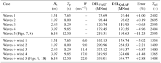
For the cases with waves only, the model underpredicts the DEL at the tower base with errors from 0.2 % to 11.3 % that increase with the sea state, as observed in Fig. 11. The significant wave height also increases with the sea state, as do the associated nonlinear effects of position-dependent mooring stiffness and viscous hydrodynamic forcing, which are both included in FAST. QuLAF does not include viscous hydrodynamic forcing, and as a linear model, its accuracy is bound to the assumptions of small displacements around the equilibrium point. Hence, it is expected that the linear model performs worse for the environmental conditions where nonlinear effects are not negligible. This observation is also consistent with the discussion around Fig. 7, which corresponds to the most severe sea state considered here.

Figure 11Damage-equivalent bending moment at the tower base for different environmental conditions.
For the cases with wind, the errors range from 1.5 % to 6.9 %, but the trend is not as clear. The predictions seem to be worst for the environmental condition corresponding to rated wind speed. Around rated speed the wind turbine operation switches between the partial- and the full-load regions, which correspond to very distinct regimes of the generator torque and blade pitch controller. The complexity of the dynamics involved in this transition zone is not well captured by the simplified model. The vibration of the tower is also more likely to be excited around rated wind speed, where the thrust is maximum. As the coupled tower natural frequency is different for the two models, this will also have an impact on the resulting DEL. This effect has been quantified for rated wind speed (”Waves + wind 3”), where the DEL error becomes −5.6 % when the FAST simulation is carried out with rigid blades, which indicates that the difference in coupled tower frequency has some impact on the DEL error. In addition, the aerodynamic damping – which plays an important role in the resonant response of the tower – is dependent on the frequency at which the rotor moves in and out of the wind. Since the aerodynamic damping on the tower is extracted from a SoA simulation with fixed foundation and rigid blades, it corresponds to a tower natural frequency of 0.51 Hz, different to the coupled tower frequency observed when the floater DoFs are active (0.682 Hz in QuLAF, 0.746 in FAST). This difference in the frequencies at which the aerodynamic damping is extracted and applied is likely to lead to an overprediction of the aerodynamic damping, and an underprediction of the tower vibration and the DEL. This observation is consistent with the level of tower response at the coupled tower frequency shown in Fig. 9. On the other hand, the aerodynamic simplifications in the cascaded model seem to work best for wind speeds above rated, likely due to the thrust curve being flatter in this region. The last column of Table 4 shows that the ratio between simulated time and CPU time is between 1300 and 2700 for a standard laptop with an Intel Core i5-5300U processor at 2.30 GHz and 16 GB of RAM. In other words, all the simulations in Table 4 together, 1.5 h long each, can be done in about half a minute.
A model for Quick Load Analysis of Floating wind turbines, QuLAF, has been presented and validated. The model is a linear, frequency-domain tool with four planar degrees of freedom (DoFs): floater surge, heave, pitch and tower modal deflection. The model relies on higher-fidelity tools from which hydrodynamic, aerodynamic and mooring loads are extracted and cascaded. Hydrodynamic and aerodynamic loads are pre-computed in WAMIT and FAST, respectively, while the mooring system is linearized around the equilibrium position for each wind speed using MoorDyn. A simplified approach for viscous hydrodynamic damping was implemented, and the decay-based extraction of aerodynamic damping of Schløer et al. (2018) was extended to multiple DoFs. Without introducing any calibration, a case study with a semi-submersible 10 MW configuration showed that the model is able to predict the motions of the system in stochastic wind and waves with acceptable accuracy. The damage-equivalent bending moment at the tower base is estimated with errors between 0.2 % and 11.3 % for all the five load cases considered in this study, covering the operational wind speed range. The largest errors were observed for the most severe wave climates in wave-only conditions and for turbine operation around rated wind speed for combined wind and wave conditions, due to three main limitations in the model: (i) underprediction of hydrodynamic loads in severe sea states due to the omission of viscous drag forcing; (ii) difficulty to capture the complexity of aerodynamic loads around rated wind speed, where the controller switches between the partial- and full-load regions; and (iii) errors in the estimation of the tower response due to underprediction of the coupled tower natural frequency and overprediction of the aerodynamic damping on the tower. The computational speed in QuLAF is between 1300 and 2700 times faster than real time. Although not done in this study, introducing viscous hydrodynamic forcing and calibration of the damping against the SoA model would likely result in improved accuracy, but at the expense of lower CPU efficiency and less generality in the model formulation.
It has been shown that the model can be used as a tool to explore the design space in the preliminary design stages of a floating substructure for offshore wind. The model can quickly give an estimate of the main natural frequencies, response and loads for a wide range of environmental conditions with aligned wind and waves, which makes it useful for optimization loops. Although a better performance may be achieved through calibration, a calibration-free approach was used here to emulate the reality of an optimization loop, where calibration is not possible. In such a process, once an optimized design has been found, a full aero-hydro-servo-elastic model is still necessary to assess the performance in a wider range of environmental conditions, including nonlinearities, transient effects and real-time control. Since the model is directly extracted from such a SoA model, this step can readily be taken. While the SoA model should thus still be used in the design verification, the present model provides an efficient and relatively accurate complementary tool for rational engineering design of offshore wind turbine floaters. In addition, the QuLAF and FAST models presented in this study have been recently used in the LIFES50+ project for a broader analysis of different design-driving load cases, including normal operation, extreme and transient events (Madsen et al., 2018). Generally, the results of the broader study and the conclusions drawn are aligned with the ones presented here, as well as the limitations observed in the simplified model when compared to its SoA counterpart.
Given the model limitations observed in this study and in Madsen et al. (2018), possible improvements of QuLAF may involve (i) inclusion of viscous drag forcing, (ii) modelling the effect of blade flexibility on the tower natural frequency, (iii) improvement of the extraction of aerodynamic damping from the SoA model, and (iv) extension of the model to out-of-plane DoFs to make it applicable to cases with misaligned wind and waves.
The FAST model is publicly available, as detailed in Pegalajar-Jurado et al. (2018a) and Pegalajar-Jurado et al. (2018b). The QuLAF source code is not public due to possible commercialization in the future. The data used in figures and tables can be obtained by contacting the first author.
APJ is the main responsible person for developing the simplified model, carrying out the simulations, analysing the results and preparing the manuscript. MB provided input to the model development and to the first version of the manuscript. HB developed the conceptual idea, provided input to the model development and reviewed the paper in all its versions.
The authors declare that they have no conflict of interest.
This work was carried out as part of the LIFES50+ project
(http://www.lifes50plus.eu; last access: 16 February 2018). The
research leading to these results has received funding from the European
Union's Horizon 2020 research and innovation programme under grant agreement
no. 640741. Also, the authors are grateful to Dr.techn. Olav Olsen AS
(http://www.olavolsen.no; last access: 24 November 2017) for the
permission to use their concept of the OO-Star Wind Floater Semi 10 MW as the
case study.
Edited by: Joachim
Peinke
Reviewed by: Tor Anders Nygaard and one anonymous
referee
Bak, C., Zahle, F., Bitsche, R., Kim, T., Yde, A., Henriksen, L., Natarajan, A., and Hansen, M.: Description of the DTU 10 MW reference wind turbine, Tech. Rep., No. I-0092, DTU Wind Energy, 2013. a, b, c
Cummins, W.: The impulse response functions and ship motions, Schiffstechnik, 9, 101–109, 1962. a
DNV-GL AS: Bladed, https://www.dnvgl.com/energy/generation/software/bladed/index.html (last access: 5 Decemebr 2017), 2016. a
Hall, M.: MoorDyn, http://www.matt-hall.ca/moordyn.html (last access: 5 December 2017), 2017. a, b
Hansen, M.: Aerodynamics of wind turbines, Earthscan Publications Ltd., 2nd Edn., 2008. a
Hansen, M. and Henriksen, L.: Basic DTU Wind Energy controller, Tech. Rep., No. E-0028, DTU Wind Energy, 2013. a
Jonkman, J.: Dynamics of offshore floating wind turbines – Model development and verification, Wind Energy, 12, 459–492, https://doi.org/10.1002/we.347, 2009. a
Jonkman, J.: Definition of the floating system for Phase IV of OC3, Tech. Rep., No. NREL/TP-500-47535, National Renewable Energy Laboratory, 2010. a, b, c, d
Jonkman, J. and Jonkman, B.: NWTC Information Portal (FAST v8), https://nwtc.nrel.gov/FAST8 (last access: 5 December 2017), 2016. a, b
Krieger, A., Ramachandran, G., Vita, L., Gómez-Alonso, G., Berque, J., and Aguirre, G.: LIFES50+ D7.2: Design basis, Tech. rep., DNV-GL, 2015. a, b
Larsen, T. and Hanson, T.: A method to avoid negative damped low frequent tower vibrations for a floating, pitch controlled wind turbine, J. Phys. Conf. Ser., 75, 012073, https://doi.org/10.1088/1742-6596/75/1/012073, 2007. a, b, c
Lee, C. and Newman, J.: WAMIT, http://www.wamit.com/, 2016. a, b
Lemmer, F., Raach, S., Schlipf, D., and Cheng, P.: Parametric wave excitation model for floating wind turbines, Energy Proced., 94, 290–305, https://doi.org/10.1016/j.egypro.2016.09.186, 2016. a
Longuet-Higgins, M.: Statistical properties of a moving waveform, P. Camb. Philol. S., 52, 234–245, https://doi.org/10.1017/S0305004100031224, 1956. a
Lupton, R.: Frequency-domain modelling of floating wind turbines, Ph.D. thesis, University of Cambridge, 2014. a
Madsen, F., Pegalajar-Jurado, A., Bredmose, H., Borg, M., Müller, K., and Matha, D.: LIFES50+ D7.8: Required numerical model fidelity and critical design load cases in various design phases, Tech. Rep., Technical University of Denmark, 2018. a, b
Morison, J., Johnson, J., and Schaaf, S.: The force exerted by surface waves on piles, J. Petrol. Technol., 2, 149–154, https://doi.org/10.2118/950149-G, 1950. a
Naess, A. and Moan, T.: Stochastic dynamics of marine structures, Cambridge University Press, 1st Edn., 2013. a, b
Newman, J.: Marine hydrodynamics, The MIT Press, 3rd Edn., 1980. a
Øye, S.: FLEX4 simulation of wind turbine dynamics, in: Proceedings of the 28th IEA meeting of experts concerning state of the art of aero-elastic codes for wind turbine calculations, 1996. a
Pegalajar-Jurado, A., Bredmose, H., and Borg, M.: Multi-level hydrodynamic modelling of a scaled 10MW TLP wind turbine, Energy Proced., 94, 124–132, https://doi.org/10.1016/j.egypro.2016.09.206, 2016. a
Pegalajar-Jurado, A., Bredmose, H., Borg, M., Straume, J., Landbø, T., Andersen, H., Yu, W., Müller, K., and Lemmer, F.: State-of-the-art model for the LIFES50+ OO-Star Wind Floater Semi 10MW floating wind turbine, J. Phys. Conf. Ser., in press, 2018a. a
Pegalajar-Jurado, A., Madsen, F., Borg, M., and Bredmose, H.: LIFES50+ D4.5: State-of-the-art models for the two LIFES50+ 10 MW floater concepts, Tech. rep., Technical University of Denmark, 2018b. a
Robertson, A., Jonkman, J., Masciola, M., Song, H., Goupee, A., Coulling, A., and Luan, C.: Definition of the semisubmersible floating system for Phase II of OC4, Tech. rep., No. NREL/TP-5000-60601, National Renewable Energy Laboratory, 2014. a, b
Schløer, S., Garcia Castillo, L., Fejerskov, M., Stroescu, E., and Bredmose, H.: A model for quick load analysis for monopile-type offshore wind turbine substructures, Wind Energ. Sci., 3, 57–73, https://doi.org/10.5194/wes-3-57-2018, 2018. a, b, c
van der Tempel, J.: Design of support structures for offshore wind turbines, Ph.D. thesis, Delft University of Technology, 2006. a, b
Wang, K., Ji, C., Xue, H., and Tang, W.: Frequency domain approach for the coupled analysis of floating wind turbine system, Ships and Offshore Struct., 12, 767–774, https://doi.org/10.1080/17445302.2016.1241365, 2017. a
Yu, W., Müller, K., and Lemmer, F.: LIFES50+ D4.2: Public definition of the two LIFES50+ 10 MW floater concepts, Tech. rep., University of Stuttgart, 2018. a, b, c
- Abstract
- Introduction: the need for an efficient, frequency-domain tool
- The case study
- Time vs. frequency domain: advantages and disadvantages
- The time-domain, state-of-the-art numerical model
- The frequency-domain, cascaded numerical model
- Validation of the QuLAF model
- Conclusions
- Code and data availability
- Author contributions
- Competing interests
- Acknowledgements
- References