the Creative Commons Attribution 4.0 License.
the Creative Commons Attribution 4.0 License.
 | 22 May 2019
Local turbulence parameterization improves the Jensen wake model and its implementation for power optimization of an operating wind farm
Olivier Coupiac
Nicolas Girard
Gregor Giebel
Tuhfe Göçmen
In this paper, a new calculation procedure to improve the accuracy of the Jensen wake model for operating wind farms is proposed. In this procedure, the wake decay constant is updated locally at each wind turbine based on the turbulence intensity measurement provided by the nacelle anemometer. This procedure was tested against experimental data at the Sole du Moulin Vieux (SMV) onshore wind farm in France and the Horns Rev-I offshore wind farm in Denmark. Results indicate that the wake deficit at each wind turbine is described more accurately than when using the original model, reducing the error from 15 % to 20 % to approximately 5 %. Furthermore, this new model properly calibrated for the SMV wind farm is then used for coordinated control purposes. Assuming an axial induction control strategy, and following a model predictive approach, new power settings leading to an increased overall power production of the farm are derived. Power gains found are on the order of 2.5 % for a two-wind-turbine case with close spacing and 1 % to 1.5 % for a row of five wind turbines with a larger spacing. Finally, the uncertainty of the updated Jensen model is quantified considering the model inputs. When checked against the predicted power gain, the uncertainty of the model estimations is seen to be excessive, reaching approximately 4 %, which indicates the difficulty of field observations for such a gain. Nevertheless, the optimized settings are to be implemented during a field test campaign at SMV wind farm in the scope of the national project SMARTEOLE.
- Article
(5005 KB) - Full-text XML
- BibTeX
- EndNote


Wind turbines are aggregated together in wind farms to take advantage of economies of scale and reduce overall costs (Pao and Johnson, 2009). However, this creates wake interactions between the turbines which are responsible for an increase in mechanical loads and a decrease in power production. It is generally not possible to avoid completely these interactions due to constraints imposed on the development of wind farms, and moreover in some cases wake effects are still persistent at significant distances downstream, up to 10 to 15 diameters (Sanderse, 2009).
To reduce these effects and improve wind farm efficiency and sustainability, wind farm coordinated control strategies are currently investigated. Contrary to the state-of-the-art control, in which all turbines maximize their own power production, coordinated control aims at controlling turbines at a wind farm scale to optimize its overall output. Two different strategies are mainly considered to achieve this goal: either the upwind turbines are curtailed to leave more kinetic energy downstream or they are yawed to deflect the wake away from the downwind turbines.
Results from simulations show that small gains in power production are indeed possible (Bossanyi and Jorge, 2016; Gebraad et al., 2017; Santhanagopalan et al., 2018); however, they also underline their high variability with incoming wind conditions (Knudsen et al., 2015). It is therefore not known to what extent these gains can be reproduced in an operating wind farm where wind conditions are fluctuating constantly and significantly. Very few full-scale field tests have been realized to investigate this question. The concepts of “heat and flux” (Machielse et al., 2007) and “controlling wind” (Wagenaar et al., 2012) were studied some years ago at the Energy research Centre of the Netherlands (ECN) and more recently the National Renewable Energy Laboratory (NREL) provided in Fleming et al. (2017) a field test of their “yaw-based wake steering” method in an Envision offshore wind farm. They tend to confirm that gains can be achieved in practice; however, in all cases, uncertainties remain high, and it is therefore difficult to give a definite conclusion.
Other full-scale field tests are currently being held in France in the scope of the French national project SMARTEOLE. They are organized in an operating wind farm owned by ENGIE Green, Sole du Moulin Vieux (SMV), in which different curtailment and yaw offset strategies are studied. The main objective of these tests is to investigate the relevance of these strategies on wind turbine power production and loads, and determine whether they could prove beneficial when applied on commercial wind farms. A first experiment campaign was realized between December 2015 and April 2016 and was dedicated to axial induction control strategy. An intentionally high level of curtailment was applied on a wind turbine of the farm so that changes in its emitted wake could be observed from the analysis of downstream active power data. Even though no increase in aggregated power production was expected, a first analysis of wind turbine power production in the farm showed that part of the lost power at the upstream turbine could be retrieved downstream (Ahmad et al., 2017; Duc, 2017).
The goal of this paper is to use the knowledge gained during the first campaign to provide new optimized control commands that could be implemented in a second field campaign and hopefully lead to an increase in the aggregated power production of the farm. As SMV is a commercial wind farm, these commands must be easily applicable without modifying the wind turbine control system; thus, a model predictive approach is followed to determine the optimal de-rating to be applied as a function of wind speed and direction. To limit computational costs and the complexity of the optimization process, fast and simple models are considered. Hence, simplified engineering models are to be applied and the main issue when following this kind of approach is making sure that they are accurately capturing the wake deficit at each wind turbine. Consequently, the data recorded during the first field test campaign are analysed further and used to propose a new tuning of the widely used Jensen model (Jensen, 1983; Katic et al., 1986). In this new method, the wake decay constant is expressed at each wind turbine based on the local measurement of turbulence intensity provided by the nacelle anemometer. The resulting wake deficit appears to be more consistent with the observed data at SMV wind farm than when using a constant value, and this calculation procedure is also validated considering experimental data from the Horns Rev-I offshore wind farm.
The rest of this paper is organized as follows. In Sect. 2, the wind farm and the experimental setup used during the first field test campaign are shortly detailed. Section 3 describes the principle of the tuned Jensen model, and its performance compared to the original model is assessed in Sect. 4. This tuned model is then used in Sect. 5 alongside a simple cT estimation procedure to predict in two study cases at SMV wind farm the optimized settings leading to an increase in overall wind farm production. Uncertainty of the model estimation is also quantified in this section and constraints related to field implementation are briefly discussed. Finally, Sect. 6 provides a summary of the paper and conclusions.
Sole du Moulin Vieux is a commercial wind farm owned by ENGIE Green and located at Ablaincourt-Pressoir in the region Hauts-de-France, approximately midway between Paris and Lille. Figure 1 shows the layout of the farm with the interdistances between the turbines and the main direction angles used in this paper. It consists of seven Senvion REpower MM82 2050 kW wind turbines of 80 m hub height that were commissioned in two steps: the first five turbines (SMV1 to SMV5) were put in service in 2009, while the two last ones (SMV6 and SMV7) were installed 4 years later in 2013. The site is not complex, with a very flat terrain composed mainly of grasslands, with the exception of a small forest located south of the farm.

Figure 1Layout of the SMV wind farm and location of wind measurement devices. Interdistances between the wind turbines are expressed in rotor diameters (with D=82 m), while red arrows indicate the main wind direction angles used in this paper.
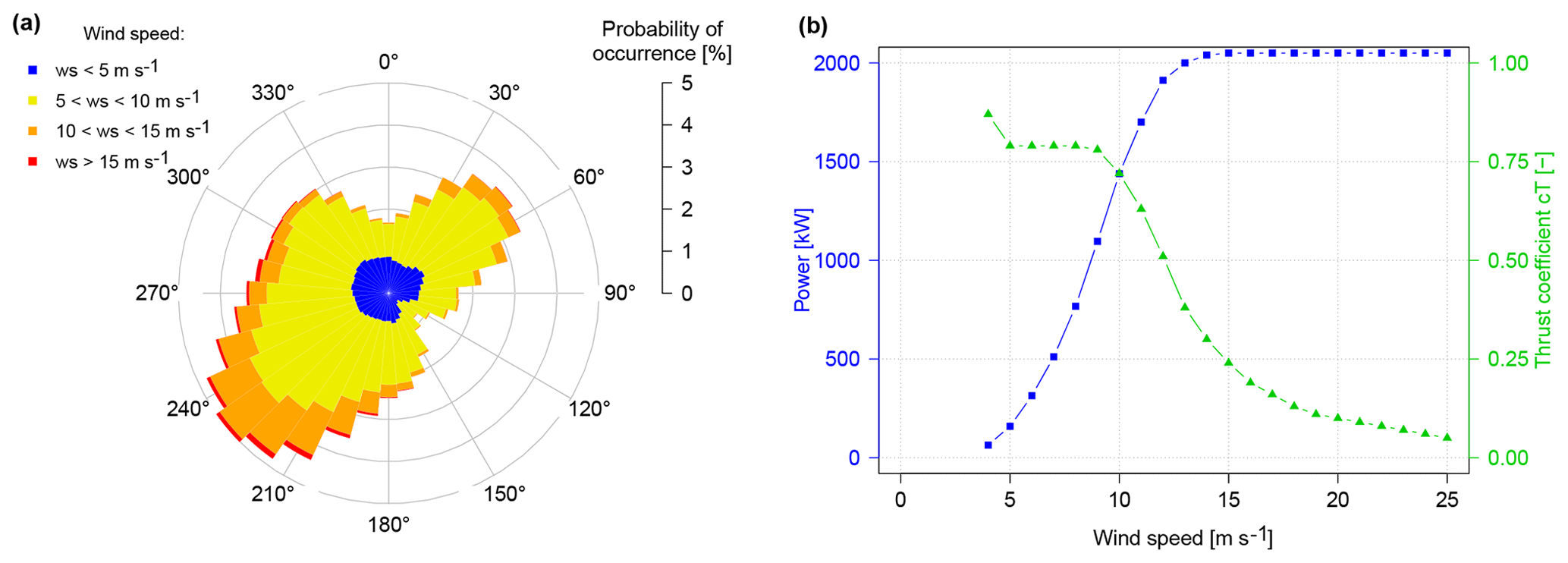
Figure 2Long-term wind rose observed at the site of the SMV wind farm (a) and Senvion MM82 guaranteed power and thrust coefficient (cT) curves (b).
It can be seen that wind turbines are more or less aligned on a north–south axis, while the prevailing wind direction is south-west, as seen on the long-term wind rose of Fig. 2a. This particular wind farm was chosen for the field test campaigns of the SMARTEOLE project because of the proximity with ENGIE Green maintenance centre (located 5 km away from the farm) and the wake events SMV6–SMV5. Indeed, due to development constraints, these two turbines were installed very close from each other (only 305 m, i.e. 3.7 D) and aligned with prevailing wind directions. In this paper, supervisory control and data acquisition (SCADA) data from the seven turbines are analysed along with data from a 80 m met mast and a ground-based lidar (Windcube V1). The location of these sensors is indicated in Fig. 1.
3.1 Original model
The Jensen model as it was originally developed by Jensen (1983) and Katic et al. (1986) is introduced briefly here. In this model, the wake grows linearly at a rate driven by a coefficient kw called wake decay constant (WDC) or wake expansion coefficient. The wind speed deficit δw in the wake is assumed to be uniform, axis-symmetric and depends only on the downstream distance x and the upstream wind turbine thrust coefficient cT. It can be computed using mass conservation and can be expressed as
where U0 is the incoming wind speed at the upstream wind turbine, Uw the velocity in the wake and R the radius of the upstream rotor.
When summing the wakes from two or more upwind rotors, wind speed deficits are aggregated via quadratic sum. Therefore, the wake deficit δn at the nth wind turbine of a row is simply given by
where δi is the wind speed deficit due to wind turbine i.
As indicated earlier, the Jensen model is probably the most widely used wake model for wind energy engineering applications, and that is mainly due to its simplicity and robustness. In particular, its very low computational cost makes it very suitable for optimization purposes, as a high number of simulations can be run in a very short time. However, although this model gives a fairly good estimation of the averaged power deficit in a wind farm (Göçmen et al., 2016), some studies underline its inaccuracy when it comes to looking at the individual power production of the wind turbines (Barthelmie et al., 2009; Gaumond et al., 2014). This is a crucial issue for power optimization using coordinated control, given that the production at the downstream turbines must be predicted as accurately as possible in order to choose the optimal settings of the upstream turbine.
There is therefore a need for improvement to be able to use this model for such purposes. Over the past years, some new models have been derived from the main equation of the Jensen model. They aim at offering a better representation of the individual wake deficits by introducing new parameters and equations, while keeping a low computational cost. For example, in Bastankhah and Porté-Agel (2014), the equation of momentum conservation is included to the model and a Gaussian distribution is assumed for the velocity deficit profile. The multizone model developed by Gebraad et al. (2014) is also Jensen based and considers three different areas in the wake, each with its own wake decay constant. Description of wind turbine wakes is indeed very much improved with these models; however, they can be relatively difficult to calibrate, as they consider up to 10 parameters that need to be tuned properly (Annoni et al., 2018).
In this paper, a very simple tuning of the original Jensen model is proposed based on the measure of local turbulence intensity (TI). The idea is to keep the simplicity of calibration and robustness of the model while improving its accuracy. As it will be discussed in the next section, and shown later in Sect. 4, taking turbulence intensity into account when tuning the model already significantly improves the performance of the model and offers a fairly good representation of the velocity deficit along a row of turbines, both onshore and offshore.
3.2 Tuning of the model
As can be seen in Eq. (1), there is only one parameter to be tuned in the Jensen model: the wake decay constant. This empirical constant is supposed to vary from one wind farm to another but generally the two recommended values of 0.075 and 0.05 are used for onshore and offshore wind farms, respectively (Mortensen et al., 2011). In some studies, it is also expressed more specifically as a function of the particular conditions at the wind farm, using, for example, the roughness length and the atmospheric stability (Peña and Rathmann, 2014) or the ambient turbulence intensity (Peña et al., 2015; Thorgersen et al., 2011). The link between wake growth and TI was pointed out by Lissaman (1976), but more recent studies, based on wind tunnel, large eddy simulations (LESs), Reynolds-averaged Navier–Stokes (RANS) simulations and full-scale turbine data, clearly identify TI as one of the most influencing parameters on the wake growth and magnitude of the wake deficits (Bastankhah and Porté-Agel, 2014; Mittelmeier et al., 2017; Santhanagopalan et al., 2018; Annoni et al., 2018).
It is known that TI varies significantly inside a wind farm, as the wake-added TI from upstream wind turbines is added to the ambient TI (Crespo et al., 1999; Vermeer et al., 2003; Göçmen and Giebel, 2016). Keeping the same wake decay constant for all wind turbines in the farm can therefore lead to errors in prediction of individual power production. The wake deficit is underestimated at the first few downstream turbines and overestimated further down the row (Gaumond et al., 2014), or vice versa (Göçmen et al., 2016). Consequently, it appears more accurate to assign a new wake decay constant for each wind turbine that would be directly linked to the local value of TI rather than considering an averaged value for the complete wind farm.
This strategy was followed in Niayifar and Porté-Agel (2016) and an expression between the wake decay constant and the local TI was proposed on the basis of LES data:
where (TI)mod is the modelled local TI obtained through the combination of ambient and wake-added TI, the latter being estimated thanks to the empirical equation developed by Crespo et al. (1996). As in this present paper SCADA data are available, it was rather decided to use the direct measurement of turbulence intensity provided at each wind turbine rather than relying on such a generic expression. In the next section, several methods are presented that can be used to estimate TI from SCADA. A direct proportionality is considered between kw and the measured TI, (TI)meas. This was done in order to keep the same simplicity as in the original Jensen model, i.e. to have only one parameter to calibrate, the constant c:
It should be noted that the tuning of the wake decay constant is based on TI only. Although TI is probably the most critical parameter, some studies underline the link between the variation of cT and kw (Bastankhah and Porté-Agel, 2014; Annoni et al., 2016). Accordingly, in Sect. 4, the tuning of the Jensen model is evaluated in the constant cT region (see Fig. 2) in order to isolate the local turbulence effects on the wake expansion. However, this is no longer true in Sect. 5, where the model is used in an optimization process involving axial induction control, whose purpose is precisely to change the cT of upstream turbines.
3.3 Estimating TI from SCADA
There are several ways to assess the incoming wind speed from ordinary SCADA signals, all with their advantages and drawbacks. These different methods are presented in this section and they can all be used to derive a local estimation of TI which is a required input for the wake model presented above. Alternative methods using sensors that are usually not installed on wind turbines (e.g. lidars or spinner anemometers) are not developed here but could also fulfill the same purpose.
The first and most obvious way to obtain a wind speed measurement from SCADA is to consider the nacelle wind speed signal (NWS) emitted by the nacelle anemometers installed on the wind turbine. However, these sensors are located behind the rotor and are therefore exposed to a highly distorted flow (Zahle and Sørensen, 2011). They cannot be relied on to provide an accurate and instantaneous wind speed measurement, but when it comes to considering local TI they might be good enough as only 10 min average and standard deviation values will be involved.
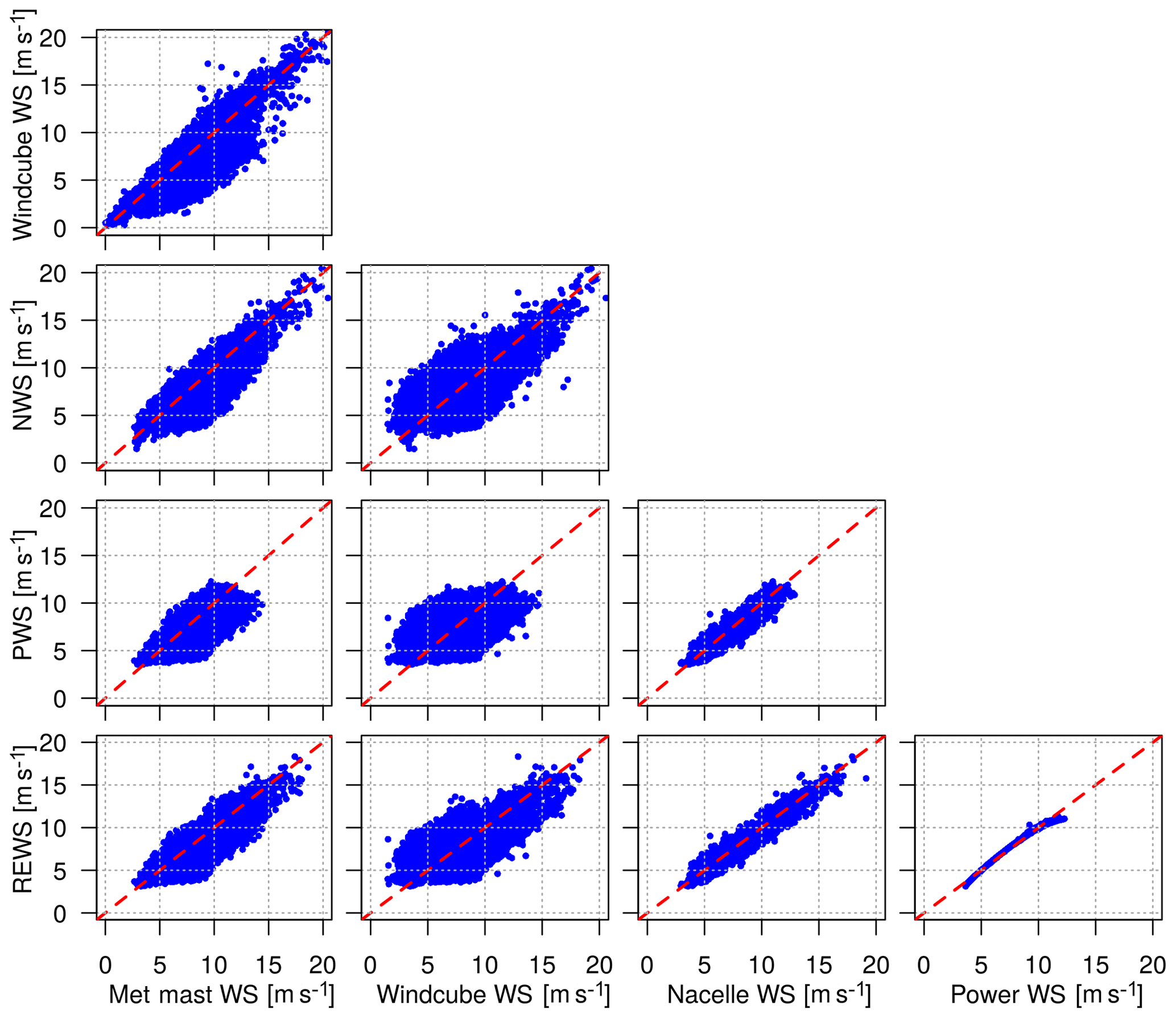
Figure 3Comparison of wind speed measurements at SMV5 (for nacelle wind speed, power wind speed and rotor effective wind speed) and at external sensors (met mast and Windcube). No sector filtering was applied to the data, explaining the scatter when comparing sensors at different locations.
Another wind speed measurement can easily be obtained from the active power production signal and the guaranteed power curve of the wind turbine (or a measured power curve). This new signal, labelled here as power curve wind speed (PWS), is generally more reliable than the NWS since the sensor is the wind turbine itself. Also, due to rotor inertia and the fact that the wind speed derived using this method is averaged over the whole rotor area, small fluctuations of the wind flow will be filtered out, resulting in a much smoother signal. The main issue regarding this method is its limited applicability: it cannot be used above rated wind speed or during down-regulation and therefore is unsuitable for wind farm coordinated control purposes.
In order to solve this problem, a third way was developed in the scope of the PossPOW project by Göçmen et al. (2014) to calculate the rotor effective wind speed (REWS) of a wind turbine in these particular situations. In this method, the REWS is calculated from three SCADA signals (active power, rotor speed and pitch angle) and a cP model. It must be ensured that the chosen cP model is fitting as best as possible to the real cP curve. Alternatively, a cP look-up table can also be used, when available. In this paper, the cP model and the value of its parameters are the same as those presented in Göçmen (2016), as they proved to offer a good performance for wind turbines in the same range (rated power of 2 MW with a diameter of about 80 m) as the ones studied here.
Overall, 4 months of 1 Hz SCADA data were processed (1 December 2015–31 March 2016) for the wind turbine SMV5 to compute 10 min average wind speed and turbulence intensity using these three different methods. Figure 3 compares these wind speed values with measurements from reference sensors (met mast and Windcube). No sector filtering was applied to the data; consequently, a significant scatter can be found when comparing two sensors at different locations due to wake effects. It can be observed that these results are very similar to the ones that were obtained at the Lillgrund offshore wind farm and were presented in Göçmen and Giebel (2016), showing a very nice correlation between the PWS and the REWS and more scatter when considering the NWS. This is because the wind speeds calculated through the REWS or PWS methods contain a geometrical averaging of the wind flow over the whole surface of the rotor which smooths out wind speed fluctuations (Göçmen and Giebel, 2016). On the other hand, NWS and met mast are point-wise measurements and therefore are affected by every single variation of the wind speed.

Figure 4Comparison of TI measurements at SMV5 (for nacelle wind speed, power wind speed and rotor effective wind speed) and at external sensors (met mast and Windcube), represented against wind direction. Error bars shows the 68 % normalized confidence interval (represented for NWS but a same order of magnitude can be expected for other sensors in the same wind direction bin). Vertical lines indicate position of wakes for SMV5 sensors and Windcube.
In Fig. 4, the turbulence intensity calculated from all these signals is represented against wind direction (5∘ bins). It can be seen that outside any wake events, the TI obtained through the NWS signal is of same order of magnitude than the one measured by external sensors. On the contrary, TI obtained with either the PWS or the REWS signals is approximately twice as low. As previously mentioned, this is explained by the geometrical averaging provided by these two methods.
All wake events are clearly captured by any of the TI signals. At a particular location of a wake, the TI measured is about twice as high compared to the free-stream conditions, indicating that wake-added TI is significant and can be measured reliably with a SCADA signal. Consequently, any of these TI signals could be used as input for the tuned wake model; it is simply needed to adjust accordingly the value of the constant c in Eq. (4). However, for the rest of this paper, only the NWS TI could be considered in practice, given that the PWS signal cannot be used for down-regulation purposes, while the REWS method requires acquisition and processing of second-wise data, which were not available for some of the turbines in the wind farm.

Figure 5Layout of Horns Rev-I offshore wind farm with turbine spacing and wind direction angle used in this study (a) and Vestas V80-2MW guaranteed power and thrust coefficient (cT) curves (b).
4.1 Data filtering and processing
The performance of the tuned Jensen model is now assessed in this section and compared to the results obtained for the original model. Production data from two wind farms are considered: the onshore SMV wind farm and the offshore wind farm of Horns Rev-I (layout of the farm and power and cT curves for the Vestas V80-2MW wind turbines are shown in Fig. 5). In both cases, the normalized power production along a row of turbines is analysed. The data are filtered to keep only the 10 min periods when all wind turbines are in operation and the incoming wind direction is within a ±5∘ interval around the main orientation of the row. Another filtering is done based on the power production of the most upstream turbine in order to consider only the 10 min periods when wind turbines are all in the constant cT region (region II of the power curve).
For each valid 10 min period, the power production deficit at each wind turbine is simulated for both the original and the tuned models. When considering the original Jensen model, the value of kw is calibrated using the first wake event of the row. In the case of the tuned wake decay constant, the value of the constant c in Eq. (4) is adjusted roughly to limit the individual error of the model along the row. The value used for (TI)meas is the 10 min TI measurement from the NWS signal. The normalized simulated deficits are then averaged over all valid 10 min periods and compared with the normalized measured deficits. The averaged value of the NWS TI signal at each wind turbine is also drawn to show the variation of the measured TI along the row of turbine. Error bars in Figs. 6 and 7 indicate the 68 % normalized confidence interval.
At SMV wind farm, the power production deficit is studied along row SMV1 to SMV5. The wind direction sector considered is 5 ± 5∘, and the valid power range for the most upwind wind turbine (SMV1) is fixed to 600–1100 kW to fulfill the constant cT condition. The filtered data set finally consists of 156 valid 10 min periods recorded between 15 June 2015 and 1 August 2016 (due to small occurrence of northerly winds, it was needed to consider a longer period than the actual field tests to gather enough valid data). The wake decay constant for the original Jensen model was kept as 0.075, the traditional value for onshore wind farm as it proved to show good performance for the first wake event of the row SMV1–SMV2.
At Horns Rev-I wind farm, the power production deficit is studied along row number 5, from HR5 to HR95 (see layout of the farm in Fig. 5a). The wind direction sector considered is 270 ± 5∘, and the valid power range for the most upwind wind turbine (HR5) is fixed to 0–1200 kW to fulfill the constant cT condition. The filtered data set finally consists of 270 10 min periods recorded between 16 February 2005 and 25 January 2006. The value for the wake decay constant of the original Jensen was fixed to 0.09, which is much bigger than the value of 0.05 traditionally used for offshore wind farms but much more consistent with the measured deficits. It was already found in other studies (e.g. Niayifar and Porté-Agel, 2016) that using a wake decay constant of 0.05 was clearly overestimating the power deficit for the wind farm of Horns Rev-I, as it gives narrower wake growth within the wind farm.
4.2 Results
The evaluation of the original and the tuned Jensen models on SMV and Horns Rev-I wind farms is presented in Figs. 6 and 7, respectively. In both cases, the normalized deficit is shown as a function of distance to the most upstream turbine, as well as the difference between the modelled and the observed deficits at each wind turbine for different values of wake decay coefficient.
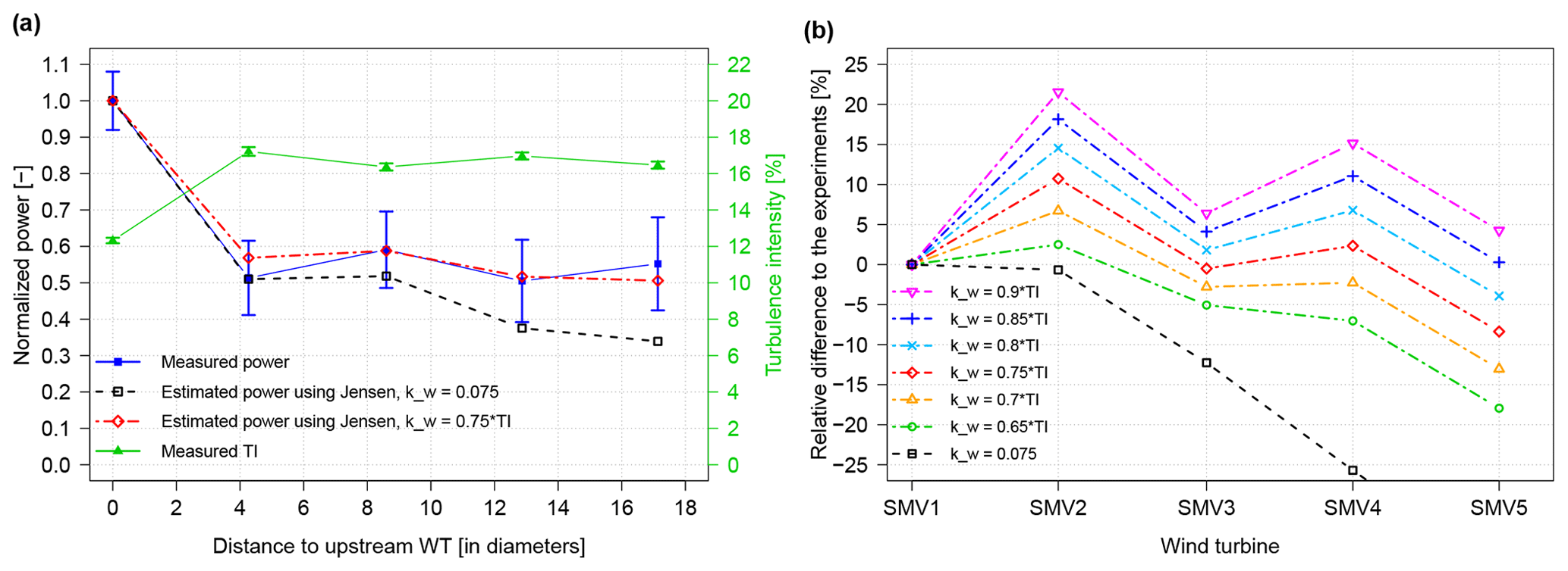
Figure 6Comparison of the model performance at SMV wind farm. Variation of experimental and modelled normalized power and turbulence intensity (measured by the nacelle anemometer) along the row (a) and variation of the error of the model at each wind turbine for various values of wake decay constants kw (b). Error bars indicates the 68 % normalized confidence interval.
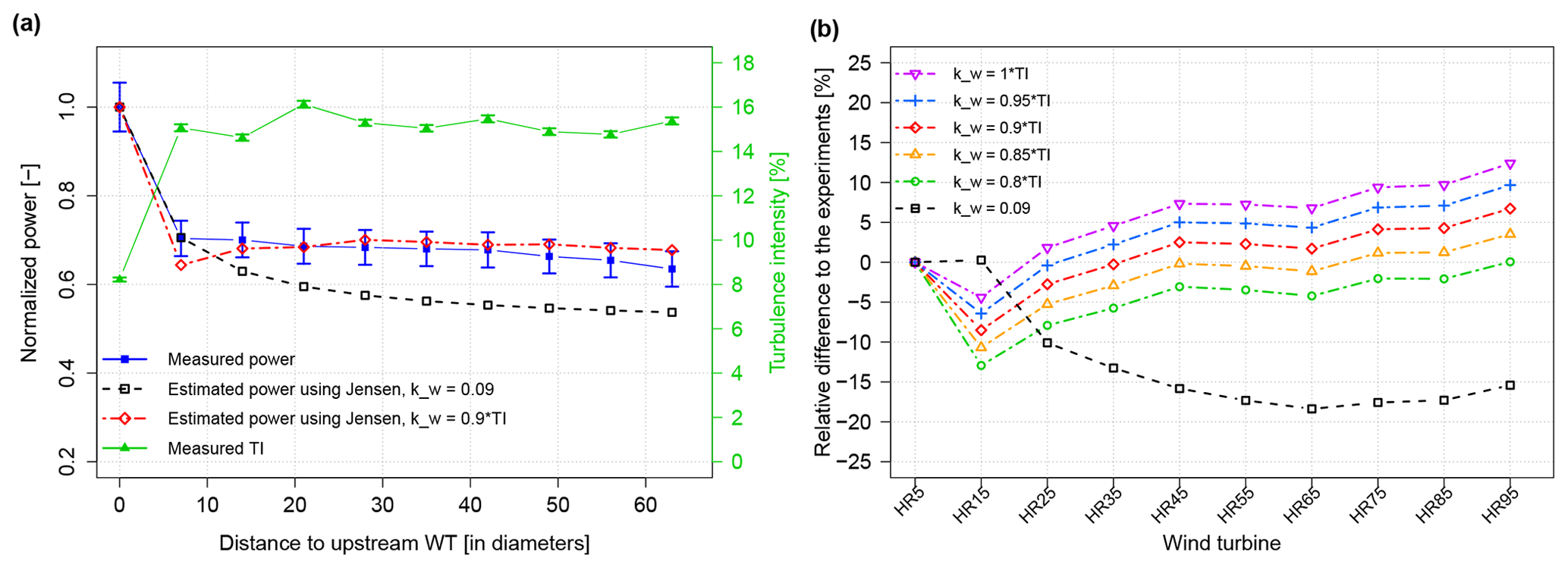
Figure 7Comparison of the model performance at Horns Rev-I wind farm. Variation of experimental and modelled normalized power and turbulence intensity (measured by the nacelle anemometer) along the row (a) and variation of the error of the model at each wind turbine for various values of wake decay constants kw (b). Error bars indicates the 68 % normalized confidence interval.
It can be seen that the graphs for the two wind farms have a very similar behavior, with the tuned Jensen model performing better than the original model. Except for the first wind turbine, the wake deficit calculated with the original model is always overestimated and the error becomes more significant towards the downstream direction: from approximately 10 % at the third turbine of the row, it goes around 15 % to 20 % further downstream. On the contrary, with the tuned Jensen model, the deficit is captured more accurately, especially at the wind turbines located in the middle of the row for which the error is kept at ±5 %. These changes are consistent with the augmentation of turbulence intensity from the second wind turbine in the row. Increased TI provides a better mixing between the disturbed flow in the wake and the undisturbed free flow, which allows a earlier recovery, both in terms of time and space. This particularity is taken into account in the tuned Jensen model since the WDC is increased linearly with TI, while the original Jensen keeping the same WDC all along the row leads to an overestimation of the deficit.
When analysing the impact of the choice of the constant c linking TI with the kw in the tuned Jensen model, two observations can be made. First, it can be seen that the optimal c obtained for each wind farm is different: 0.75 for SMV wind farm and 0.9 in the case of Horns Rev-I. This shows the sensitivity of the model to the local conditions and tends to indicate that a small calibration of the constant will still be needed for each wind farm to make sure that the wake deficit is correctly modelled. This site dependency of the Jensen model was already present in its original form; indeed, in this example, it can be seen that the best WDC obtained for the offshore wind farm (0.09) is much higher than the recommended values (0.04–0.05) and the one of the onshore wind farm (0.075).
The second observation is that the modelled wake deficit is varying regularly when c changes. This ensures that the calibration is as easy and robust as before, since it is simply needed to tune the value of c until the wake deficit is described as best as possible. Contrary to the original model, the accuracy is improved as taking into account the local TI allows a better representation of the individual wake deficit at each wind turbine.
Consequently, it can be concluded that this tuned Jensen model is providing an improvement compared with the original model, while keeping the simplicity of calibration and robustness of the original model. It can thus be used to define control instructions, as developed in the next section.
After having validated the performance of the tuned Jensen model, it is used in an optimization process to find the wind turbine settings maximizing their power performance. Only the axial induction strategy is developed here, due to its ease of application on a commercial wind turbine. Indeed, it simply requires to trigger a pre-implemented down-regulated power curve as a function of incoming wind conditions without modifying the control settings of the turbine. In practice, only wind speed and direction can be used as input for triggering a curtailment mode; therefore, power production is optimized for various wind speed and direction bins.
The hypotheses used during the optimization process are first presented, and then two study cases at SMV wind farm are analysed. Finally, a study of the uncertainty of the model outputs is realized based on the data from Horns-Rev I, and the values obtained are compared with the predicted gains.
5.1 cT estimation procedure
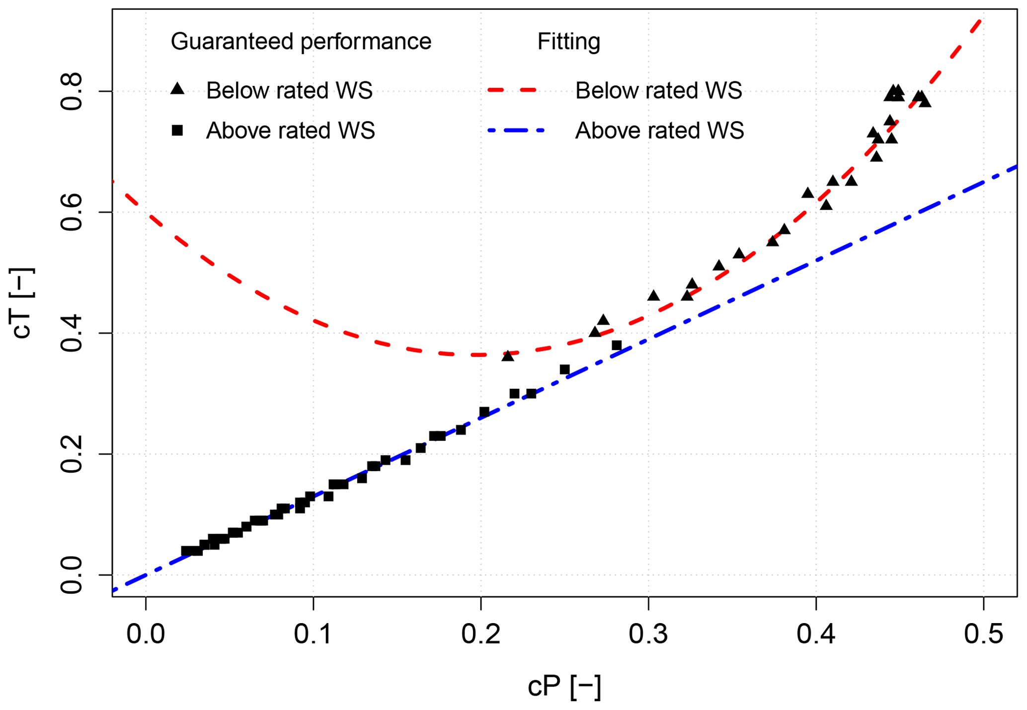
Figure 8Correlation between cP and cT for a Senvion MM82 wind turbine, deduced from the analysis of guaranteed power curve modes for sound management.
The principle of wind farm power optimization using an axial induction control strategy is to curtail the upstream wind turbines to gain more energy on downstream wind turbines. It is hoped that the decrease in the upstream cT will be high enough to reduce sufficiently the wake deficit so that the increase in production downstream can compensate for the upstream cP diminution. Consequently, it is a crucial issue to assess as accurately as possible how both cP and cT are being affected by the upstream down-regulation, in order to correctly estimate the overall production for various curtailment modes.
It is sometimes possible to use look-up tables to link cP and cT with operational parameters of the wind turbine, such as rotor speed and pitch angle. However, for this work, no look-up tables were available, and therefore another method had to be developed. A workaround was finally found by the analysis of MM82 guaranteed curtailed power curves used for noise emission reductions. Indeed, when representing cT against cP, as in Fig. 8, two different behaviours are being observed: one below rated wind speed (parabolic relationship) and another above rated wind speed (linear dependency).
Thus, an empirical relationship could be derived from this analysis, by fitting a second-order polynomial to the first set of data points and a first-order polynomial for the second one. The final relationship between cP and cT used for the optimization process and valid for an MM82 wind turbine is represented in Eq. (5) below.
5.2 Turbulence intensity distribution
As developed in Sect. 3, knowing the turbulence intensity is of primary interest to properly assess the wake deficit. In Sect. 4, the TI was calculated in 10 min timescale resolution to compare the performance of the tuned wake model with the original one. Here, due to practical constraints, it is not possible to consider the real-time TI as an input parameter for triggering a curtailment mode. Instead, it was decided to express the local TI as a function of wind speed and direction by calculating a TI distribution in the farm. Consequently, a different WDC is chosen for each wind turbine and each wind speed and direction bin, so that local TI still has some influence in the optimization process.
This TI distribution was obtained by averaging the NWS signal of all wind turbines in the farm in 10∘ direction bins and 1 m s−1 wind speed bins. The dependency of incoming TI for each wind turbine is represented for a wind speed of 8 m s−1 on a turbulence intensity rose in Fig. 9, alongside with TI measured by the met mast that can be used for comparison.
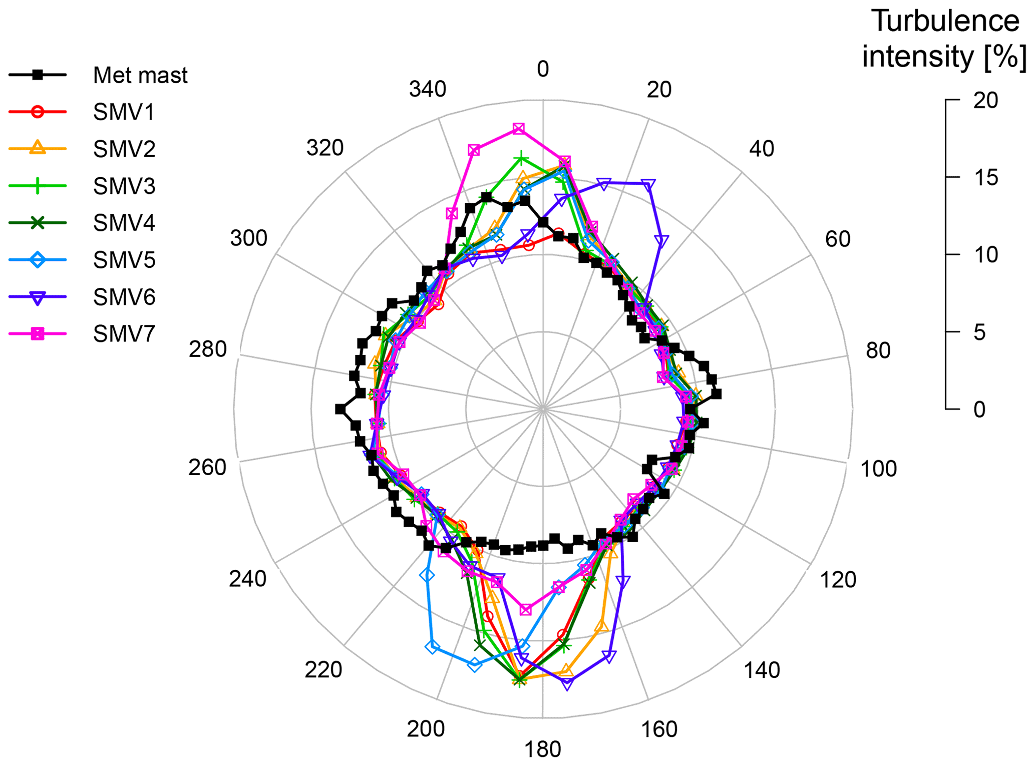
Figure 9TI distribution at each wind turbine used during the optimization process. This rose is obtained for a wind speed of 8 m s−1 only, but similar roses were calculated for each wind speed bin. Ambient TI measured at the met mast is also plotted for comparison.
It can be seen that the TI measured by the wind turbines outside any wake events is around 9 %–10 %, which is consistent with the met mast measurements. Some particular terrain effects can nonetheless be observed. Between 160 and 220∘, the TI measured by SMV7 is increasing up to 12 % to 13 %: this was attributed to the presence of a wood south of the farm and very close to SMV7 (please refer to the map of the wind farm in Fig. 1). Likewise, an increase of 1 % to 2 % in the SMV1 TI is observed for wind direction between 340 and 20∘. The reason for this increase was related the presence of the motorway at the north of the farm; indeed, the met mast curve shows also a similar increase in the sector [320∘; 0∘], corresponding to the direction of the motorway as seen by the met mast location.
5.3 Reduction of wake-added TI
In order to describe as accurately as possible the variation of TI in the farm when optimizing the power production, the influence of the upstream curtailment on downstream wake-added TI must be taken into account. Indeed, as the upstream wind turbine is down-regulated, the wake-added TI emitted by this turbine is reduced. It is expected that this decrease will be more and more significant as the upwind curtailment increases. Therefore, the TI distribution presented in the previous section, and calculated for normal operation conditions, is no longer valid: it must be reduced accordingly with the percentage of down-regulation applied on the upwind turbine. This is important especially when considering a row of three turbines (or more), since the deficit at the third turbine is calculated based on TI at the second turbine, which is itself dependent on the first turbine curtailment.
To study the impact of upstream down-regulation on downstream wake-added TI, data from the first field test campaign are considered. Between December 2015 and April 2016, SMV6 was occasionally curtailed of approximately 20 % for south-western winds (in the direction of alignment SMV6–SMV5). Analysing TI data provided by the nacelle anemometers, the wake-added TI, TIwa, can be computed with the following equation:
where TItot is the total TI in the wake measured at SMV5 and TIamb the ambient TI measured at SMV6.

Figure 10Variation of wake-added TI as a function of wind direction, in normal operation and during SMV6 curtailment. Error bars indicate the 68 % normalized confidence interval.
Table 1Comparison of measured wake-added TI at SMV5 wind turbine between no curtailment and 20 % curtailment on SMV6, with their 68 % normalized confidence interval. N/A (not applicable) indicates missing data for some wind direction bins.
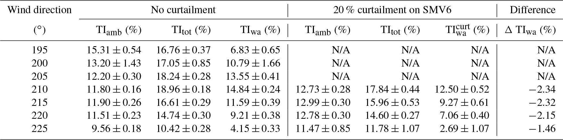
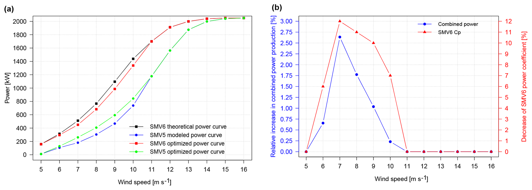
Figure 11Optimization of power production of SMV6 and SMV5. Power curves in the base and optimized cases (a) and variation of power gain and optimal SMV6 cP as a function of wind speed for the optimized case (b).
Ambient and total TI were binned against wind direction (5∘ bin width) and wake-added TI was deduced for each bin. Results are shown in Fig. 10, while numeric values are summarized in Table 1. Unfortunately, for the 20 % curtailment case, only data on the right side of the wake could be exploited. However, it still provides a very interesting insight of TI reduction with down-regulation as it covers full wake situation (at 210∘) to partial wake situations (220–225∘).
It can be observed that the upstream wind turbine curtailment provides a relatively significant decrease in downstream wake-added TI, as it is reduced from 14.84 % to 12.50 % for a wind direction of 210∘. As expected, as wind direction increases and we go from full wake situation to partial wake situation, reduction of wake-added TI becomes smaller, from 2.34 % to 1.46 %. In this paper, to model the relationship between percentage reduction of wake-added TI with percentage of upstream down-regulation, a linear dependency was assumed for a given wake condition:
The value of the parameter pwake linking ΔTIwa with %DR is expected to be dependent on the relative wind direction between the turbines. Consequently, the parameter for full wake conditions, pfw, will differ from the one for partial wake conditions, ppw. In this example, where a 20 % down-regulation was applied, values of (from the bin 210∘) and (from the bin 215∘) could be computed.
In Sect. 5.4.2, dealing with power optimization in a multiple wake case, reduction of wake-added TI with upstream curtailment is modelled with the following steps:
-
First, wake-added TI at each wind turbine in normal operation is calculated based on the TI distribution presented in Sect. 5.2 and ambient TI deduced from the most upstream wind turbine.
-
Second, as upstream wind turbines are being gradually curtailed in the optimization process, wake-added TI is adjusted based on Eq. (7) above. To simplify the process, only down-regulation of the closest upstream turbine is considered for the reduction of wake-added TI. A similar procedure was followed in Niayifar and Porté-Agel (2016) when modelling wake-added TI.
-
Finally, total expected TI at the wind turbine is calculated by inverting Eq. (6). This calculated TI can then be given as input into the local TI-based wake model to compute the wake deficit at downstream turbines.
5.4 Study cases
5.4.1 Wind turbines SMV5 and SMV6 (single wake case)
The first case to be studied is the SMV6–SMV5 wake event. It is of particular interest because of the very short spacing between the two wind turbines and their alignment close to prevailing wind directions. For this study case, a very simple optimization procedure is used: for each wind speed and relative wind direction, the cP of SMV6 is gradually decreased up to 20 % of its actual value (and the cT adjusted consequently based on Eq. 5) and the power production of both wind turbines is computed using the tuned Jensen model. The optimized power curve for SMV6 is then deduced from all the cP values giving the best combined production at each wind speed.
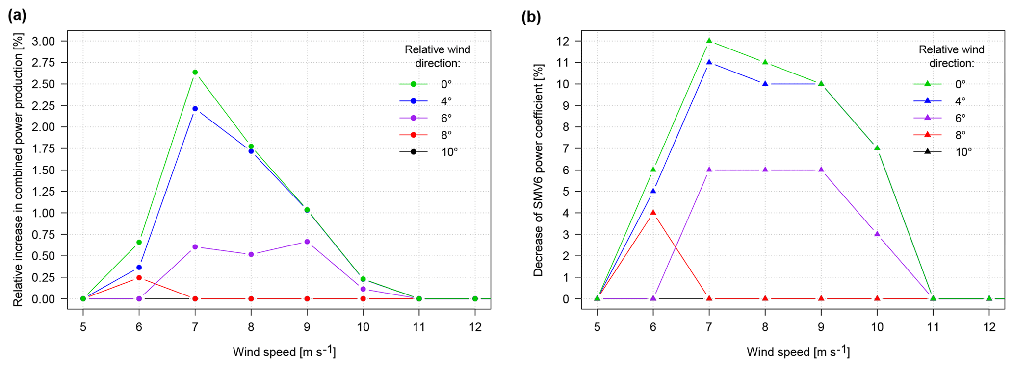
Figure 12Influence of changing relative wind direction. Variation of power gain (a) and optimal SMV6 cP (b) as a function of wind speed.
Results are presented in Fig. 11 for full wake conditions. In Fig. 11a, power curves for both wind turbines are plotted, while Fig. 11b shows the relative increase in combined power production which is obtained at each wind speed with the associated amount of curtailment which is applied to SMV6. It is observed that the maximum gain represents an increase of about 2.5 % and is found at 7 m s−1 when SMV6 is curtailed by 12 % (cP decreases from 0.46 to 0.405, while at the same time cT is reduced from 0.79 to 0.63 according to Eq. 5). More generally, it can be seen that the interest of coordinated control is limited to the wind speed range 5–11 m s−1, i.e. when both cP and cT of the upstream turbine are high. In this range, a small decrease in cP causes a high reduction of cT, as illustrated on the parabolic cP–cT relationship of Fig. 8. As wind speed increases further, the upstream wind turbine naturally starts to pitch to limit power production to its nominal value, and therefore axial induction control is no longer beneficial.
In Fig. 12, the impact of a changing relative wind direction on the relevance of applying a coordinated control is studied, showing the optimal gain that can be expected (Fig. 12a) and the optimal amount of curtailment required on SMV6 (Fig. 12b) as a function of the wind speed. It is seen that the wind direction sector on which gains can be observed is particularly narrow. As soon as the full wake condition is no longer respected, i.e. for relative wind direction above ±5∘, the benefit of axial induction control drops almost instantly: when wind direction shifts from 4 to 6∘ at 7 m s−1, gains are reduced from 2.25 % to approximately 0.6 %. This sensitivity confirms the very limited applicability of a curtailment strategy for power production optimization and the difficulty to implement it in a real case situation. As it is only beneficial on a 10∘ width wind direction sector centred around full wake conditions, very steady incoming wind conditions are required to make sure that gains in power production will actually be observed.
5.4.2 Rows SMV1 to SMV5 (multiple wake case)
The second case to be studied is the row SMV1 to SMV5. The power production along the row is now studied for full wake conditions and a wind speed of 8 m s−1, for which the coordinated control is expected to give the highest possible gain. Two different control strategies are being investigated: in the first one, only the most upstream turbine (SMV1) is being curtailed, while in the second one each wind turbine is optimally curtailed so that total power along the row is maximized. In the first case, the optimum is reached thanks to the same method as in previous section, while for the second case the following procedure (adapted from Heer et al., 2014) is used:
-
Start with no down-regulation applied on the wind turbines: %DRi=0 % for .
-
For wind turbine i, from upstream to downstream, find the value %DRi maximizing power production along the row and considering that all other %DRj≠i remain constant.
-
Repeat step 2 until all %DRi values stay constant.
Reduction of wake-added TI was considered as developed in Sect. 5.3. A value was used for all wake events in the row except for SMV2 → SMV3, which corresponds to a partial wake event (the alignment of these two turbines is found for a wind direction of −2∘). A value of (deduced from wind direction bin 215∘ in Table 1) was used instead.
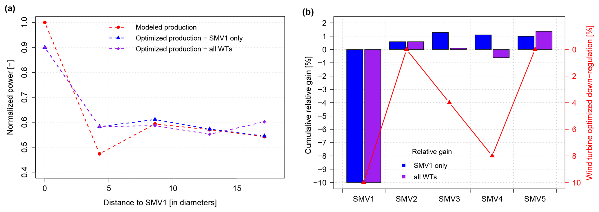
Figure 13Variation of normalized power at each wind turbine (a), cumulative relative gain and optimized down-regulation settings (b) along the row, for full wake conditions (wind direction of 5∘ at 8 m s−1).
Figure 13 shows the result of the process, with the normalized power production along the row (Fig. 13a) and the cumulative relative gain and the percentage of down-regulation at each wind turbine for the second strategy (Fig. 13b) (for the first strategy, the same amount of curtailment is applied to SMV1, while all other wind turbines are not curtailed). The cumulative relative gain allows following the change of power provided by the optimization as we move downstream, it is defined at wind turbine i as
Consequently, the cumulative relative gain at wind turbine SMV5 represents the total gain obtained thanks to the optimization process.
It can be seen from the figures that both strategies lead to an overall increase in power production, with the same amount of curtailment imposed on the most upstream turbine (10 % down-regulation). As seen on the cumulative relative gain which is positive at the second turbine, the increase in power at SMV2 is enough to compensate for SMV1 down-regulation. However, for the first strategy, as downstream wind turbines are not curtailed, most of the energy released by SMV1 is captured by SMV2 and SMV3 only. The most downstream turbines (SMV4 and SMV5) are only very slightly benefiting from the down-regulation and total relative increase is limited to approximately 1 %.
On the contrary, when following the second strategy, the energy made available by SMV1 down-regulation is more equitably shared between all downstream turbines. Indeed, SMV3 and SMV4 are also being curtailed so that high gains can be obtained for SMV5 (as SMV2 is not perfectly aligned with the rest of the row, it is not beneficial to curtail this turbine). As a consequence, the cumulative relative gain is decreased at SMV3 and SMV4, but when considering also SMV5 the total relative increase in power production is higher than in the first case, reaching almost 1.5 %. This confirms the idea that the best gains are obtained when each wind turbine is controlled individually to maximize the overall wind farm output and not their own power production.
5.5 Uncertainty quantification of the calibrated Jensen model
In order to put the optimized wind farm performance into perspective, it is essential to estimate the uncertainty of the model outputs. Since the calibration of the model is based on the operational turbine data, the uncertainty quantification (UQ) is established through the input uncertainty assessment and its propagation. The uncertainty is defined as the half width of the 68 % confidence interval, which corresponds to a distance of a single standard deviation.
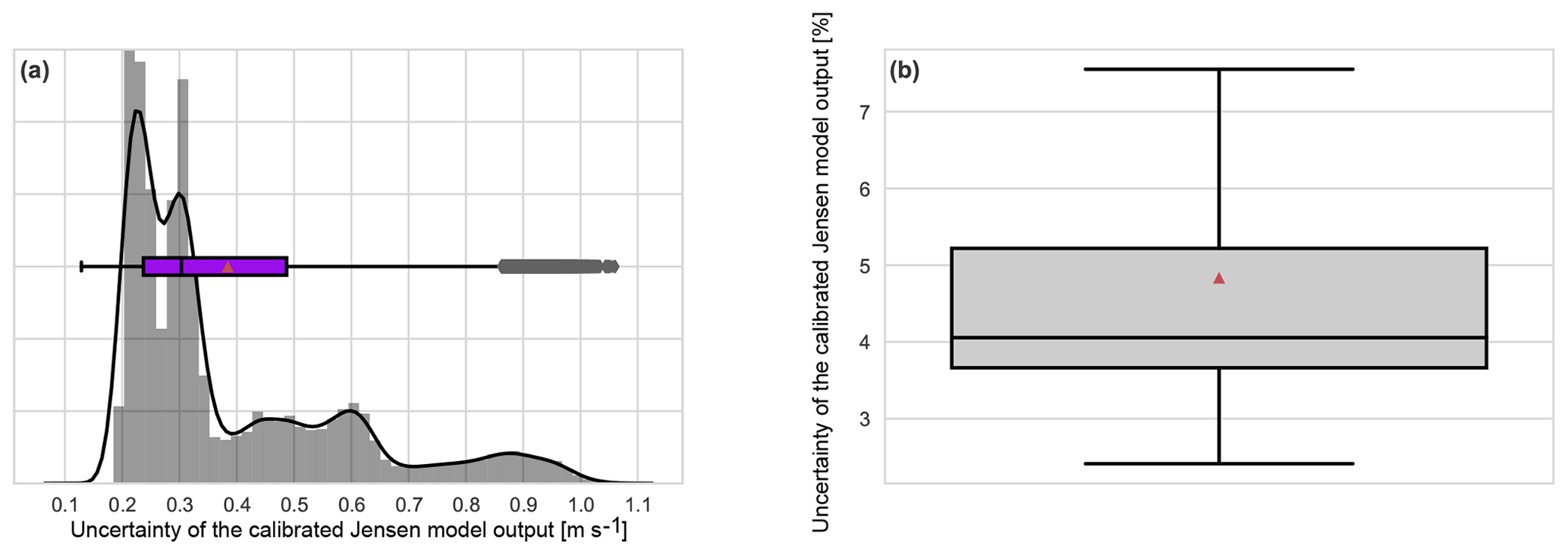
Figure 14Distribution of the uncertainty in the estimated wake velocity by calibrated Jensen model, (a) the histogram and the boxplot of the distribution in units (m s−1), (b) the boxplot of the percentage uncertainty distribution. The median, the boxes, the whiskers and the outliers are according to Tukey's descriptive statistics (Tukey, 1962). The red triangles indicate the mean.
In general terms, the uncertainties attached to the SCADA signals are indicated in the International Electrotechnical Commission (IEC) standards (IEC, 2013), where the main focus is the annual energy production estimates. With the same focus, Gaumond et al. (2012) investigated the wind direction uncertainty in particular, which is the most ambivalent input signal to the tuned Jensen model. Within 10 min intervals, the study showed the uncertainty to be at the levels of 5∘ for Horns Rev-I wind farm. However, since in this study the analysis is based on high-frequency data (second-wise data), the documented value of 3∘ uniform uncertainty in the yaw position signal (IEC, 2013) is considered for now. For the wind speed input, the dependency of the uncertainty to the operational range, i.e. regions II and III, is shown in Göçmen and Giebel (2018) for effective wind speed and in IEC (2013) for nacelle wind speed. Here, we consider the conservative estimate of 0.3 m s−1 with a Gaussian distribution, where the expected error is less with 90 % likelihood below the rated region. The uncertainty in wind speed is propagated through the estimation of TI (see Sect. 3.3), estimation of kw (see Eq. 4), estimation of cT and finally the estimation of wake deficit through Eq. 1. The resulting uncertainty distributions of the calibrated Jensen model are shown in Fig. 14. The uncertainty is propagated in a continuous time series of 18 h from Horns Rev-I wind farm, using a Monte Carlo analysis with 1000 realizations per second. The indicators in the boxplots follow Tukey's descriptive statistics (Tukey, 1962) where the boundaries of the whiskers are the lowest and the highest datum within the 1.5 interquartile range, IQR, corresponds to ±2.7σ from the mean.
Figure 14 shows that the uncertainty of the calibrated model output is not normally distributed. This is mainly due to the fact that along the propagation process, different sources and distributions of uncertainties are convoluted. It is also seen that there are many outliers in the distribution, which occur near the rated wind speed, i.e. around the operational transition between regions II and III as underlined in Göçmen and Giebel (2018). Along that transition region, the assessment of the cT is highly sensitive to the wind speed (see Fig. 5b), causing the propagation of the uncertainty to diverge. Since for the optimization scenarios discussed above the considered wind speed are lower, it is concluded that the conservative estimate of the model uncertainty can be stated as 0.3 m s−1 or, more generally, 4 %.
5.6 Towards field implementation
As already mentioned in the introduction of this paper, the optimized control strategies developed in these case studies are to be tested in a new field test campaign of the SMARTEOLE project. Through the comparison of the gains expected via these strategies in Sect. 5.4 and the uncertainty quantification of the previous section, it is very important to note that the tuned Jensen model risks not to provide the reported power increase in the field tests. In other words, the uncertainty of the model outputs and control inputs needs to be fully analysed in order to assess the true performance of the wind farm control approaches. Additionally, in order to see the full benefit of wind farm control schemes, more “accurate” sensors/data, more intelligent methods to analyse the data and different perspectives on how to include the physical complexity of the wind farm flow into the wake models are also needed.
Furthermore, the tuning of the model in the optimization process was focused to wind speed and direction only, as in practice these are the only two input variables that can easily be used for triggering the axial induction control for a wind farm operator having a limited access to the turbine control parameters. In reality, because of the highly fluctuating wind conditions (changes in wind speed, wind direction, turbulence intensity and atmospheric stability), a more complicated tuning would be required in order to decrease the risk of implementing innovative control strategies. Ideally, it would be more suitable to tune the WDC every 10 min (or at even shorter time periods) based on the latest measurement of wind speed, direction and local TI and then calculate in real time the optimized settings to be applied at each wind turbine. Since it would enable to include more dynamics and complexity of the local flow (both in terms of time and space), model adequacy would further improve and the resulting uncertainty would be reduced. However, this kind of scenario would also require much larger access to the wind turbine control parameters and goes beyond the scope of this present study.
Finally, it must also be mentioned that while the axial induction strategy seems to propose a limited benefit in terms of increased combined production compared to other strategies such as wake steering, its impact on wind turbine loads should be much more profitable. Indeed, thanks to the application of a curtailment on the upstream wind turbine, reduction in thrust and in the tower loads can be expected. Downstream, a decrease in the fatigue loading of the turbines can be predicted due to the reduction in the wake-added TI, as illustrated in Fig. 10 above. These results are interesting and highly relevant since load reduction can be related to an increased lifetime and therefore a decrease in overall cost of energy.
Field tests are currently being held on a commercial wind farm in France, Sole du Moulin Vieux, in the scope of a national project. The objectives of these tests are to study the potential of wind farm coordinated control strategies for power optimization and load reduction. In this paper, data from the first campaign were analysed in detail to propose a new tuning of the widely used Jensen model. This modification, based on the local measurement of turbulence intensity given by the nacelle anemometer, proved to be enough to improve the accuracy of the model and describe more precisely the individual wake deficit at each wind turbine. The simplicity of calibration and robustness of the original model is kept since there is still only one parameter to calibrate. This new tuning strategy was validated with data from SMV wind farm but also with data from a row of turbines at Horns Rev-I offshore wind farm.
Using this methodology, power production was optimized in two study cases at SMV wind farm. An axial induction strategy was considered with a model predictive approach, and a cT estimation procedure was developed in order to assess as accurately as possible the combined evolution of cP and cT during down-regulation of the wind turbines. Results from the optimization process show that a gain of 1 % to 2 % in aggregated power production can be expected for full wake conditions and wind speed between 7 and 9 m s−1. As wind direction changes or wind speed increases further, gains in power production obtained through the upstream wind turbine down-regulation quickly drop to zero, underlining the limited applicability of an axial induction strategy for power production optimization. Moreover, these gains have to be taken cautiously since some studies have already underlined discrepancies between model predictions and actual power productions of wind turbines, especially when variation of the wake decay constant due to changes in cT was not taken into account (Annoni et al., 2016). These results are in line with the performed uncertainty assessment of the tuned Jensen model, where the uncertainty is shown to be more than the predicted power increase. This also indicates the importance of an extensive uncertainty quantification on the simplified flow models to correctly evaluate the resulting wind farm control strategies.
However, even if the model is not as accurate as it could be, it is hoped that it is still good enough to give indications about optimal settings where gains would possibly be found. Based on the results derived in this paper, a new field campaign was realized between December 2017 and February 2018, during which a curtailment mode was applied to wind turbine SMV6. Data are currently being processed to determine whether augmentation in combined power production could be achieved. Furthermore, data from strain gauges installed in the blades still have to be analysed to study the impact of axial induction control on wind turbine fatigue loads. Given the quantified uncertainty, even though no gains in power production are obtained, a reduction in loads can be expected.
Future work about wind farm coordinated control realized in the scope of the SMARTEOLE project will also include the analysis of the potential of the wake steering strategy and the study of the dynamics involved when a wind turbine is curtailed or yawed.
As the underlying research data were collected on commercial wind farms, they could not be made publicly available. Please contact the corresponding author if you have any questions regarding the data used in this paper.
This work was undertaken by TD as a Master's thesis project under the supervision of OC, NG, GG and TG. TD developed the tuning of the model, did the experimental data analysis and the optimization of wind farm production, and wrote the article. Preprocessing of Horns Rev-I data and uncertainty quantification of the model was realized by TG. All authors had a part in reviewing and editing the manuscript.
The authors declare that they have no conflict of interest.
The authors would like to thank all the engineers and technicians from the Engie Green O&M centre for their help in setting up the experimental field tests of the SMARTEOLE project.
This research has been supported by the Agence Nationale de la Recherche in the scope of the project SMARTEOLE (grant no. ANR-14-CE05-0034).
This paper was edited by Raúl Bayoán Cal and reviewed by two anonymous referees.
Ahmad, T., Coupiac, O., Petit, A., Guignard, S., Girard, N., Kazemtabrizi, B., and Matthews, P.: Field Implementation and Trial of Coordinated Control of Wind Farms, IEEE Transactions on Sustainable Energy, 1169–1176, https://doi.org/10.1109/TSTE.2017.2774508, 2017. a
Annoni, J., Gebraad, P. M., Scholbrock, A. K., Fleming, P. A., and Wingerden, J.-W. v.: Analysis of axial-induction-based wind plant control using an engineering and a high-order wind plant model, Wind Energy, 19, 1135–1150, 2016. a, b
Annoni, J., Fleming, P., Scholbrock, A., Roadman, J., Dana, S., Adcock, C., Porte-Agel, F., Raach, S., Haizmann, F., and Schlipf, D.: Analysis of control-oriented wake modeling tools using lidar field results, Wind Energ. Sci., 3, 819–831, https://doi.org/10.5194/wes-3-819-2018, 2018. a, b
Barthelmie, R. J., Hansen, K., Frandsen, S. T., Rathmann, O., Schepers, J., Schlez, W., Phillips, J., Rados, K., Zervos, A., Politis, E., and Chaviaropoulos, P. K.: Modelling and measuring flow and wind turbine wakes in large wind farms offshore, Wind Energy, 12, 431–444, 2009. a
Bastankhah, M. and Porté-Agel, F.: A new analytical model for wind-turbine wakes, Renew. Energ., 70, 116–123, https://doi.org/10.1016/j.renene.2014.01.002, 2014. a, b, c
Bossanyi, E. and Jorge, T.: Optimisation of wind plant sector management for energy and loads, 2016 European Control Conference (ECC),, 922–927, IEEE, 2016. a
Crespo, A., Herna, J., et al.: Turbulence characteristics in wind-turbine wakes, J. Wind Eng. Ind. Aerod., 61, 71–85, 1996. a
Crespo, A., Hernandez, J., and Frandsen, S.: Survey of modelling methods for wind turbine wakes and wind farms, Wind Energy, 2, 1–24, 1999. a
Duc, T.: Optimization of wind farm power production using innovative control strategies, Master's thesis, Technical University of Denmark, available at: http://orbit.dtu.dk/files/134465852/DUC_Thomas_Master_thesis_final.pdf (last access: 12 May 2019), 2017. a
Fleming, P., Annoni, J., Shah, J. J., Wang, L., Ananthan, S., Zhang, Z., Hutchings, K., Wang, P., Chen, W., and Chen, L.: Field test of wake steering at an offshore wind farm, Wind Energ. Sci., 2, 229–239, https://doi.org/10.5194/wes-2-229-2017, 2017. a
Gaumond, M., Réthoré, P.-E., Bechmann, A., Ott, S., Larsen, G. C., Diaz, A. P., and Hansen, K. S.: Benchmarking of wind turbine wake models in large offshore windfarms, in: The science of Making Torque from Wind, European Academy of Wind Energy (EAWE), 2012. a
Gaumond, M., Réthoré, P.-E., Ott, S., Pena, A., Bechmann, A., and Hansen, K. S.: Evaluation of the wind direction uncertainty and its impact on wake modeling at the Horns Rev offshore wind farm, Wind Energy, 17, 1169–1178, 2014. a, b
Gebraad, P., Thomas, J. J., Ning, A., Fleming, P., and Dykes, K.: Maximization of the annual energy production of wind power plants by optimization of layout and yaw-based wake control, Wind Energy, 20, 97–107, 2017. a
Gebraad, P. M., Teeuwisse, F., van Wingerden, J.-W., Fleming, P. A., Ruben, S. D., Marden, J. R., and Pao, L. Y.: A data-driven model for wind plant power optimization by yaw control, in: American Control Conference (ACC), 2014, IEEE, 3128–3134, 2014. a
Göçmen, T.: Possible Power Estimation of Down-Regulated Offshore Wind Power Plants, PhD thesis, Technical University of Denmark, 2016. a
Göçmen, T. and Giebel, G.: Estimation of turbulence intensity using rotor effective wind speed in Lillgrund and Horns Rev-I offshore wind farms, Renew. Energ., 99, 524–532, 2016. a, b, c
Göçmen, T. and Giebel, G.: Uncertainties and Wakes for Short-term Power Production of a Wind Farm, 2018 Wind Energy Symposium, Kissimmee, Florida, 8–12 January 2018, https://doi.org/10.2514/6.2018-0252, 2018. a, b
Göçmen, T., Giebel, G., Poulsen, N. K., and Mirzaei, M.: Wind speed estimation and parametrization of wake models for downregulated offshore wind farms within the scope of PossPOW project, J. Phys. Conf. Ser., 524, 012156, https://doi.org/10.1088/1742-6596/524/1/012156, 2014. a
Göçmen, T., Van der Laan, P., Réthoré, P.-E., Peña, A., Larsen, G., and Ott, S.: Wind turbine wake models developed at the technical university of Denmark: A review, Renewable and Sustainable Energy Reviews, 60, 752–769, 2016. a, b
Heer, F., Esfahani, P., Kamgarpour, M., and Lygeros, J.: Model based power optimisation of wind farms, in: 2014 European Control Conference (ECC), IEEE, 1145–1150, 2014. a
IEC: IEC 61400-12-2, wind turbines: part 12-2: Power performance of electricity producing wind turbines based on nacelle anemometry, Tech. rep., International Electrotechnical Commission, 2013. a, b, c
Jensen, N.: A note on wind generator interaction, Tech. Rep. Risø-M-2411, Risø National Laboratory, Roskilde, Denmark, 1983. a, b
Katic, I., Højstrup, J., and Jensen, N.: A simple model for cluster efficiency, in: European Wind Energy Association Conference and Exhibition, 407–410, 1986. a, b
Knudsen, T., Bak, T., and Svenstrup, M.: Survey of wind farm control-power and fatigue optimization, Wind Energy, 18, 1333–1351, 2015. a
Lissaman, P.: Energy Effectiveness of Arrays of Wind Energy Collection Systems, Progress Report from Aero Vironment Inc, Pasadena, California, 91107, 40 pp., 1976. a
Machielse, L., Barth, S., Bot, E., Hendriks, H., and Schepers, G.: Evaluation of “heat and flux” farm control, Tech. rep., Energy research Center of the Netherlands, 2007. a
Mittelmeier, N., Allin, J., Blodau, T., Trabucchi, D., Steinfeld, G., Rott, A., and Kühn, M.: An analysis of offshore wind farm SCADA measurements to identify key parameters influencing the magnitude of wake effects, Wind Energ. Sci., 2, 477–490, https://doi.org/10.5194/wes-2-477-2017, 2017. a
Mortensen, N., Heathfield, D., Rathmann, O., and Nielsen, M.: Wind atlas analysis and application program: WAsP 10 Help facility, Tech. rep., Roskilde: DTU Wind Energy, 2011. a
Niayifar, A. and Porté-Agel, F.: Analytical modeling of wind farms: A new approach for power prediction, Energies, 9, 741, 2016. a, b, c
Pao, L. and Johnson, K.: A tutorial on the dynamics and control of wind turbines and wind farms, in: American Control Conference, 2009, ACC'09, IEEE, 2076–2089, 2009. a
Peña, A. and Rathmann, O.: Atmospheric stability-dependent infinite wind-farm models and the wake-decay coefficient, Wind Energy, 17, 1269–1285, 2014. a
Peña, A., Réthoré, P.-E., and Laan, M.: On the application of the Jensen wake model using a turbulence-dependent wake decay coefficient: the Sexbierum case, Wind Energy, 19, 763–776, 2015. a
Sanderse, B.: Aerodynamics of wind turbine wakes – Literature review, Tech. rep., Energy research Center of the Netherlands, 2009. a
Santhanagopalan, V., Rotea, M., and Iungo, G.: Performance optimization of a wind turbine column for different incoming wind turbulence, Renew. Energ., 116, 232–243, 2018. a, b
Thorgersen, M., Sørensen, T., Nielsen, P., Grötzner, A., and Chun, S.: WindPRO/PARK: introduction to wind turbine wake modelling and wake generated turbulence, Tech. rep., EMD International A/S, Aalborg (Denmark), 2011. a
Tukey, J. W.: The Future of Data Analysis, The Annals of Mathematical Statistics, 33, 1–67, https://doi.org/10.1214/aoms/1177704711, 1962. a, b
Vermeer, L., Sørensen, J., and Crespo, A.: Wind turbine wake aerodynamics, Progress in aerospace sciences, Prog. Aerosp. Sci., 39, 467–510, 2003. a
Wagenaar, J., Machielse, L., and Schepers, J.: Controlling wind in ECN's scaled wind farm, Proc. Europe Premier Wind Energy Event, 685–694, 2012. a
Zahle, F. and Sørensen, N.: Characterization of the unsteady flow in the nacelle region of a modern wind turbine, Wind Energy, 14, 271–283, 2011. a