the Creative Commons Attribution 4.0 License.
the Creative Commons Attribution 4.0 License.
 | 07 Nov 2019
Wind turbine load dynamics in the context of turbulence intermittency
Carl Michael Schwarz
Sebastian Ehrich
Joachim Peinke
The importance of a high-order statistical feature of wind, which is neglected in common wind models, is investigated: non-Gaussian distributed wind velocity increments related to the intermittency of turbulence and their impact on wind turbine dynamics and fatigue loads are the focus. Gaussian and non-Gaussian synthetic wind fields obtained from a continuous-time random walk model are compared and fed to a common aero-servo-elastic model of a wind turbine employing blade element momentum (BEM) aerodynamics. It is discussed why and how the effect of the non-Gaussian increment statistics has to be isolated. This is achieved by assuring that both types feature equivalent probability density functions, spectral properties and coherence, which makes them indistinguishable based on wind characterizations of common design guidelines. Due to limitations in the wind field genesis, idealized spatial correlations are considered. Three examples with idealized; differently sized wind structures are presented. A comparison between the resulting wind turbine loads is made. For the largest wind structure sizes, differences in the fatigue loads between intermittent and Gaussian are observed. These are potentially relevant in a wind turbine certification context. Subsequently, the dependency of this intermittency effect on the field's spatial variation is discussed. Towards very small structured fields, the effect vanishes.
- Article
(2082 KB) - Full-text XML
- BibTeX
- EndNote


Exact representations of wind and its dynamics are essential to the planning and design of wind turbines. So-called “wind models” are utilized to describe the dynamic behaviour. Guidelines, such as the International Electrotechnical Commission (IEC) standard 61400-1 for wind turbines (International Electrotechnical Commission, 2005), feature, for example, the Kaimal (Kaimal et al., 1972) and Mann (Mann, 1994) models. In addition to these models, for the wind fluctuations, deterministic wind gusts are considered to account for extreme events, such as the so-called “50-year gust”. The need for these additional wind scenarios indicates the incompleteness of wind models. Due to the high complexity of wind, modelling efforts are often focused on specific features, while neglecting others, as they are assumed to be of minor importance. The aforementioned examples focus on representing the spectral properties of wind velocity components and their coherence. This approach is widely accepted and reproduces the targeted features of wind well.
A known feature of wind which is not considered in common models is related to the statistics of wind speed increments uτ(t). Mathematically, uτ(t) can easily be obtained from a given lag value τ and a wind time series u(t) as
A comprehensive introduction to the characterization of wind by these statistics has been given by Morales et al. (2012). In short, the increments uτ(t) can be understood intuitively as changes in wind speed and therefore as a simple indicator for gusts. In conclusion, their dynamics might be relevant in the context of wind turbine performance and loads.
For wind, it is well documented that uτ(t) behaves in a non-Gaussian manner (Böttcher et al., 2003; Vindel et al., 2008; Morales et al., 2012; Mücke et al., 2011). In this work, this non-Gaussianity is referred to as the “intermittency of turbulence”1. However, wind models are commonly based on spectral properties and imply Gaussian-behaved uτ(t) (see e.g. Powell and Connell, 1986; Mücke et al., 2011). As elaborated on by Böttcher et al. (2003), the assumption of Gaussian uτ(t) leads to false predictions, especially about extreme events: events predicted to occur only every 500 years by a Gaussian model are predicted to occur five times a day if non-Gaussianity is considered. Thus, the question arises of whether or not the omission of intermittency in the wind modelling process is a safe simplification. If intermittency would have a relevant impact on wind turbine loads, this concept should be considered for implementation into future wind models. This work aims to answer this question by comparing intermittent wind fields against purely Gaussian ones with respect to their influence on wind turbine dynamics and loads.
This paper is organized as follows. Other studies have been dedicated to this issue. They are discussed in Sect. 1.1. The specific contribution of this work is described in Sect. 1.2. Detailed aspects about the approach of this work, especially about the wind modelling, are given in Sect. 2. The results are presented and discussed in Sect. 3. Summarizing conclusions are given in Sect. 4.
1.1 Literature overview
The discussion of non-Gaussian increments in the context of wind energy has been started by Böttcher et al. (2001, 2003). Intermittency has also been observed in data obtained from field measurements (Böttcher et al., 2003; Morales et al., 2012; Vindel et al., 2008). Further efforts focusing on non-Gaussian power increment statistics of single wind turbines and entire wind parks have been made (Wächter et al., 2012; Milan et al., 2013; Hähne et al., 2018), which can be interpreted as a footprint of the statistics of interest. Milan et al. (2013) were able to fit a non-linear scaling model including the intermittent wind dynamics to the scaling behaviour of both the wind and power output data, relating both of these dynamics. Lately, Hähne et al. (2018) reported on the intermittent power statistics of wind energy. These studies can be seen as evidence that intermittent dynamics of the wind are present in the entire wind energy conversion process. Deeper insight into how the intermittent wind dynamics excite the turbine is not presented in these works.
In order to generate intermittent wind dynamics, a wind model has been developed by Kleinhans (2008). It relies on the concept of continuous-time random walks (CTRWs) introduced by Montroll and Weiss (1965) and has been applied in related studies presented in the following. It is further utilized in this work. Details are given in Sect. 2.
Pioneering work with respect to intermittency and wind turbine loads was conducted by Gontier et al. (2007). The authors tested two standard wind models (Kaimal et al., 1972; Mann, 1994) and the intermittent CTRW wind model (Kleinhans, 2008) (see Sect. 2.1.1) with respect to their impact on fatigue loading of different sensors. Blade element momentum (BEM)-theory-based wind turbine computations were conducted. The authors drew conclusions to relevant load sensors, e.g. blade root bending moments and the tilt moment at the tower top. Differences in the fatigue loads for the different models were detected and described but could not be embedded into a clear overall trend. Although the direct comparison of different wind models is interesting, these models feature fundamental differences that will affect the wind turbine loads, e.g. spectral properties. In other words, intermittency is not isolated as the main difference between these wind fields. This represents an obstacle in drawing further conclusions from the presented study, as the reason for the deviations in the results obtained for different wind fields could also be a consequence of other statistical differences.
Mücke et al. (2011) adopted aspects of the methodology applied by Gontier et al. and added a comparison against measured wind data. Three types of wind field data were used: a measured data set from the GROWIAN site (Körber et al., 1988), a common Kaimal model (Kaimal et al., 1972; International Electrotechnical Commission, 2005) and the CTRW model (Kleinhans, 2008). All types of wind fields were processed with a purely aerodynamic BEM-based wind turbine model. The CTRW fields were designed in order to have similar increment statistics as the GROWIAN fields. For all types of fields, a high correlation between the wind increment statistics and the resulting torque increment statistics was reported. The authors showed that non-Gaussian wind statistics can lead to non-Gaussian torque statistics. A rain-flow-counting (RFC) analysis (Matsuishi and Endo, 1968) was conducted on the resulting torque data of the GROWIAN measurement field and the Kaimal field. It is concluded that the RFC method is not sensitive to the intermittent dynamics, as a certain amount of temporal information is lost within a RFC procedure. However, revisiting the results by Mücke et al. (2011), differences in the load range histogram especially at higher load ranges are evident which, when potentiated with the SN-slope coefficient2, could lead to pronounced differences in the equivalent fatigue loads (EFLs). Therefore, the conclusion that common fatigue estimation procedures, such as the RFC, are insensitive to intermittency is arguable. Mücke et al. (2011) add the comparison against measured wind data to the discussion, which is of high interest but also challenging: measured wind data commonly contain non-stationarities and trends, while wind models usually yield stationary time series.
A different approach to obtain intermittent wind fields was utilized in the study presented by Berg et al. (2016). The authors investigate wind fields derived from large-eddy simulations (LESs) of the atmospheric boundary layer (ABL). Snapshots of “frozen” three-dimensional velocity fields, exhibiting the intermittent dynamics, were extracted from the simulation result. The three spatial dimensions are converted into an unsteady two-dimensional velocity plane via Taylor's hypothesis of frozen turbulence and processed through a common aero-servo-elastic model of a wind turbine. Gaussian fields were obtained by deriving surrogate fields based on proper orthogonal decomposition (POD) of the original data. In doing so, the exact same second-order statistics were obtained for the surrogate, non-intermittent fields. Overall, 20 fields of each type were processed through a BEM-based aeroelastic wind turbine model in order to evaluate the impact of intermittency on wind turbine loads. Both ultimate and fatigue loads resulting from these simulations were compared. Based on an RFC-based fatigue analysis and an analysis of global load extrema, the authors do not find any significant evidence that intermittency alters the loads and therefore conclude that the relevant dynamics are low-pass filtered by the turbine, as they are mainly found in small structures below the rotor scale. The work by Berg et al. (2016) successfully delivers an approach that respects other statistics of wind fields and aims at the isolation of intermittency: the approach of generating a pair of wind fields with the same statistical properties – aside from the distribution of two-point statistics – is the preferable approach to analyse the impact of intermittency on wind turbine loads. This work follows this approach.
Schottler et al. (2017) compared Gaussian and non-Gaussian wind fields in an experimental campaign featuring a model wind turbine. The turbulent fluctuations in the experiment were achieved with an active grid. The authors compare the response of the model wind turbine to two different kinds of inflows: one with Gaussian, the other with non-Gaussian increment statistics. Both inflows are equivalent with respect to their standard deviation and mean value. The authors demonstrate that the turbine's response (e.g. the rotor thrust) still contains the non-Gaussian dynamics, contradicting the conclusion by Berg et al. (2016) that these dynamics are filtered by the turbine. However, Schottler et al. (2017) do not report on the size of the wind structures in the tested wind fields, which is related to the argumentation (Berg et al., 2016) and is also in the focus of this work. Secondly, only a few statistical wind parameters, which hamper the isolation of intermittency (see Sect. 2.1.2) and the ability to draw conclusions with respect to intermittency, could be controlled and made comparable.
In a recent national project (Thomas et al., 2017), the effect of intermittent wind dynamics on fatigue loads was tested. Synthetic (Kaimal et al., 1972; Mann, 1994) and intermittent CTRW fields (Kleinhans, 2008) were processed in a BEM-based wind turbine model. Subsequently, the resulting load time series were used as an excitation signal in an experimental setup, in which material probes were dynamically loaded until failure. Significant differences were observed, indicating much faster damage accumulation for intermittent wind. However, due to differences in the fields with respect to their spectral properties and coherence, these findings cannot be attributed to the non-Gaussian increment statistics exclusively. The application of intermittent dynamics to material probes, however, is highly interesting, as one does not rely on fatigue estimation procedures, as the sensitivity of these procedures to intermittent dynamics is in question.
In summary, contradicting conclusions with respect to the effect of intermittency on wind turbines have been drawn. It is still unclear how to judge the impact of these statistics, as some questions are still left open. Also, there is a need to discuss the proper isolation of intermittency within this issue.
1.2 Contribution of this work
This work aims to isolate and investigate the effect of non-Gaussian wind velocity increments on wind turbine systems compared to Gaussian ones. The key aspects added to the ongoing scientific discussion are as follows:
-
Firstly, we emphasize the importance of isolating intermittency and discuss the requirements that wind fields must fulfil in the context of this problem.
-
Secondly, this work shows that an intermittency effect is evident for spatially homogeneous wind fields based on aero-servo-elastic wind turbine simulations. Preliminary results were reported in Schwarz et al. (2018).
-
Lastly, this work contributes to the discussion by pointing out the critical importance of the size of coherent structures and the general concept of coherence to this problem.
To investigate the effect of intermittent vs. Gaussian wind, two synthetically generated wind field types are evaluated by means of wind turbine simulations and a subsequent load analysis. In the following, a comprehensive description into these synthetic wind fields is given in Sect. 2.1. The wind turbine model and the load analysis are discussed briefly in Sect. 2.2 and 2.3, respectively.
2.1 Wind fields
A central point of this work is the isolation of the intermittency effect. Hence, we searched for a method to generate wind fields with and without intermittency. Aside from intermittency, these fields have the same features. They are equivalent according to the wind field characterization of the IEC standard. This is achieved by the utilization of the CTRW model proposed by Kleinhans (Kleinhans, 2008), which is presented in detail in Sect. 2.1.1.
The resulting temporal dynamics are discussed in detail in Sect. 2.1.2 alongside the requirements for the isolation of intermittency.
The isolation of intermittency could only be assured for individual post-processed CTRW time series u(t), not for entire wind fields u(y, z, t) as demanded in common wind turbine simulations. In order to compose entire wind fields from those time series, simplified spatial correlations in the yz plane (parallel to the rotor disc) are considered. These are presented in Sect. 2.1.3.
General technical aspects about the wind fields are discussed in the following. Commonly, 10 min wind samples are considered, as the mean wind speed is assumed to be approximately stationary over this time span. Due to the high demand for data, in order for the presented dynamics to be resolved reasonably well, stationary time series of the length of 1 h are considered in this study. For each type of field, 10 realizations have been generated for each wind speed tested in this study. In order to investigate the impact on a model wind turbine profoundly, multiple mean wind speeds within the operation range of the turbine have been tested. These are 6, 9, 12.5, 15, 18, 22.5 and 25 m s−1. In order to obtain results independent from turbulence intensity (TI), TI is 10 % in all cases. The sampling frequency of each data set is fs=20 Hz. We assume the most relevant timescales of wind dynamics to the wind turbine system to be captured with this sampling frequency. As a consequence, the smallest increment lag value within this study is s. In the yz plane, a spatial discretionary of 31×31 equidistant grid points is used, spanning an area of 135 m × 135 m covering the rotor area. This results in a mesh size of dy = dz=4.5 m, which is approximately the size of a discretized blade segment dr in the utilized wind turbine model. For the sake of simplicity, the fields are uniform, meaning they do not consider shear, veer or similar aspects.
2.1.1 CTRW model
The model proposed by Kleinhans et al. (2008); Kleinhans (2008) is used for wind time series generation. It has been applied in previous studies related to the presented issue (Gontier et al., 2007; Mücke et al., 2011; Schwarz et al., 2018). Details are given in Appendix A. The models' main building blocks are two coupled Ornstein–Uhlenbeck (OU) processes and a stochastic mapping process, which are discussed in the following.
Velocity signals u(s) are generated as coupled OU processes (see Kleinhans et al., 2008) on a model-intrinsic timescale s. The resulting signal u(s) is a stationary Gaussian process. The utilization and implementation of OU processes is widely known and thus not discussed further here (see Appendix A).
The key feature of the model is the stochastic time-mapping process, which allows for the generation of intermittent dynamics. A mapping of the intrinsic timescale s to the physical timescale s→t is realized as
The mapping process τα,C is essentially a waiting time distribution. This idea is based on the concept of CTRWs (see e.g. Kutner and Jaume, 2017). Kleinhans (2008) proposes a stochastic Lévy process for τα. For , τα yields Lévy distributed random numbers larger than zero. In the case of α=1, the mapping is linear τ1=1, so that s=t and in return u(s)=u(t). In order to avoid waiting times τα→∞, the Lévy process is bounded to yield a maximum waiting time C.
The intermittency of u(t) is mainly determined by α and C. In this work, C=350 s and αint=0.65 are used for all intermittent cases. As mentioned above, αGau=1 for Gaussian cases. A complete parameterization is given in Appendix A.
2.1.2 Velocity time series for an isolated intermittency effect
The focus of this work is to assess the effect of different wind velocity increment statistics on wind turbine dynamics. For this purpose, wind time series with Gaussian and non-Gaussian (intermittent) increment statistics are generated and compared.
In order to investigate the impact of the increment statistics exclusively, one must isolate them: the wind time series need to be highly comparable with respect to other, lower-order statistics. For example, differences between two time series with respect to the resulting wind turbine fatigue cannot be attributed strictly to the intermittency effect if both time series differ not only in their increment statistics but also in other statistical quantities, say their standard deviations. To provide some reference, it was tested how sensitive the presented case is to changes in turbulence intensity. As a coarse overall trend, it was found that a 1 % gain led to a 1 % increased fatigue load for the load sensors discussed in this study. This relationship is highly dependent on the actual turbine, the load sensor, other wind field, etc., wherefore we do not claim this to be generally true.
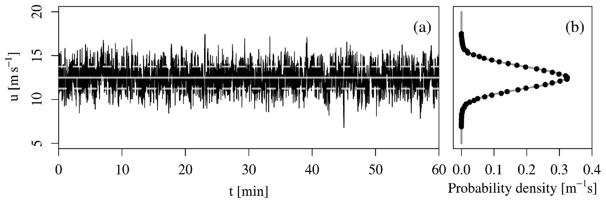
Figure 1Exemplary Gaussian wind time series. (a) Main wind velocity component u(t), including mean ± 1 standard deviation (dashed lines). (b) Corresponding histogram and Gaussian fit.

Both resulting types of time series feature the same mean values and variances. Also, the probability density functions (PDFs) of the velocity fluctuations are equivalent. These qualify as one-point (1P) statistical properties. All moments of the 1P statistics will be equivalent for both types of fields. In addition, the power spectrum which is related to the autocorrelation function via the Wiener–Khinchin theorem is assured to be comparable. These statistics are two-point (2P) statistics (alias increment statistics), more precisely 2P statistics of second order. The differences between both types of time series due to intermittency are evident in the fourth moment (and higher) of their 2P statistics. From turbulence theory, it is known that the third moment of increments should also be differing between intermittent and Gaussian fields, as it is linked to the four-fifths law of Kolmogorov (1941) (K41). This effect is not captured in our two types of time series, as both of them feature non-skewed increment distributions. However, for the impact on loading, we believe that the fourth moment is of much higher interest than the third moment. The third moment essentially determines the balance (or imbalance) between positive and negative wind speed increments. On the other side, the fourth moment similarly describes the balance (or imbalance) between large and small absolute amplitudes of the velocity increments. The amplitudes of wind speed increments are likely to correlate to some degree with the amplitudes of load cycles of a given load sensor. Therefore, we focus on the fourth moment of the increment statistics.
In the following, features of the resulting time series are presented in detail.
First, the 1P statistics are discussed. In order for the operation point of the wind turbine to be comparable, the mean wind speeds have to be the same. The strength of wind fluctuations is scaled by the turbulence intensity, which is the wind’s variance divided by the average wind velocity. Therefore, these have to be equivalent as well. Examples of time series for the main flow component u(t) are given in Fig. 1a for the Gaussian type and Fig. 2a for the intermittent type, respectively. It is evident that the mean wind speed and TI are equivalent between both types.
Furthermore, as shown in Figs. 1b and 2b, we achieve Gaussian velocity fluctuations u′(t) for both types. It was assured that the first four central moments of the 1P statistics do not deviate from their desired values by more than 10−3. We are thus convinced that 1P PDF and 1P moments are comparable. We like to stress that within a study like this one, a high comparability of 1P statistics must be assured before any observation in the results can be related to 2P statistics.

Figure 3Correlation coefficient ρ over lag value τ for 10 Gaussian and 10 intermittent realizations.
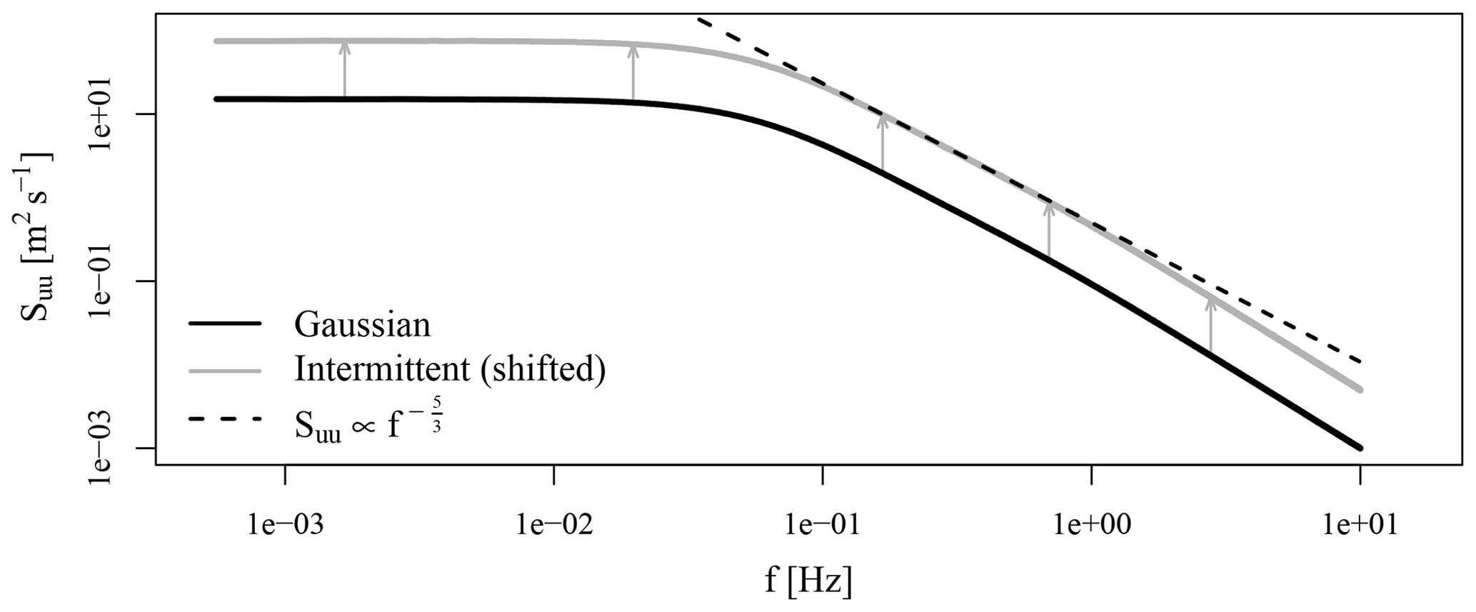
Figure 4Power spectral density (PSD) Suu for the main wind velocity component u(t) for the Gaussian and intermittent field types. Note that the intermittent spectra are shifted by a factor of 5 for better representation. The length of the arrows corresponds to the distance of the shift. The dashed line represents a slope relevant to K41.
Next, the 2P statistics of the generated time series are discussed. A common 2P statistic is the autocorrelation function:
It reflects how far wind structures extend in the longitudinal (in this case, the temporal) dimension. Figure 3 shows ρ(τ) for all intermittent and all Gaussian realizations. Aside from some scattering in the weakly correlated regime, a high agreement among all realizations is evident: the velocity dynamics are correlated for roughly 12 s, which in comparison to atmospheric turbulence is very short. This can presumably be explained by the lack of low-frequency dynamics in the velocity signal. It is evident from Figs. 1a and 2a that not too much low-frequency dynamics are present in our signals. The lack of those might potentially affect the presented results quantitatively but not qualitatively, as the differences in the presented results stem from the intermittency. We were unable to incorporate lower-frequency dynamics into the velocity signal within our CTRW approach, as our attempts spoiled other properties of our time signals. However, it is important to keep in mind that it is our highest priority to work with highly comparable Gaussian vs. non-Gaussian fields. This compromised some of the other wind field parameters.
As mentioned above, ρ(τ) is related to the power spectrum via the Wiener–Khinchin theorem. The power spectrum is commonly used to describe wind dynamics and has a known impact on the load dynamics (International Electrotechnical Commission, 2005; Veers, 1988). Figure 4 shows the spectral properties of u′(t) for both types of fields. Note that the intermittent spectrum has been shifted vertically for the sake of better representation. As expected from the autocorrelations, both types are described by highly comparable spectra. Also, within the frequency range 10, the spectra roughly follow a five-thirds trend, as postulated by Kolmogorov in 1941 (K41) (Kolmogorov, 1941).
The spectral and cross-spectral properties of the lateral and vertical velocity components are not discussed in this work. They have been modelled simply as white noise signals, wherefore statistically significant differences between Gaussian and non-Gaussian fields are expected to arise from these velocity components. In general, these velocity components can drive fatigue loads for some sensors and turbine components. However, in this work, we focus on the impact of longitudinal wind dynamics and only discuss a limited set of load sensors.
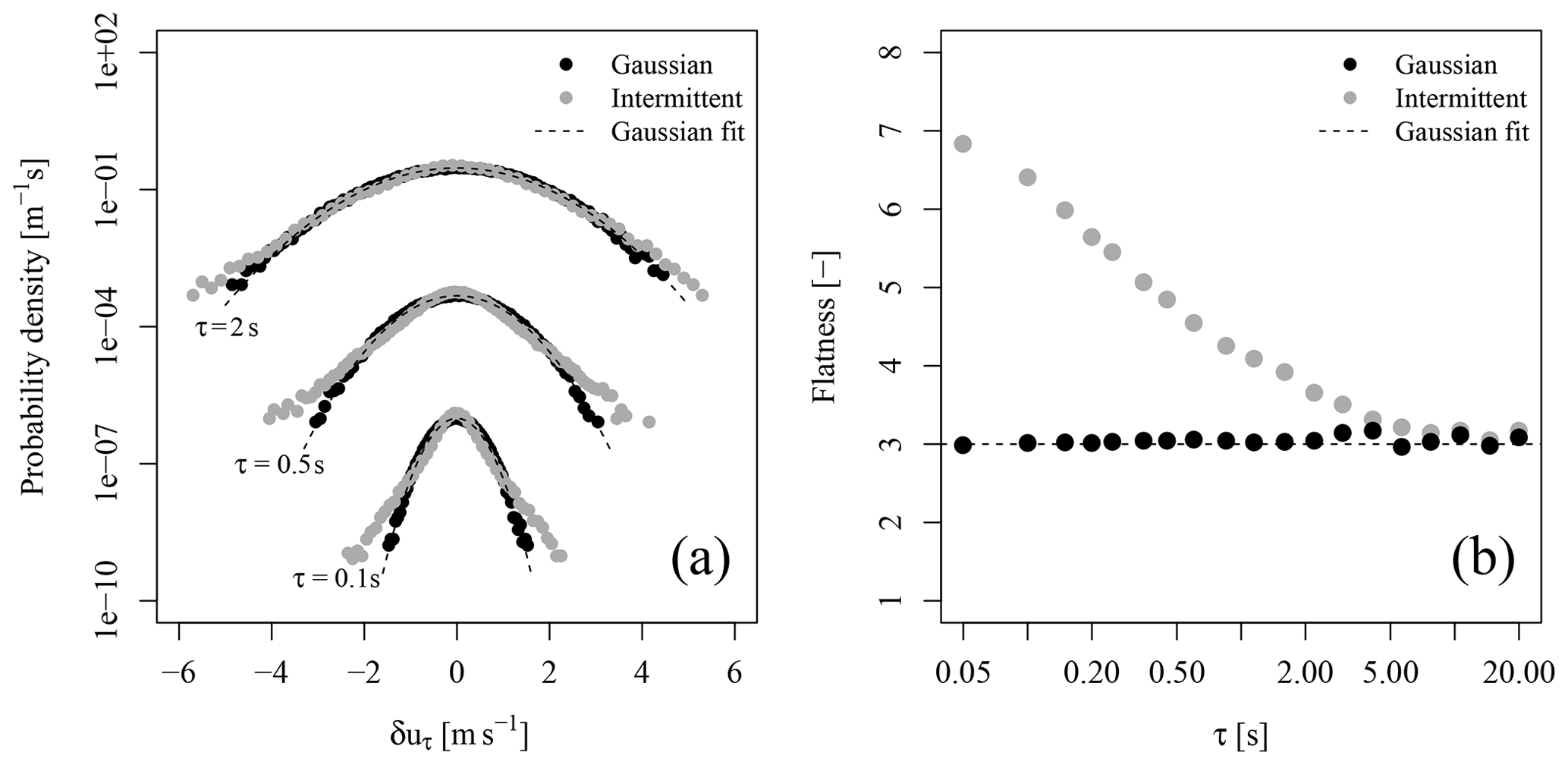
Figure 5Comparison of the two-point statistics for the Gaussian and intermittent fields. (a) Histograms of velocity increment time series for τ=0.1, 0.5, 2 s, shifted vertically for better representation. (b) Flatness of increment PDFs in the range 0.05 s 15 s.
Up until now, no differences between both types of wind fields were evident. This changes when the PDFs of 2P statistics are considered: the non-Gaussianity of the 2P statistics is displayed in Fig. 5. Figure 5a shows the histograms of wind velocity increments δuτ for τ={0.05, 0.1, 2}. A deviation from an ideal Gaussian process is evident for the intermittent data set. The deviation is dependent on the time lag τ between the two points considered. In order to describe the scale dependency and the deviation from an ideal Gaussian PDF, Fig. 5b represents the fourth moment (alias flatness or kurtosis) of increment PDFs in dependence of τ. As can be seen, the increment statistics of the intermittent data sets deviate from a Gaussian process in the range τ<10 s.
The fourth moment of the 2P statistics is the lowest-order statistic in which differences between the two types of fields are evident.
2.1.3 Spatial dynamics
The statistical features presented in the previous section could be achieved for isolated velocity time series u(t) but not for time series in a spatially correlated fields. In order to assemble velocity fields u(y, z, t), simplified spatial correlations are considered.
Firstly, we generate a field in which in all grid points are prescribed the same time series. This case is referred to as the spatially fully correlated case. Secondly, a grid is filled with different, uncorrelated time series, which are independent from another, referred to as the spatially delta-correlated case.
These are strongly idealized scenarios. Commonly, a spectrum of structure sizes is expected for realistic wind fields. For reference, integral length scales on the order of several hundred metres (Träumner et al., 2015) have been reported. We therefore argue that a realistic wind field at times may approach one or the other of these extreme scenarios and most of the time will feature moderate correlations, which are bounded by the two extremes. In order to provide wind fields in between both of these extreme scenarios, a subdivided 3×3 grid is considered. In the resulting nine subregions, we prescribe fully correlated fields. These three cases are illustrated in Fig. 6.
The resulting correlations and coherence must be understood as a simplification of atmospheric turbulence, as it features a varying range of temporal and spatial scales. Since only regularized structures of one size are featured in the field, only the corresponding scales are contained in the fields. Implementing a more realistic coherence model into the CTRW model is very challenging: coherence is typically incorporated by combining spectral properties of different grid points. However, these spectral properties correspond to the second moment of velocity increments via the Wiener–Khinchin theorem. Therefore, it is not possible or highly difficult to conserve all of the targeted properties of our wind time series when trying to implement coherence in the spirit of the Veers method (Veers, 1988). We believe this will have an impact on our results, mainly in a quantitative way: coherence typically introduces the spatial variation in the wind field, which leads to the so-called “eddy slicing” by the rotor, which in return is a driver for fatigue loads. This effect is not fully captured in our approach, wherefore the resulting load dynamics will feature less contributions for eddy slicing. However, we do not see the qualitative nature of our findings to be affected by these simplifications.

Figure 6Exemplary visualization of the flow field excerpts for a mean velocity in the main flow direction of u=12.5 m s−1: (a) Gaussian type, fully correlated in space; (b) Gaussian type, 3×3 subdivision in space; (c) Gaussian type, delta correlated in space.
2.2 Wind turbine model
The wind fields generated in this study were applied in simulations of a common pitch-regulated wind turbine. As a test wind turbine, the well-documented National Renewable Energy Laboratory (NREL) 5 MW reference wind turbine, with a rated wind speed of 11.4 m s−1, was selected (Jonkman et al., 2009). Aero-servo-elastic simulations were carried out using FAST (Jonkman and Buhl, 2005; Jonkman and Jonkman, 2016) (v8.15), including its BEM code AeroDyn15 (v15.02) (Jonkman et al., 2016). Active pitch and variable speed control, as well as common add-ons to the pure BEM model for, e.g. tip losses or the tower effect are taken into consideration by application of typical correction models.
BEM theory is based on stationary airfoil data and further on an equilibrium wake (Schepers, 2012). Dynamic airfoil behaviour is modelled with a Beddoes and Leishman type of dynamic stall model with minor code-specific modifications (Leishman and Beddoes, 1989; Jonkman et al., 2016). Generally, it is an open question how well load dynamics resulting from turbulent inflow are captured by a BEM method. However, Madsen et al. (2018) recently presented evidence that BEM codes are capturing general trends well.
2.3 Load analysis
The resulting wind fields are analysed with respect to the load response of a wind turbine model. The so-obtained load time series can be analysed in manifold ways. In this work, we focus on fatigue loads, as these are dependent on the entirety of the wind and load statistics. A specific methodology is proposed by certification guidelines, such as International Electrotechnical Commission (2005) for this kind of load analysis. Following International Electrotechnical Commission (2005), a RFC procedure (Matsuishi and Endo, 1968) is conducted. In doing so, a load history is simplified into a sequence of local load maxima. Subsequently, so-called load ranges ri are calculated from this sequence. Load ranges are essentially load increments similar to Eq. (1) but calculated exclusively between local load extrema. The resulting load ranges ri are utilized to calculate an EFL:
where ri is the ith load range and T represents the number of seconds covered by the load history. Due to the selection of T, this specific load is referred to as the 1 Hz EFL. Further, m is the SN-slope coefficient (in this study, mTow=4 for the tower, mDrvTr=8 for drive train components and mBld=12 for the blades). Intuitively, the EFL can be understood as the peak-to-peak amplitude of a hypothetical load cycle with the period of 1 s, which leads to the same damage accumulation as the input load history over the time T.
Note that, in practice, the EFL is calculated over a wide range of wind speeds. The wind-specific fatigue loads are subsequently combined with a wind probability distribution and integrated up, so that finally one value for the entire lifetime is obtained. In this work, we focus on the loading at specific wind speeds in order to identify potential trends.
Due to the limited scope of this paper, not all turbine components and load sensors can be discussed here. We focus mainly on load sensors that are expected to be responsive to wind dynamics and not dominated by other effects, such as gravitational forces. The two sensors presented here exemplarily are the rotor thrust and the tower-base-bending moment fore–aft (TBMFA).
This section is organized as follows: firstly, the fully correlated wind field case is discussed. Subsequently, this result is compared against the results from the delta-correlated case, and the intermediate 3×3 case is discussed at last. Finally, 2P load statistics for all cases are compared to underline the impact of the spatial dynamics and the coherence of the wind field.
3.1 Results for fully correlated fields
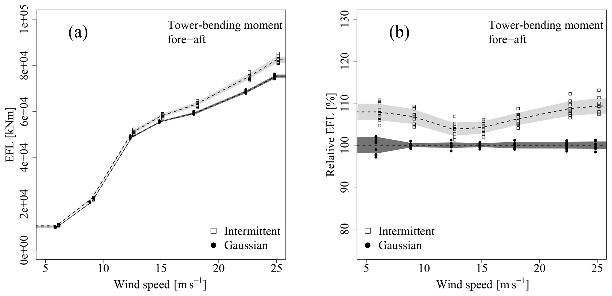
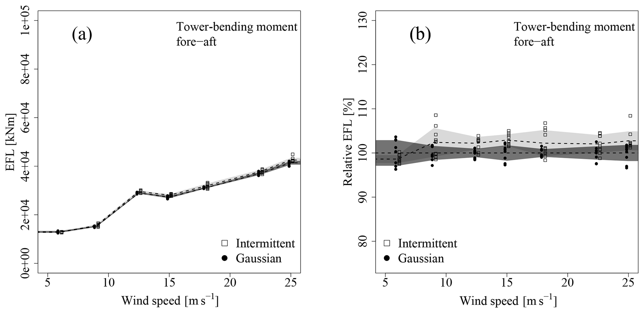
Figures 7 and 8 show the comparison of EFLs obtained for the Gaussian and intermittent fields for the fully correlated case in absolute and relative values for the rotor thrust and TBMFA. Differences between intermittent and Gaussian types for both sensors are evident in the case of fully correlated fields at all wind speeds. As a rough overall trend, the intermittent cases seem to yield a 5 % to 10 % increase in fatigue loads, which can be relevant in a design or certification process. Due to the isolation of intermittency discussed in Sect. 2.1.2, this difference can directly be associated with the intermittent statistics.
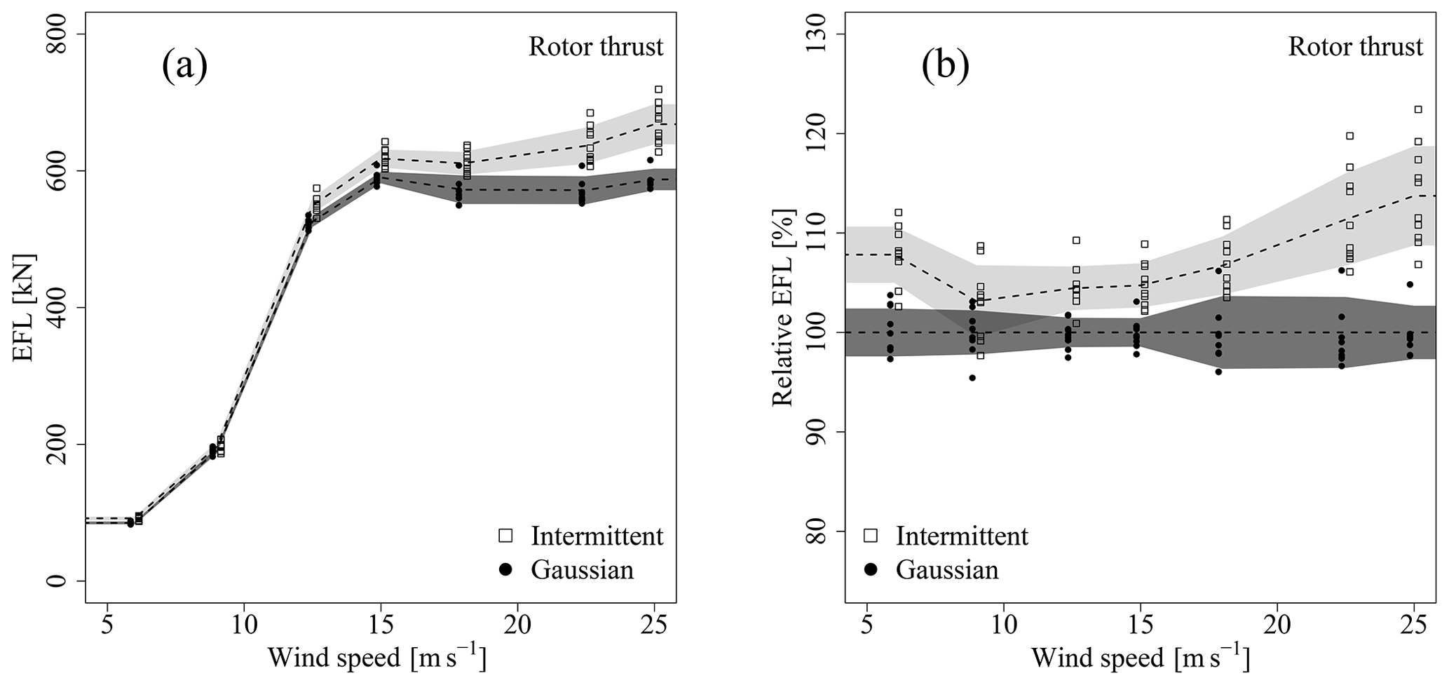
Figure 7EFL (see Eq. 4) for the rotor thrust for all realizations and all wind speeds for the fully correlated case. The data points were shifted horizontally for a better distinction between intermittent and Gaussian data. The dashed lines represent averages; the shaded area covers ± 1 standard deviation around the average. (a) Standard representation. (b) Data are normalized with the average of the Gaussian result (Gaussian averages correspond to 100 %).
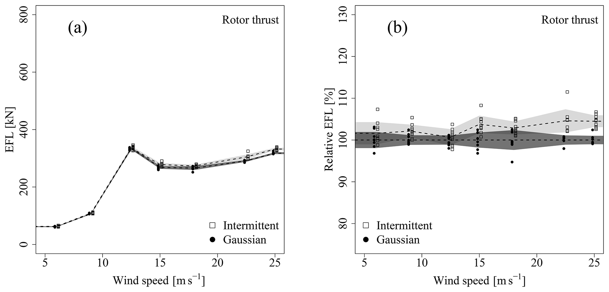
3.2 Results for delta-correlated fields
Next, the delta-correlated wind fields are considered. Figures 9 and 10 show the comparison for the delta-correlated case for the rotor thrust and TBMFA. It is evident that there is no significant difference between the Gaussian and intermittent wind fields. Physically, this behaviour can be explained, as the blades are excited by a multitude of uncorrelated processes over the course of a rotor revolution. The dynamics of rotational sampling of the spatial variations outweigh the effect of the temporal statistics.
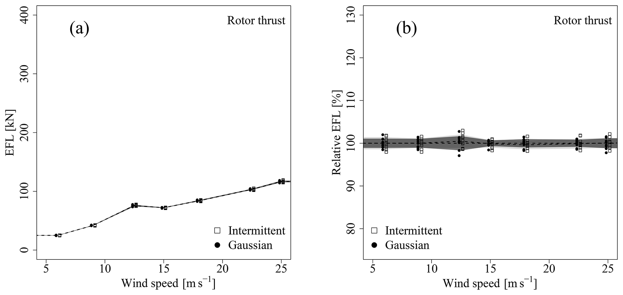
Figure 9EFL for the rotor thrust for the delta-correlated case. The figure is analogous to Fig. 7.
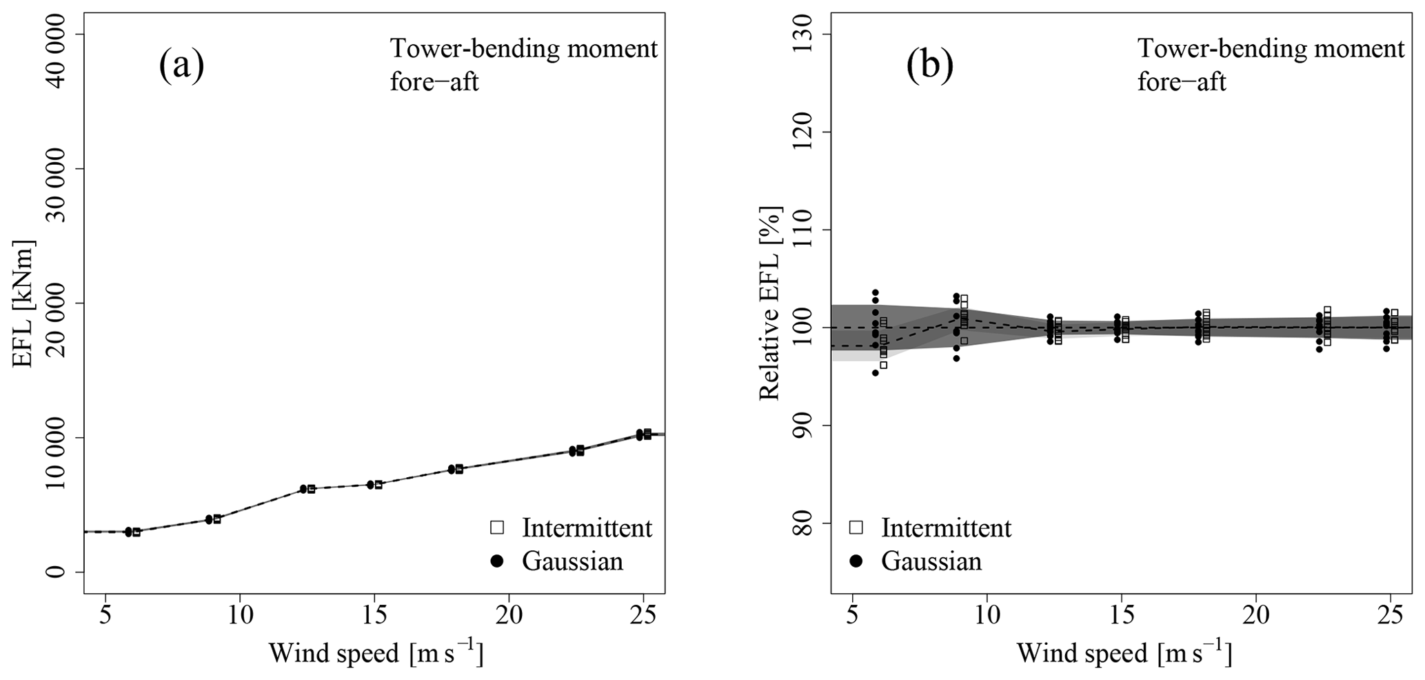
Figure 10EFL for the TBMFA for the delta-correlated case. The figure is analogous to Fig. 7.
3.3 Results for subdivided 3×3 field
Finally, an intermediate case between the fully and delta-correlated wind fields is presented. Results are shown in Figs. 11 and 12. For both sensors, differences between the Gaussian and intermittent cases are still evident. However, these are much less pronounced than for the fully correlated case. In contrast to the delta-correlated case, however, differences can be identified.
3.4 Load increment statistics
In order to show to which degree the intermittent wind dynamics affect the load dynamics in each of the three types of wind fields, the statistics of the load increments xτ (see Eq. 1) are discussed. In this context, x denotes any load sensor. Figure 13 shows the flatness of the resulting rotor thrust and TBMFA increments at 12.5 m s−1.
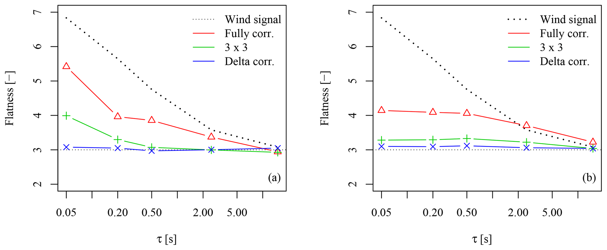
Figure 13Flatness of load increment PDFs for intermittent fields with different spatial dynamics: (a) for the rotor thrust; (b) for the TBMFA.
It is evident that for the fully correlated case, the non-Gaussianity of the wind signal is induced into the rotor thrust. Deviations from the wind statistics of uτ can be explained by the complex and non-linear aero-servo-elastic response of the rotor thrust signal to the incoming wind dynamics. These are individual for each load sensor, as can be seen when comparing the thrust signal with the TBMFA signal in Fig. 13a and b, respectively.
In the delta-correlated case, the load signal becomes almost perfectly Gaussian (flatness of 3). The Gaussianity of these load dynamics can be explained with the central limit theorem: the rotor is excited by uncorrelated random variables over the course of one revolution. The superposition of all of these processes yields a regular and steady Gaussian dynamic.
Lastly, the 3×3 subdivision is considered. Comparable to the EFL results, the load increments for this field type feature some remaining non-Gaussianity; however, it is much lower compared to the fully correlated case.
At this point, we need to recall that all three spatial compositions are idealizations. A real wind field features structures up to length scales of several hundred metres (Träumner et al., 2015), as the fully correlated case. However, it also features structures of small size as in the delta-correlated case. However, it will contain more than one structure size. It thus remains an open question of which cases represents real wind fields most adequately.
This work adds to the discussion of intermittency in the context of wind turbine dynamics as follows:
-
In order to evaluate the impact of higher-order statistics or intermittency in wind dynamics, they need to be isolated properly. An example of such an isolation has been given in this work.
-
Intermittent wind dynamics and advanced wind statistics can be relevant to the fatigue loads of wind turbines. This holds true for an aero-servo-elastic wind turbine response including pitch control and variable rotor speeds. An effect on the purely aerodynamic response has been reported in Schwarz et al. (2018).
-
The quantitative values presented in this work have to be treated with caution due to the simplified spatial correlations in the wind fields. Still, to provide a quantitative estimate, the lifetime fatigue has been calculated based on a wind class III Weibull distribution (shape is 2; scale is 8.46). The relative increase in fatigue due to intermittency for the rotor thrust equates to 105.7 % (fully correlated), 102.3 % (3×3 case) and 100.2 % (delta correlated).
-
The intermittency effect depends on the size and number of wind structures, also referred to as the coherence of the field. Highly coherent fields show an intermittency effect, incoherent fields do not. The dependence on spatial variation needs to be investigated further.
The generated wind fields, time series, as well as the necessary processing scripts and wind turbine model may be obtained by contacting the corresponding author.
For details and other deployments of this model, the reader may refer to Kleinhans et al. (2008); Kleinhans (2008), Mücke et al. (2011) and Gontier et al. (2007). Time series generation in the CTRW model is based on two coupled Ornstein–Uhlenbeck (OU) processes and stochastic mapping.
The OU processes are
and
In the previous equations,
Γ represents white noise.
The stochastic mapping process s→t is realized as
where τα,C is a bounded stochastic process yielding Lévy distributed random numbers in the range . Note , so that s=t and ui(s)=ui(t). An implementation of such a process can be achieved as
with V being a uniformly distributed random variable in the range [, ] and W an exponential distribution with unit mean.
Constants are
CMS generated the wind fields, conducted the simulations and the load analysis and wrote the manuscript. SE refined the wind model and was equally involved with the generation of the wind fields and interpretation of the results. JP had the initial idea, supervised the work and helped in preparing the manuscript.
The authors declare that they have no conflict of interest.
The authors would like to thank the editor and referees for their helpful comments and remarks.
This research has been supported by the European Union's Seventh Framework Programme (grant nos. FP7-ENERGY-2013-1 and 608396).
This paper was edited by Jakob Mann and reviewed by Jacob Berg and Vasilis A. Riziotis.
Berg, J., Natarajan, A., Mann, J., and Patton, G.: Gaussian vs non-Gaussian turbulence: impact on wind turbine loads, Wind Energy, 19, 1975–1989, https://doi.org/10.1002/we.1963, 2016. a, b, c, d
Böttcher, F., Renner, C., Waldl, H., and Peinke, J.: Problematik der Windböen, DEWI Magazin, 19, 58–62, 2001. a
Böttcher, F., Renner, C., Waldl, H., and Peinke, J.: On the statistics of wind gusts, Bound.-Lay. Metereol., 108, 163–173, 2003. a, b, c, d
Gontier, H., Schaffarczyk, A. P., Kleinhans, D., and Friedrich, R.: A comparison of fatigue loads of wind turbine resulting from a non-Gaussian turbulence model vs. standard ones, J. Phys.: Conf. Ser., 75, 012070, https://doi.org/10.1088/1742-6596/75/1/012070, 2007. a, b, c
Hähne, H., Schottler, J., Waechter, M., Peinke, J., and Kamps, O.: The footprint of atmospheric turbulence in power grid frequency measurements, Europhys. Lett., 121, 30001, https://doi.org/10.1209/0295-5075/121/30001, 2018. a, b
International Electrotechnical Commission: IEC 61400, 2005. a, b, c, d, e
Jonkman, B. and Jonkman, J.: FAST v8.16.00a-bjj, Tech. rep., NREL, available at: https://wind.nrel.gov/nwtc/docs/README_FAST8.pdf (last access: 1 November 2019), 2016. a
Jonkman, J. M. and Buhl, M. L.: FAST User's Guide, Tech. Rep. EL-500-38230, National Renewable Energy Laboratory, Colorado, 2005. a
Jonkman, J. M., Butterfield, S., Musial, W., and Scott, G.: Definition of a 5-MW Reference Wind Turbine for Offshore System Development, Tech. Rep. TP-500-38060, National Renewable Energy Laboratory, Golden, CO, USA, 2009. a
Jonkman, J. M., Hayman, G., Jonkman, B., and Damian, R.: AeroDyn v15 User's Guide and Theory Manual (draft version), Tech. rep., NREL, available at: https://wind.nrel.gov/nwtc/docs/AeroDyn_Manual.pdf (last access: 1 November 2019), 2016. a, b
Kaimal, J. C., Wyngaard, J. C., Izumi, Y., and Cote, O. R.: Spectral characteristics of surface-layer turbulence, Q. J. Roy. Meteorol. Soc., 98, 563–598, 1972. a, b, c, d
Kleinhans, D.: Stochastische Modellierung komplexer Systeme, PhD thesis, Westfälische Wilhelms-Universität Münster, Münster, 2008. a, b, c, d, e, f, g, h
Kleinhans, D., Friedrich, R., Gontier, H., and Schaffarczyk, A.: Simulation of intermittent wind fields: A new approach, in: The 8th International Technical Wind Energy Conference, DEWEK 2006, 22–23 November 2006, Bremen, Germany, 2008. a, b, c
Kolmogorov, A.: Dissipation of energy in the locally isotropic turbulence, Dokl. Akad. Nauk SSSR, 434, https://doi.org/10.1098/rspa.1991.0076, 1941. a, b
Körber, F., Besel, G., and Reinhold, H.: Meßprogramm an der 3 MW-Windkraftanlage GROWIAN: Schlußbericht, Abschlußdatum: 31.12.1987, Contract 03-E-4512-Awindb, Tech. rep., Bundesministerium für Forschung und Technologie, Statusreport Windenergie, Veranstaltung der Projektleitung Biologie, Oekologie und Energie der KFA Juelich im Auftrage des BMFT, Luebeck, 1–2 March 1988 and can now be accessed through the Technische Informationsbibliothek (TIB), Hannover, 1988. a
Kutner, R. and Jaume, M.: The continuous time random walk, still trendy: fifty-year history, state of art and outlook, Eur. Phys. J. B, 90, 50–63, https://doi.org/10.1140/epjb/e2016-70578-3, 2017. a
Leishman, J. G. and Beddoes, T. S.: A Semi-Empirical Model for Dynamic Stall, J. Am. Helicopt. Soc., 34, 3–17, 1989. a
Madsen, H. A., Sørensen, N. N., Bak, C., Troldborg, N., and Pirrung, G.: Measured aerodynamic forces on a full scale 2 MW turbine in comparison with EllipSys3D and HAWC2 simulations, J. Phys.: Conf. Ser., 1037, 022011, https://doi.org/10.1088/1742-6596/1037/2/022011, 2018. a
Mann, J.: The spatial structure of neutral atmospheric surface-layer turbulence, J. Fluid Mech., 273, 141–168, 1994. a, b, c
Matsuishi, M. and Endo, T.: Fatigue of Metals Subjected to Varying Stress, Paper presented to Japan Society of Mechanical Engineers, Fukuoka, Japan, March 1968. See also: Endo, T., et. al., “Damage Evaluation of Metals for Random or Varying Loading”, in: Proceedings of the 1974 Symposium on Mechanical Behavior of Materials, Vol. 1, Society of Materials Science, Kyoto, Japan, 371–380, 1968. a, b
Milan, P., Wäechter, M., and Peinke, J.: Turbulent Character of Wind Energy, Phys. Rev. Lett., 110, 138701, https://doi.org/10.1103/PhysRevLett.110.138701, 2013. a, b
Montroll, E. W. and Weiss, G. H.: Random Walks on Lattices. II, J. Math. Phys., 6, 167–181, https://doi.org/10.1063/1.1704269, 1965. a
Morales, A., Wächter, M., and Peinke, J.: Characterization of wind turbulence by higher-order statistics, Wind Energy, 15, 391–406, https://doi.org/10.1002/we.478, 2012. a, b, c
Mücke, T., Kleinhans, D., and Peinke, J.: Atmospheric turbulence and its influence on the alternating loads on wind turbines, Wind Energy, 14, 301–316, 2011. a, b, c, d, e, f, g
Powell, D. C. and Connell, J. R.: Review of Wind Simulation Methods For Horizontal-Axis Wind Turbine Analysis, Tech. Rep. PNL-5903, Battelle Pacific Northwest Laboratory, Richland, Washington, USA, 1986. a
Schepers, J. G.: Engineering models in wind energy aerodynamics, PhD thesis, Technische Universiteit Delft, Delft, 2012. a
Schottler, J., Reinke, N., Hölling, A., Whale, J., Peinke, J., and Hölling, M.: On the impact of non-Gaussian wind statistics on wind turbines – an experimental approach, Wind Energy Sci., 2, 1–13, https://doi.org/10.5194/wes-2-1-2017, 2017. a, b
Schwarz, C. M., Ehrich, S., Martín, R., and Peinke, J.: Fatigue load estimations of intermittent wind dynamics based on a Blade Element Momentum method, J. Phys.: Conf. Ser., 1037, 07204, https://doi.org/10.1088/1742-6596/1037/7/072040, 2018. a, b, c
Thomas, P., Wächter, M., Alexandros, A., and Jersch, T.: InterWiLa Schlussbericht: Berechnung und Validierung von Lasten an Windenergieanlagen aufgrund intermittenter Windfelder, Tech. Rep. 0325798A, 0325798B, 01158023, Fraunhofer-Institut für Windenergie und Energiesystemtechnik (IWES), Bremerhaven, 2017. a
Träumner, K., Damian, T., Stawiarski, C., and Wieser, A.: Turbulent Structures and Coherence in the Atmospheric Surface Layer, Bound.-Lay. Meteorol., 154, 1–25, https://doi.org/10.1007/s10546-014-9967-6, 2015. a, b
Veers, P.: Three-Dimensional Wind Simulation, Tech. Rep. SAND88-0152 UC-261, United States Department of Energy, Sandia National Laboratories Albuquerque, New Mexico and Livermore, California, 1988. a, b
Vindel, J. M., Yagüe, C., and Redondo, J. M.: Structure function analysis and intermittency in the atmospheric boundary layer, Nonlin. Processes Geophys., 15, 915–929, https://doi.org/10.5194/npg-15-915-2008, 2008. a, b
Wächter, M., Heißelmann, H., Hölling, M., Morales, M., Milan, P., Mücke, T., Peinke, J., Reinke, N., and Rinn, P.: Wind Energy and the Turbulent Nature of the Atmospheric Boundary Layer, J. Turbul., 13, 1–21, https://doi.org/10.1080/14685248.2012.696118, 2012. a