On the self-similarity of wind turbine wakes in a complex terrain using large eddy simulation

We perform large eddy simulation of flow in a complex terrain under neutral atmospheric stratification. We study the self-similar behavior of a turbine wake as a function of varying terrain complexity and perform comparisons with a flat terrain. By plotting normalized velocity deficit profiles in different complex terrain cases, we verify that self-similarity is preserved as we move downstream from the turbine. We find that this preservation is valid for a shorter distance downstream compared to what is observed in a flat terrain. A larger spread of the profiles toward the tails due to varying levels of shear is also observed.

1 Introduction

Rotor wakes have a consequential impact on the efficiency of a wind farm, as the turbines standing in wake generally face lower wind speeds along with enhanced turbulence levels (Barthelmie et al., 2007). The particular dynamics of wakes are strongly influenced by the terrain characteristics, such as surface vegetation and sloping terrain. Although a lot of emphasis has been on understanding wakes in flat terrain over the past decade (Medici and Alfredsson, 2006; Jimenez et al., 2007; Chamorro and Porté-Agel, 2009; Iungo et al., 2013; Calaf et al., 2010; Porté-Agel et al., 2011; Abkar et al., 2016; Allaerts and Meyers, 2015; Iungo, 2016), complex terrains now finally get the attention they deserve. This is partly due to a prospective shift in development of wind farms from flat to complex terrains caused by saturation of ideal flat terrains and increasing development of wind energy over the past 2 decades (Alfredsson and Segalini, 2017; Feng et al., 2017); it is also partly due to the recent observational and numerical developments. Understanding wakes from turbines in complex terrains, therefore, becomes important for understanding the interaction between terrain and wakes, as well as for better resource assessment and wind farm siting. The change in topography gives rise to flow phenomenon such as speed-up across the hills, flow separation behind hills with high slopes and generation of localized turbulent structures. This makes flow prediction in complex terrains challenging and turbine behavior in such locations is far from understood.

Recent works on wake interaction in complex terrains either deal with the topic in ideal complex terrains such as Gaussian or sinusoidal hills or present site-specific studies. Tian et al. (2013) performed an experimental study of five turbines located on a Gaussian two-dimensional hill to understand the interaction of wind farm with the terrain. Their experimental setup was numerically regenerated in a large eddy simulation (LES) domain by Shamsoddin and Porté-Agel (2017) in an attempt to validate their LES model. Hyvarinen and Segalini (2017) also studied wakes over periodic sinusoidal hills. Using experimental and numerical tools, they achieved good agreement between the two; however, implementing the Jensen wake model (Katic et al., 1986) did not yield good results.

Coming to the site-specific studies, Castellani et al. (2017) studied the impact of wakes and terrain on the performance of a wind farm located in southern Italy. Lutz et al. (2017) used detached eddy simulation to study the wake from a single turbine in a complex site in Germany. The impact of topography on wake development was highlighted by comparison with a flat terrain case. Recently, Berg and coworkers performed a large eddy simulation study of wake from a wind turbine located at the site of Perdigão, Portugal (Berg et al., 2017), and highlighted some differences in wake orientation from Shamsoddin and Porté-Agel's work (Shamsoddin and Porté-Agel, 2017). From analyzing wind scanner data from Perdigão, Menke et al. (2018) show a strong influence of atmospheric stability on wake propagation and orientation. This further supports the hypothesis that it is difficult to generalize wind turbine wake results for complex sites.

The velocity deficit profiles as a function of downstream distance in the wake collapse on a single profile when scaled with the maximum deficit and characteristic wake-width; this property is known as self-similarity. Wakes behind turbines are known to show self-similar behavior in a flat terrain under different atmospheric conditions. Xie and Archer (2014) showed mean velocity deficit behind turbines to be self-similar in neutral conditions. Abkar and Porté-Agel (2015) found self-similarity under various stability classes. This was further explored by Xie and Archer (2017), who then checked for self-similarity under different stability conditions in the presence of the Coriolis force. This self-similar behavior of mean velocity deficit in the far wake has been a fundamental assumption for many analytical wake models (Katic et al., 1986; Xie and Archer, 2014; Abkar and Porté-Agel, 2015; Bastankhah and Porté-Agel, 2014).

In the current work, we look for self-similarity of wind turbine wakes in a complex terrain under neutral atmospheric conditions and without the effect of the Coriolis force. For this purpose, we extend the work by Berg et al. (2017) and verify self-similarity of wakes under different terrain characteristics and turbine locations. If successful, this can potentially provide a basis for the development of analytical models for wakes in complex terrains (Luzzatto-Fegiz, 2018). This self-similarity of rotor wakes in complex terrains has not yet been verified in the existing literature to the best of the authors' knowledge.

The rest of the paper is structured as follows: Sect. 2 details the LES code used for the study; terrain characteristics along with case configuration and data descriptions are provided in Sect. 3. A nomenclature for wake statistics necessary for the self-similarity check is presented in Sect. 4, and results from the study are shown in Sect. 5. The paper is finally concluded in Sect. 6.

2 LES framework

The large eddy simulation code used in the current study is formerly formulated in Sullivan et al. (2014) with examples of usage in complex terrains in Sullivan et al. (2010). The governing equations are the spatially filtered incompressible Navier–Stokes and continuity equations, which for a neutrally stratified atmospheric flow read as

$$\begin{array}{}\text{(1)}& {\displaystyle }& {\displaystyle \frac{\partial \stackrel{\mathrm{̃}}{u_i}}{\partial x_i}}=\mathrm{0},\text{(2)}& {\displaystyle }& {\displaystyle \frac{\partial \stackrel{\mathrm{̃}}{u_i}}{\partial t}}+{\displaystyle \frac{\partial \stackrel{\mathrm{̃}}{u_i}\stackrel{\mathrm{̃}}{u_j}}{\partial x_j}}=-\left[{\displaystyle \frac{\partial {\stackrel{\mathrm{̃}}{p}}^{*}}{\partial x_i}}+{\displaystyle \frac{f_i}{\mathit{\rho }}}+{\displaystyle \frac{\partial {\mathit{\tau }}_{ij}}{\partial x_j}}\right]+F_{\mathrm{p}}{\mathit{\delta }}_{i\mathrm{1}},\end{array}$$

where $\stackrel{\mathrm{̃}}{u_i}$ is the resolved velocity in x, y and z directions corresponding to i={1, 2, 3}, respectively. The pressure variable ${\stackrel{\mathrm{̃}}{p}}^{*}$ is solved using the elliptic Poisson equation in an iterative manner. f_i is the body force which models the interaction of the turbine with the flow and ρ is the fluid density, which is kept constant throughout the study. The kinematic subgrid scale stresses are represented by ${\mathit{\tau }}_{ij}=\stackrel{\mathrm{̃}}{u_i{u}_j}-\stackrel{\mathrm{̃}}{u_i}\stackrel{\mathrm{̃}}{u_j}$. The external forcing driving the flow is represented by F_p, which in the current case is the constant pressure gradient in the streamwise direction (see later text). An important thing to note is that the Coriolis and buoyancy forces are neglected in the current study.

A terrain-following coordinate transformation is used to represent the complex geometry. The transformation that maps physical coordinates, x_i=(x, y, z), onto computational coordinates, ξ_i=(ξ, η, ζ), x_i⇒ξ_i, is given by the following rules:

$$\begin{array}{}\text{(3)}& {\displaystyle }& {\displaystyle }\mathit{\xi }=\mathit{\xi }\left(x\right)=x,\text{(4)}& {\displaystyle }& {\displaystyle }\mathit{\eta }=\mathit{\eta }\left(y\right)=y,\text{(5)}& {\displaystyle }& {\displaystyle }\mathit{\zeta }=\mathit{\zeta }(x,y,z),\end{array}$$

with the corresponding Jacobian given by

$$\begin{array}{}\text{(6)}& \mathbf{J}=\det \left[\begin{array}{ccc}{\mathit{\xi }}_x& \mathrm{0}& \mathrm{0}\\ \mathrm{0}& {\mathit{\eta }}_y& \mathrm{0}\\ {\mathit{\zeta }}_x& {\mathit{\zeta }}_y& {\mathit{\zeta }}_z\end{array}\right]={\mathit{\xi }}_x{\mathit{\eta }}_y{\mathit{\zeta }}_z={\mathit{\zeta }}_z,\end{array}$$

where the subscript denotes partial derivative. The governing equations, Eqs. (1) and (2), can now be transformed using the chain rule and the identity (consult Sullivan et al., 2014, for details),

$$\begin{array}{}\text{(7)}& {\displaystyle \frac{\partial }{\partial {\mathit{\xi }}_j}}\left({\displaystyle \frac{\mathrm{1}}{J}}{\displaystyle \frac{\partial {\mathit{\xi }}_j}{\partial x_i}}\right)=\mathrm{0},\end{array}$$

in order to write a set of equations in a strong flux-conservation form using the volume flux variables,

$$\begin{array}{}\text{(8)}& U_i={\displaystyle \frac{\stackrel{\mathrm{̃}}{u_j}}{J}}{\displaystyle \frac{\partial {\mathit{\xi }}_i}{\partial x_j}},\end{array}$$

so that U_i=(U, V, W) is normal to surfaces of constant ξ_i. In the numerical mesh, W is located on cell faces, while U and V are located in cell centers. This ensures a tight coupling to pressure defined at the cell centers. Solving the Poisson equation involves an iteration procedure which incurs additional expense compared to conventional computations in flat terrain (again we recommend the reader to consult Sullivan et al., 2014, for details).

The code is pseudo-spectral code, with wave number representation in the horizontal directions (ξ, η), and 2nd-order finite difference in the vertical direction, ζ.

The physical (z) and computational (ζ) vertical coordinates are related to each other using a simple transformation rule, with z exponentially stretched from the surface:

$$\begin{array}{}\text{(9)}& \mathit{\zeta }=H{\displaystyle \frac{z-h}{H-h}},\end{array}$$

where h=h(x, y) is the local terrain height and H is the domain height.

The Deardorff SGS (subgrid scale) model as adopted in Moeng (1984); Sullivan et al. (1994) is implemented to parameterize the subgrid scale stresses.

Turbine parameterization

An actuator disk model without any rotational effects is implemented to represent the turbines. The unavailability of a well defined free stream velocity, U_∞, in complex terrain is compensated by employing the classical expression given by Hansen (2015) and introduced into actuator disk representation in LES by Calaf et al. (2010):

$$\begin{array}{}\text{(10)}& U_{\mathrm{\infty }}={\displaystyle \frac{{\stackrel{\mathrm{‾}}{u}}_{\mathrm{d}}}{\mathrm{1}-a}},\end{array}$$

where ${\stackrel{\mathrm{‾}}{u}}_{\mathrm{d}}$ is the velocity averaged over the rotor disk and a is the axial induction factor. The model simulates turbines using disks with a thrust force given by

$$\begin{array}{}\text{(11)}& F_{\mathrm{T}}=-{\displaystyle \frac{\mathrm{1}}{\mathrm{2}}}\mathit{\rho }{C}_{\mathrm{T}}^{\prime }{\stackrel{\mathrm{‾}}{u}}_{\mathrm{d}}^{\mathrm{2}}{\displaystyle \frac{\mathit{\pi }}{\mathrm{4}}}{D}^{\mathrm{2}},\end{array}$$

where D is the rotor diameter and $C_{\mathrm{T}}^{\prime }$ is related to the thrust coefficient C_T using one-dimensional momentum theory:

$$\begin{array}{}\text{(12)}& C_{\mathrm{T}}^{\prime }={\displaystyle \frac{C_{\mathrm{T}}}{(\mathrm{1}-a{)}^{\mathrm{2}}}}={\displaystyle \frac{\mathrm{4}a}{(\mathrm{1}-a)}}.\end{array}$$

For the current work, we choose an induction, $a=\mathrm{1}/\mathrm{4}$, which corresponds to $C_{\mathrm{T}}^{\prime }=\mathrm{4}/\mathrm{3}$. In the numerical code, the thrust force is then distributed proportionally to the fractional area of each cell covered by the rotor. The force per unit volume in the longitudinal direction is then given by

$$\begin{array}{}\text{(13)}& f_x(i,j,k,t)=-{\displaystyle \frac{\mathrm{1}}{\mathrm{2}}}\mathit{\rho }{C}_{\mathrm{T}}^{\prime }{\stackrel{\mathrm{‾}}{u}}_{\mathrm{d}}(t{)}^{\mathrm{2}}{\displaystyle \frac{\mathrm{\Lambda }(j,k)}{\mathrm{\Delta }x}},\end{array}$$

where Λ is the fractional area and Δx is length of a given cell. In the implementation, we have added a 10 min exponential time filter to ${\stackrel{\mathrm{‾}}{u}}_{\mathrm{d}}$.

3 Case configurations

Simulations are performed on a domain spanning over $\mathrm{5120}\mathrm{m}\times \mathrm{2560}\mathrm{m}\times \mathrm{3000}$ m, which represents a double-ridge-configured site named Perdigão in Portugal (Vasiljević et al., 2017). The site has been the focus of an intensive field measurement campaign under the Perdigão experiment 2017 (Wildmann et al., 2018; Menke et al., 2018) and the New European Wind Atlas (NEWA) project (Mann et al., 2017). Fig. 1a shows the overview of the site, where the wind direction is along the main transect (235^∘ relative to north). With its double ridge configuration and challenging slopes, the terrain is ideal for a comprehensive study of interaction between wind turbine wake and topography. In Fig. 1b we show the numerical terrain. In order to make the terrain periodic to comply with the pseudo-spectral LES model, a little smoothing had to be performed. The atmosphere is assumed to be neutrally stratified and boundary conditions used are described below. A roughness length of z₀=0.5 m is chosen, keeping the rugged, forested terrain in mind, giving $z_{\mathrm{0}}/H=\mathrm{1.67}\times {\mathrm{10}}^{-\mathrm{4}}$. The simulations are initiated from a random incompressible velocity field and run for a time of T_S=100T_E until stationarity was achieved. Here, $T_{\mathrm{E}}=H/u_{*}$ (u_* is defined as friction velocity) is the timescale corresponding to the size of the largest eddy that can possibly fit in the domain and is based on a simple momentum transfer argument borrowed from the flat terrain. Figure 2 shows an instantaneous snapshot of streamwise velocity along the main transect passing through the turbine located on top of the first ridge with respect to flow direction. The turbine is assumed to have a rotor diameter and hub height of 80 m each. This is done to somewhat match the dimensions of an ENERCON 2 MW turbine actually deployed at the upwind ridge at Perdigão.

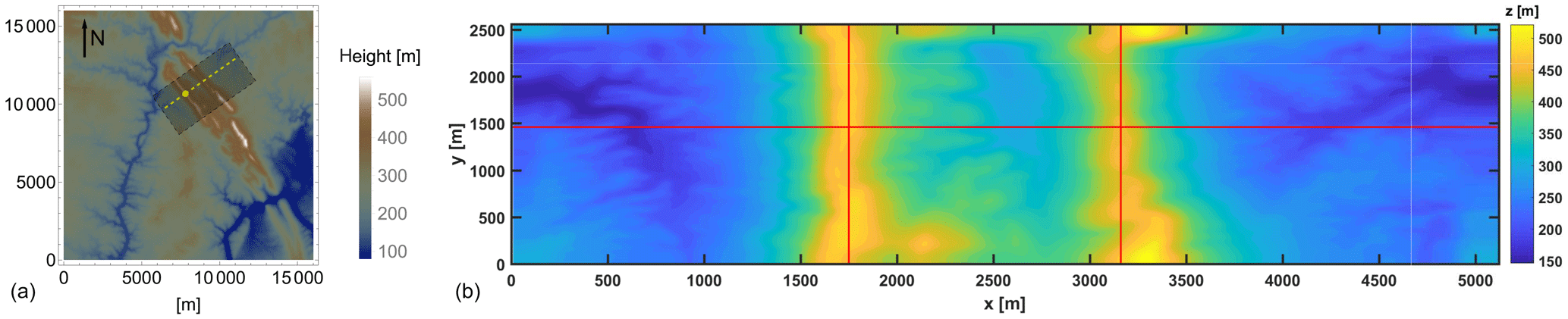
Figure 1 Terrain elevation variation at Perdigão. (a) Shaded rectangle represents the simulated area, with a yellow line passing through the main transect of the turbine location (source: Berg et al., 2017); (b) shaded region from (a) with intersection of red lines representing the turbine locations.

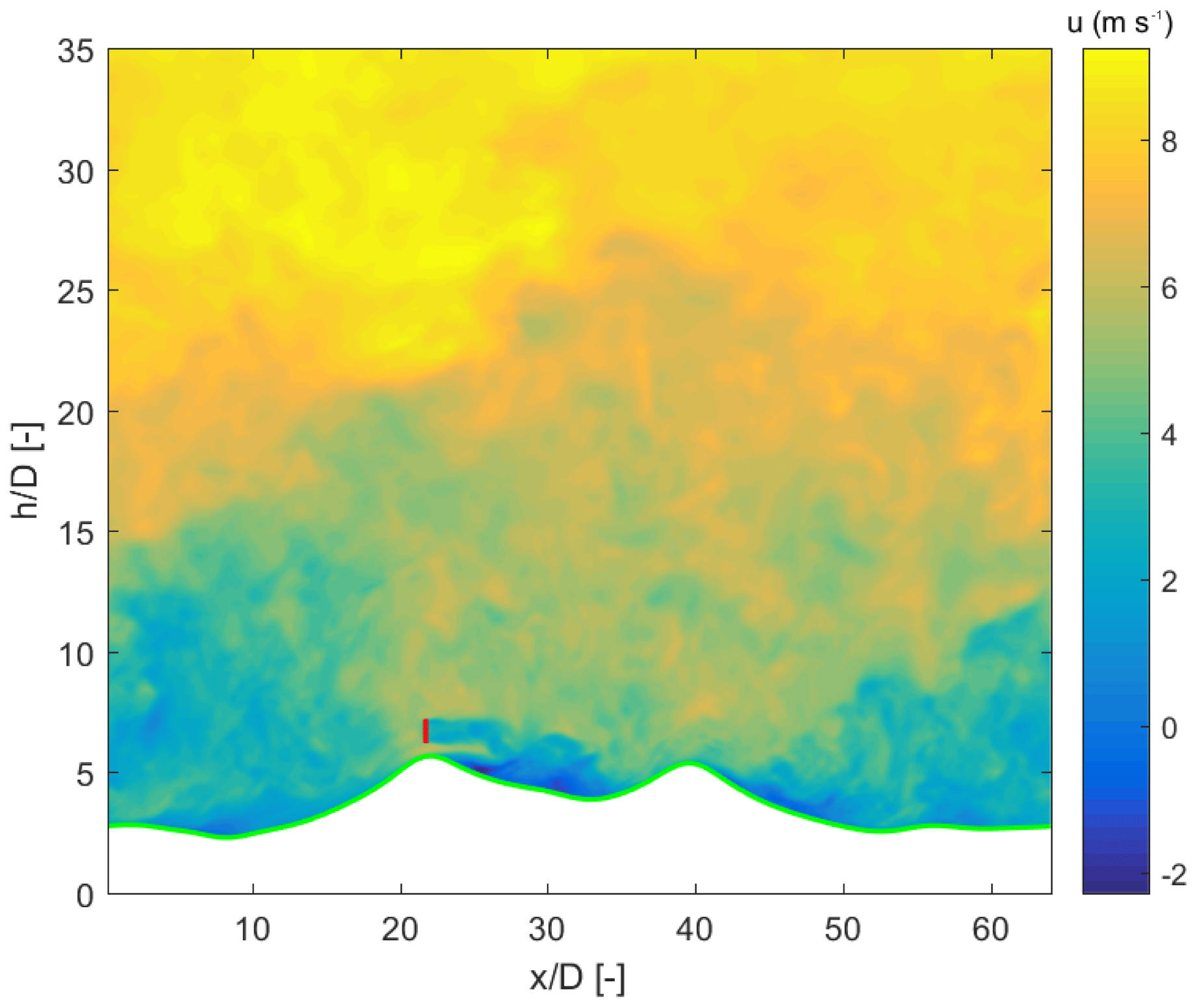
Figure 2 Instantaneous velocity in the streamwise direction along the main transect with turbine (in red).

The iteration procedure performed when solving the Poisson equation is expensive due to the strong coupling between pressure and vertical wind component and the fact that, in contrast to flat terrain, pressure gradients are quite high in complex terrains and thus require more time to fully converge. Slight smoothing of the terrain can help in reducing the computation time by reducing the number of pressure iterations required to attain convergence. This is done by applying an exponential filter in the wave number (x and y) space. This filtering process is given as follows:

$$\begin{array}{}\text{(14)}& \begin{array}{rl}{h}^{\mathrm{model}}(x,y)=& \int \int h^{\mathrm{true}}\left(k_x,k_y\right)\stackrel{\mathrm{̃}}{F}\left(k_x,k_y\right)\\ & e^{i\left(k_{x}x+k_{y}y\right)}\mathrm{d}{k}_x\mathrm{d}{k}_y,\end{array}\end{array}$$

where $\stackrel{\mathrm{̃}}{F}(k_x$, k_y) is the exponential filter given by

$$\begin{array}{}\text{(15)}& \stackrel{\mathrm{̃}}{F}\left(k_x,k_y\right)=e^{-\mathit{\alpha }\left[{\left(k_x\mathrm{\Delta }x\right)}^{\mathrm{2}}+{\left(k_y\mathrm{\Delta }y\right)}^{\mathrm{2}}\right]}.\end{array}$$

Here, α is the control parameter which determines the level of smoothing. Two different values of α used in the current study are 4 and 0.5, which result in maximum terrain slopes of 0.57 and 0.77 across the main transect, respectively. The steep terrain nearly matches the original terrain. The α value of 0.5 instead of 0 is chosen for this terrain to avoid the Gibbs phenomenon. Figure 3 shows a comparison of two terrains at a fixed lateral position passing through the turbine location. From here onward, a terrain with maximum slope of 0.57 will be referred to as “smooth”, whereas one with maximum slope of 0.77 will be referred to as “steep”.

Figure 3 Comparison of terrains with two different slopes along the main transect.

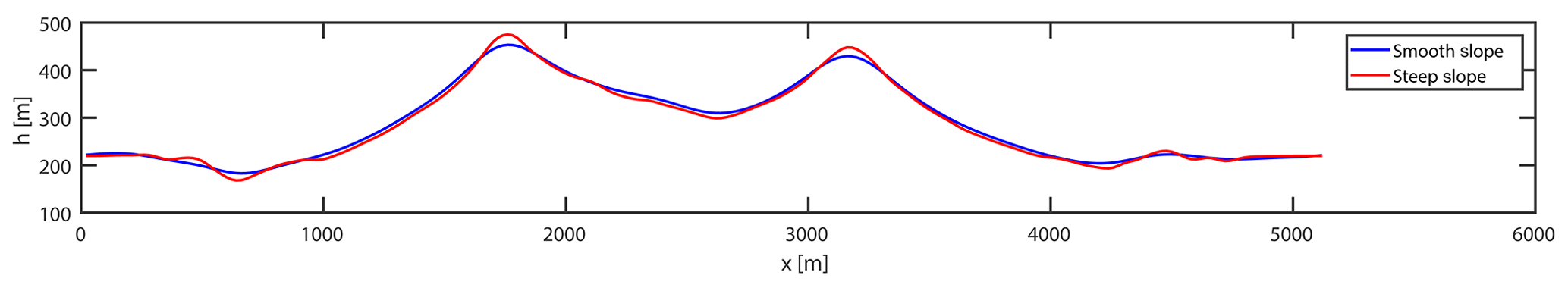
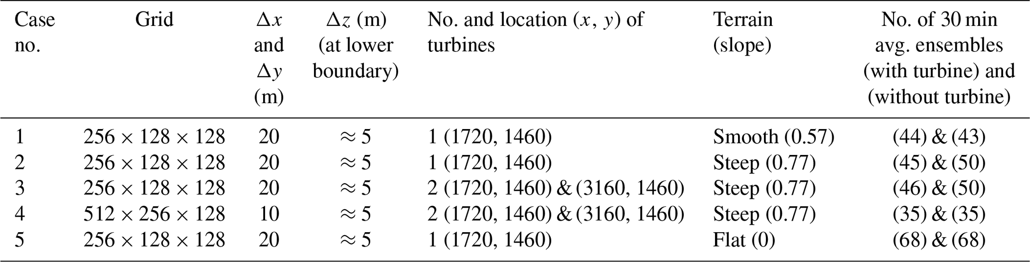
Table 1 gives an overview of various cases analyzed in the current study. It is to be noted that the number of ensembles used is fairly high to guarantee stationarity and an apparent difference in the number of ensembles for different cases does not affect the results. The aspect ratio of 1:4 in the case of 20 m resolution lies toward the limit of the allowed aspect ratio for the chosen subgrid scale model (rule of thumb).

Table 1 Description of cases analyzed in the study.

3.1 Boundary conditions

The boundaries in the horizontal directions are fully periodic, where a constant pressure gradient given by dP∕d$x=-u_{*}^{+\mathrm{2}}/H$ is applied in the x direction to drive the flow. Here, $u_{*}^{+}$ is the friction velocity chosen to be 0.6 m s⁻¹ and H is the height of domain equal to 3000 m. It is worth mentioning here that due to complexity of the terrain, the value used for friction velocity is not the effective friction velocity in the domain (discussed later). The periodicity in the horizontal directions means that the terrain is repeating itself, i.e., the inflow is affected by the terrain in the domain itself. We have made tests with extended buffer regions (not shown) which indicated that the turbulence level in the incoming flow was not affected by the terrain itself, and we therefore do not consider the periodicity to be a shortcoming of the later conclusions.

The lower surface of the domain is modeled assuming a log-law behavior in the first cell as a pointwise implementation (Bou-Zeid et al., 2004). A no-stress condition is applied at the upper boundary of the domain. Under this condition, the gradients of horizontal velocity components are set to zero, and the vertical velocity component itself is set to zero. Moreover, the subgrid scale energy (e) is also set to zero at upper boundary.

3.2 Data description

We base our analysis on averaged LES data, a choice associated with the need of stationary flow characteristics required for evaluation of self-similar wake statistics. We save 30 min averaged LES fields and by averaging a number of these fields together a total time necessary to guarantee stationarity is obtained. The rule for this averaging is defined as follows:

$$\begin{array}{}\text{(16)}& \langle u\rangle ={\displaystyle \frac{\mathrm{1}}{N}}\sum _{n=\mathrm{1}}^N{u}_{(\mathrm{30},n)},\end{array}$$

where 〈u〉 is the three-dimensional ensemble averaged velocity field, u_(30,n) is the nth 30 min averaged field and N is the total number of 30 min averages used, as given in Table 1 for each case. To simplify the notations, mean streamwise velocity computed using the above rule will be denoted by u=〈u〉.

4 Wake flow nomenclature

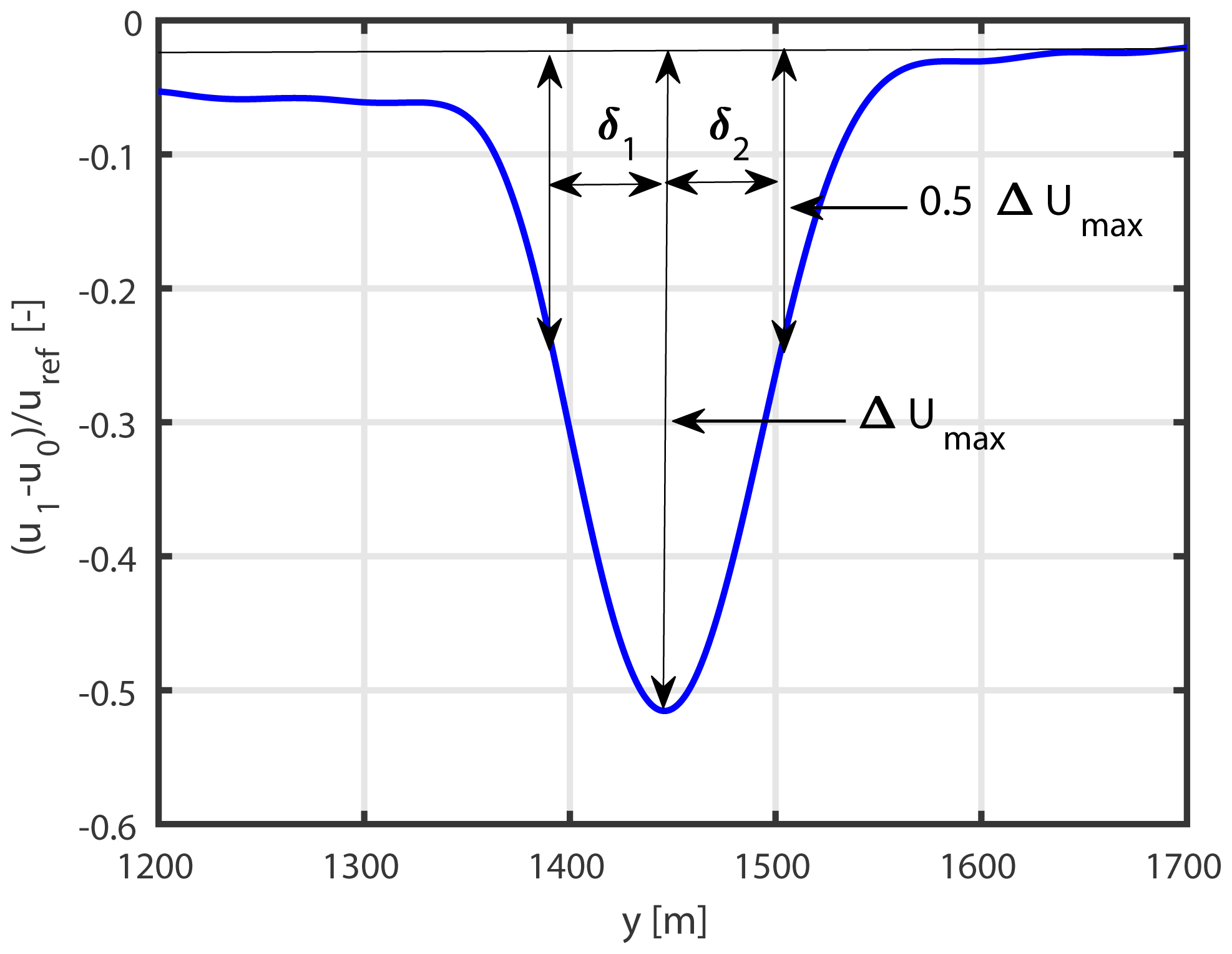
The quantities required to characterize the wake flow for the self-similarity check are defined in the current section. We first define the normalized mean velocity deficit as follows:

$$\begin{array}{}\text{(17)}& \mathrm{\Delta }U={\displaystyle \frac{u_{\mathrm{1}}-u_{\mathrm{0}}}{u_{\mathrm{ref}}}},\end{array}$$

where u₁ is the averaged streamwise velocity in the simulation including the turbine and u₀ is the same in the absence of the turbine. The mean difference is then normalized with a reference velocity, which corresponds to the velocity at the hub height of the first turbine in the absence of the turbine. Table 2 lists the reference velocities used for different cases.

Table 2 Reference velocities at hub height used for different cases.

Wake half-width is defined as the distance from wake center to the point where the velocity deficit is reduced to 50 % of the maximum velocity deficit. As wind turbine wakes can be asymmetric, the wake half-width is computed for two sides of the wake individually. The nomenclature used when describing the wake characteristics is defined in Fig. 4. The wake centerline is traced by identifying the point of maximum velocity deficit at each downstream location.

Figure 4 Nomenclature for wake half-width.

5 Results

5.1 Inflow velocity

To characterize the incoming flow velocity, normalized mean velocity profiles at 20 rotor diameters (20 D) upstream of the first ridge for different cases along with a logarithmic profile are shown in Fig. 5. Here, u_h refers to the velocity at the hub height approximately 20 rotor diameters upstream in the streamwise direction. It can be observed that the simulated velocity profiles show some deviation from the logarithmic profile, especially in the case of complex terrain. These deviations are somewhat expected, as the logarithmic profile is not completely valid in heterogeneous terrains. Moreover, the deviations observed are due to differences in the slopes of various profiles, whereas the quantitative values lie very close to the logarithmic profile. The periodic boundary conditions also play a role in determining the inflow velocity and therefore could be responsible for some of the deviations from the logarithmic profile.

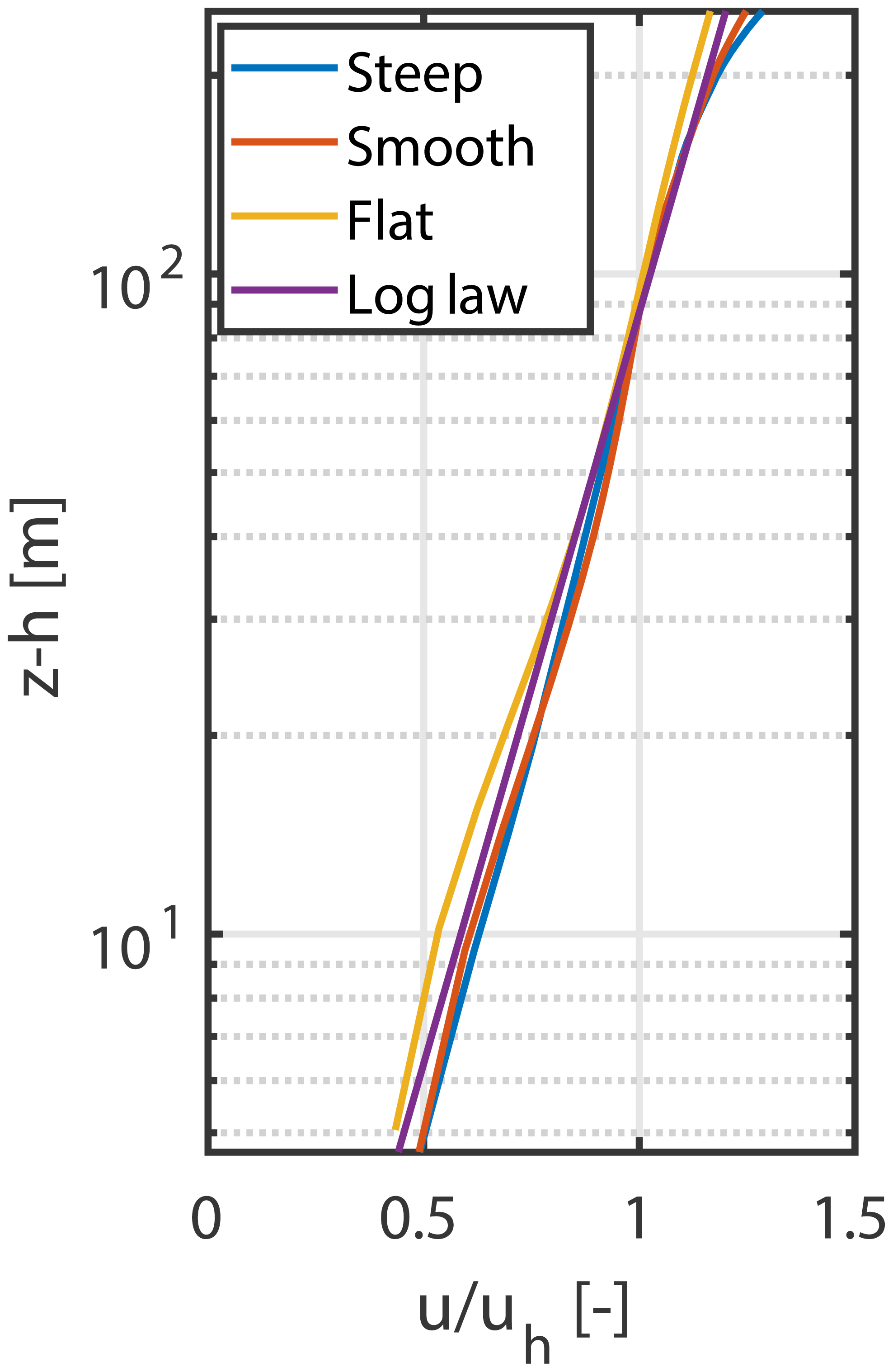
Figure 5 Comparison of normalized mean streamwise velocity at x=20 m. Smooth and flat cases have a resolution of 20 m, whereas the steep case has a resolution of 10 m.

5.2 Impact of grid resolution

The steep slope case is simulated at two different horizontal grid resolutions of 20 and 10 m. It should be mentioned that our procedure includes contributions from two effects: the grid resolution itself but also terrain effects, since more terrain is resolved in the 10 m case compared to the 20 m case. Figure 6 shows vertical profiles of streamwise velocity across the turbine located on top of the first ridge for the two grid resolutions. Comparing the velocity profiles in the two cases, good agreement is observed at respective downstream locations. However, it is important to note that the agreement between velocity profiles for the two cases is sensitive to the chosen reference velocity. Figure 7 shows a comparison of streamwise velocity along the main transect at the hub height, as well as local slopes, for the two grid resolutions. Whereas the qualitative trend of the velocity profiles matches well for the two resolutions, the quantitative values differ by up to 15 % between the two cases. This apparent discrepancy can be somewhat justified by the change in terrain characteristics caused by the change in resolution. As the resolution gets finer, the terrain becomes more detailed and the slopes are slightly changed. This can be verified by comparing the relative vertical distance between local surface and rotor positions up- and downstream of the ridge.

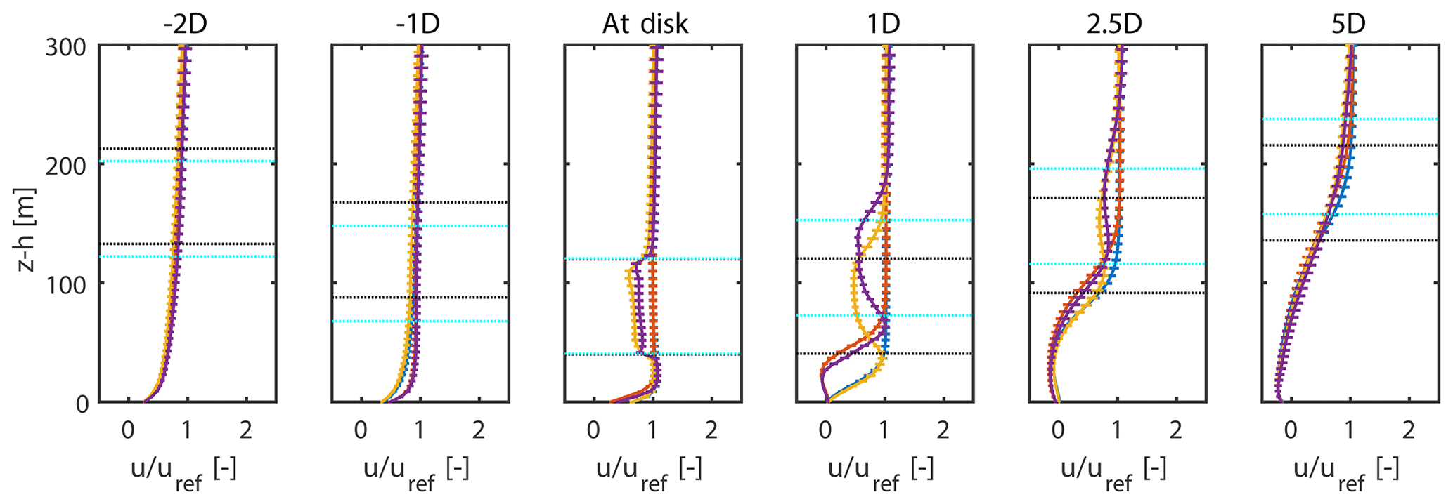
Figure 6 Vertical profiles of normalized mean streamwise velocity around first ridge for two different grid resolutions. Blue and yellow vertical lines show velocity profiles without and with turbine for 20 m resolution, whereas red and purple vertical lines show profiles without and with turbine for 10 m resolution. Black horizontal lines trace rotor top and bottom for the coarse grid resolution, whereas cyan horizontal lines trace the same for finer-grid resolution. The error bars correspond to $\mathit{\sigma }/\sqrt{N}$, where σ is the standard deviation and N is the number of 30 min ensembles used.

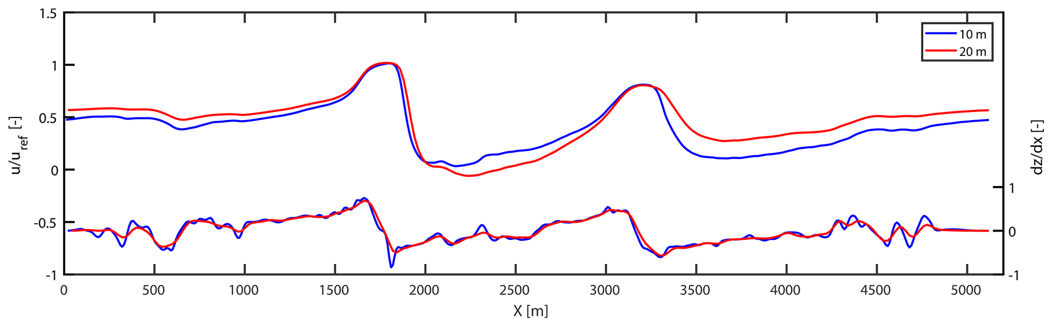
Figure 7 Comparison of streamwise velocity at the hub height without turbine and local slopes along the main transect for the two grid resolutions.

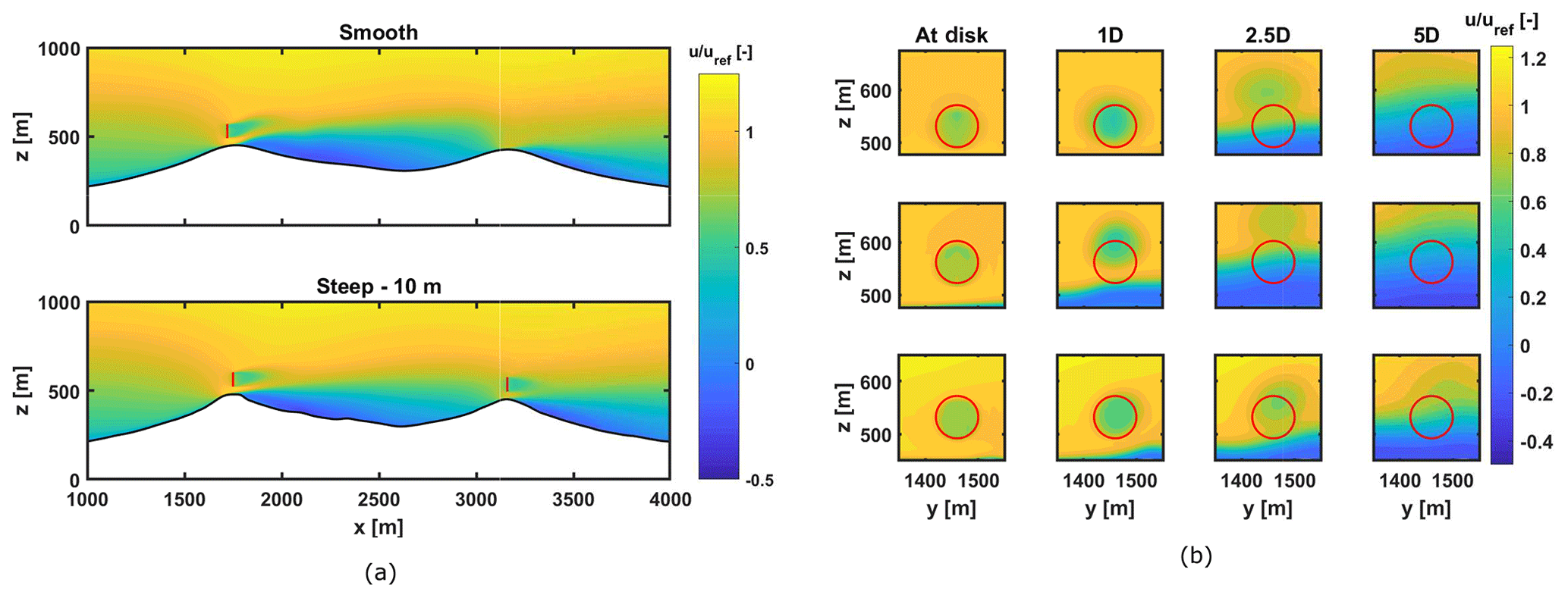
Figure 8 (a) Streamwise velocity profile for smooth and steep terrain; (b) wake development in the rotor plane at different downstream locations. First row: first turbine, smooth terrain – 20 m resolution; second row: first turbine, steep terrain – 10 m resolution; third row: second turbine, steep terrain – 10 m resolution. Rotor position is highlighted by the red circle.

Recall that in Sect. 3.1 the flow was defined to be pressure-gradient-driven with a friction velocity of 0.6 m s⁻¹. This balance between pressure gradient and friction velocity would hold true in flat terrain, whereas in complex terrain there is an additional contribution from the form drag generated by the two ridges. The immediate impact of this additional contribution is a reduced friction velocity in the terrain. As the terrain gets more detailed in the finer grid, the friction velocity is further decreased by virtue of an increased contribution from form drag. We believe that this difference in friction velocity in the two grid resolutions can explain the difference in the velocity profiles observed here.

A comparison of the LES flow characteristics in different terrains and resolutions with field measurements, although without any turbine in the terrain, was recently presented by Berg et al. (2018). Good agreement between the measurements and simulations was obtained, keeping in mind the simple flow conditions defined in the simulations.

Figure 9 Lateral profiles of streamwise velocity deficit for different cases.

Figure 10 Vertical profiles of streamwise velocity deficit for different cases.

5.3 Wake characteristics

A fundamental question can be formulated around the interaction of wake from the turbine with the local terrain. Understanding this kind of interaction is important in order to know how the wake behaves within a complex terrain and how the terrain-generated phenomena impact the behavior of the rotor wake. Figure 8a shows the wakes from turbines in two different terrains and two different locations (top of the respective ridges). An important impact of local topography on wakes is the change in the orientation of wakes behind the two turbines. The strong recirculation regions developed behind the ridges due to flow separation generate their own shear layers, which do not allow the turbine wakes to mix with them. It is for this reason that we observe an upward orientation for the turbines located on top of the first ridge in the two cases. For the smooth terrain, the recirculation starts on top of the ridge and the height of this region extends higher than the ridge top. This causes an initially horizontal wake to shift in an upward direction. For the steep case, however, the high slopes result in an upward inclination of the wake from the rotor position. For the turbine located on the second ridge, the wake is oriented in a slightly downward, somewhat terrain-following, orientation. This is due to the fact that the recirculation region behind the second ridge is smaller than the ridge top and thus allows the wake to move in a downward direction.

Figure 8b shows wake development in the rotor plane. The sideways movement of wake can be observed in the three cases, as the wake moves downstream. Although the most probable reason for this sideways movement is the terrain complexity and variation in pressure distributions across the terrain, any conclusive statement cannot be made due to the limitations of grid resolution employed in the current study.

An important feature of the wake is the relatively faster recovery as compared to the flat terrain. High levels of turbulent mixing in the atmosphere due to complexity of the terrain provide a catalyst effect and thus promote quick recovery of the wake. It is thereby observed that the wake is almost recovered at a distance of around 5 rotor diameters in the downstream. This faster wake recovery in the complex terrain has been previously reported by various other studies (Politis et al., 2012; Astolfi et al., 2018; Tabib et al., 2016).

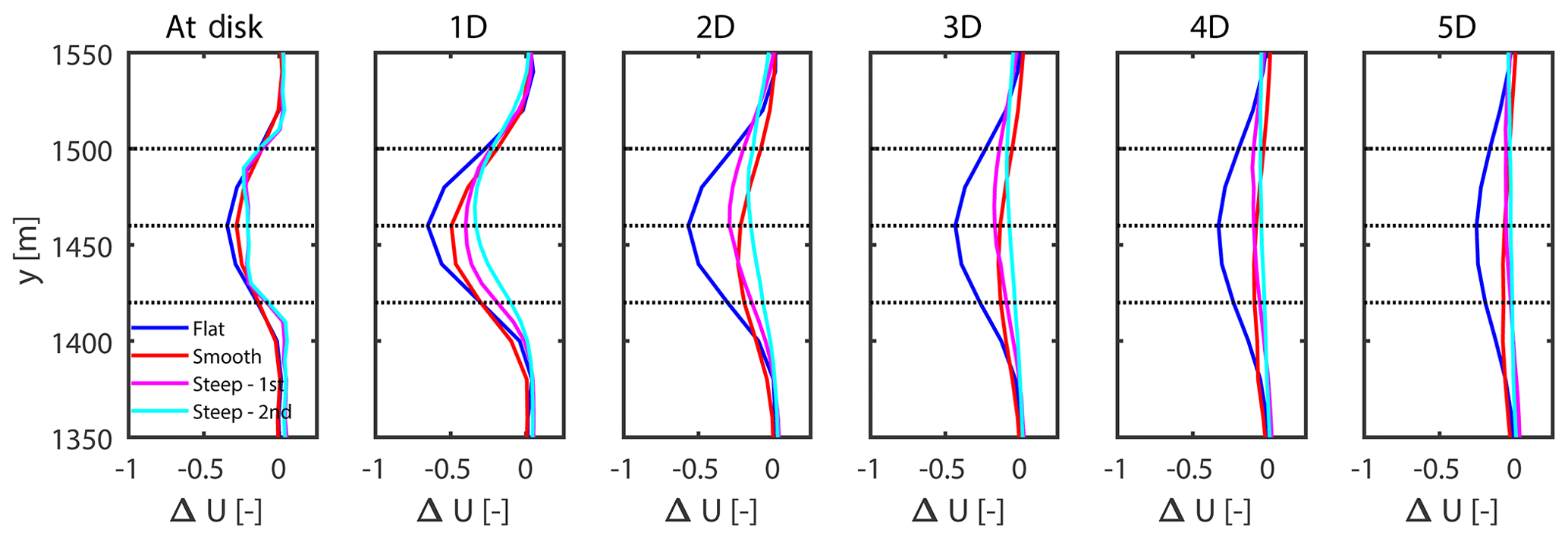
Velocity deficit profiles

Figures 9 and 10 show normalized mean velocity deficit profiles for different cases (flat, smooth, steep – 10 m and first turbine; steep – 10 m and second turbine) at different downstream locations. Comparing the lateral profiles, it is observed that the finer-grid resolution in the lateral direction captures the wake structure much better than the coarser resolutions. Moreover, the velocity deficit decays at a much slower rate in the flat case than the other (complex) cases. The velocity deficit for the turbine located on the second ridge is observed to be the smallest with the fastest recovery. This can be attributed to the highest ambient turbulence in the wake of the particular turbine among the considered cases. To support this argument, we plot normalized profiles of turbulent kinetic energy, TKE = $\frac{\langle {\mathit{\sigma }}_u^{\mathrm{2}}+{\mathit{\sigma }}_v^{\mathrm{2}}+{\mathit{\sigma }}_w^{\mathrm{2}}\rangle }{\mathrm{2}}$ (see Fig. 11). As turbulent kinetic energy is responsible for transport of energy in the domain, it can be used to quantify the wake recovery. From the figure it is clearly observed that the turbulent kinetic energy for complex terrain cases is significantly higher than the flat terrain case. The turbine located on top of the second ridge in the steep case shows the highest levels of TKE, thus causing fastest wake recovery.

Figure 11 Vertical profiles of normalized turbulent kinetic energy for different cases.

5.4 Wake self-similarity

Figure 12 shows how the maximum velocity deficit develops as the wake moves in the downstream. An increasing–decreasing behavior can be observed, with the smooth case showing the highest velocity deficit. At a downstream distance of 5 rotor diameters, the three complex cases show very close numbers for maximum velocity deficit. The flat case (as expected) shows slowest recovery in wake.

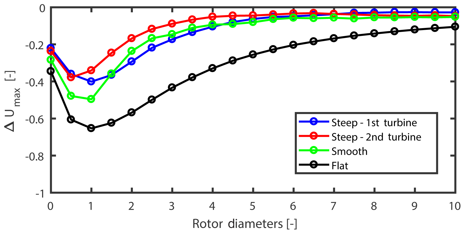
Figure 12 Maximum normalized mean velocity deficit as a function of downstream distance for different cases.

To further characterize the wake, we plot right and left wake half-widths for the lateral and vertical profiles in Fig. 13. The wake half-widths generally show an increasing trend with the downstream distance. For the lateral profiles the values are much closer near the turbine location and spread differently for different cases, whereas for vertical profiles the values have a wider spread due to varying levels of shear. The flat terrain is observed to have the smallest wake half-widths, whereas the second turbine in steep slope shows highest values. This can be attributed to the rate of wake recovery in the respective cases. Finally, the difference in the left and right wake widths for a specific location highlights the wake symmetry or asymmetry.

Figure 13 Right and left wake half-width for the (a) lateral and (b) vertical velocity deficit profiles.

We now plot normalized velocity deficit profiles against normalized distance from wake center. The velocity deficit profiles are normalized with the maximum velocity deficit for the respective profiles, whereas the centered distance is normalized with wake half-width on either side of the wake center.

Figure 14a shows lateral self-similar velocity deficit profiles for the flat case. The profiles follow the Gaussian profile and last from a downstream distance of 1 to 9 rotor diameters. The same profiles for three complex cases shown in Fig. 14b also collapse on the Gaussian profile; however, two important things should be noted. First the self-similarity holds for a much shorter distance (from 1 to 3 rotor diameters). This can be attributed to the faster wake recovery in complex cases and to the fact that the localized terrain changes disrupt the wake structure and thus deviations from self-similarity occur. The second important feature is the wide spread in the tails of the profiles for three complex cases. Whereas the profiles for a single case (denoted by same color) are much closer to each other, wider spread is seen while comparing profiles for two different cases. This can be due to the difference in the shear toward the edges of the wakes in different cases and to the differences arising due to differences in terrains, flow separation characteristics and levels of turbulence. Now, Fig. 14b shows velocity deficit profiles extracted from a horizontal plane passing through the hub height of the respective turbine; however, from Fig. 8, we observe significant deflection in the vertical direction. In order to account for this wake deflection, we track the maximum velocity deficit point in the vertical direction at each downstream location and extract the corresponding lateral velocity profiles. Figure 15 shows the resulting self-similar profiles of streamwise velocity deficit from 1 to 6 D. Computing self-similar profiles beyond 6 D is not possible, as the wake is almost recovered (the max velocity deficit drops below 0.04 for >6 D). Comparing with Fig. 14b, the profiles are observed to be self-similar for a longer distance; however, beyond 3.5 D, the left-side tail of the profiles depart from the Gaussian profile with increasing downstream distance.

Figure 14 Self-similar lateral profiles of streamwise velocity deficit (a) flat case (b) complex cases for a downstream distance of 1 D to 3 D with intervals of 0.5 D; inset shows normalized velocity deficit profiles from 3.5 D to 5 D.

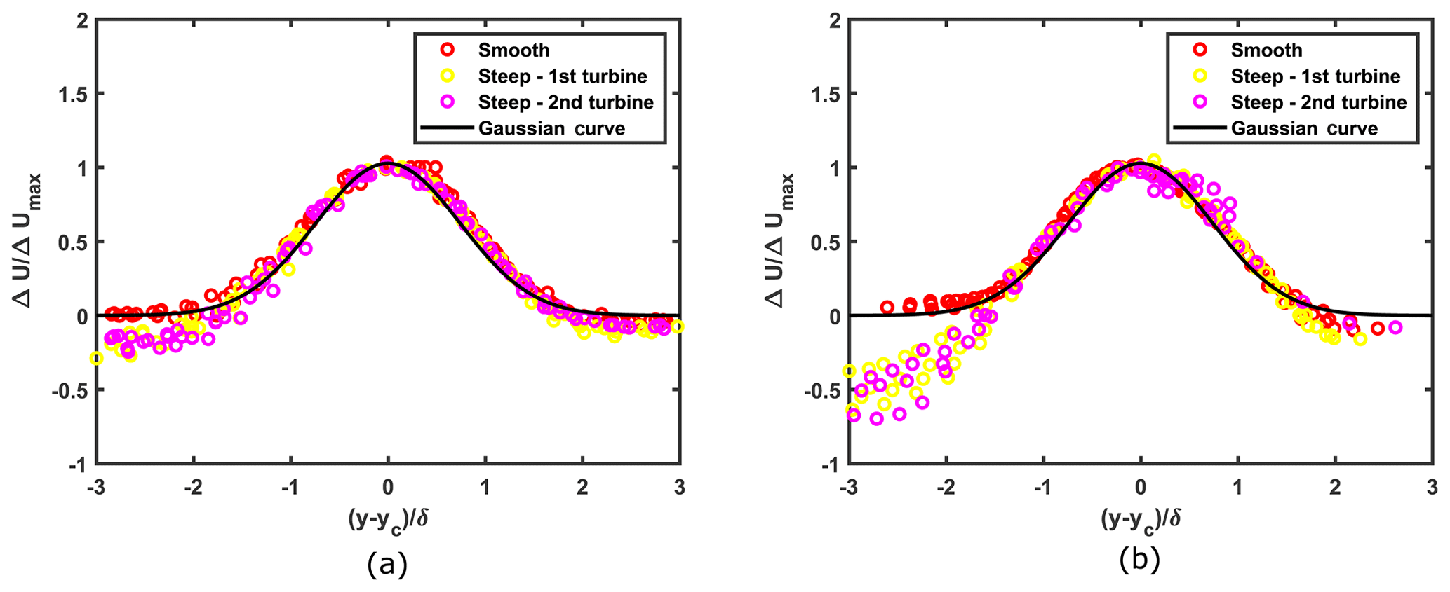
Figure 15 Self-similar lateral profiles of streamwise velocity deficit for complex cases accounting for wake deflection in the vertical direction for a downstream distance of (a) 1 D to 3.5 D and (b) 4 D to 6 D.

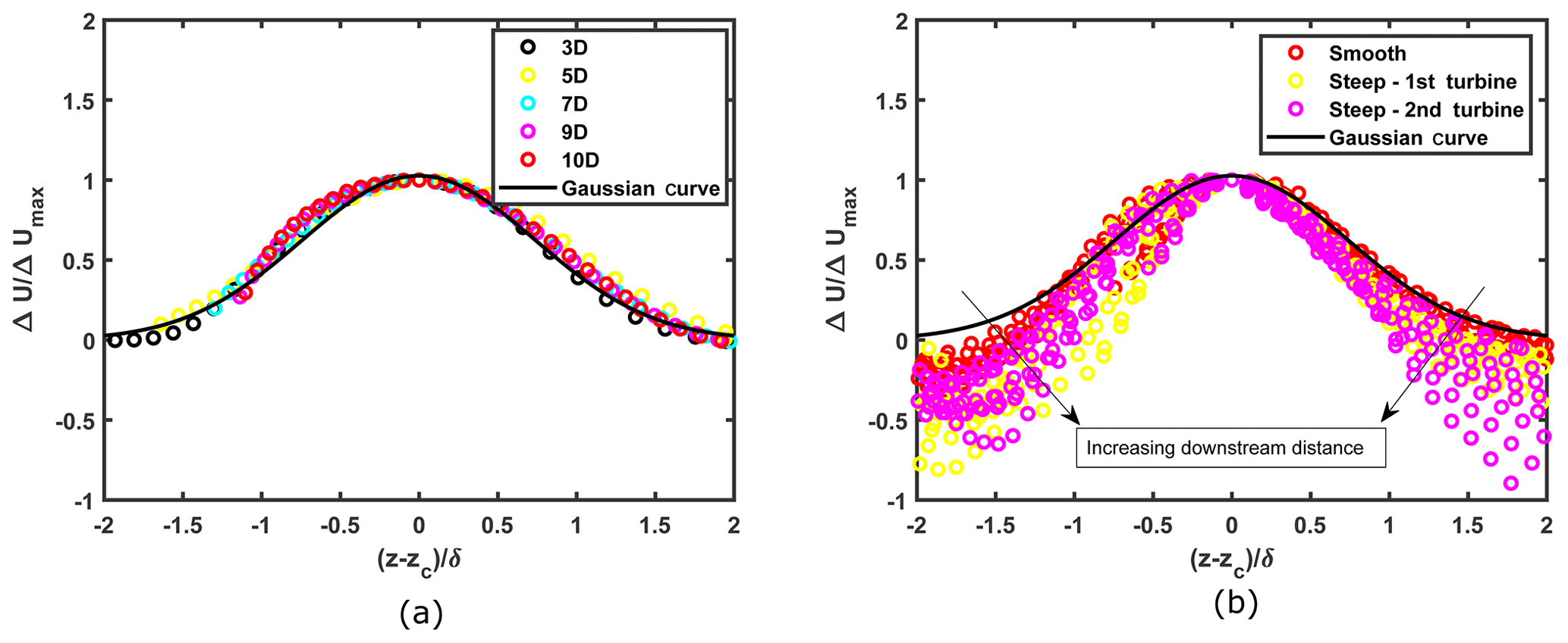
Figure 16 Self-similar vertical velocity deficit profiles (a) flat case (b) complex cases for a downstream distance of 1 D to 5 D with intervals of 0.5 D. Arrows indicate direction of increasing downstream distance.

Figure 16a shows vertical self-similar velocity deficit profiles for the flat case. Self-similarity is observed from a distance of 3 to 10 rotor diameters. In the complex cases (Fig. 16b), self-similarity in the vertical profiles is observed from 1 to 3 rotor diameters. As indicated by arrows in Fig. 16b, the spread in tails of profiles increases with increasing downstream distance. Beyond 3 D, this spread is significantly high. These profiles also show a much wider spread when compared to the lateral profiles. Moreover, they exhibit more asymmetric behavior than the lateral profiles. This is due to the impact of surface and vertical wind shear. In addition, as the terrain is complex, varying levels of slope lead to varying distances between the projected rotor area and the surface, which eventually gives rise to high variation among profiles at different downstream locations.

6 Conclusion

Terrain-generated phenomena can have a significant impact on the wake characteristics of a turbine located in a complex terrain. In this study, we attempted to verify whether the self-similarity, which is one the fundamental characteristics of wakes, still holds in complex terrains or not. In this context, we performed large eddy simulation of wind turbine(s) located in a flat and complex terrain. By varying turbine location, as well as terrain complexity, we simulated different flow scenarios in complex terrain. By plotting normalized velocity deficit profiles in the lateral, as well as vertical, direction, we looked for self-similarity in the simulated cases. We observed that wakes in complex terrain preserve self-similarity in both directions. The region of this preservation is, however, over much shorter distances downstream than the flat terrain counterpart. This is attributed to the deformation of wakes in the far wake region by varying heights of the terrain and to the faster wake recovery in the complex terrain. Finally, vertical profiles show a wider spread and higher asymmetry than the lateral ones.