Augmented Kalman filter with a reduced mechanical model to estimate tower loads on a land-based wind turbine: a step towards digital-twin simulations

This article presents an application of the Kalman filtering technique to estimate loads on a wind turbine. The approach combines a mechanical model and a set of measurements to estimate signals that are not available in the measurements, such as wind speed, thrust, tower position, and tower loads. The model is severalfold faster than real time and is intended to be run online, for instance, to evaluate real-time fatigue life consumption of a field turbine using a digital twin, perform condition monitoring, or assess loads for dedicated control strategies. The mechanical model is built using a Rayleigh–Ritz approach and a set of joint coordinates. We present a general method and illustrate it using a 2-degrees-of-freedom (DOF) model of a wind turbine and using rotor speed, generator torque, pitch, and tower-top acceleration as measurement signals. The different components of the model are tested individually. The overall method is evaluated by computing the errors in estimated tower-bottom-equivalent moment from a set of simulations. From this preliminary study, it appears that the tower-bottom-equivalent moment is obtained with about 10 % accuracy. The limitation of the model and the required steps forward are discussed.

1 Introduction

Wind turbines are designed and optimized for a given site or class definition using both numerical tools and a statistical assessment of the environmental conditions the turbine will experience. The uncertainty of the tools and data is accounted for using multiplicative safety factors that are determined from a combination of experience and specifications by the standards. Overconservative safety factors will imply unnecessary costs that may be alleviated later on by extending the lifetime of a project. An underestimate of the safety factor will likely lead to catastrophic failures. Once a design is complete and the product is in place, is it possible to predict what the lifetime of the wind turbine will be.

Digital twins are becoming increasingly popular to follow the life cycle of a physical system. This concept is used to bridge the gap between the modeling and measurement realm: real-time measurements from the physical system are communicated to a digital system, and this information is combined with a numerical model to estimate the state of the system and potentially predict its evolution. A Kalman filter is one example of a technique that can be used: it combines a model of a system with a set of measurements on that system to predict additional variables, such as positions or loads at points where no measurements are available. In this study, we focus on Kalman filter methods, but other load estimation techniques may be used, such as lookup tables (Mendez Reyes et al., 2019), modal expansion (Iliopoulos et al., 2016), machine learning (Evans et al., 2018), neural networks (Schröder et al., 2018), polynomial chaos expansion (Dimitrov et al., 2018), deconvolution (Jacquelin et al., 2003), or load extrapolation (Ziegler et al., 2017).

Kalman filters have been extensively used in control engineering with a wide range of applications. Auger et al. (2013) provide a review of some industrial applications. Load estimations using Kalman filtering are found, for example, in the following references: Ma and Ho (2004) and Eftekhar Azam et al. (2015). In the context of wind energy, wind speed estimation is critical for the determination of the dynamics of the system. This topic was investigated using parametric models by Bozkurt et al. (2014); using Kalman filters by Østergaard et al. (2007), Knudsen et al. (2011), and Song et al. (2017); and using Luenberger-type observers by Hafidi and Chauvin (2012). A comparison of wind speed estimation technique is found in Soltani et al. (2013). The techniques were extended to also estimate the wind shear and turbine misalignments; see, for example, Bottasso et al. (2010), Simley and Pao (2016), and Bertelè et al. (2018). Kalman filtering has been used to estimate rotor loads and wind speed in application to rotor controls by Boukhezzar and Siguerdidjane (2011). General approaches use Kalman filtering in combination with a model of the full wind turbine dynamics. These approaches were used for wind speed estimation and load alleviation via individual pitch control (Selvam et al., 2009; Bottasso and Croce, 2009) and for online estimation of mechanical loads (Bossanyi, 2003). An example of estimating tower loads with the acceleration sensor is found in Hau (2008). Bossanyi et al. (2012) compared the observed rotor and tower loads with measurements and investigated the potential of the control method to reduce damage-equivalent loads.

The methodology presented in this article uses an augmented Kalman filter (Lourens et al., 2012) to estimate loads on the wind turbine based on measurement signals commonly available in the nacelle. The method builds on the approach used by Bossanyi et al. (2012) and Lourens et al. (2012). The method of Lourens et al. (2012) is generalized. On the other hand, the expression of the mechanical system may be seen as simplified compared to the approach of Bossanyi et al. (2012): a Rayleigh–Ritz formulation is used, and the system is not further linearized. The equations are given in full for a 2-degrees-of-freedom (DOF) system, and the source code is made available online. The time series of estimated loads are applied to assess the fatigue life consumption of the turbine components using the rainflow-counting method. The study focuses on the determination of tower loads of land-based wind turbines, but other signals may be extracted from the estimated states, such as the tower-top displacement, the aerodynamic loads, and the wind speed. A scheme of the method is provided in Fig. 1.

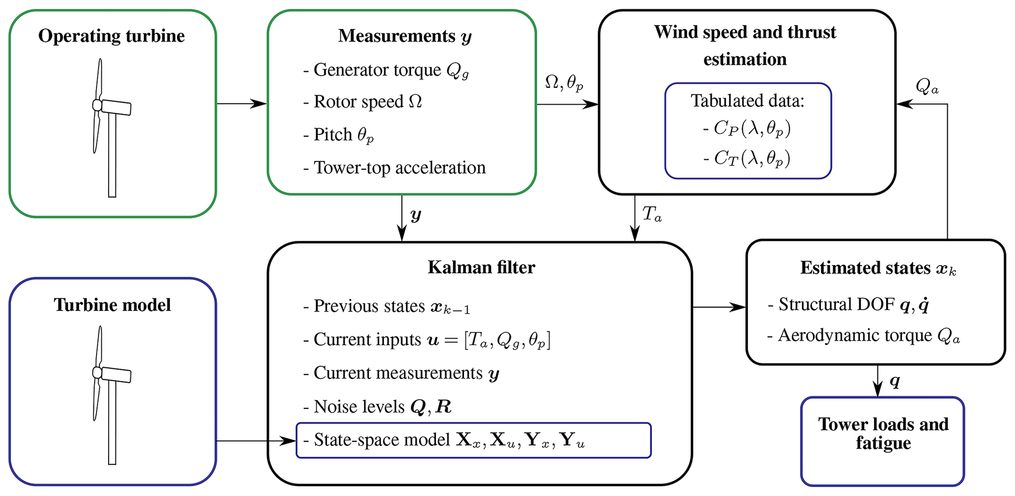
Figure 1 Main components of the model: wind turbine measurements and a turbine model are combined to estimate tower loads. A wind speed estimator and a Kalman filter algorithm are used in the estimation. Turbine model dependencies are framed in blue.

The numerical model of the wind turbine relies on a Rayleigh–Ritz shape-function approach with reduced numbers of DOFs (Branlard, 2019a). The wind speed is estimated using an approach similar to Østergaard et al. (2007), and the thrust force estimation is based on this wind speed estimate. The generator torque, rotor speed, and tower-top accelerations are used as measurements and combined with the numerical model within an augmented Kalman filter. The time series of loads in the tower are determined based on the tower shape function and the tower degrees of freedom, and the fatigue loads are computed from this signal. It is noted that the method is expected to be more accurate at the tower bottom than the tower top because rotor asymmetric loading cannot be captured from the single acceleration measurement. This limitation can be overcome by including more measurement channels and states. Possible improvements of the method are mentioned in the discussion section of this article.

Section 2 presents the different components required for this work: the augmented Kalman filter; the numerical model of the turbine; and the estimators for the wind speed, thrust, tower load, and fatigue. Simple illustrations and validation results for the different components of the model are provided in Sect. 3. Section 4 presents full applications but is limited to simulations. Discussions and conclusions follow.

2 Description of the models

2.1 Example for a 2-DOF wind turbine model

We start this section with an illustrative example before describing the different parts of the model in their general form. A wind turbine is modeled here using 2 DOFs: (1) the generalized coordinate associated with the fore–aft bending of the tower, q_t, and (2) the shaft rotation, ψ. The tower bending is associated with a shape function, Φ_t(z), such that the fore–aft displacement of a point at height z and at time t is given by $u(z,t)=q_{\mathrm{t}}\left(t\right){\mathrm{\Phi }}_{\mathrm{t}}\left(z\right)$. The shape function is normalized to unity at the tower top, and q_t is then equal to fore–aft displacement at the tower top (see Fig. 2). The equations of motion of the system are

$$\begin{array}{}\text{(1)}& \left[\begin{array}{cc}M& \mathrm{0}\\ \mathrm{0}& J\end{array}\right]\left[\begin{array}{c}{\ddot{q}}_{\mathrm{t}}\\ \ddot{\mathit{\psi }}\end{array}\right]+\left[\begin{array}{cc}C& \mathrm{0}\\ \mathrm{0}& \mathrm{0}\end{array}\right]\left[\begin{array}{c}{\dot{q}}_{\mathrm{t}}\\ \dot{\mathit{\psi }}\end{array}\right]+\left[\begin{array}{cc}K& \mathrm{0}\\ \mathrm{0}& \mathrm{0}\end{array}\right]\left[\begin{array}{c}{q}_{\mathrm{t}}\\ \mathit{\psi }\end{array}\right]=\left[\begin{array}{c}{T}_{\mathrm{a}}^{*}\\ Q_{\mathrm{a}}-Q_{\mathrm{g}}\end{array}\right],\end{array}$$

where M, C, and K are the generalized mass, damping, and stiffness, respectively, associated with the fore–aft DOF; J is the drivetrain inertia; $T_{\mathrm{a}}^{*}$ and Q_a are the aerodynamic thrust and torque, respectively; and Q_g is the generator torque. A superscript asterisk is used on the thrust to indicate that using the thrust directly is a rough approximation. A more elaborate expression of the generalized force acting on q_t is given in Sect. 3.3. The determination of M, C, and K is discussed in Branlard (2019a). For the National Renewable Energy Laboratory (NREL) 5 MW turbine, the values are $M=\mathrm{4.4}\times {\mathrm{10}}^{\mathrm{5}}$ kg, $D=\mathrm{2.5}\times {\mathrm{10}}^{\mathrm{4}}$ kg s⁻¹, $K=\mathrm{2.7}\times {\mathrm{10}}^{\mathrm{6}}$ kg s⁻², and $J=\mathrm{4.3}\times {\mathrm{10}}^{\mathrm{7}}$ kg m². We tuned the damping term C to account for aerodynamic damping, as mentioned in Sect. 3.3. Aerodynamic stiffness is included in $T_{\mathrm{a}}^{*}$. In this example, the system of equations is coupled only via the aerodynamic loads.

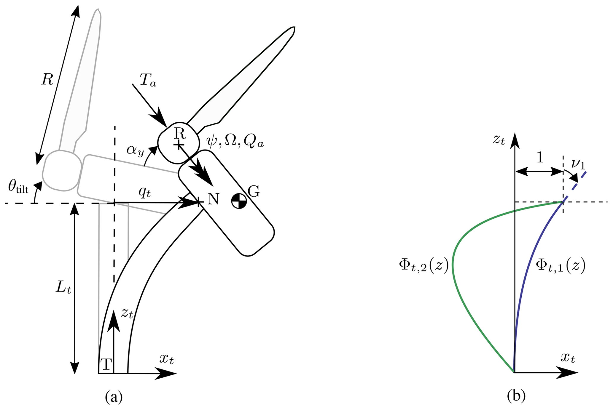
Figure 2 (a) Notations for the wind turbine model and (b) example of shape functions used for the tower. Definition of points: T is tower bottom; N is tower top; G is center of mass of the rotor nacelle assembly; R is rotor center. The shape functions are normalized to unity at point N. The slope at the extremity of the first shape function is written as ${\mathit{\nu }}_{\mathrm{1}}=\frac{\mathrm{d}{\mathrm{\Phi }}_{t,\mathrm{1}}}{\mathrm{d}z}\left(L_t\right)$.

The following measurements are usually readily available on any commercial wind turbine: the generator power, P_g; the blade pitch angle, θ_p; the rotor rotational speed, $\mathrm{\Omega }=\dot{\mathit{\psi }}$; and the tower-top acceleration in the fore–aft direction, ${\ddot{q}}_{\mathrm{t}}$. The knowledge of the generator power, speed, and losses allows for the estimation of the generator torque, Q_g. In this study, the generator torque is assumed to be known. We use an augmented Kalman filter concept to combine these measurements with the mechanical model to estimate the state of the system. The Kalman filter algorithm requires linear state and output equations. The state vector is assumed to be x=[q_t, ψ, ${\dot{q}}_{\mathrm{t}}$, $\dot{\mathit{\psi }}$, Q_a]. The fact that some of the loads were included into the state vector is referred to as “state augmentation”. The choice of loads to include in the state vector is not unique and will lead to different state equations. Using this choice for x, we write Eq. (1) into the following state equation:

$$\begin{array}{}\text{(2)}& \begin{array}{rl}\left[\begin{array}{c}{\dot{q}}_{\mathrm{t}}\\ \dot{\mathit{\psi }}\\ {\ddot{q}}_{\mathrm{t}}\\ \ddot{\mathit{\psi }}\\ {\dot{Q}}_{\mathrm{a}}\end{array}\right]& =\left[\begin{array}{ccccc}\mathrm{0}& \mathrm{0}& \mathrm{1}& \mathrm{0}& \mathrm{0}\\ \mathrm{0}& \mathrm{0}& \mathrm{0}& \mathrm{1}& \mathrm{0}\\ -M^{-\mathrm{1}}K& \mathrm{0}& -M^{-\mathrm{1}}C& \mathrm{0}& \mathrm{0}\\ \mathrm{0}& \mathrm{0}& \mathrm{0}& \mathrm{0}& J^{-\mathrm{1}}\\ \mathrm{0}& \mathrm{0}& \mathrm{0}& \mathrm{0}& \mathrm{0}\end{array}\right]\left[\begin{array}{c}{q}_{\mathrm{t}}\\ \mathit{\psi }\\ {\dot{q}}_{\mathrm{t}}\\ \dot{\mathit{\psi }}\\ Q_{\mathrm{a}}\end{array}\right]\\ & +\left[\begin{array}{ccc}\mathrm{0}& \mathrm{0}& \mathrm{0}\\ \mathrm{0}& \mathrm{0}& \mathrm{0}\\ M^{-\mathrm{1}}& \mathrm{0}& \mathrm{0}\\ \mathrm{0}& -J^{-\mathrm{1}}& \mathrm{0}\\ \mathrm{0}& \mathrm{0}& \mathrm{0}\end{array}\right]\left[\begin{array}{c}{T}_{\mathrm{a}}^{*}\left(\dot{\mathit{\psi }},Q_{\mathrm{a}},{\mathit{\theta }}_{\mathrm{p}}\right)\\ Q_{\mathrm{g}}\\ {\mathit{\theta }}_{\mathrm{p}}\end{array}\right],\end{array}\end{array}$$

where, for simplicity, the time derivatives of the aerodynamic torque are assumed to be zero, an assumption referred to as “random walk force model”. This assumption accounts for saying that the estimate of the torque at the next time step is likely to be close to the one at the current time step. Improvements on this is discussed in Sect. 5. The thrust is determined based on the rotor speed, aerodynamic torque, and pitch angle using tabulated data, as described in Sect. 2.4. The output equation relates the measurements to the states and inputs as follows:

$$\begin{array}{}\text{(3)}& \begin{array}{rl}\left[\begin{array}{c}{\ddot{q}}_{\mathrm{t}}\\ \dot{\mathit{\psi }}\\ Q_{\mathrm{g}}\\ {\mathit{\theta }}_{\mathrm{p}}\end{array}\right]& =\left[\begin{array}{ccccc}-M^{-\mathrm{1}}K& \mathrm{0}& -M^{-\mathrm{1}}C& \mathrm{0}& \mathrm{0}\\ \mathrm{0}& \mathrm{0}& \mathrm{0}& \mathrm{1}& \mathrm{0}\\ \mathrm{0}& \mathrm{0}& \mathrm{0}& \mathrm{0}& \mathrm{0}\\ \mathrm{0}& \mathrm{0}& \mathrm{0}& \mathrm{0}& \mathrm{0}\end{array}\right]\\ & \mathit{x}+\left[\begin{array}{ccc}{M}^{-\mathrm{1}}& \mathrm{0}& \mathrm{0}\\ \mathrm{0}& \mathrm{0}& \mathrm{0}\\ \mathrm{0}& \mathrm{1}& \mathrm{0}\\ \mathrm{0}& \mathrm{0}& \mathrm{1}\end{array}\right]\left[\begin{array}{c}{T}_{\mathrm{a}}^{*}\\ Q_{\mathrm{g}}\\ {\mathit{\theta }}_{\mathrm{p}}\end{array}\right].\end{array}\end{array}$$

Equations (2) and (3) are used within a Kalman filter algorithm to estimate the state's vector based on the measurements. The estimated time series of q_t, together with its associated shape function Φ_t, are used to determine the bending moments within the tower and estimate tower fatigue loads based on the method presented in Sect. 2.5. Results from this simple model is provided in Sect. 3. The rest of this section generalizes the approach presented.

2.2 Mechanical model of the wind turbine

The wind turbine is described using a set of DOFs that consist of joint coordinates and shape function coordinates. The method was described in previous work (Branlard, 2019a) and the source code made available online via a library called YAMS (Branlard, 2019b). Similar approaches are used in the elastic codes Flex and OpenFAST (OpenFAST, 2020). The advantage of the method is that the system can be described with few DOFs. The number of DOFs is between 2 and 30, whereas traditional finite element methods require a number on the order of 1000 DOFs.

The only joint coordinate retained in the current model is the shaft azimuthal position, noted ψ. The shaft torsion and nacelle yaw and tilt joints can be added without difficulty. The tower and blades are represented using a set of shape functions taken as the first mode shapes of these components. The shape functions of the tower are assumed to be the same in the fore–aft and side–side directions, which are respectively aligned with the x and y directions (see Fig. 2). The number of shape functions is noted n_xt, n_yt, and n_b for the tower fore–aft, tower side–side, and blade, respectively. Using B as the number of blades and n_s as the number of DOFs representing the shaft, the total number of DOFs is: $n_q=n_{\mathrm{s}}+B{n}_{\mathrm{b}}+n_{x\mathrm{t}}+n_{y\mathrm{t}}$. The tower DOFs are written as q_xt,i, with i∈[1 … n_xt] and q_yt,i with i∈[1 … n_yt]. Similar notations are used for the blade DOFs.

The equations of motions are established using Lagrange's equation. The example presented in Sect. 2.1 corresponds to n_s=1, n_b=0, $n_{\mathrm{t},\mathrm{SS}}=\mathrm{0}$, and $n_{\mathrm{t},\mathrm{FA}}=\mathrm{1}$. An example for a 5-DOF system with n_s=1, B=2, n_b=1, $n_{\mathrm{t},\mathrm{SS}}=\mathrm{0}$, and $n_{\mathrm{t},\mathrm{FA}}=\mathrm{1}$ is given in Branlard (2019a). In the general case, the equations of motion are described as

$$\begin{array}{}\text{(4)}& \begin{array}{rl}\mathbf{M}\ddot{\mathit{q}}+& \mathbf{C}\dot{\mathit{q}}+\mathbf{K}\mathit{q}=\mathit{f}\to \left[\begin{array}{c}\dot{\mathit{q}}\\ \ddot{\mathit{q}}\end{array}\right]=\left[\begin{array}{cc}\mathbf{0}& \mathit{I}\\ -{\mathbf{M}}^{-\mathrm{1}}\mathbf{K}& -{\mathbf{M}}^{-\mathrm{1}}\mathbf{C}\end{array}\right]\left[\begin{array}{c}\mathit{q}\\ \dot{\mathit{q}}\end{array}\right]\\ & +\left[\begin{array}{c}\mathbf{0}\\ {\mathbf{M}}^{-\mathrm{1}}\mathit{f}\end{array}\right],\end{array}\end{array}$$

where M, C, and K are the mass, damping, and stiffness matrices, respectively; q is the vector of DOFs; and f is the vector of generalized loads acting on the DOFs. An inconvenience of the method is that the mass matrix is a nonlinear function of the DOFs. The main assumption of this work is that the nonlinearities can be discarded as a first approximation. This assumption is further discussed in Sect. 5.

2.3 Augmented Kalman filter applied to a mechanical system

Descriptions of the standard Kalman filter can be found in Grewal and Andrews (2014) or Zarchan and Musoff (2015). The algorithm is not detailed in this article. The method expects state and output equations of the following form:

$$\begin{array}{}\text{(5)}& {\displaystyle }& {\displaystyle }\dot{\mathit{x}}={\mathbf{X}}_x\mathit{x}+{\mathbf{X}}_u\mathit{u}+{\mathit{w}}_x\left(\mathrm{state}\mathrm{equation}\right)\text{(6)}& {\displaystyle }& {\displaystyle }\mathit{y}={\mathbf{Y}}_x\mathit{x}+{\mathbf{Y}}_u\mathit{u}+{\mathit{w}}_y\left(\mathrm{output}\mathrm{and}\mathrm{measurement}\mathrm{equation}\right),\end{array}$$

where x, u, and y are the state, input, and measurement vectors, respectively; X_x, X_u, Y_x, and Y_u are Jacobian matrices describing the expected relationships between measurements, states, and inputs; and w_x and w_y are Gaussian uncorrelated noises associated with the state-space model and measurements, respectively, of which the associated covariance matrices are noted $\mathbf{Q}=E\left[{\mathit{w}}_x{\mathit{w}}_x^{\mathrm{t}}\right]$ and $\mathbf{R}=E\left[{\mathit{w}}_y{\mathit{w}}_y^{\mathrm{t}}\right]$, with $E\left[{\mathit{w}}_x{\mathit{w}}_y^{\mathrm{t}}\right]=\mathrm{0}$, E being the expected value operator. The subscript t represents a transpose. We develop these equations in the case of a mechanical system that follows the general form of Eq. (4). Specific applications are given in Sects. 3 and 4.

Different approaches can be used to write Eq. (4) in the form of Eq. (5), depending how the force vector is to be treated. In a first approach, the forces can be considered to be inputs f=u, in which case Eq. (4) is directly in the form of Eq. (5), with x=[q, $\dot{\mathit{q}}]$. This implies that we have full knowledge of the forces acting on the system at every time step, which is unlikely. In a second approach, the forces can be assumed to be part of the system noise, w_x, which would lead to x=[q, $\dot{\mathit{q}}]$ and B=0. This is obviously a crude approximation because the forces acting on the system are nonstochastic, and we likely have some knowledge of them. In the intermediate approach introduced by Lourens et al. (2012), some of the forces are included in the system noise and others as part of the states. We write the reduced set of loads that are part of the state p and of length n_p, and the full force vector is assumed to be approximated by f≈S_pp, where S_p is a matrix of dimension n_q×n_p. The reduced set of forces, p, is integrated into the state vector as x=[q, $\dot{\mathit{q}}$, p]. This process is referred to as “state augmentation”.

We introduce a generalized approach and assume that the forces are a combination of states, inputs, and unknown noise:

$$\begin{array}{}\text{(7)}& \begin{array}{rl}\mathit{f}& \approx {\mathbf{F}}_q\mathit{q}+{\mathbf{F}}_{\dot{q}}\dot{\mathit{q}}+{\mathbf{F}}_{\mathrm{p}}\mathit{p}+{\mathbf{F}}_u\mathit{u}+{\mathit{w}}_{\mathrm{f}}\\ & \approx +{\mathbf{F}}_q\mathit{q}+{\mathbf{F}}_{\dot{q}}\dot{\mathit{q}}+{\mathbf{F}}_{\mathrm{p}}\mathit{p}+{\mathbf{F}}_u\mathit{u},\end{array}\end{array}$$

where the F_• matrix represents the Jacobian of the force vector with respect to vector •, and w_f represents unknown forces that are assumed to be part of system disturbance, w_x. The terms F_q and ${\mathbf{F}}_{\dot{q}}$ are linearized stiffness and damping terms. These terms are zero if their contributions are already included in the definitions of K and C. In practice, the linearization of the force vector may not be possible, and assumed relationships or engineering models are used. As an example, if p contains the thrust force and f the moment at the tower base, the appropriate element of F_p could be set with the lever arm between the tower top and tower base.

This approach allows us to use the knowledge we have of some of the main loads acting on the system and express their dynamics in the state-space equation. The forces may, for instance, be assumed to follow a first-order system as follows:

$$\begin{array}{}\text{(8)}& \dot{\mathit{p}}={\mathbf{P}}_q\mathit{q}+{\mathbf{P}}_{\dot{q}}\dot{\mathit{q}}+{\mathbf{P}}_{\mathrm{p}}\mathit{p}+{\mathbf{P}}_u\mathit{u},\end{array}$$

where the P_• matrices are obtained from a knowledge of the force evolution. A second-order system could also be introduced, in which case the state needs to be augmented with both p and $\dot{\mathit{p}}$ (“random walk” force model). For simplicity, the applications used in this work assume $\dot{\mathit{p}}=\mathbf{0}$, but future work will investigate the benefit of using first-order systems for the evolution of the forces.

Inserting Eq. (7) into Eq. (4), introducing x=[q, $\dot{\mathit{q}}$, p], and using Eq. (8), we obtain a state equation of the form of Eq. (5):

$$\begin{array}{}\text{(9)}& \begin{array}{rl}& {\mathbf{X}}_x=\left[\begin{array}{ccc}\mathbf{0}& \mathbf{I}& \mathbf{0}\\ -{\mathbf{M}}^{-\mathrm{1}}\left(\mathbf{K}-{\mathbf{F}}_q\right)& -{\mathbf{M}}^{-\mathrm{1}}\left(\mathbf{C}-{\mathbf{F}}_{\dot{q}}\right)& {\mathbf{M}}^{-\mathrm{1}}{\mathbf{F}}_{\mathrm{p}}\\ {\mathbf{P}}_{\dot{q}}& {\mathbf{P}}_q& {\mathbf{P}}_{\mathrm{p}}\end{array}\right],\\ & {\mathbf{X}}_u=\left[\begin{array}{c}\mathbf{0}\\ {\mathbf{M}}^{-\mathrm{1}}{\mathbf{F}}_u\\ {\mathbf{P}}_u\end{array}\right].\end{array}\end{array}$$

The measurements are assumed to be a combination of the acceleration, velocity, displacements, loads, and inputs:

$$\begin{array}{}\text{(10)}& \mathit{y}\approx {\stackrel{\mathrm{̃}}{\mathbf{Y}}}_{\ddot{q}}\ddot{\mathit{q}}+{\stackrel{\mathrm{̃}}{\mathbf{Y}}}_{\dot{q}}\dot{\mathit{q}}+{\stackrel{\mathrm{̃}}{\mathbf{Y}}}_q\mathit{q}+{\mathbf{Y}}_{\mathrm{p}}\mathit{p}+{\stackrel{\mathrm{̃}}{\mathbf{Y}}}_u\mathit{u}.\end{array}$$

The matrix ${\stackrel{\mathrm{̃}}{\mathbf{Y}}}_{\ddot{q}}$ is here introduced for convenience when a simple relationship exists between outputs and DOF accelerations, but this term can be omitted altogether and should not be double-counted. Indeed, the acceleration, $\ddot{\mathit{q}}$, can be isolated from Eq. (4) and then expressed as a function of $\dot{\mathit{q}}$, p, and u. If an automated linearization procedure is used, then the acceleration term should be skipped because it would otherwise be redundant. The output relationship would then be

$$\begin{array}{}\text{(11)}& \mathit{y}\approx {\mathbf{Y}}_{\dot{q}}\dot{\mathit{q}}+{\mathbf{Y}}_q\mathit{q}+{\mathbf{Y}}_{\mathrm{p}}\mathit{p}+{\mathbf{Y}}_u\mathit{u}.\end{array}$$

The link between the two formulations is provided using Eq. (4), giving

$$\begin{array}{}\text{(12)}& \begin{array}{rl}& {\mathbf{Y}}_q={\stackrel{\mathrm{̃}}{\mathbf{Y}}}_q-{\stackrel{\mathrm{̃}}{\mathbf{Y}}}_{\ddot{q}}{\mathbf{M}}^{-\mathrm{1}}\mathbf{K},{\mathbf{Y}}_{\dot{q}}={\stackrel{\mathrm{̃}}{\mathbf{Y}}}_{\dot{q}}-{\stackrel{\mathrm{̃}}{\mathbf{Y}}}_{\ddot{q}}{\mathbf{M}}^{-\mathrm{1}}\mathbf{C},\\ & {\mathbf{Y}}_{\mathrm{p}}={\stackrel{\mathrm{̃}}{\mathbf{Y}}}_{\mathrm{p}}+{\stackrel{\mathrm{̃}}{\mathbf{Y}}}_{\ddot{q}}{\mathbf{M}}^{-\mathrm{1}}{\mathbf{F}}_{\mathrm{p}},{\mathbf{Y}}_u={\stackrel{\mathrm{̃}}{\mathbf{Y}}}_u+{\stackrel{\mathrm{̃}}{\mathbf{Y}}}_{\ddot{q}}{\mathbf{M}}^{-\mathrm{1}}{\mathbf{F}}_u.\end{array}\end{array}$$

An output equation of the form of Eq. (6) is directly obtained as

$$\begin{array}{}\text{(13)}& {\mathbf{Y}}_x=\left[\begin{array}{ccc}{\mathbf{Y}}_q,& {\mathbf{Y}}_{\dot{q}},& {\mathbf{Y}}_{\mathrm{p}}\end{array}\right],{\mathbf{Y}}_u={\mathbf{Y}}_u.\end{array}$$

Equations (9) and (13) form the bridge between the definition of the mechanical model and the state and output equations needed by the Kalman filter algorithm.

Equations (5) and (6) are in continuous form, whereas the Kalman filter algorithm uses discrete forms. The discrete forms of the matrices perform the time integration of the states from one time step to the next, namely ${\mathit{x}}_{k+\mathrm{1}}={\mathbf{X}}_{x,\mathrm{d}}{\mathit{x}}_k+{\mathbf{X}}_{u,\mathrm{d}}{\mathit{u}}_k$, where the subscript “d” indicates the discrete form of the matrices, and k is the time-step index. The matrix X_x,d is referred to as the “fundamental matrix”. For time-invariant systems, this matrix may be obtained using the Laplace transform or by Taylor-series expansion (Zarchan and Musoff, 2015). For a given time step, Δt, the discrete matrices corresponding to X_x and X_u are

$$\begin{array}{}\text{(14)}& \begin{array}{rl}& {\mathbf{X}}_{x,\mathrm{d}}=e^{{\mathbf{X}}_x\mathrm{\Delta }t}=I+{\mathbf{X}}_x\mathrm{\Delta }t+{\displaystyle \frac{{\left({\mathbf{X}}_x\mathrm{\Delta }t\right)}^{\mathrm{2}}}{\mathrm{2}\mathrm{!}}}+\mathrm{\dots }\approx I+{\mathbf{X}}_x\mathrm{\Delta }t\\ & {\mathbf{X}}_{u,\mathrm{d}}=\underset{\mathrm{0}}{\overset{\mathrm{d}t}{\int }}{\mathbf{X}}_{x,\mathrm{d}}\left(\mathit{\tau }\right){\mathbf{X}}_u\mathrm{d}\mathit{\tau }\approx \left[{\mathbf{X}}_{x,\mathrm{d}}-\mathit{I}\right]{\mathbf{X}}_x^{-\mathrm{1}}{\mathbf{X}}_u\approx {\mathbf{X}}_u\mathrm{\Delta }t.\end{array}\end{array}$$

The approximation in Eq. (14) is effectively a first-order forward Euler time integration. The matrices Y_x and Y_u remain unchanged by the discretization because the output equation is an algebraic equation involving quantities at the same time step.

Many choices are possible as to how the model may be formulated, including which forces should be accounted for in the reduced set, p; which forces should be assumed to be obtained from the inputs; which models to use for the P matrices; and so on. This study is limited to land-based wind turbines, and therefore the main loads are the aerodynamic thrust and torque. A subtlety to account for is that some of the forces of the model presented in Eq. (4) are generalized forces and are projections of loads onto the shape functions (Branlard, 2019a). An example is given in Sect. 3.3.

When possible, the Jacobian matrices introduced should be determined by linearization about an operating point. The mass matrix should also be linearized about such a point. In the current work, the nonlinearities are either neglected or directly inserted into the expression presented without performing a linearization. This crude simplification is discussed in Sect. 5 in light of the results presented in Sects. 3 and 4.

2.4 Wind speed and thrust estimation

In this section, Q_a, θ_p, and Ω are assumed to be given. The aerodynamic power and thrust coefficients, C_P and C_T, are also assumed to be known as a function of the pitch angle and tip-speed ratio, $\mathit{\lambda }=\mathrm{\Omega }R/U_{\mathrm{0}}$, where R is the rotor radius, and U₀ is the wind speed. The functions C_P(λ, θ_p) and C_T(λ, θ_p) are estimated by running a parametric set of simulations at constant operating conditions. There is some uncertainty here as to whether the real turbine performs as predicted by these functions. This question is considered in Sect. 5. The aerodynamic torque is computed from the tabulated data as

$$\begin{array}{}\text{(15)}& Q_{\mathrm{a},\mathrm{tab}}\left(U_{\mathrm{0}},\mathrm{\Omega },{\mathit{\theta }}_{\mathrm{p}}\right)={\displaystyle \frac{\mathrm{1}}{\mathrm{2}}}\mathit{\rho }\mathit{\pi }{R}^{\mathrm{2}}{\displaystyle \frac{U_{\mathrm{0}}^{\mathrm{3}}}{\mathrm{\Omega }}}{C}_{\mathrm{P}}\left({\displaystyle \frac{\mathrm{\Omega }R}{U_{\mathrm{0}}}},{\mathit{\theta }}_{\mathrm{p}}\right),\end{array}$$

where ρ is the air density, which is another potential source of uncertainty to be considered when dealing with measurements. The wind speed is obtained by solving the following nonlinear constraint equation for u_est:

$$\begin{array}{}\text{(16)}& \mathrm{find}{u}_{\mathrm{est}}\mathrm{such}\mathrm{that}{Q}_{\mathrm{a}}-Q_{\mathrm{a},\mathrm{tab}}\left(u_{\mathrm{est}},\mathrm{\Omega },{\mathit{\theta }}_{\mathrm{p}}\right)=\mathrm{0}.\end{array}$$

The wind speed determined by this method is assumed to be the effective wind speed acting over the rotor area. A correction for nacelle displacements is discussed in Sect. 5. The aerodynamic thrust is estimated from this wind speed as

$$\begin{array}{}\text{(17)}& \begin{array}{rl}& T_{\mathrm{a},\mathrm{est}}=T_{\mathrm{a},\mathrm{tab}}\left(u_{\mathrm{est}},\mathrm{\Omega },{\mathit{\theta }}_{\mathrm{p}}\right),\\ & \mathrm{with}{T}_{\mathrm{a},\mathrm{tab}}\left(U_{\mathrm{0}},\mathrm{\Omega },{\mathit{\theta }}_{\mathrm{p}}\right)={\displaystyle \frac{\mathrm{1}}{\mathrm{2}}}\mathit{\rho }\mathit{\pi }{R}^{\mathrm{2}}{U}_{\mathrm{0}}^{\mathrm{2}}{C}_{\mathrm{T}}\left({\displaystyle \frac{\mathrm{\Omega }R}{U_{\mathrm{0}}}},{\mathit{\theta }}_{\mathrm{p}}\right).\end{array}\end{array}$$

2.5 Tower load and fatigue estimation

The deflection of the tower, U, in the x or y direction at a given height, z, and a given time, t, is given by the sum of the tower shape functions scaled by the tower degrees of freedom:

$$\begin{array}{}\text{(18)}& \begin{array}{rl}& U_x(z,t)=\sum _i{q}_{x\mathrm{t},i}\left(t\right){\mathrm{\Phi }}_{\mathrm{t},i}\left(z\right)\\ & U_y(z,t)=\sum _i{q}_{y\mathrm{t},i}\left(t\right){\mathrm{\Phi }}_{\mathrm{t},i}\left(z\right).\end{array}\end{array}$$

The curvature, κ, is obtained by differentiating the deflection twice, giving

$$\begin{array}{}\text{(19)}& \begin{array}{rl}& {\mathit{\kappa }}_x(z,t)=\sum _i{q}_{x\mathrm{t},i}\left(t\right){\displaystyle \frac{{\mathrm{d}}^{\mathrm{2}}{\mathrm{\Phi }}_{\mathrm{t},i}}{{\mathrm{d}}^{\mathrm{2}}z}}\left(z\right),\\ & {\mathit{\kappa }}_y(z,t)=\sum _i{q}_{y\mathrm{t},i}\left(t\right){\displaystyle \frac{{\mathrm{d}}^{\mathrm{2}}{\mathrm{\Phi }}_{\mathrm{t},i}}{{\mathrm{d}}^{\mathrm{2}}z}}\left(z\right).\end{array}\end{array}$$

The bending moments along the tower height are then obtained from the curvatures using Euler beam theory:

$$\begin{array}{}\text{(20)}& M_y(z,t)=EI\left(z\right){\mathit{\kappa }}_x(z,t),M_x(z,t)=EI\left(z\right){\mathit{\kappa }}_y(z,t),\end{array}$$

where EI is the bending stiffness of a given tower cross section. The time series of bending moment are processed using a rainflow-counting algorithm to estimate the equivalent loads and damage (IEC, 2005).

3 Simple applications and validations

3.1 Wind speed estimation

In this section, we illustrate and evaluate the wind speed estimation methodology presented in Sect. 2.4. We computed tabulated C_P and C_T for the NREL 5 MW turbine (Jonkman et al., 2009) using the multiphysics simulation tool OpenFAST (OpenFAST, 2020). We devised a turbulent simulation to sweep through the main operating regions of the wind turbine within a 10 min period, namely the start-up region (Region 0), the optimal C_p tracking region (Region 1), rotor-speed regulation (Region 2), and power regulation (Region 3). Region 2 has a small span for the NREL 5 MW turbine, so it is gathered with Region 3. We simulated the turbine with all the DOFs turned on and extracted the following variables from the simulation at 50 Hz: ${\stackrel{\mathrm{‾}}{u}}_{\mathrm{ref}}$, the average wind speed at the rotor plane; Q_a,ref, the aerodynamic torque; T_a,ref, the aerodynamic thrust; Ω_ref, the rotational speed; and θ_p,ref, the pitch angle. The wind speed, u_est, was estimated using the method presented in Sect. 2.4. The results are presented in Fig. 3 and detailed as follows.

Figure 3 Estimated wind speed compared to rotor-averaged wind speed for a reference simulation.

The absolute error in wind speed is observed to be mostly within ±0.5 m s⁻¹. The error is greatest in Region 0, where the generator torque is not yet applied. A separate wind speed method should be devised for this case. The mean relative error for the entire time series is ϵ=2.5 %. The estimated wind speed is observed to follow the challenging trends of this time series, matching both the low and high frequencies. In the top zoom, no phase lag is observed in the estimated wind speed, but the estimated value is overshooting. Overall, the results from the test case are encouraging. It is not expected that the estimated wind speed corresponds exactly to the rotor-averaged wind speed. Instead, it is a proxy to assess the instantaneous aerodynamic rotor state. Wind speed estimation is a standard feature of most wind turbine controllers, and it is likely that more advanced features are implemented by manufacturers. Any improvement on the methodology would be beneficial for the procedure of load estimation presented in this work.

3.2 Thrust estimation

We compute the estimated thrust, T_a,est, using Eq. (17) and the wind speed estimated in Sect. 3.1. In Fig. 4, we compare the estimated thrust value to the unsteady aerodynamic thrust from the simulation, T_a,ref. The values of $T_{\mathrm{a},\mathrm{tab}}({\stackrel{\mathrm{‾}}{u}}_{\mathrm{ref}}$, Ω_ref, θ_p,ref) are also shown in the figure.

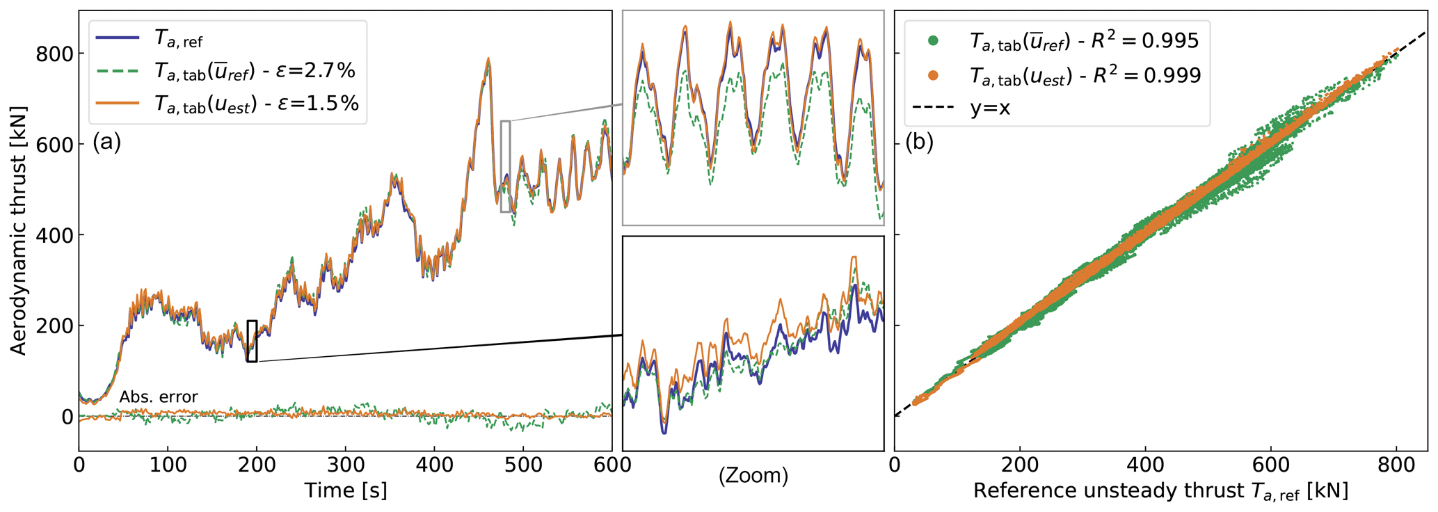
Figure 4 Comparison of aerodynamic thrusts: T_a,ref, obtained from a reference simulation; $T_{\mathrm{a},\mathrm{tab}}\left({\overline{u}}_{\mathrm{ref}}\right)$, obtained from tabulated C_T and the rotor-averaged wind speed from the simulation; $T_{\mathrm{a},\mathrm{est}}=T_{\mathrm{a},\mathrm{tab}}\left(u_{\mathrm{est}}\right)$, obtained from the estimated wind speed. (a) Time series of thrust and absolute errors compared to the T_a,ref. (b) Scatterplot of the tabulated thrust compared to the reference thrust.

We observe that the thrust signal is obtained with a mean relative error of 1.5 % over the range of operating conditions considered. The use of the estimated wind speed produces thrust values closer to the reference thrust than if ${\stackrel{\mathrm{‾}}{u}}_{\mathrm{ref}}$ is used. In line with the discussions of Sect. 3.1, this supports the fact that the estimated wind speed provides an effective velocity that is consistent with the instantaneous state of the rotor but different from the rotor-averaged wind speed. However, it is also possible that compensating errors are at play, or that the thrust is less sensitive to changes in wind speed or drivetrain dynamics than the torque. Despite these open questions, we continue by assuming that the method provides thrust estimates with sufficient accuracy.

3.3 Reduced model of the mechanical system

In this section, we compare the 2-DOF mechanical model presented in Sect. 2.1 to the advanced OpenFAST model consisting of 16 DOFs. As mentioned in Sect. 2.1, we first improve the generalized force formulation acting on q_t. We adopt the notations from Fig. 2. The resulting force and moment at the tower top are written as ℱ_N and ℳ_N. The contribution of this load to the generalized force is ${\mathit{f}}_N={\mathbf{B}}_N\cdot [{\mathbf{F}}_N$; ℳ_N], where, according to the virtual work principle, B_N is the velocity transformation matrix that provides the velocity of point N as a function of other DOFs. Further details on this formalism are provided in Branlard (2019a). For the single-tower DOFs considered, the B matrix consists of the end values of the shape function deflection and slope (i.e., ${\mathbf{B}}_N=\left[{\mathrm{\Phi }}_{\mathrm{t},\mathrm{1}}\right(L_{\mathrm{t}})$, 0, 0, 0, ν₁, 0], where L_t is the length of the tower, and ν₁ is $\frac{\mathrm{d}{\mathrm{\Phi }}_{\mathrm{t},\mathrm{1}}}{\mathrm{d}z}\left(L_{\mathrm{t}}\right)$). The shape functions are normalized at their extremity (i.e., ${\mathrm{\Phi }}_{\mathrm{t},i}\left(L_{\mathrm{t}}\right)=\mathrm{1}$) so that the generalized force is

$$\begin{array}{}\text{(21)}& f_N={\mathcal{F}}_{x,N}+{\mathit{\nu }}_{\mathrm{1}}{\mathcal{M}}_{y,N}.\end{array}$$

We assumed that the main forces acting at the tower top are the aerodynamic thrust and the gravitational force from the rotor nacelle assembly (RNA) mass, M_RNA. We then obtain the loads as

$$\begin{array}{}\text{(22)}& \begin{array}{rl}{\mathcal{F}}_{x,N}& =T_{\mathrm{a}}\cos \left({\mathit{\alpha }}_y+{\mathit{\theta }}_{\mathrm{tilt}}\right),{\mathcal{M}}_{y,N}=T_{\mathrm{a}}\left[x_{NR}\sin {\mathit{\theta }}_{\mathrm{tilt}}\right.\\ & \left.+z_{NR}\cos {\mathit{\theta }}_{\mathrm{tilt}}\right]+g{M}_{\mathrm{RNA}}\left[x_{NG}\cos {\mathit{\alpha }}_y+z_{NG}\sin {\mathit{\alpha }}_y\right],\end{array}\end{array}$$

where, using Fig. 2, θ_tilt is the tilt angle of the nacelle; NR is the vector from the tower top to the rotor center, where the thrust is assumed to act; NG is the vector from the tower top to the RNA center of mass; g is the acceleration of gravity; and α_y is the y rotation of the tower top induced by the tower bending. For a single-tower mode, α_y(t) equals q_t(t)ν₁. The linearization of Eqs. (21) and (22) for small values of q_t leads to

$$\begin{array}{}\text{(23)}& \begin{array}{rl}{f}_N& =q_{\mathrm{t}}\left\{-T_{\mathrm{a}}{\mathit{\nu }}_{\mathrm{1}}\sin {\mathit{\theta }}_{\mathrm{tilt}}+{\mathit{\nu }}_{\mathrm{1}}^{\mathrm{2}}g{M}_{\mathrm{RNA}}{z}_{NG}\right\}+\left(T_{\mathrm{a}}\cos {\mathit{\theta }}_{\mathrm{tilt}}\right)\\ & +T_{\mathrm{a}}{\mathit{\nu }}_{\mathrm{1}}\left[x_{NR}\sin {\mathit{\theta }}_{\mathrm{tilt}}+z_{NR}\cos {\mathit{\theta }}_{\mathrm{tilt}}\right]+{\mathit{\nu }}_{\mathrm{1}}g{M}_{\mathrm{RNA}}{x}_{NG},\end{array}\end{array}$$

where the term in parentheses is the main contribution, which justifies the use of T_a in Eq. (1); the term in curly brackets acts as a stiffness term. The presence of T_a in this term introduces an undesired coupling, and this term is kept on the right-hand side of Eq. (1). It is noted that the vertical force, ℱ_z,N, contributes to the softening of the tower. The main softening effect attributed to the RNA mass is included in the stiffness matrix, as described in Branlard (2019a). The contribution of the thrust to the softening, as well as an additional contribution of quadratic velocity forces to the generalized force, is neglected.

We obtain the other elements of the 2D model from the OpenFAST input files. We use the YAMS library (Branlard, 2019a) – which can take as input an OpenFAST model and thus use the same shape functions – to obtain the mass, stiffness, and damping matrix of Eq. (1). We use velocity transformation matrices to convert individual component matrices (e.g., blades, nacelle) into the global system matrices. The mass matrix thereby comprises the inertia terms from the tower and RNA. We tuned the damping of the 2-DOF model using simple “decay” simulations to include the aerodynamic damping contribution. The simulation used for validation consists of a linear ramp of wind speed from 0 to 10 m s⁻¹ in the first 100 s and a sudden drop to 6 m s⁻¹ at 200 s. The aerodynamic loads and the generator torque are extracted from the OpenFAST simulation and applied as external forces to the reduced-order model. Time series of tower-top positions, rotational speed, and tower-bottom moments are compared in Fig. 5.

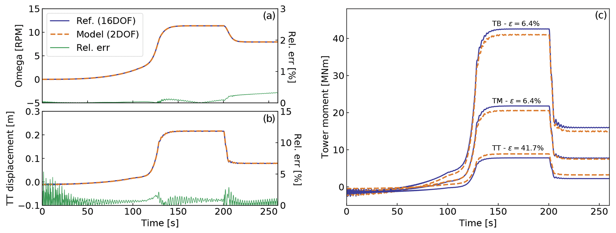
Figure 5 Simulation results using OpenFAST (16 DOFs) and the reduced 2-DOF model. (a, b) Rotational speed and tower-top (TT) displacements. (c) Tower moments at three different heights: tower bottom (TB), tower middle (TM), and tower top (TT). The tower-bottom moment is taken at 5 % height above the ground and not exactly at the ground.

We observe that the rotational speed is well captured, indicating that the rotational inertia is properly set but also indicating that the drivetrain torsion does not have a strong impact for this simulation. The overall trend of the tower-top displacements is also well captured, though more differences are present as a result of missing contributions from additional blade and tower DOFs, missing nonlinearities, and quadratic velocity forces.

We use the method from Sect. 2.5 to estimate the bending moments along the tower from the tower-top displacement. The results shown on the right of Fig. 5 indicate that the overall trends and load levels are well estimated, but some offsets are observed, which are a function of height. A contribution to the moment may be missing in the current model. This is taken into consideration when analyzing the results from the Kalman filter analysis.

4 Application to wind turbine tower load estimation

Some of the individual models presented in Sect. 2 were briefly validated in Sect. 3. In this section, we use the augmented Kalman filter described in Sect. 2.3, combining the different models together with the measurements. We implement the state and output equations given in Eqs. (2) and (3). We discretize the state equation according to Eq. (14). Results from the Kalman filter simulation, which combines a set of measurements with a model, is referred to as “KF estimation”. The values used for the covariance matrices, Q and R, are discussed in Sect. 5.

4.1 Ideal cases without noise

The same simulation as the one presented in Sect. 3.1 is used, which extends from Region 0 to Region 3. The measurements sampled at 20 Hz are taken directly from the OpenFAST simulation and not from a field experiment. This is obviously an ideal situation because no noise or bias are present in the measurements. Further, the OpenFAST and Kalman filter models are based on the same parameters, such as the mass and stiffness distribution. In Fig. 6, we compare the states and tower loads estimated using the Kalman filter model with the simulation results.

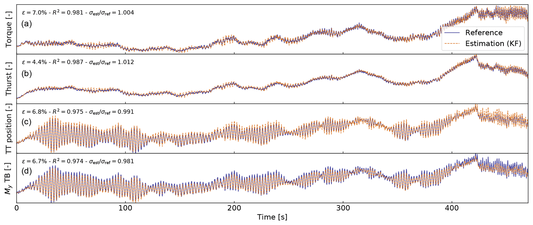
Figure 6 Comparison of signals simulated by OpenFAST (reference) compared with the ones estimated with the Kalman filter model. From (a) to (d): dimensionless time series of aerodynamic torque, aerodynamic thrust, tower-top displacement, and fore–aft tower-bottom moment.

The signals are observed to be well estimated by the Kalman filter model over the entire range of operating regions. The error observed for the tower-bottom moment is in the range of errors observed for the isolated mechanical system (Sect. 3.3).

We ran a turbulent simulation at an average wind speed of 14 m s⁻¹ with a turbulence intensity of 0.14 to illustrate the differences in the power spectral density of the signals. The results are displayed in Fig. 7 and commented on further.

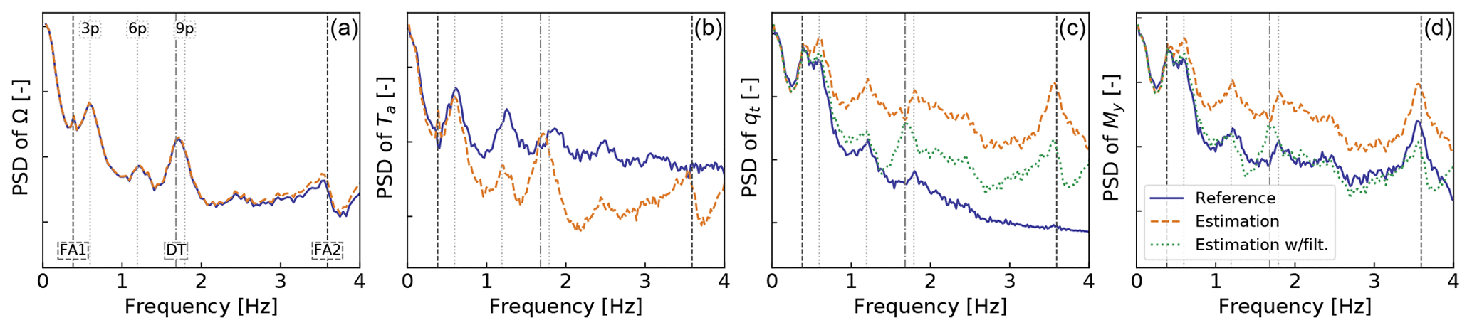
Figure 7 Power spectral density (PSD) of signals simulated by OpenFAST and estimated with the Kalman filter model for a turbulent simulation at 14 m s⁻¹. From (a) to (d): rotational speed, thrust, tower-top displacement, and tower-bottom fore–aft moment. Ticks on the y axis represent 2 decades. The main system frequencies are marked with vertical lines: FA modes, DT, and multiples of the rotational frequency p=0.2.

Frequencies that are not in the mechanical system (e.g., the second fore–aft, FA, mode and the drivetrain torsion, DT) are still “captured” by the estimator via the measurements. The rotational speed is directly observable by the Kalman filter, so the signal is obviously well estimated. The thrust is estimated based on the rotational speed and thus exhibits similar frequencies as the rotational speed, which is not the case for the reference thrust signal. The integration of the acceleration into the tower-top position (q_t) shows a higher frequency content than the reference signal. The second FA frequency has a strong energy content in the estimated q_t signal. This frequency content comes from the acceleration signal, but it is not sufficiently captured and damped by the model, which does not represent the second mode. A moving average filter of a period of 1 s was introduced to reduce the high-frequency content of the acceleration. The results are labeled “Estimation w/filt.” on the figure. The analysis of the moment spectrum given on the right of Fig. 7 indicates that the frequencies are well captured, but the overall content at frequencies beyond the first FA mode is too high. This is indicated by the values of the equivalent loads, which are 20 and 30 MNm for the reference and estimated signal, respectively, using a Wöhler slope of m=5. The low-pass filter on the acceleration signal greatly improves the spectrum of M_y. The error in equivalent loads is further quantified in Sect. 4.2.

4.2 Simulations with noise

The simulations presented in Sect. 4.1 used the simulated values from OpenFAST as measurements. In this section, a Gaussian noise is added to each of the OpenFAST signals to account for measurement uncertainties. The noise level is taken as 10 % of the standard deviation of the signal simulated by OpenFAST. A noise level of 20 % is referred to as “large noise”. We performed OpenFAST simulations for 10 wind speeds, with six different turbulent seeds for each wind speed. We applied a noise level to these simulation results prior to feeding them to the Kalman filter estimator. Cases with or without applying the low-pass filter to the (noisy) acceleration input were tried. Figure 8 displays results for the error in equivalent load and standard deviation of the tower-bottom moment. The equivalent loads are estimated using a Wöhler slope of m=5.

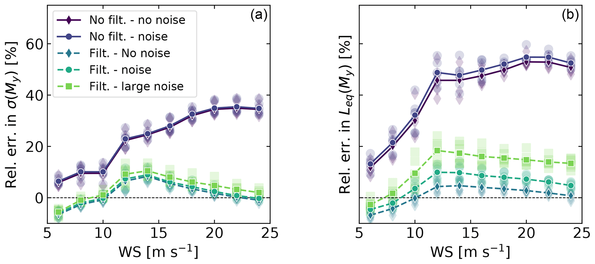
Figure 8 Comparison of the equivalent load and standard deviation of the tower-bottom moment as obtained by OpenFAST or as estimated from the Kalman filter estimator, for different noise levels and with or without a filter on the acceleration input. (a) Error in standard deviation. (b) Error in equivalent load. A positive value indicates that the estimator is overestimating. Individual markers indicate a simulation at a given wind speed and turbulence seed number. Lines indicate the mean values.

As expected, the errors in standard deviation and equivalent loads follow similar trends. Errors without filtering are severalfold larger than when the acceleration is filtered. Without noise, the equivalent loads are estimated with ±8 % error. The error increases with the noise level, and the equivalent loads appear to be mostly overestimated. Further tuning of the filter and the covariance matrices involved in the Kalman filter may reduce the error. Further discussions are provided in Sect. 5.

4.3 Computational time

We wrote this framework in the noncompiled Python language and ran the code on a single CPU. The average computational time for a 10 min period of measurements at 20 Hz was 37 s. Doubling the frequencies and the number of DOFs would still keep the computational time severalfold smaller than real time. The expensive part of the algorithm is the nonlinear solve needed to find the optimal wind speed (Eq. 16).

5 Discussion and future work

5.1 General limitations

The main limitation of the method lies in its dependency on the measurements and the numerical wind turbine model. Despite the Kalman filter being an optimal estimator that continuously adapts to its inputs, significant errors in the measurements or model would lead to unusable results. Complex online systems would be required to alleviate this issue, for instance, by continuously assessing the measurement quality, updating the wind turbine model parameters, and adapting the estimator model. More specific limitations are discussed in the subsequent paragraphs.

5.2 Digital-twin concept

A complete digital replica of a continuous system would require an infinite number of variables to represent it, which cannot be achieved. The level of detail and complexity of a digital twin is thereby chosen based on its potential application. This article was limited to the estimation of the wind speed, the integrated aerodynamic loads, and few structural degrees of freedom. This partial set provides relevant inputs for structural-dynamics applications, such as the estimation of the tower fatigue. Other applications would add more modules to the digital twin.

5.3 Digital-twin implementation

The model presented in this article was implemented such that it could be used as an online digital twin. Nevertheless, it was not connected to a real wind turbine. Such implementation would require a server running continuously and having access to the data stream from a real turbine. Additional implementation steps would be necessary to handle possible communication disruptions, server maintenance, and data storage.

5.4 Measurements

The results presented in the current study remained within the simulation realm. The accuracy of the method under uncertain conditions was partly quantified using various noise levels. Future work will evaluate the model using field measurement data.

5.5 Model choices

A Kalman filter technique was chosen for this study, but other load estimation techniques may be used, such as lookup tables, modal expansion, machine learning, neural networks, polynomial chaos expansion, deconvolution, or load extrapolation. For the Kalman filter model, a certain level of choice is present as to whether the loads are placed as an input or within the state vector, as mentioned in Sect. 2.3. A consequence is that different load models may also be implemented, such as models of higher order than the one used in Eq. (8). In the current study, a “random walk” force model was used for the torque, and the thrust was set as a dependent variable of the torque. However, these loads are functions of the axial inductions, which are typically assumed to follow a second-order model referred to as “dynamic wake”. A linearization of this model could be applied to the aerodynamic thrust and torque and potentially improve the performance prediction of the Kalman filter.

5.6 Nonlinearities and time invariance

This study assumed a linear form of the equation of motion and that the system matrices were time-invariant. Despite this crude assumption, reasonable results were obtained. Further improvements are likely to be obtained if these assumptions are lifted. A simple approach would consist of updating the system matrices at some given interval based on a slow moving average of the wind speed or the tower-top position. An advanced method would use filtering methods that are adapted to nonlinear systems, such as extended Kalman filters or particle filters. This approach would, however, greatly increase the computational time. A shortcoming of the current approach is that the linear form of the equation was established “by hand”. A systematic approach will be considered in the future using the linearized form of the state matrices returned by OpenFAST, which would include aerodynamic damping directly.

5.7 Degrees of freedom and offshore application

The general formalism presented in Sect. 2 can be applied to more degrees of freedom than the 2-DOF model used by adding more shape function for the tower and including side–side motion, yaw, tilt, shaft torsion, and blade motions. Improvements on the method are expected to be achieved by increasing the number of measurements and states. The results from the 2-DOF model appeared encouraging enough to limit ourselves to this set, but future work will consider the inclusion of additional DOFs. In particular, transverse acceleration measurements and states could help capture the rotor asymmetric loading. The extension of the method to offshore application could be done by adding extra degrees of freedom for the substructure or by using shape functions that represent the entire support structure. The generalized force induced by the wave loading would need to be included. This force may be modeled based on the wind speed or assumed to be part of the model noise (see Sect. 2.3).

5.8 Model tuning

Apart from the choices of degrees of freedom and model formulation, there remains a part of model tuning through the choice of covariance matrices and the potential filtering done on the measurements. As shown in Sect. 4.2, the filtering of the acceleration was observed to greatly improve the performance of the model. A time constant of 1 s was chosen empirically for the filter, but this value may need to be adapted for other applications. The choice of values used for the covariance matrices is usually the main source of criticism for Kalman-filter-based models. Indeed, these values have a strong influence on the results, and they are usually tuned empirically. For the current method to be successfully applied to various wind plants, an automatic tuning procedure is required. In the current study, the covariance matrices of the process were set automatically based on the value of the standard deviation of the simulated signal at rated conditions. For the measurements, these values were divided by 2. We found that this procedure led to satisfactory results. A sensitivity study should be considered in future work to give further insight on the procedure, particularly if more states and measurements are used.

5.9 Wind speed estimation and standstill and idling condition

The wind speed estimation model presented in Sect. 2.4 is limited to cases where the turbine is operating. Also, the accuracy of this model is crucial for the determination of the thrust, which in turn determines the tower-top position and the tower loads. The nacelle velocity was omitted in the current study and could be considered in future studies. The industry has great expertise in wind speed estimation, and improvements on the algorithm would benefit the model presented in this article.

5.10 Airfoil performance

The performance of the airfoils is a large source of uncertainty that was not addressed. The thrust was determined using tabulated C_T data, which may be significantly affected by the airfoil performance, which in turn is affected by blade erosion or other roughness sources and additional uncertainty in the aerodynamic modeling. Further improvement of the model is thus required to provide an accurate determination of the thrust that would account for such unknowns. Air density should also be considered for a correct account of the loading if a tabulated approach is used.

6 Conclusions

In this article, we presented a general approach using Kalman filtering to estimate loads on a wind turbine, combining a mechanical model and a set of readily available measurements. The main source of inaccuracy of the method is related to the inaccuracy of the measurements and the mechanical model. We established an open-source framework in the hope that it will be further applied for real-time fatigue estimation of wind turbine loads, providing inspiration for a digital-twin concept. As an example, we presented the equations for a 2-DOF system of a wind turbine, and this system was used throughout the article. The study focused on the estimation of tower bending moment and in particular the associated damage-equivalent load. Based on simulation results, we observed that the estimator was able to capture the damage-equivalent loads with an accuracy on the order of 10 %. Future work will address the following points: use of field measurements, offshore application of the method, increased number of DOFs, automatic covariance tuning, improved wind speed estimation in standstill, improved thrust determination in off-design conditions, and use of a linearized model obtained from an aeroservoelastic tool.