the Creative Commons Attribution 4.0 License.
the Creative Commons Attribution 4.0 License.
 | 05 Nov 2020
Laminar-turbulent transition characteristics of a 3-D wind turbine rotor blade based on experiments and computations
Helge Aagaard Madsen
Niels Nørmark Sørensen
Jens Nørkær Sørensen
Laminar-turbulent transition behavior of a wind turbine blade section is investigated in this study by means of field experiments and 3-D computational fluid dynamics (CFD) rotor simulations. The power spectral density (PSD) integrals of the pressure fluctuations obtained from the high-frequency microphones mounted on a blade section are analyzed to detect laminar-turbulent transition locations from the experiments. The atmospheric boundary layer (ABL) velocities and the turbulence intensities (T.I.) measured from the field experiments are used to create several inflow scenarios for the CFD simulations. Results from the natural and the bypass transition models of the in-house CFD EllipSys code are compared with the experiments. It is seen that the bypass transition model results fit well with experiments at the azimuthal positions where the turbine is under wake and high turbulence, while the results from other cases show agreement with the natural transition model. Furthermore, the influence of inflow turbulence, wake of an upstream turbine, and angle of attack (AOA) on the transition behavior is investigated through the field experiments. On the pressure side of the blade section, at high AOA values and wake conditions, variation in the transition location covers up to 44 % of the chord during one revolution, while for the no-wake cases and lower AOA values, variation occurs along a region that covers only 5 % of the chord. The effect of the inflow turbulence on the effective angle of attack as well as its direct effect on transition is observed. Transition locations for the wind tunnel conditions and field experiments are compared together with 2-D and 3-D CFD simulations. In contrast to the suction side, significant difference in the transition locations is observed between wind tunnel and field experiments on the pressure side for the same airfoil geometry. It is seen that the natural and bypass transition models of EllipSys3D can be used for transition prediction of a wind turbine blade section for high-Reynolds-number flows by applying various inflow scenarios separately to cover the whole range of atmospheric occurrences.
- Article
(5533 KB) - Full-text XML
- BibTeX
- EndNote


As the wind turbine technology develops and the size of modern wind turbines grows steadily, the design process becomes highly dependent on the availability of accurate aerodynamic prediction tools. The power output and the loads on the blade are affected by the aerodynamic characteristics such as lift-to-drag ratio. It is known that the skin friction drag of a turbulent boundary layer is much higher than the one of a laminar boundary layer, which makes it critical to identify which part of the flow acting on the surface is laminar, transitional, or turbulent.
The most common approach in current aerodynamic prediction tools is to use fully turbulent models for the entire boundary layer on blades/airfoils, ignoring the transitional process (Sørensen, 2009). This causes an incorrect prediction of the lift and drag forces and the stall angles. Moreover, it is seen that the transition on a wind turbine airfoil occurs over a substantial part, varying between 0 % and 30 %, of the chord (Özçakmak et al., 2019). Therefore, accurate prediction of the laminar-turbulent transition process is critical for design and prediction tools to be used in the industrial design process, particularly for the high Reynolds numbers experienced by modern wind turbines.
For many years, a large number of experimental, numerical, and theoretical studies have been devoted to laminar-turbulent transition, with the low drag laminar region being separated from the turbulent region where drag increases dramatically (Arnal et al., 1998). The transition process starts with receptivity of the disturbances like Tollmien–Schlichting (T–S) waves triggered in the laminar boundary layer, followed by linear and nonlinear instabilities ending up with turbulent spots, leading eventually to turbulent flow. In linear stability theory, it is assumed that the free-stream turbulence and other disturbances are small. On the other hand, it is seen that in the existence of large external disturbances, linear disturbance growth can be bypassed; this type of transition is defined as “bypass transition” (Morkovin, 1985). Through years, both empirical correlations (Michel, 1951; Eppler, 1978) and semiempirical methods are developed by Dini et al. (1992) for the prediction of the boundary layer transition. Semiempirical transition detection of incompressible 2-D boundary layers by the eN method based on linear stability theory was introduced by Van Ingen (1956) and independently by Smith and Gamberoni (1956). Since then, different versions were developed and databases are generated for more complex problems. For instance, a database method is developed based on the stability diagrams calculated by Arnal for Hartree–Stewartson solutions of the Falkner–Skan equation. Wazzan et al. (1968) and Kümmerer (1973) published improved stability calculations for attached Falkner–Skan velocity profiles. Envelope methods (Gleyzes et al., 1983; Drela and Giles, 1987) and approximate methods (Stock and Degenhart, 1989) were developed. The effect of disturbance environment on the transition process has been studied by Morkovin (1969) and Reshotko (1969).
The transition prediction models implemented in Navier–Stokes solvers can be categorized into algebraic–integral models and transport models (Davis et al., 2005). The first category includes empirical models, approaches based on stability theory using Orr–Sommerfeld equations, and simplified eN stability models. These models requires boundary layer information that can be obtained by integration of the boundary layer quantities or using velocity profile databases to solve integral boundary layer equations. The second category includes transition models based on the solution of the transport equations, such as the γ−Reθ (Langtry, 2006; Menter et al., 2006) model and three-equation model (Walters and Leylek, 2004). Transition can be predicted within direct numerical simulation (DNS) or large-eddy simulations (LES) despite the fact that cost of the simulations increases rapidly with Reynolds number (Diakakis et al., 2019). PSEs (parabolized stability equations) that can include nonparallel and nonlinear effects are also used for the stability analysis, having less resource requirements compared to DNS (Bertolotti et al., 1992; Herbert, 1997). There are also hybrid approaches such as DES (detached-eddy simulation) that are used with transition models. The transition phenomenon itself is a highly nonlinear problem, but with a semiempirical extension, the eN method is commonly used since it can predict the trends in variation in transition position accurately. For the industrial applications, the eN method together with empirical criteria for transition mechanisms that are not covered by this approach, such as bypass and attachment line transition, keeps its place as a practical method (Krumbein, 2009). The design process for the wings and airfoils still requires the use of laminar-turbulent transition modeling in Reynolds-averaged Navier–Stokes (RANS) solvers. The current analysis involves a coupling of the eN transition model with the RANS solver considering its accuracy for high-Reynolds-number flows in wind turbine applications (Sørensen et al., 2014).
The experimental studies on laminar-turbulent transition on aerospace applications goes back a long way compared to the research conducted on wind turbines. While the inflow turbulence intensity for an airplane wing in cruise is lower than the one experienced in a wind tunnel, it is higher for rotating machinery or wind turbine rotors (Hernandez et al., 2012). Transition analysis performed for wind tunnel experiments in controlled conditions includes measurements on wind turbine airfoils equipped with pressure taps and sensors, a balance system, and a wake rake (Yilmaz et al., 2017); infrared thermography (Joseph et al., 2016); rotating turbine blade equipped with pressure sensors, strain gauges, a balance system, and particle image velocimetry (Schepers and Snel, 2007); rotating wind turbine; and wind turbine blade experiments by oil visualization, stethoscope, and flush-mounted unsteady pressure sensors (Lobo et al., 2018); and wind turbine airfoil with pressure sensors and high-frequency microphones (Özçakmak et al., 2019).
In addition to the DAN-AERO experimental campaign (Madsen et al., 2010; Troldborg et al., 2013), on which the current analysis is based, there have been other field experiments on boundary layer transition on rotating wind turbine blades using microphones glued on the surface (Jan Leendert Van Ingen and J. Gerard Schepers, personal communication, 2020), hot film, pressure tubes (Schwab et al., 2014; Schaffarczyk et al., 2017), microphones on the suction side, and the ground-based thermographic cameras (Reichstein et al., 2019). All these experiments pointed to the fact that more field experiments are needed on the wind turbine blades in order to characterize the transition behavior with inflow turbulence and rotational effects. Moreover, determining the relevant frequency ranges for the atmospheric turbulence and the occurrence of the T–S waves under real atmospheric conditions is needed in order to investigate the combined effects of the turbulent wind and the blade rotation on transition. Modern wind turbines usually operate in wind farms where the inflow is affected by the wake of the upstream turbines. They are also exposed to high free-stream atmospheric turbulence and wind shear. The differences in the transition behavior of an airfoil section tested in a controlled 2-D wind tunnel environment and a blade tested in 3-D field experiments at real operational conditions are discussed in previous works and it is seen that a full rotor blade section exhibits different transition characteristics than in the 2-D case (Madsen et al., 2019a; Schaffarczyk et al., 2018). The difference between the design conditions for rotor and airfoils and the real operating conditions leads to inaccurate predictions of the loads and the performance as observed in previous studies from Sørensen (2009) and Chaviaropoulos et al. (2015).
In this study, the transition characteristics of the LM 38.8 blade on the NM80 2.3MW wind turbine are analyzed by field experiments (DAN-AERO project) and computations with the DTU in-house CFD EllipSys code (Sørensen, 1995; Michelsen, 1992, 1994). The present experimental analysis is based on high-frequency microphone measurements that enable the acquisition of data at higher sampling frequencies and allows a higher resolution (with the number of microphones placed on both upper and lower surfaces) than the previous studies. This paper is focused on the analysis of the DAN-AERO 3-D transition rotor measurements in a wind farm and the validation of the transition models in the EllipSys3D CFD in-house solver using these experimental data. The atmospheric turbulence, wind shear, and wake effects on transition behavior of a wind turbine blade section are discussed. The effect of these parameters on the effective angle of attack and velocity on the blade section as well as their potential direct effect on transition is discussed. Comparison of the field experiments with the CFD simulations enlightens the transition behavior of the wind turbine blades and enables improvement of the design and aerodynamic prediction tools.
The main objective of the DAN-AERO project was to establish an experimental database for aerodynamic, aeroelastic, and aeroacoustic issues that are significant for the design and operation of megawatt-size wind turbines (Bak et al., 2010). The laminar-turbulent transition investigation of this campaign contains both 2-D wind tunnel tests (Madsen et al., 2010) as later analyzed by Özçakmak et al. (2018, 2019), and 3-D field experiments (Troldborg et al., 2013).
In this study, field experiments are analyzed in order to investigate the laminar-turbulent transition characteristics of a 3-D rotor blade. The tested turbine is placed at a wind farm in Tjæreborg, Denmark, which consists of eight turbines in two rows. The test turbine is a 2 MW NM-80 wind turbine with an LM 38.8 blade. The rotor diameter is 80 m. The site and the test turbine (denoted as “NM80”) are presented in Fig. 1. The wake cases presented in this paper are from an upstream wind turbine that is located around six rotor diameters (6 D) upstream of the test turbine.
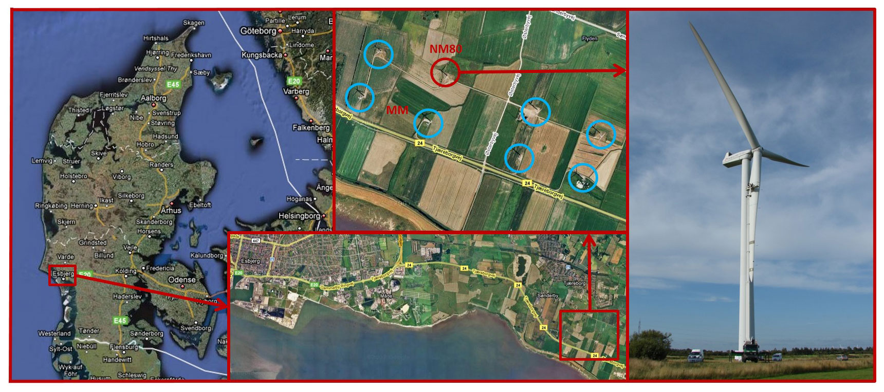
Figure 1Map of the site approx. 10 km southeast of Esbjerg (© Google Maps 2007). The test turbine, NM80, is situated in a small wind farm at Tjæreborg along with seven other wind turbines of around 2 MW in size. The other turbines are circled with blue and the test turbine is marked by the red circle. The meteorology mast is shown by the “MM” denotation in the picture.
The rotational speed, yaw, pitch, and rotor azimuth angles are measured at the nacelle. In addition to the pressure taps placed at four different sections on the blade, 56 high-frequency microphones are installed about 1 mm below the blade surface at a section 36.9 m from the hub (3.1 m from the tip of the blade). The same section is also equipped with a pitot tube for measuring the relative velocity. The pressure taps are placed 36.8 m from the hub (3.2 m from the tip) next to the microphones. The wind direction and wind speed information of the inflow is obtained from the anemometers and wind vanes placed at the meteorological mast (denoted as “MM”) 2.5 D from the test turbine; see Fig. 1. At some specific wind directions, the test turbine is in the wake of the upstream turbine, the effect of which is also discussed in this study. Both wake and no-wake conditions are analyzed.
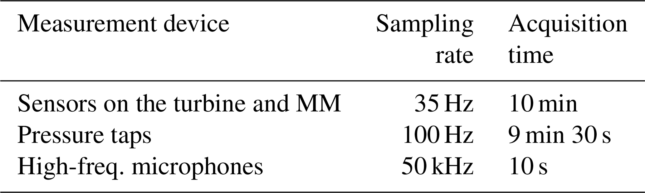
The angle-of-attack values of the field experiments presented in this article are derived from the measured normal force on the blade. The correlation between the normal force and the angle of attack is generated by the HAWC2 (Horizontal Axis Wind turbine simulation Code 2nd generation) (Larsen and Hansen, 2007) simulations which are based on the principle blade element momentum theory with an aeroelastic model of an NM80 turbine using existing polars. A previous study of Boorsma et al. (2018) has shown a good correlation between measured and computed normal forces. The acquisition properties of the instruments on the test blade and the meteorological mast are listed in Table 1.
Different 10 min series from 2 different days are used in this study with corresponding 10 s series of microphone acquisition. The turbine operated at two different pitch settings: 1.25 and 4.75∘. The pitch angle is defined as positive towards stall.
The blade section that is equipped with the high-frequency microphones features a NACA 63-418 airfoil with a chord length of 1.24 m. The turbine is operated at a constant rotational speed of 16.1 rpm (revolutions per minute) and at a fixed pitch setting. The Reynolds number is around 5 million for the tested blade section. The region of the atmospheric boundary layer where the turbines operate has varying levels of free-stream turbulence. This contributes to large external disturbances in the boundary layer of the blades. The degree of turbulence in the wind varies greatly on short timescales. Therefore, for the inflow velocities, 10 s datasets from MM measurements are used, which correspond to microphone acquisition times.
The ABL velocity profiles are averaged over 10 min (a) and over 10 s (b) corresponding to the exact time instance of the microphone dataset, presented in Fig. 2 with their standard deviations as shaded areas. In 10 s average profiles, for some of the selected cases, an increase in the velocity is observed at 57 m from the ground where the turbine hub is approximately located.
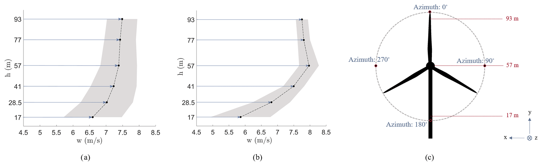
Figure 2ABL velocity profiles: (a) 10 min average; (b) 10 s average corresponding to microphone acquisition time; (c) azimuthal placement and the heights of the blade cross section at each azimuthal location.
The 2-D results shown in this paper originate from the wind tunnel experiments of the DAN-AERO project conducted in the LM wind tunnel with a reproduction of the actual blade section of the wind turbine deviating from the theoretical airfoil, the details of which are explained in a previous study of Özçakmak et al. (2019).
2.1 Data processing
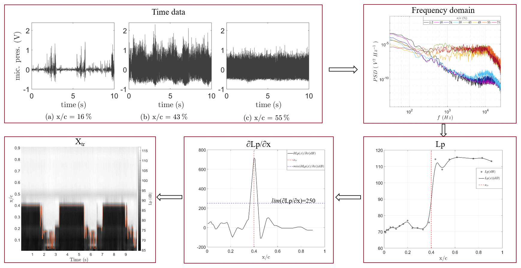
The pressure fluctuations in time domain (10 s series), obtained from high-frequency microphones placed chordwise on the blade section, are analyzed in the frequency domain by fast-Fourier-transform (FFT) analysis. The sampling frequency of the data is 50 kHz acquired over 10 s. The data are divided into smaller time segments of 0.0410 s. The window size of 4096 is used with a 50 % overlap. For each time segment, the power spectral density (PSD) is calculated by the short-time Fourier transformation analysis (Welch, 1967).
The PSD (Ps,p) of the pressure fluctuations obtained from the microphones is integrated in a frequency interval from f1=2 to f2=7 kHz (see Eq. 1). The integration within a certain frequency range gives the standard deviation (σ), which represents the total energy of the pressure fluctuations. A sudden chordwise increase in the pressure level (Lp) is considered an indication of the transition location. The reference pressure Pref is assigned to the value of 20 µPa. More details on this method and the selection procedure of the frequency interval for the integration can be found in a previous work by Özçakmak et al. (2019).
The transition location on the upper and lower surfaces is detected by the highest chordwise derivative of the pressure level as in Eq. (2). The derivatives that are above a threshold level of 250 dB are selected for transition detection.
The transition detection method is illustrated in Fig. 3. The laminar, transitional, and turbulent flows in time series and in frequency domain are illustrated at the top of the figure, and the chordwise increase in the integrated PSD and the derivative of Lp are illustrated at the bottom. The spectrogram analyses are also performed by dividing the data length (L) into k columns. The final detected transition locations can be seen from the spectrogram at the bottom left figure.
EllipSys3D is an in-house CFD solver for incompressible Navier–Stokes equations in general curvilinear coordinates by a multiblock finite-volume discretization, here applied in RANS mode. Rhie–Chow (Rhie and Chow, 1982) interpolation is used in order to avoid odd–even pressure decoupling. The third-order QUICK (Quadratic Upstream interpolation for Convective kinematics) upwind scheme is used for the convective terms. The SIMPLE (Semi-Implicit Method for Pressure-Linked Equations) algorithm is used to enforce the pressure–velocity coupling (Patankar and Spalding, 1983; Patankar, 1980). The Message Passing Interface (MPI) is used to parallelize the code for executing on distributed memory machines with nonoverlapping domain decomposition (Sørensen et al., 2011).
Mesh generation is done by the 3-D hyperbolic grid generation program HypGrid3D (Sørensen, 1998). The rotor geometry and the boundary layer of the blade surface are resolved by O–O mesh configuration. The grid consists of 256 cells in the chordwise direction, 128 cells in the spanwise direction, and 128 in the normal direction, with cell size ensuring a y+ value less than 1. The mesh has around 14 million cells. The mesh refinement study shows that the difference between the moment and forces for the finest and a coarser mesh (having one-half of the number of cells of the finest grid in all directions) is within a few percent as demonstrated in a previous study of Madsen et al. (2019b). The far-field boundary is located around 10 D away from the rotor in all directions. Due to the high tip speed ratio, in order to stabilize the simulations and enhance the convergence of the solution by small time steps, the simulations are performed by transient computations with 1200 steps per revolution. At each time step, the momentum equations are solved and a pressure correction equation is used to satisfy the continuity constraint. This process is repeated until a convergent solution is reached, and all the terms are evaluated at the next time level when the subiterations are finished.
The turbulence is modeled by the k−ω shear stress transport (SST) eddy viscosity model (Menter, 1993). The boundary layer transition prediction on the rotating wind turbine blade section is performed by the eN transition method based on linear stability theory and the bypass transition model.
In the CFD simulations, the eN transition method is applied for several flow conditions representing the field experiments. The EllipSys3D rotor simulations are performed at several free-stream velocities representing the ABL conditions at three different heights, considering both the mean and the standard deviations during the microphone acquisition time. Both the eN natural transition model with different amplification factors (N) and the bypass transition model at the corresponding atmospheric turbulence intensity values from the field experiments are simulated.
The angle of attack from the EllipSys3D simulations on the blade section is determined from the annular averaging method by determining the local induced velocities at the blade (Hansen et al., 1997; Johansen and Sørensen, 2004). In order to calculate the induced axial velocity, Vind, at the rotor plane, annular averaging of the axial velocity at several upstream and downstream locations (zi and zj) at a given radial location (in this case, the same blade section as in the microphone experiments) is performed. Then, Vind is found by the interpolation of these averaged streamwise velocities to the rotor plane. Lagrangian polynomial interpolation is used to determine the velocity at the rotor location (z=z0) as in Eq. (3).
Having calculated Vind, the effective local flow angle (α) is found from Eq. (4), where ω is the angular velocity, R is the distance to the hub from the measured tested section on the blade, and θ is the combined pitch twist angle.
The FieldView (2017) software is used in order to postprocess the EllipSys3D simulation results and to extract the annular averages of the axial velocity and for the flow visualization.
3.1 EllipSys3D semiempirical eN transition model
Transition to turbulence in EllipSys3D is governed by the semiempirical eN model (Drela and Giles, 1987), which is based on linear stability theory. The conventional eN method is a semiempirical method not considering receptivity. In the semiempirical method, while linear stability analysis is done for the governing equations; the transition is assumed to take place when N reaches a previously correlated value from the experiments. Therefore, the empirical part comes from the N value at transition, which makes the model semiempirical. In the eN method, the amplification of small disturbances is calculated for several frequencies, and the spectrum of the most amplified ones is identified. The critical N factor for each type of flow is determined empirically, and the transition point is detected from this empirical value of the critical N factor.
In the EllipSys3D code, the boundary layer parameters (the displacement thickness δ*, momentum thickness θ, and the shape factor H in Eq. 5) are needed as an input to determine the occurrence of transition. Ue is the velocity at the outer edge of the boundary layer which is determined from the Navier–Stokes computation, and y is the direction perpendicular to the wall/surface. The boundary layer thickness δ is defined as the location where u=0.99Ue. In EllipSys3D, the edge velocity (Ue) is taken as the maximum tangential velocity.
Although these boundary layer parameters can be calculated by integrating the velocity profile from the Navier–Stokes equations, it is shown by Stock and Haase (1999) that it requires an excessively fine computational grid. Therefore, the boundary layer parameters are found from the von Kármán boundary layer equations (Von Kármán, 1921).
The momentum integral equation (Eq. 6) and the combination of the kinetic energy equation with von Kármán's momentum equation (Eq. 7) are solved for H and θ. Ue is determined from the Navier–Stokes computation. In each iteration, these equations are started from the stagnation line and integrated downstream on the surface until the transition point is found.
CD is the kinetic energy dissipation coefficient () and D is the dissipation per unit area. The Un term, the velocity normal to the wall, comes from the assumption of axial symmetry. These equations are presented in terms of boundary layer parameters and the skin friction coefficient Cf, where x is the horizontal direction, τw is the wall shear stress, ρ is density, μ is the dynamic viscosity, θ* is the kinetic energy thickness, and H* is the energy thickness ratio as shown in Eq. (8).
Closures for Cf, Cd, and θ* are calculated based on Falkner–Skan velocity profiles. The stagnation line is normally found as the location where the pressure coefficient based on relative velocity is equal to 1. In order to ensure that the entire stagnation line is found at each time step, the pressure coefficient value is checked and the Navier–Stokes solution is analyzed. Along the stagnation line, Blasius flow and across the stagnation line Hiemenz flow are assumed. In this way, realistic initial values for H and θ are obtained, and the stagnation line can be located between two computational cells.
The development of the imposed wave perturbations' amplitude is computed along the boundary layer based on spatial analysis. A check is carried out during the integration of the boundary layer equations to determine whether the disturbances are amplified or damped. As neutral stability is passed, amplifications are determined for a range of temporal frequencies.
The N factor is the natural logarithm of the ratio of the disturbance amplitude at a specific location to its amplitude at the neutral stability point. Integration of the N amplitude is carried out until it reaches a certain value for which transition is said to occur. This value is set according to the turbulence degree that is present in the experimental conditions for comparison with the simulations. In order to build a relation between the turbulence level and the amplification factor, Mack's expression (Mack, 1977) is used as an estimate.
Transition to turbulence is handled by the intermittency factor (γ) when solving the Navier–Stokes equations. The eddy viscosity (μT) obtained from the turbulence model is multiplied with the intermittency factor which controls the effective viscosity (μeff=μ+γμT), where μ is the molecular viscosity.
The intermittency factor is calculated from Eq. (10). This equation is obtained by combining the statistical theory for transitional flow by Emmons (1951) and the expression that represents the production rate with Gaussian distribution using the Dirac delta function by Dhawan and Narasimha (1958) and the Chen and Thyson (1971) formulation:
where the subscript “tr” is the transition onset, ν is the kinematic viscosity, σ is here the spot propagation rate, and is the nondimensional spot formation rate, (Mayle, 1998).
The intermittency factor is calculated on the surface and then solved for the entire boundary layer and wake within the transport equation (Michelsen, 2002).
where the source term, S, is obtained by evaluating the transport terms for previously determined intermittency values.
3.1.1 Bypass transition model
When the amplitude of the disturbances are strong, such as for high free-stream turbulence or large roughness elements, the linear stages of the transition process are bypassed. In this case, transition happens in the absence of T–S waves, and the disturbances are amplified by a nonlinear process.
The approaches for modeling bypass transition in industry involves low-Reynolds-number turbulence models and models using experimental correlations that relate free-stream turbulence intensity to transition Reynolds number based on momentum thickness Reθt (Reza and Amir, 2009).
The eN method accurately predicts the transition for free-stream turbulence levels, less than 2 % for T–S-dominated transition, but for higher levels it is bypassed (Biau et al., 2007). It should be noted that transition can also be dominated by other mechanisms, for instance by a streak breakdown for turbulence levels around 0.65 % (Suder et al., 1988). The eN method in EllipSys3D can be used together with a bypass criteria. For the bypass transition model, the Suzen and Huang (2000) empirical model is used.
Abu-Ghannam and Shaw (1980) suggested that for the attached flows, transition onset can be obtained by correlating Reθ to the free-stream turbulence intensity as in Eq. (12). By maintaining the strong features of this correlation in adverse pressure gradient regions, a more sensitive response to the favorable pressure gradients is obtained by Suzen et al. (2002) by re-correlating the transition criterion to the free-stream turbulence intensity and acceleration parameter Kt.
Here, Kt is the minimum value of the acceleration parameter in the downstream direction (Michelsen, 2002), which can be expressed as , where Ut is the boundary layer velocity at onset of transition (Suzen et al., 2002). Tu is the turbulence intensity at the transition onset. Under high-turbulence-intensity conditions, this correlation fits well with adverse pressure gradient regions. In EllipSys3D, for the bypass transition cases, where turbulence intensity levels are high, this correlation is used and the criteria for natural and bypass transitions are checked simultaneously in the code. The higher of the two intermittency factors is used. Moreover, separation-induced transition is also checked with a bubble model inside the boundary layer solver.
3.2 Numerical setup
The computations are performed for three different grid levels for the 3-D simulations and five different grid levels for the 2-D case. The grid independence is ensured and the results of the finest grid are presented.
The 3-D full rotor simulations are performed as transient calculations with 1200 steps per revolution for all grid levels. The problem is approximately axisymmetric. The CFD simulation input parameters are listed in Table 2 for the finest grid level. The input k is the turbulent kinetic energy and ω is the specific dissipation for the turbulence model. Several free-stream velocities are simulated from 5.5 to 8.5 m s−1. It should be noted that, in the experiments, inflow conditions vary as a function of the blade azimuth due to the wake and wind shear. Therefore, these local inflow conditions are represented by individual CFD simulations with various wind speeds and T.I. since it is difficult to simulate spatially varying inflow conditions only by a single simulation. Moreover, at each simulation, different amplification factors (N=0.15, 3, and 7) are used in the natural transition model to represent different inflow scenarios.

The turbulence is quantified by the turbulence intensity (T.I.), which is the standard deviation of the relative velocity divided by the average relative velocity over 10 min in this case. The 10 min average of the velocity data obtained from the pitot tube on the blade is used in order to obtain the T.I. values. Various T.I. values of 2.8 %, 3.8 %, and 6.8 % are used as an input to the bypass transition model in the CFD computations. The transition point is selected to be the first location where γ⩾0.025 for both of the transition models.
4.1 Atmospheric effects on transition
The flow on the blade is affected by many parameters in the free atmosphere compared to an airfoil in a steady flow in a wind tunnel. The atmospheric flow has a substantial effect on the performance and loading of the turbines. The shear in the atmospheric boundary layer and the inflow turbulence in combination with the rotational effects create a significant deviation of the aerodynamic characteristics on the blade compared to the wind tunnel flow conditions. The effective angle of attack and velocity vary as a function of azimuth position with these parameters and cause the transition position to move constantly during rotation. These multiple effects on transition are not easy to analyze separately. For instance, the large scales of the inflow turbulence affect the effective angle of attack on the blade section but may also have a direct effect on the transition location as in the wind tunnels. Thus, analysis from the experiments in this study aims to analyze these individual effects on the transition behavior.
The spectrogram of the chordwise pressure levels on the airfoil profile tested in the wind tunnel (Fig. 4a) and wind turbine blade section (Fig. 4b) from the field experiments, featuring the same airfoil profile, are presented. The transition regions can be seen by the sudden chordwise increase in the pressure levels. Due to the low inflow turbulence in the wind tunnel ( %), no time variations in the transition position are observed for the airfoil profile. On the other hand, the transition location changes significantly for the rotor blade section through one revolution for the high-pitch case (p=4.75∘) (Fig. 4b) , deviating from the 2-D case (Fig. 4a).
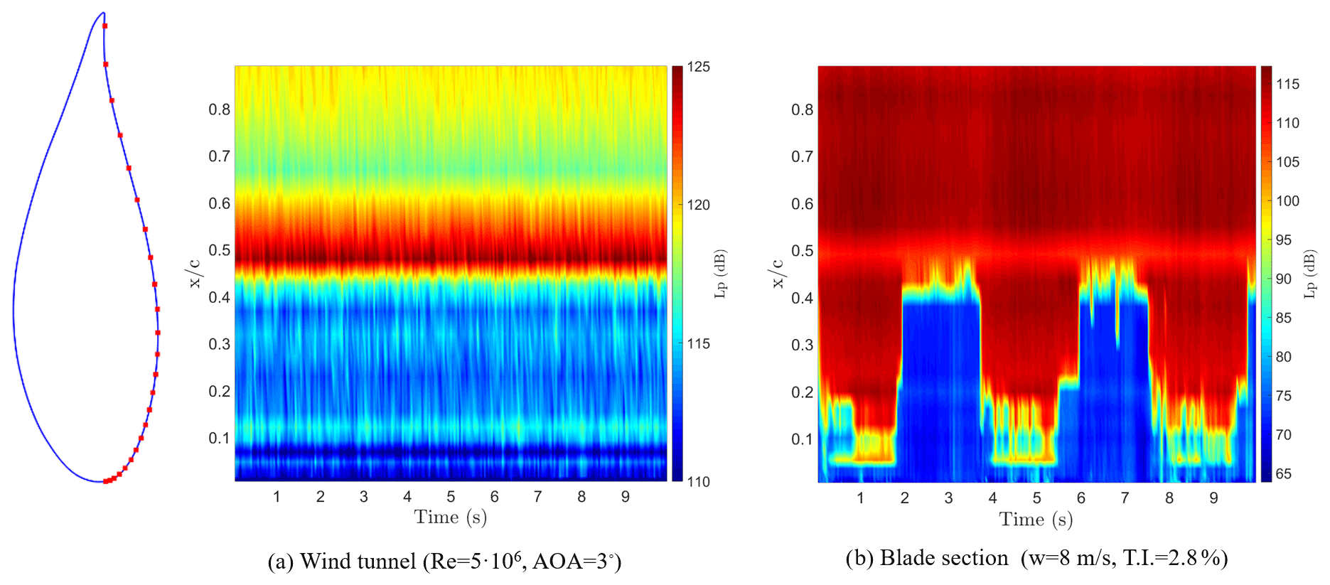
Figure 4Chordwise pressure level (Lp) spectrogram along the pressure side for airfoil tested at the wind tunnel (a) and for the blade section from the field experiments that corresponds to the Re=5.1 million and AOA varying from 3 to 8.5∘ (b). The microphone placement on the pressure side of the airfoil is shown on the left.
In order to analyze the causes of this variation, inflow characterization is performed. The PSD is integrated in the frequency range from 2 to 7 kHz for transition detection (presented in Fig. 5b). Several frequency intervals for PSD integration are also attempted in order to characterize the inflow turbulence from the microphone signals. It is seen in Fig. 5a that when the PSD is integrated in the frequency interval from 100 to 300 Hz, the microphones closer to the leading edge show high pressure levels on this frequency range, capturing the pressure response to the inflow turbulence. Therefore, this frequency range is selected for the inflow analysis. For the quantitative comparisons, a microphone located very close to the leading edge (at %) on the pressure side, in the laminar boundary layer, is selected to represent the inflow turbulence (Lp,i) that the blade section is exposed to.
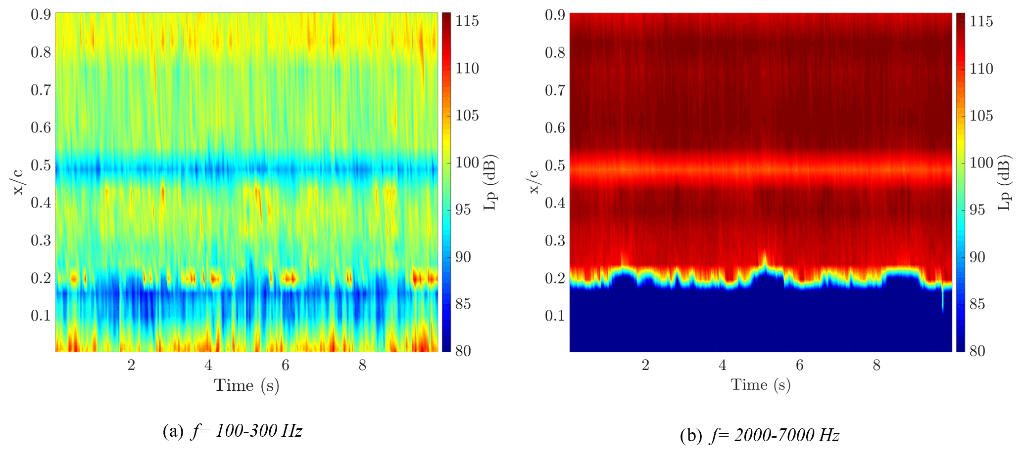
Figure 5Spectrogram of the chordwise pressure levels obtained from frequency integration limits of (a) 100–300 Hz and (b) 2–7 kHz on the pressure side, for the low-pitch case (p=1.25∘), w=6.3 m s−1, %.
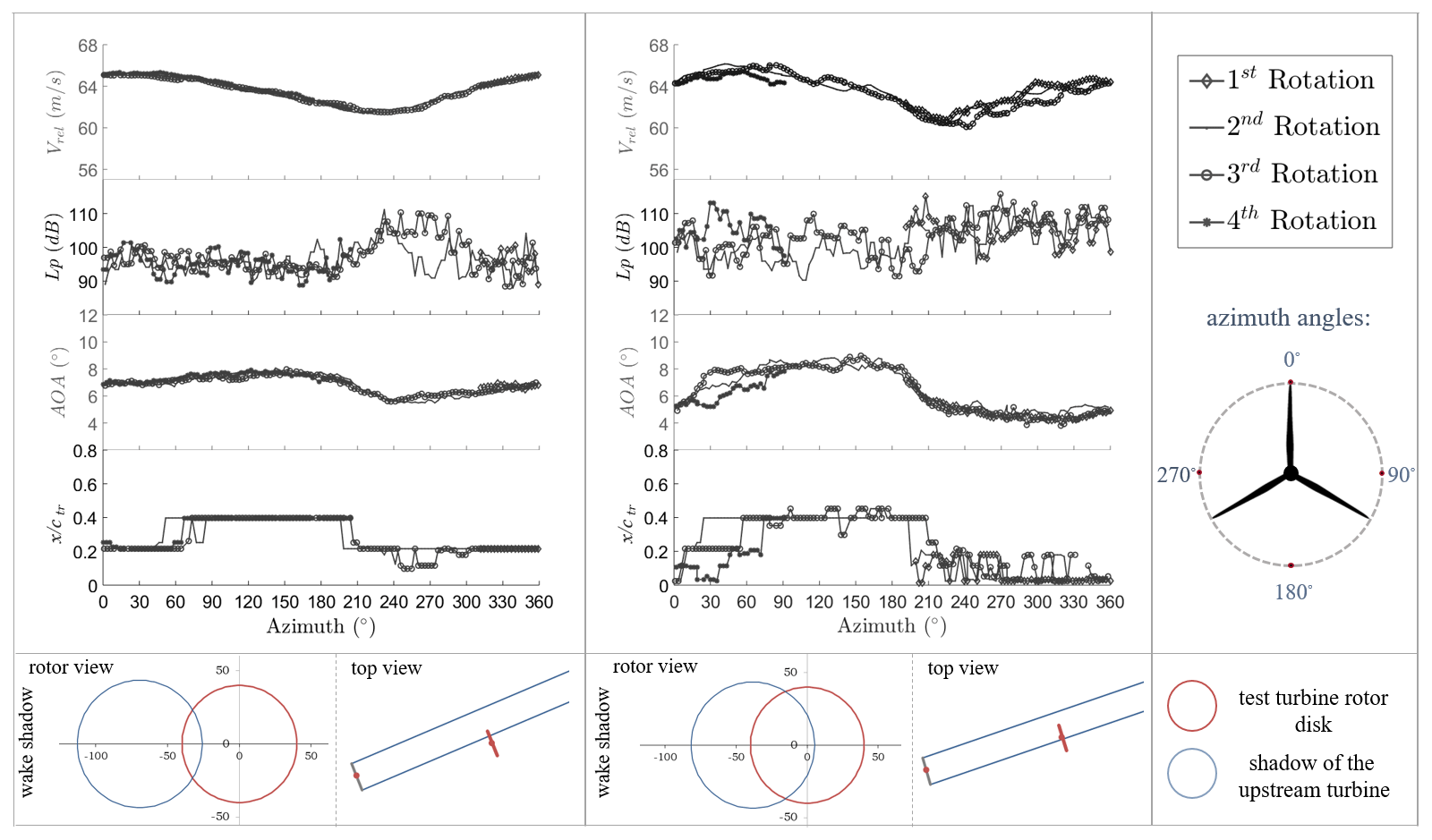
Figure 6The relative velocity (Vrel), pressure levels (Lp) of the inflow turbulence, AOA, and detected transition points (x∕ctr) for the pressure side: (left) 9 % wake shadow from an upstream turbine with U∞=7.2 m s−1; (right) 48 % wake shadow with U∞=8 m s−1; (bottom) rotor view and top view of the upstream turbine and the test turbine.
The inflow turbulence levels (Lp,i) from the microphone analysis, the relative velocity obtained from the pitot tube on the blade section, and the angle of attack, which is derived from the forces, are presented together with the detected transition points as a function of the azimuthal angle in Fig. 6. Two different cases from the measurements are shown in Fig. 6. Figure 6 on the left shows a partial-wake case (9 % wake-affected rotor area) with a free-stream velocity (U∞) of 7.2 m s−1. Figure 6 on the right demonstrates a half wake case (48 % of the rotor area covered with wake-affected inflow) with U∞=8 m s−1. Both cases have the same pitch setting and the same % obtained from the meteorological mast. The wake shadow from the rotor view and the top view is also shown at the bottom of the figure for each case. The swept area that is influenced by the wake according to the wind direction was calculated by estimating the wake expansion depending on the velocity induction factor. Each line at Vrel, AOA, Lp, and x∕ctr plots corresponding to a single revolution. For the 9 % wake case, each revolution tends to have a similar behavior; conversely, for the 48 % wake case, there are some discrepancies observed between each rotation. For both cases, it is noticeable that the decrease in relative velocity and angle of attack and the increase in the inflow turbulence lead the transition point to move closer to the leading edge at the pressure side. The tilt, yaw, and wind shear effects on AOA and Vrel are analyzed by HAWC2 simulations. Yaw misalignment (which is the difference between the angle measured on the nacelle and the wind direction measured from the meteorological mast at the same height) was checked for the cases presented in this paper. The mean absolute yaw error is found to be less than 5∘, and the effect of the maximum yaw on Vrel and AOA change is found to be no more than 1 % by HAWC2 analysis. Moreover, the wind turbine has a 5∘ tilt angle that causes 1 % change in Vrel and 0.2 % change in AOA according to this analysis. Considering that the cases presented here are not under a strong shear, and comparing those variations with the experiments, it can be concluded that the azimuthal behavior of the relative velocity and the angle of attack is governed by the inflow turbulence, mainly from the wake of an upstream turbine.
In order to distinguish the effects of the AOA and inflow turbulence, the data are divided into AOA bins. A previous study of Madsen et al. (2019a) with data from the DAN-AERO experiments shows that for several angle-of-attack bins, there is a correlation between inflow turbulence and the transition location. Increasing the turbulence content in the range of 100–300 Hz moves the transition process closer to the leading edge at the pressure side. At the suction side, transition points are detected within the first 13 % of the chord, and no correlation could be established with the inflow turbulence.
4.2 Angle-of-attack effect on transition
The relative velocity, turbulence levels (Lp,i), AOA, and detected transition points on the pressure side for two different pitch cases are compared in Fig. 7 as a function of time. These two cases belong to different measurement sets: a low-pitch case (right) with 7 m s−1 free-stream velocity with 2.6 % T.I. and a high-pitch case (left) with 7.2 m s−1 free-stream velocity with 2.8 % T.I. The high-pitch case is under 8.9 % wake from the upstream turbine while the case with low-pitch angle is under no-wake conditions. Therefore, despite some slight differences, these two cases are approximately under the same inflow conditions, which allows analysis of the effect of the angle of attack on transition. It can be seen that the transition location on the pressure side has a higher response to the rotational changes for the high-pitch case. In the low-pitch case, the transition point on the pressure side is closer to the leading edge than in the high-pitch-angle case. For the high-pitch case, the regions where the transition points move closer to the leading edge around 20 % of the chord correspond to the regions of lower angle-of-attack values, as seen in the low-pitch case.
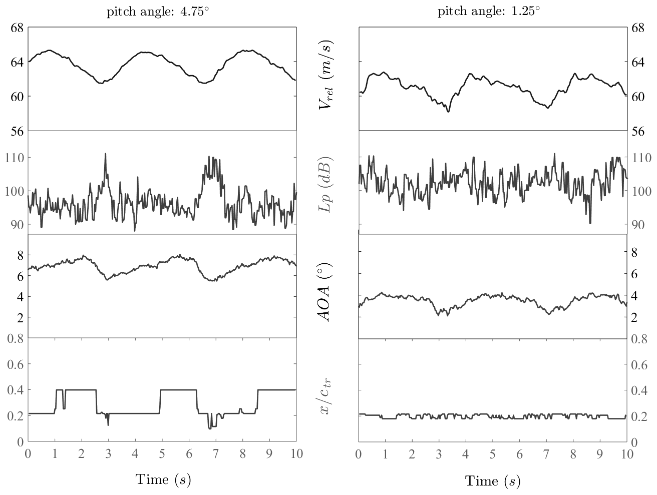
Figure 7The relative velocity (Vrel), pressure levels (Lp) of the inflow turbulence, AOA, and detected transition points (x∕ctr) for the pressure side: (left) pitch=4.75∘, 9 % wake shadow from an upstream turbine with U∞=7.2 m s−1; (right) pitch=1.25∘, no-wake case with U∞=7 m s−1.
4.3 Laminar-turbulent transition locations calculated by CFD
The vorticity structures from the rotor colored by the axial velocity (w) (top left) and the intermittency factor (γ) around the blade section, 36.8 m from the hub (top right), and on the blade for the pressure and the suction sides (bottom) are presented in Fig. 8. It can be seen from the vorticity iso-surfaces that the problem is approximately axisymmetric. From the intermittency factor visualization, the transition location on the upper and lower surfaces can be seen on the blade section (top right). The blue parts where γ equals zero show the laminar parts in the flow and the red regions (γ=1) show the turbulent parts. The γ on the suction side (bottom) of the full blade shows that the transition point moves closer to the leading edge while going from root to tip, except the innermost part of the root. For the pressure side, less change in the transition location is observed as going from root to tip on the blade compared to the suction side. The case presented here is the blade with a pitch setting of 4.75∘, a free-stream velocity of 7.2 m s−1, and an amplification factor (N) of 3.
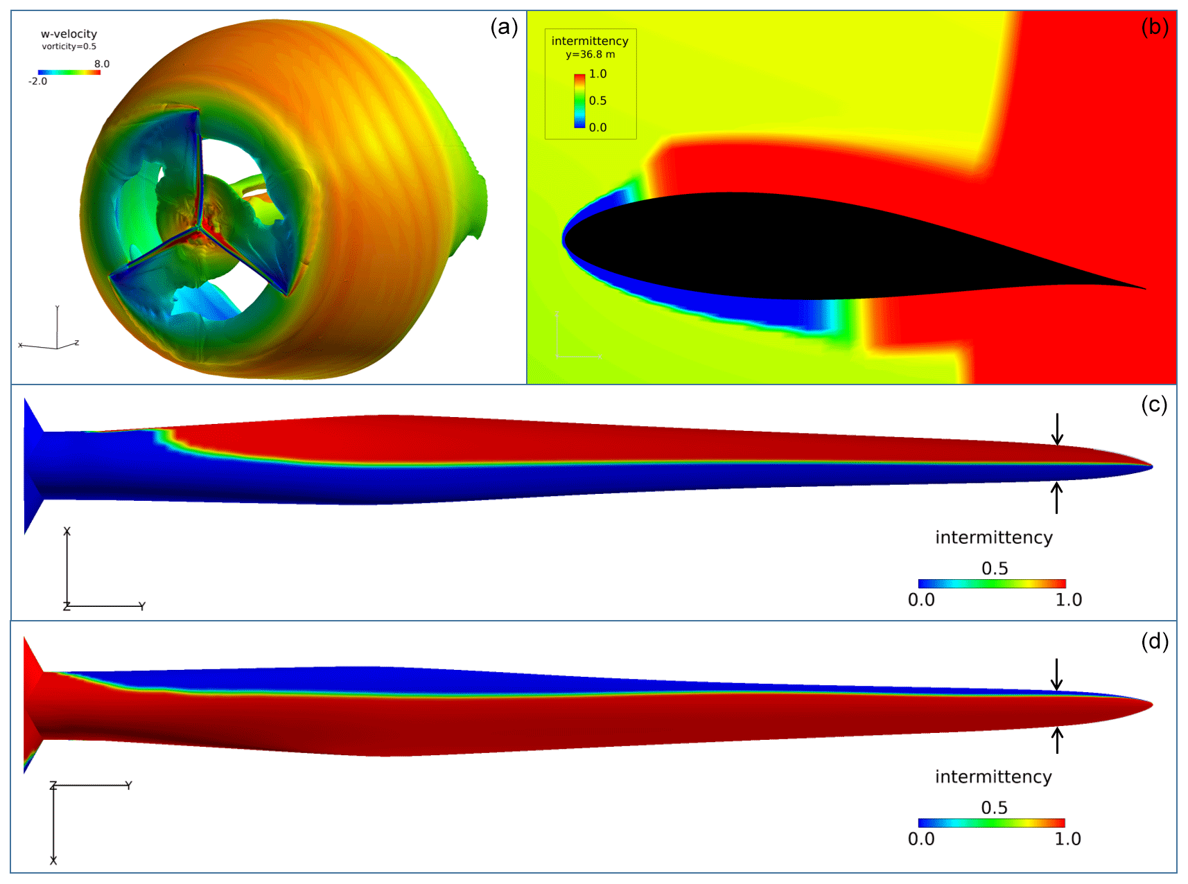
Figure 8The vorticity iso-surfaces colored by the axial velocity (a); intermittency (γ) at the blade section at y=36.8 m from the hub (b); the γ values on the pressure (c) and suction sides (d) of the blade for U∞=7.2 m s−1, N=3, p=4.75∘. (Note that the free-stream flow is in the z+ direction and the rotational speed in the −x direction for the blade at an azimuthal angle of 0∘.) (The blade section that is analyzed in the current study is highlighted by the arrows on the blade.)
4.4 Comparison between CFD and experimental results
Since the effective angle of attack in the experiments is derived from the force measurements, in order to have a direct comparison, the experimental forces are compared with the forces obtained from the EllipSys3D simulations. The Fx and Fz forces from the simulations in global coordinates are transformed to local blade section coordinates in order to obtain the chord-normal force on the blade as in the experiments. The 10 s data are extracted from the 10 min measurements that correspond to the exact microphone acquisition time to represent the cross-sectional force for the same case. This case is under 48 % wake shadow with U∞=8 m s−1. The comparison is presented in Fig. 9. Several CFD simulations obtained with various N factors and inflow velocities for natural and bypass transition models are combined to capture actual azimuthal variation behavior of the experiments. The wake shadow falls in the azimuthal range from 200 to 340∘ for this case from the measurements.
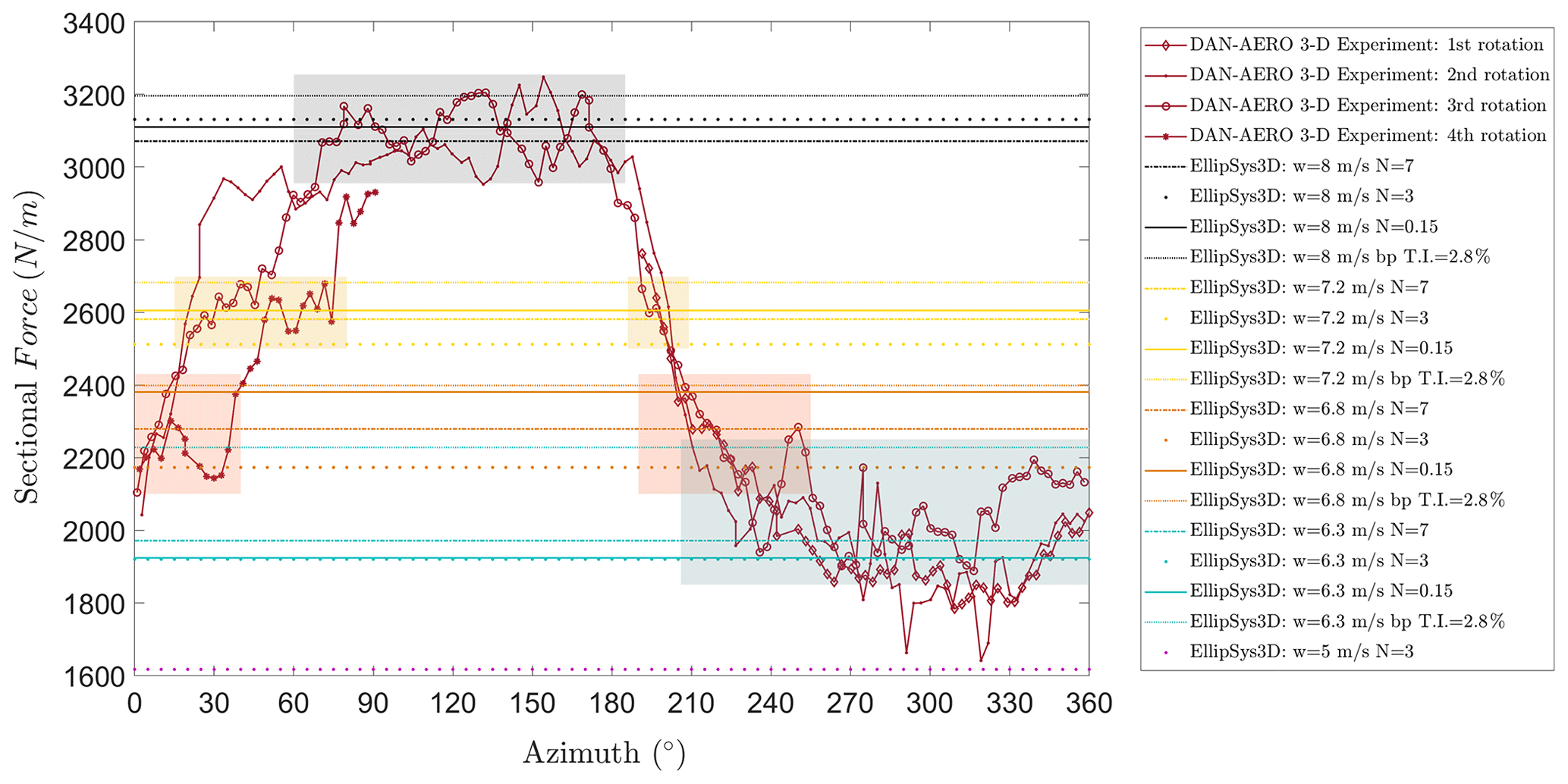
Figure 9Sectional normal force versus azimuth angle from the DAN-AERO experiments compared with EllipSys3D simulations with several inflow cases. (The CFD results are labeled by colors for the different free-stream velocities (w), i.e., black: w=8 m s−1; yellow: w=7.2 m s−1; orange: w=6.8 m s−1; turquoise: w=6.3 m s−1; purple: w=5 m s−1.) The color blocks show the fitted regions from the CFD results with the experiments.
While large-scale vortices contained in the wake of the upstream turbine might mean higher turbulence intensities, there is a also a velocity reduction due to the energy extracted from the wind by the upstream turbine. Therefore, in the wake region, the experimental force shows agreement with the forces obtained from the simulations with a lower inflow velocity (the fitted region is highlighted by the turquoise block). It is also observed from the data that high-wake cases introduce a bigger amount of variation in the sectional force compared to low-wake cases.
It is seen that the experimental force variation for four revolutions is comparable with the numerical results. For further validation, the transition points are also compared for the pressure and the suction sides in Figs. 10 and 11 respectively. Figures 9–11 show the results for the same measurement dataset. Three different turbulence intensity levels are shown in most of the cases to cover several ranges of turbulence intensity levels in the atmosphere.
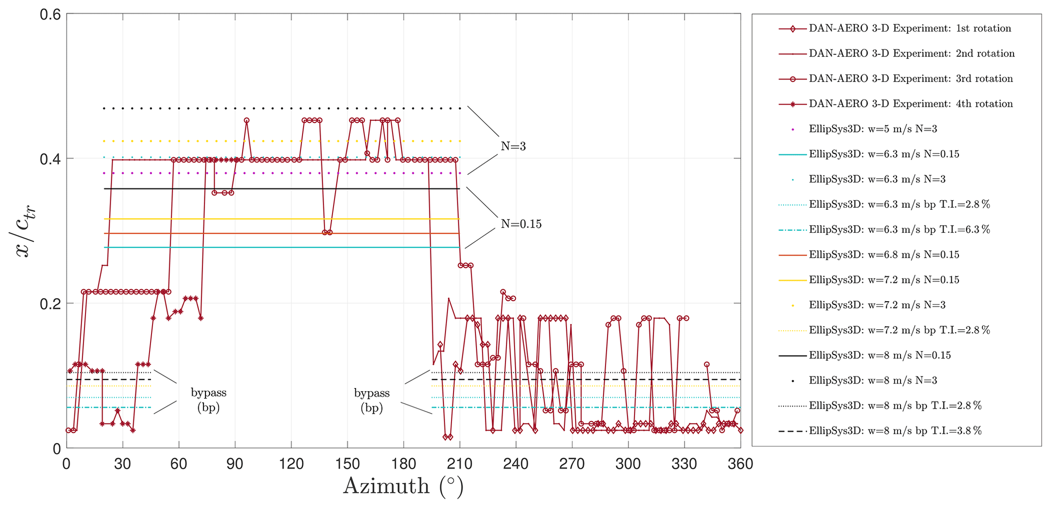
Figure 10Experimentally detected transition points as functions of azimuth angle and EllipSys3D simulation transition results for various different scenarios for the pressure side of the blade section. (The CFD results are labeled by colors for the different free-stream velocities (w), i.e., black: w=8 m s−1; yellow: w=7.2 m s−1; orange: w=6.8 m s−1; turquoise: w=6.3 m s−1; purple: w=5 m s−1.)
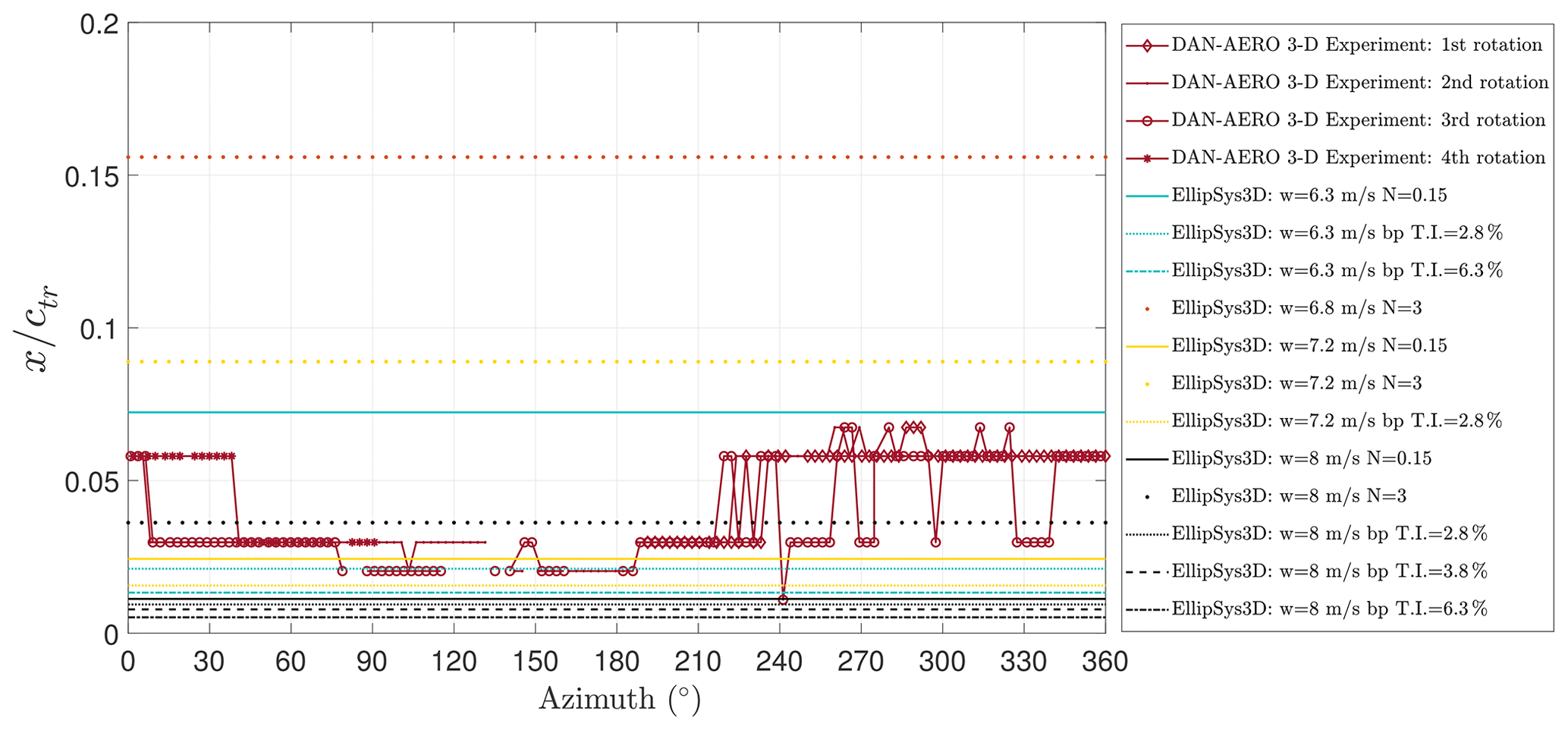
Figure 11Experimentally detected transition points as functions of azimuth angle and EllipSys3D simulation transition results for various different scenarios for the suction side of the blade section. (The CFD results are labeled by colors for the different free-stream velocities (w), i.e., black: w=8 m s−1; yellow: w=7.2 m s−1; orange: w=6.8 m s−1; turquoise: w=6.3 m s−1.)
It is seen from Fig. 10 that the azimuthal angles that correspond to the wake inflow conditions match with the bypass transition results. The main flow condition measured from the meteorological mast is U∞=8 m s−1 and from the pitot tube on the blade %, which corresponds to the N=0.15 with Mack's estimation. The regions where the transition point is around 20 % of the chord is due to the effect of the decreasing AOA by decreasing relative velocity in the wake region. Moreover, the regions where the transition point moves closer to the leading edge, approximately to 3 %, are the indication of the direct effect of the inflow turbulence on the transition point in addition to the decreasing AOA. In those regions, the amplification of the small disturbances is bypassed. Considering the standard deviation of the measurements, EllipSys3D transition results cover most of the scenarios that the turbine is exposed to during rotation.
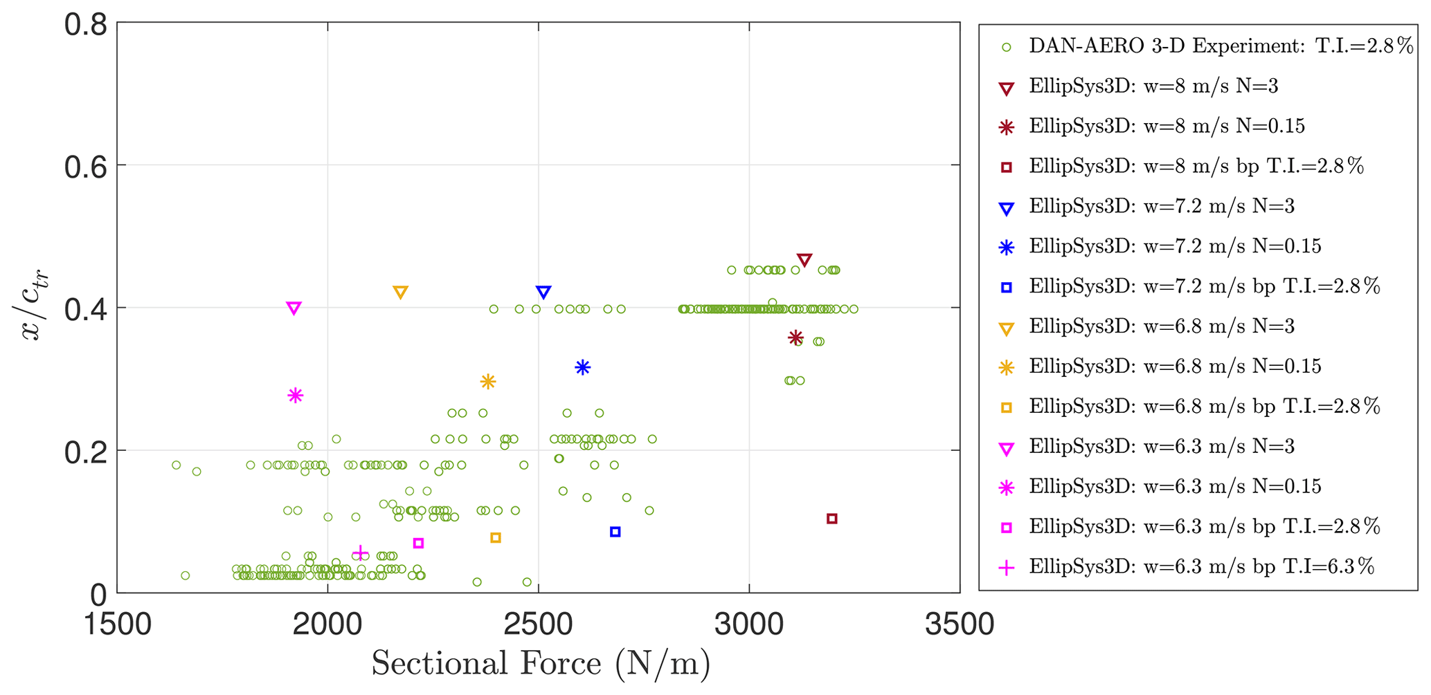
Figure 12Experimentally detected transition points on the pressure side versus sectional normal force over four revolutions compared with the EllipSys3D simulation results.
On the suction side, in Fig. 11, the opposite behavior of the transition point is noticeable with the angle variation. The regions where the transition point is closer to the leading edge correspond to the high-angle regions. The regions under wake at higher azimuthal angles correspond to the decreasing Vrel and AOA (see Fig. 6 – right), which moved the transition point further downstream. In this region on the suction side, although the turbulence intensity is increasing, the individual effect of the increasing AOA is more prominent than the effect of the inflow turbulence itself. However, variations between each rotation are also noticeable, which might be due to the inflow turbulence. It should be noted that although there are rotational changes in the transition point, x∕ctr, on the suction side of the rotor blade section, the detected transition locations are considerably close to the leading edge, so the relative movement is not as prominent as on the pressure side and it is harder to reach a reliable conclusion.
The transition positions from the microphone measurements and the sectional forces derived from the pressure measurements are coupled. x∕ctr on the pressure side as a function of the sectional normal force is presented in Fig. 12. In the same way, the EllipSys3D transition point results are presented as a function of the sectional force obtained from the simulations. Each EllipSys3D transition location-normal force point corresponds to a different simulation setup where the input velocity and the amplification factor for the natural transition model and the turbulence intensity for the bypass transition model are varied. This comparison indicates that the simulation results are in line with the experiments although a considerable scatter is seen.
The pressure coefficient results from the pressure taps and those from the simulations are also compared. In the experiments, four blade sections are equipped with pressure taps, and the current analysis shows the most outward section (next to the microphones) has the highest velocity change with the azimuth compared to the other sections. The pressure coefficient is calculated as follows:
where V∞ is the free-stream velocity measured on the meteorological mast, r is the radial position of the section where the microphones are located, and ω is the rotational speed of the turbine. The pressure coefficient from the experiments is obtained by azimuthal averaging of the pressure measurements from 570 s time data. For comparison, Cp values obtained by averaging through the full rotation are also presented in Fig. 13. Moreover, both EllipSys2D and EllipSys3D results are presented, and DAN-AERO experiments from the wind tunnel measurements (DAN-AERO 2-D) are also included.

Figure 13Pressure coefficient (Cp) comparison of the 2-D and 3-D simulations and the experimental results for an azimuth angle of 0∘ (a), comparison of the 3-D experimental results at a 90∘ azimuth angle with numerical results featuring several free-stream velocities (b), and comparison of 3-D experimental results at a 270∘ azimuth angle with 3-D numerical results for fully turbulent (“ft”), natural, and bypass transition (“bp”) models (c). For each plot, the Cp value obtained by averaging through full rotation is also presented and denoted as “fullrot”.
The Cp value from field experiments for a 0∘ azimuthal angle and for the full rotation is presented in Fig. 13a. The EllipSys3D result, simulated with a free-stream velocity of 7.2 m s−1, fits well with the 3-D experimental results. At this azimuthal position, the AOA values seen in the field experiments vary from 4 to 7.5∘. The 2-D results presented here are for AOA=4 and 5∘, at a Reynolds number of 5 million. Furthermore, the 2-D results for higher angle-of-attack values are also found to be still within the standard deviation of the pressure coefficient from the field experiments. Although there are some bumps on the Cp curve for the 2-D simulations and for both the 2-D and 3-D experiments on the suction side due to the manufactured geometry, there are no visible bumps in the 3-D simulations since the blades were generated with theoretical airfoil sections for the 3-D simulations.
The Cp values obtained from 3-D simulations and experimental Cp value at a 90∘ azimuthal angle are presented in Fig. 13b. EllipSys3D simulations for various free-stream velocities observed during the acquisition time of the pressure measurements fit well with the 3-D experimental results. In Fig. 13c, EllipSys3D results for fully turbulent, natural, and bypass transition are shown for the 270∘ azimuthal position. This is the region where there is wake-affected inflow in this measurement set; therefore numerical results obtained for lower free-stream velocities show agreement with the 3-D experimental results.
In order to have a wider discussion, all the selected measurements from different days in the field experiments with different pitch settings, inflow velocities, and T.I. under both wake and no-wake conditions are gathered and plotted as a function of the AOA. As explained in Sect. 3, for the EllipSys3D results, the effective angle of attack on the blade section is determined by annular averaging of the axial velocity method in order to compare the results with 2-D simulations and experiments. Moreover, the AOA values derived from the force measurements in the 3-D experiments with the detected transition points from the microphone measurements are added to this comparison. The field experiment results contain measurements from 2 different days with two pitch (p) settings of 1.25 and 4.75∘ and both wake and no-wake conditions. These data are binned according to the pitch setting and wake shadow ranges. Transition points as a function of the AOA for both 2-D and 3-D experiments and simulations are shown in Fig. 14. The airfoil tested in the wind tunnel is manufactured identically to the rotor blade section surface geometry. Therefore, possible surface irregularities are also transferred. The reason of the sudden change of the transition point from to −5∘ on the suction side in the 2-D experiments instead of following a gradual pattern as in the EllipSys2D simulations might be due to these irregularities.
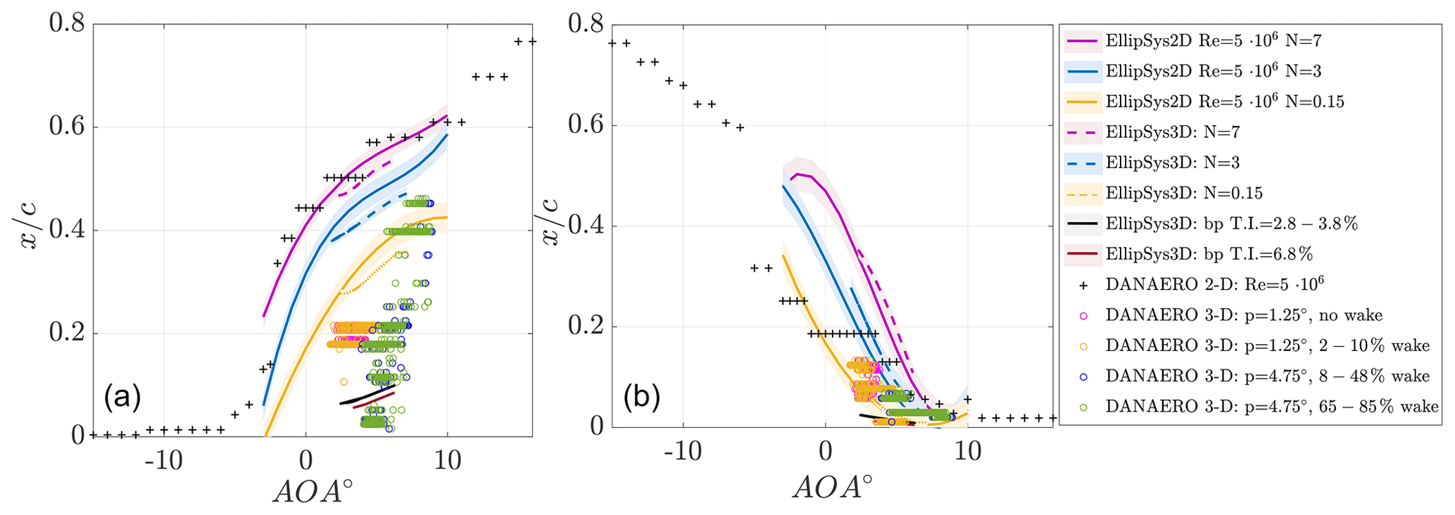
Figure 14Detected transition points from the field and wind tunnel experiments and from the 2-D and 3-D CFD computations for the pressure side (a) and for the suction side (b). (The EllipSys 2-D and 3-D results are presented as a fitted line of the data. Shadows around the lines show the standard deviation of the fit.)
It can be seen from Fig. 14 – left (pressure side) that for the high AOA and high-inflow turbulent cases, the transition locations are scattered around a larger percentage of the chord (from to , approx. 44 % area), which creates a significant effect on the performance of the wind turbine. However, for lower AOA values under no-wake conditions, the transition point does not move more than 10 % along the chord during a revolution. The 2-D simulations with N=7 and the wind tunnel experiments show good agreement on the pressure side. It is seen that there is a significant difference on the pressure side between the 2-D wind tunnel experimental results and 3-D field experiments at several inflow conditions for the same manufactured airfoil geometry. For the high-pitch case (p=4.75∘), at AOA values from 4 to 9∘, the jump in the transition location seen in the 3-D experiments is not visible either in wind tunnel results or in 2-D or 3-D simulations. These changes in the location of transition points during one revolution are represented by the simulations with different N factors for the natural transition model and different T.I. values for the bypass transition model. The bypass transition model fits with the locations close to the leading edge, and this shows that at several azimuthal positions, the transition is bypassed in the field experiments. The natural transition model with N=0.15 and N=3 fits to the positions where the transition locations are found to be at around 40 % of the chord. By combination of the results from the simulations with bypass and natural transition models, the scattered area from the experiments is covered. For the suction side (Fig. 14 – right), the results from the 3-D simulations with natural and bypass transition models cover most of the results from the field experiments. For the low AOA values, and low- and no-wake cases, the transition location movement is within 13 % along the chord in one revolution for the suction side. The more downstream transition locations, seen at low AOA values, fit with the results from the simulations with the natural transition model. This indicates that the natural transition type is also present on the suction side. Moreover, the 2-D and 3-D experimental results show agreement in the high AOA range on the suction side, and the transition locations are in very close proximity of the leading edge in most of the cases.
In this study, the analysis of the field experiments and results from the 3-D CFD simulations are presented to characterize the laminar-turbulent transition behavior of a wind turbine under real atmospheric conditions. The data from high-frequency microphones placed on a wind turbine blade section are analyzed in the time and frequency domains. The transition locations are detected from the standard deviation of the pressure fluctuations, which are integrated between 2 and 7 kHz. The inflow turbulence behavior is obtained from one of the microphones placed close to the leading edge by integrating the spectra from 100 to 300 Hz. The inflow velocity is obtained from meteorological mast measurements and used as an input parameter in the CFD computations. The T.I. for the simulations is obtained from the relative velocity measurement from the pitot tube placed on the blade section.
The field experiment results showed that the transition behavior on the wind turbine blade in real operating conditions differs from the model in the wind tunnel, caused by the influence of the inflow turbulence and the wake from another turbine. These factors change the relative velocity, and thus the effective AOA on the blade section, and, besides, inflow turbulence is observed to have some direct effects on transition.
The effect of the wake is visible from the variation in the detected transition points at each revolution. As the wake-affected rotor area increases, bigger jumps of the transition position are observed during one revolution. At the low- and no-wake cases, each revolution is almost identical, and the transition behavior is mainly governed by the angle-of-attack changes due to the inflow velocity. The angle-of-attack effect on transition is analyzed by comparing results from the two different pitch settings under similar inflow conditions. It is seen that for the pressure side, at low-AOA cases, the transition position is not affected by the variations during a revolution as much as in the high-AOA cases. Changes in AOA are found to be highly correlated with transition locations during a revolution, and the variations among different revolutions are due to the inflow turbulence.
The normal sectional forces from the experiments and simulations are compared in order to quantify the rotational changes of the force and analyze the differences among several revolutions. Moreover, by binning the sectional forces from the experiments by the inflow velocity, the range that is covered by the simulation results obtained with various N numbers for the natural transition and T.I. for the bypass transition is identified. It is seen that the field experiments and the 3-D simulations are comparable.
Furthermore, detected transition positions for the suction and pressure sides from the field experiments are compared with 3-D CFD simulations. It is seen from the experiments that as the inflow fluctuations increase, the transition point moves closer to the leading edge on the pressure side of the blade section. The EllipSys3D bypass transition model pressure side predictions are in good agreement with the experimental cases in conditions of high inflow turbulence at the azimuthal positions where the turbine is under the wake of an upstream turbine. On the other hand, the experimental result from the other azimuthal positions fit to the results obtained with the natural transition model. At these positions, the free-stream velocities at different height levels of the ABL are matched with the azimuthal positions of the blade section. Comparing many datasets from different days, it is seen that for high-AOA and high-wake cases, the movement of the transition point covers up to 44 % of the chord on the pressure side in a single revolution, a value that drops to 5 % at low AOA and for no-wake cases. On the suction side, changes in the transition position are also observable, and the field and wind tunnel experiments agree in the high-AOA range. It is seen that, on the suction side, the effect of AOA is more prominent than the direct effect of the turbulence intensity, though it is not easy to reach a conclusion as the transition positions are in very close proximity to the leading edge (within %–13 %). Therefore, at these physical conditions, the suction side is not suited to distinguish the type of the transition mechanism. It is visible from the pressure coefficient results that for an azimuth angle of 270∘, where there is a wake from an upstream turbine for the presented case, the experiments fit with the low-velocity 3-D simulation results for natural and bypass transition models. On the other hand, a 90∘ azimuthal position corresponds to a high-AOA region in the field experiments, a suction peak increase is observed, and the EllipSys3D results that are simulated for the velocities during 10 min acquisition time fit with the experiments. For a 0∘ azimuth, it is seen that 2-D simulation and experimental results are within the standard deviation of 3-D experiments. The pressure coefficient results also show the surface bumps on the suction side that could have been one of the factors affecting transition.
It is seen that the eN semiempirical transition model and bypass transition model in EllipSys3D can be used for high-Reynolds-number flows (Re=5 million) in real atmospheric conditions. Using both models can cover the range of transition positions that is seen in the field experiments with a relevant choice of the amplification factors and T.I. values.
Several inflow scenarios are simulated separately in EllipSys3D as it is hard to control high turbulence in the wake region and handling varying N factor and T.I. values in a single simulation. Simulations with more inflow characterization can be studied in the future in order to simulate the real inflow conditions from the experiments. Moreover, detailed characterization of the inflow turbulence measured on the blade with high-sampling-frequency instruments in field experiments is needed to separate relevant frequencies that affect boundary layer transition. By more field experiments and high-resolution simulations, laminar-turbulent transition predictions can evolve and eventually contribute to the aerodynamic prediction and the design of the wind turbine blades.
Data are available upon request to the corresponding author.
The literature review, the experimental data selection, processing and transition detection, the majority of the manuscript writing, mesh generation for EllipSys2D simulations, the EllipSys2D and 3-D simulations, and postprocessing of the simulations and comparisons of the results from the experiments and the simulations were conducted by ÖSÖ. The DAN-AERO 3-D and 2-D experimental data and the guidance for the experimental data were provided by HAM. The CFD mesh for the EllipSys3D computations and technical and theoretical guidance in CFD computations were provided by NNS. The corrections in the manuscript and technical advice were provided by JNS. All authors took part in writing and editing the paper.
The authors declare that they have no conflict of interest.
This paper was edited by Michael Muskulus and reviewed by two anonymous referees.
Abu-Ghannam, B. and Shaw, R.: Natural transition of boundary layers – the effects of turbulence, pressure gradient, and flow history, J. Mech. Eng. Sci., 22, 213–228, 1980. a
Arnal, D., Gasparian, G., and Salinas, H.: Recent Advances in Theoretical Methods for Laminar-Turbulent Transition Prediction, in: 36th AIAA Aerospace Sciences Meeting and Exhibit, 12–15 January 1998, Reno, NV, USA, https://doi.org/10.2514/6.1998-223, 1998. a
Bak, C., Aagaard Madsen, H., Schmidt Paulsen, U., Gaunaa, M., Fuglsang, P., Romblad, J., Olesen, N., Enevoldsen, P., Laursen, J., and Jensen, L.: DAN-AERO MW: Detailed aerodynamic measurements on a full scale MW wind turbine, in: EWEC 2010 Proceedings online, European Wind Energy Association (EWEA), Warsaw, 2010. a
Bertolotti, F. P., Herbert, T., and Spalart, P. R.: Linear and nonlinear stability of the Blasius boundary layer, J. Fluid Mech., 242, 441–474, https://doi.org/10.1017/S0022112092002453, 1992. a
Biau, D., Arnal, D., and Vermeersch, O.: A transition prediction model for boundary layers subjected to free-stream turbulence, Aerospace Sci. Technol., 11, 370–375, 2007. a
Boorsma, K., Schepers, J. G., Gomez-Iradi, S., Herraez, I., Lutz, T., Weihing, P., Oggiano, L., Pirrung, G., Madsen, H. A., Shen, W. Z., and Rahimi, H.: Final report of IEA wind task 29 Mexnext (Phase 3), Wind Energy, available at: https://scholar.google.com.tr/scholar?cluster=6869701785559421965&hl=en&as_sdt=0,5 (last access: October 2020), 2018. a
Chaviaropoulos, P. K., Sieros, G., Prospathopoulos, J. M., Diakakis, K., and Voutsinas, S. G.: Design and CFD-based Performance Verification of a Family of Low-Lift Airfoils, EAWE, Paris, 2015. a
Chen, K. K. and Thyson, N. A.: Extension of Emmons' spot theory to flows on blunt bodies, AIAA J., 9, 821–825, 1971. a
Davis, M., Reed, H., Youngren, H., Smith, B., and Bender, E.: Transition Prediction Method Review Summary for the Rapid Assessment Tool for Transition Prediction (RATTraP), US Air Force Research Lab. Technical Rep. VA-WP-TR-2005-3130, Wright–Patterson AFB, OH, 2005. a
Dhawan, S. and Narasimha, R.: Some properties of boundary layer flow during the transition from laminar to turbulent motion, J. Fluid Mech., 3, 418–436, 1958. a
Diakakis, K., Papadakis, G., and Voutsinas, S. G.: Assessment of transition modeling for high Reynolds flows, Aerospace Sci. Tech., 85, 416–428, 2019. a
Dini, P., Selig, M. S., and Maughmer, M. D.: Simplified Linear Stability Transition Prediction Method for Separated Boundary Layers, AIAA J., 30, 1953–1961, https://doi.org/10.2514/3.11165, 1992. a
Drela, M. and Giles, M. B.: Viscous-inviscid analysis of transonic and low Reynolds number airfoils, AIAA J., 25, 1347–1355, 1987. a, b
Emmons, H.: The laminar-turbulent transition in a boundary layer – Part I, J. Aeronaut. Sci., 18, 490–498, 1951. a
Eppler, R.: Practical calculation of laminar and turbulent bled-off boundary layers, Report number NASA-TM-75328, NASA Technical Memorandum, NASA, Washington, D.C., 1978. a
FieldView: FieldView Reference Manual, Intelligent Light, Rutherford, NJ, 2017. a
Gleyzes, C., Cousteix, J., and Bonnet, J. L.: A Calculation Method of Leading Edge Separation Bubbles, in: Numerical and Physical Aspects of Aerodynamic Flows II, edited by: Cebeci, T., Springer, Berlin, Heidelberg, 1983. a
Hansen, M. O., Sørensen, N. N., and Michelsen, J.: Extraction of lift, drag and angle of attack from computed 3-D viscous flow around a rotating blade, in: 1997 European Wind Energy Conference, Irish Wind Energy Association, Slane, 499–502, 1997. a
Herbert, T.: Parabolized stability equations, Annu. Rev. Fluid Mech., 29, 245–283, 1997. a
Hernandez, G. G. M., Sørensen, J. N., and Shen, W. Z.: Laminar-turbulent transition on wind turbines, DTU Mechanical Engineering, Kgs. Lyngby, 2012. a
Johansen, J. and Sørensen, N. N.: Aerofoil characteristics from 3D CFD rotor computations, Wind Energy, 7, 283–294, https://doi.org/10.1002/we.127, 2004. a
Joseph, L. A., Borgoltz, A., and Devenport, W.: Infrared thermography for detection of laminar–turbulent transition in low-speed wind tunnel testing, Exp. Fluids, 57, 57–77, 2016. a
Krumbein, A.: Application of Transition Prediction, in: MEGADESIGN and MegaOpt –German Initiatives for Aerodynamic Simulation and Optimization in Aircraft Design, edited by: Kroll, N., Schwamborn, D., Becker, K., Rieger, H., and Thiele, F., Springer, Berlin, Heidelberg, 107–120, 2009. a
Kümmerer, H.: Numerische Untersuchungen zur Stabilität ebener laminarer Grenzschichtströmungen, PhD thesis, 1973. a
Langtry, R. B.: A correlation-based transition model using local variables for unstructured parallelized CFD codes, https://doi.org/10.18419/OPUS-1705, 2006. a
Larsen, T. and Hansen, A.: How 2 HAWC2, the user's manual, Denmark, Risoe-R-1597, Forskningscenter, Risoe, 2007. a
Lobo, B., Boorsma, K., and Schaffarczyk, A.: Investigation into Boundary Layer Transition on the MEXICO Blade, J. Phys.: Conf. Ser., 1037, 052020, https://doi.org/10.1088/1742-6596/1037/5/052020, 2018. a
Mack, L. M.: Transition and Laminar Instability, No. NASA-CP-153203, NASA Jet Propulsion Laboratory, California, 1977. a
Madsen, H. A., Bak, C., Paulsen, U. S., Gaunaa, M., Fuglsang, P., Romblad, J., Olesen, N., P., E., Laursen, J., and Jensen, L.: The DANAERO MW Experiments, Tech. Rep. No. Risø-R-1726(EN), Danmarks Tekniske Universitet, Risø Nationallaboratoriet for Bæredygtig Energi, Risø, 2010. a, b
Madsen, H. A.,Özçakmak,Ö. S., Bak, C., Troldborg, N., Sørensen, N. N., and Sørensen, J. N.: Transition characteristics measured on a 2 MW 80 m diameter wind turbine rotor in comparison with transition data from wind tunnel measurements, in: AIAA Scitech 2019 Forum, January 2019 San Diego, California, https://doi.org/10.2514/6.2019-0801, 2019a. a, b
Madsen, M. H. A., Zahle, F., Sørensen, N. N., and Martins, J. R. R. A.: Multipoint high-fidelity CFD-based aerodynamic shape optimization of a 10 MW wind turbine, Wind Energ. Sci., 4, 163–192, https://doi.org/10.5194/wes-4-163-2019, 2019b. a
Mayle, R.: A theory for predicting the turbulent-spot production rate, in: ASME 1998 International Gas Turbine and Aeroengine Congress and Exhibition, V001T01A071, American Society of Mechanical Engineers, New York, 1998. a
Menter, F.: Zonal two equation kw turbulence models for aerodynamic flows, in: 23rd fluid dynamics, plasmadynamics, and lasers conference, 6–9 July 1993, Orlando, FL, USA, p. 2906, 1993. a
Menter, F. R., Langtry, R. B., Likki, S., Suzen, Y., Huang, P., and Völker, S.: A correlation-based transition model using local variables – part II: model formulation, J. Turbomach., 128, 413–422, 2006. a
Michel, R.: Etude de la Transition sur les Profiles d'Aile; Etablissement d'un Critére de Determination de Point de Transition et Calcul de la Trainee de Profile Incompressible, ONERA Report 1/1578A, 1951. a
Michelsen, J. A.: Basis3D-a platform for development of multiblock PDE solvers, Tech. rep., Technical Report AFM 92-05, Technical University of Denmark, Denmark, 1992. a
Michelsen, J. A.: Block structured Multigrid solution of 2D and 3D elliptic PDE's, Department of Fluid Mechanics, Technical University of Denmark, Denmark, 1994. a
Michelsen, J. A.: Beregning af laminar-turbulentomslag i 2D og 3D, in: vol. Risø-R-1349(DA), Technical University of Denmark, Risø, 37–47, 2002. a, b
Morkovin, M. V.: Critical evaluation of transition from laminar to turbulent shear layers with emphasis on hypersonically traveling bodies, Tech. rep., Martin Marietta Corp Baltimore Md Research Inst. for Advanced Studies, Air Force Flight Dynamics Laboratory, Ohio, 1969. a
Morkovin, M. V.: Bypass Transition to Turbulence and Research desiderata, NASA, Lewis Research Center Transition in Turbines, 161–204, 1985. a
Özçakmak,Ö. S., Madsen, H. A., Sørensen, N., Sørensen, J. N., Fischer, A., and Bak, C.: Inflow Turbulence and Leading Edge Roughness Effects on Laminar-Turbulent Transition on NACA 63-418 Airfoil, J. Phys.: Conf. Ser., 1037, 022005, https://doi.org/10.1088/1742-6596/1037/2/022005, 2018. a
Özçakmak,Ö. S., Sørensen, N. N., Madsen, H. A., and Sørensen, J. N.: Laminar-turbulent transition detection on airfoils by high-frequency microphone measurements, Wind Energy, 22, 1356–1370, https://doi.org/10.1002/we.2361, 2019. a, b, c, d, e
Patankar, S. V.: Numerical heat transfer and fluid flow, Hemisphere Publ. Corp., New York, 1980. a
Patankar, S. V. and Spalding, D. B.: A calculation procedure for heat, mass and momentum transfer in three-dimensional parabolic flows, in: Numerical Prediction of Flow, Heat Transfer, Turbulence and Combustion, Imprint, Pergamon, 54–73, 1983. a
Reichstein, T., Schaffarczyk, A. P., Dollinger, C., Balaresque, N., Schülein, E., Jauch, C., and Fischer, A.: Investigation of Laminar–Turbulent Transition on a Rotating Wind-Turbine Blade of Multimegawatt Class with Thermography and Microphone Array, Energies, 12, 2102, https://doi.org/10.3390/en12112102, 2019. a
Reshotko, E.: Stability theory as a guide to the evaluation of transition data., AIAA J., 7, 1086–1091, https://doi.org/10.2514/3.5279, 1969. a
Reza, T. Z. and Amir, K.: Prediction of boundary layer transition based on modeling of laminar fluctuations using RANS approach, Chin. J. Aeronaut., 22, 113–120, 2009. a
Rhie, C. and Chow, W.: A numerical study of the turbulent flow past an isolated airfoil with trailing edge separation, in: 3rd Joint Thermophysics, a
Schaffarczyk, A. P., Schwab, D., and Breuer, M.: Experimental Detection of Laminar-Turbulent Transition on a Rotating Wind Turbine Blade in the Free Atmosphere, Wind Energy, 20, 211–220, https://doi.org/10.1002/we.2001, 2017. a
Schaffarczyk, A. P., Boisard, R., Boorsma, K., Dose, B., Lienard, C., Lutz, T., Madsen, H. Å., Rahimi, H., Reichstein, T., Schepers, G., Sørensen, N., Stoevesandt, B., and Weihing, P.: Comparison of 3D transitional CFD simulations for rotating wind turbine wings with measurements, J. Phys.: Conf. Ser., 1037, 022012, https://doi.org/10.1088/1742-6596/1037/2/022012, 2018. a
Schepers, J. and Snel, H.: Model experiments in controlled conditions, ECN Report ECN-E-07-042, ECN, the Netherlands, 2007. a
Schwab, D., Ingwersen, S., Schaffarczyk, A. P., and Breuer, M.: Aerodynamic Boundary Layer Investigation on a Wind Turbine Blade under Real Conditions, in: Wind Energy – Impact of Turbulence, edited by: Hölling, M., Peinke, J., and Ivanell, S., Springer, Berlin, Heidelberg, 203–208, 2014. a
Smith, A. and Gamberoni, N.: Transition, pressure gradient, and stability theory, Report no. es. 26388, Douglas Aircraft Co, Inc., El Segundo, CA, 1956. a
Sørensen, N. N.: General Purpose Flow Solver Applied to Flow Over Hills, PhD thesis, Risø National Laboratory, Risø, 1995. a
Sørensen, N. N.: HypGrid2D. A 2-d mesh generator, Tech. rep., Risø National Laboratory, Risø, 1998. a
Sørensen, N. N.: CFD modelling of laminar-turbulent transition for airfoils and rotors using the γ-model, Wind Energy, 12, 715–733, https://doi.org/10.1002/we.325, 2009. a, b
Sørensen, N. N., Bechmann, A., and Zahle, F.: 3D CFD computations of transitional flows using DES and a correlation based transition model, Wind Energy, 14, 77–90, 2011. a
Sørensen, N. N., Zahle, F., and Michelsen, J. A.: Prediction of airfoil performance at high Reynolds numbers EFMC, Sound/Visual production (digital), Kgs. Lyngby, Denmark, 2014. a
Stock, H. and Degenhart, E.: A simplified e exp n method for transition prediction in two-dimensional, incompressible boundary layers, Z. Flugwiss. Weltraumforsch., 13, 16–30, 1989. a
Stock, H. W. and Haase, W.: Feasibility Study of e Transition Prediction in Navier–Stokes Methods for Airfoils, AIAA J., 37, 1187–1196, 1999. a
Suder, K. L., Obrien, J. E., and Reshotko, E.: Experimental study of bypass transition in a boundary layer, MsT, NASA Lewis Research Center, Case Western Reserve Univ., Cleveland, Ohio, p. 20, 1988. a
Suzen, Y. and Huang, P.: Modeling of flow transition using an intermittency transport equation, J. Fluids Eng., 122, 273–284, 2000. a
Suzen, Y., Xiong, G., and Huang, P.: Predictions of transitional flows in low-pressure turbines using intermittency transport equation, AIAA J., 40, 254–266, 2002. a, b
Troldborg, N., Bak, C., Aa., M. H., and Witold, S.: DANAERO MW: Final Report, Tech. Rep. No. 0027(EN), DTU Wind Energy, Risø, 2013. a, b
Van Ingen, J. L.: A Suggested Semi-Empirical Method for The Calculation of the Boundary Layer Transition Region, Tech. Rep. No. V.T.H.-74, Delft University of Technology, Delft, 1956. a
Von Kármán, T.: Uber laminare und turbulente Reibung, Z. Angew. Math. Mech., 1, 233–252, 1921. a
Walters, D. K. and Leylek, J. H.: A new model for boundary layer transition using a single-point RANS approach, J. Turbomach., 126, 193–202, 2004. a
Wazzan, A., Okamura, T., and Smith, A.: Spatial and temporal stability charts for the Falkner–Skan boundary-layer profiles, Tech. rep., McDonnell Douglas Astronautics Co-Hb, Huntington Beach, CA, 1968. a
Welch, P.: The use of fast Fourier transform for the estimation of power spectra: a method based on time averaging over short, modified periodograms, IEEE T. Audio Electroacoust., 15, 70–73, 1967. a
Yilmaz, Ö. C., Pires, O., Munduate, X., Sørensen, N. N., Reichstein, T., Schaffarczyk, P., Diakakis, K., Papadakis, G., Daniele, E., Schwarz, M., Lutz, T., and Prieto, R.: Summary of the blind test campaign to predict the high Reynolds number performance of DU00-W-210 airfoil, in: 35th Wind Energy Symposium, 9–13 January 2017, Grapevine, Texas, p. 0915, 2017. a