Automatic controller tuning using a zeroth-order optimization algorithm

We develop an automated controller tuning procedure for wind turbines that uses the results of nonlinear, aeroelastic simulations to arrive at an optimal solution. Using a zeroth-order optimization algorithm, simulations using controllers with randomly generated parameters are used to estimate the gradient and converge to an optimal set of those parameters. We use kriging to visualize the design space and estimate the uncertainty, providing a level of confidence in the result.

The procedure is applied to three problems in wind turbine control. First, the below-rated torque control is optimized for power capture. Next, the parameters of a proportional–integral blade pitch controller are optimized to minimize structural loads with a constraint on the maximum generator speed; the procedure is tested on rotors from 40 to 400 m in diameter and compared with the results of a grid search optimization. Finally, we present an algorithm that uses a series of parameter optimizations to tune the lookup table for the minimum pitch setting of the above-rated pitch controller, considering peak loads and power capture. Using experience gained from the applications, we present a generalized design procedure and guidelines for implementing similar automated controller tuning tasks.

1 Introduction

In this article, we present a data-driven, simulation-based optimization procedure for tuning wind turbine controllers using measures that are directly related to component design. Controller tuning influences the power capture and structural loading on wind turbines, which are directly related to the cost of the wind energy generated. At the same time, different turbine models require different control parameters. As rotor designs are iterated upon and also customized, e.g., with larger towers, tip extensions, or for site-specific turbulence, an updated (and ideally optimized) controller is required for component design and cost specification. Given the aeroelastic turbine model, the algorithm presented in this article automatically finds the optimized parameters of the predefined control architecture, reducing the effort required of the control designer.

The wind turbine control tuning can be automated, but design choices for the various parameters often require expert knowledge of the controller and turbine operation. An automated procedure to determine these choices could reduce the design cycle time of a manufacturer's research and development process or aid researchers in other disciplines of wind engineering that require a well-tuned controller without worrying about its finer details. Several control parameters are directly related to the performance of the turbine and must be tuned for each design iteration or model update. The simplest method to determine these design choices using simulation results is to exhaustively search the design space and then make an educated design choice of the parameter. However, exhaustive search may become computationally intractable for fine discretizations of the search space; on the other hand, coarse discretizations may lead to suboptimal design choices.

A systematic, simulation-based parameter search of the pitch control gains for generator speed control was first published in Hand and Balas (2000). On a single turbine, turbulent simulations were used to sample and visualize the design space against competing design measures: generator speed regulation versus blade pitch actuation. A similar data processing flow was used in Hansen et al. (2005) while the problem was formulated in a numerical optimization framework for structural load reduction; the authors concluded that a good initial guess was only marginally worse than the optimized result and that the effort required to set up the optimization procedure was not profitable for the benefit in structural loading. Shortly thereafter, an adaptive control framework was found to be beneficial for reconciling plant–model mismatches in field testing, especially for control parameters that affect power production (Johnson et al., 2006), where even small benefits are profitable to the operator.

As the wind industry has matured and computational cost has decreased, wind turbine design increasingly relies on simulation of power capture and structural loads for design analysis. As a result, system engineering tools for wind turbine design have been developed and refined, leading to updated efforts in automated controller development, with the aim of deploying tuning methods for many different turbines. One approach is to use a model-based control scheme in order to limit the control tuning effort (Bottasso et al., 2012). Model-based pitch (Hansen et al., 2005) and torque (Johnson et al., 2006) controllers usually result in functioning controllers but require rules of thumb to determine the closed-loop characteristics and can be inaccurate when there are uncertainties in the model.

A scalar cost function was presented in Tibaldi et al. (2014) using measures that are directly related to wind turbine component design, like peak and fatigue loads. The cost function included terms for each turbine part, with factors to capture its relative cost to the turbine. Using measures directly related to the component design, like fatigue and extreme loads in turbulent simulations, is ideal because it most accurately reflects the eventual component design, but these simulations require more detailed and computationally expensive methods to generate the measures.

Simulation-based optimization has been used to solve these problems, where solving for the value of the cost function is expensive compared to the optimization procedure. One approach to solving these types of problems is using response surface methodology (RSM) (Fu, 2014). RSM was originally developed for experimental design (Box and Wilson, 1951) but has increasingly been used with simulation information; it works by fitting a cost function to the simulation results, finding the local gradient of the fit, and optimizing the fitted cost function. The question of how to sample the parameter space remains an open question. Samples can be generated using a grid search or random sampling. An example in the wind energy community by Moustakis et al. (2019) samples the parameter space based on a cost function that considers both where the cost is expected to be optimal and also where it is unknown. Our approach to sampling the parameter space is based on stochastic approximation or “zeroth-order optimization,” which uses the sampled cost function to estimate the local gradient and then optimizes the function with proven convergence results (Ghadimi and Lan, 2013). Other optimization algorithms require an analytical model; the proposed method relies on functional evaluations (e.g., simulation data) and does not require a model to compute gradient information. In one of the original stochastic approximations methods (Kiefer and Wolfowitz, 1952), each dimension of the decision variable is perturbed and a finite-difference method is used to approximate the gradient. Multipoint methods were developed for higher-dimensional cases, where the decision variable can be perturbed in a direction containing multiple dimensions and the directional derivative is used to estimate the gradient (Duchi et al., 2015). If multiple directions are randomly sampled using a normal Gaussian distribution and then averaged to find the directional derivative, it is known as Gaussian smoothing, which has been shown to improve convergence rates (Hajinezhad et al., 2017).

We use a Gaussian smoothing approach to generate samples, estimate the gradient, and identify a (possibly local) minimum point. Then we use the samples to visualize the design space and provide a level of confidence in the result. Previous work in controller optimization usually only provides the cost function and goals of the optimization, whereas this work explicitly details the method for determining the sample simulations and how their results are used to iterate on control designs.

Instead of using cost functions directly related to overall wind turbine performance, our work solves specific wind turbine control problems that are related to the cost of energy. First, the optimization procedure is demonstrated on below-rated torque control to increase power capture. Next, the pitch control parameters for above-rated pitch control are optimized to reduce fatigue or extreme loads on the tower or blades with a maximum generator speed constraint. Finally, the minimum pitch setting of the pitch controller is optimized in a series of parameter optimizations aimed at reducing peak blade loads.

This article is organized as follows. The optimization algorithm and visualization method are presented in Sect. 2. Applications of the algorithm for wind turbine control tuning are presented in Sect. 3, followed by a generalization of the design procedure and guidelines for parameter selection in Sect. 4. Conclusions are presented in Sect. 5, and the generalized wind turbine controller that is tuned in Sect. 3 is described in Appendix A.

Mathematical notation

Superscript notation will be used to index the stage r of the zeroth-order optimization algorithm: e.g., z^r. Additionally, F^T is the transpose of F. If the power of any value is computed, the base will appear in parentheses: e.g., (γ)^r.

2 Method: zeroth-order optimization

The zeroth-order optimization algorithm uses J random samples near the current iteration to estimate a gradient. Then, a typical first-order method ensues: using the estimated gradient, the descent direction and step size are chosen to produce the next iterate. The process is repeated for a number of stages N_stage until convergence is observed. Using the cost function samples, an estimation of the design space is generated to visually verify the results. In each control tuning example presented in this article, the following unconstrained optimization problem is solved:

$$\begin{array}{}\text{(1)}& \begin{array}{c}\min \\ \mathit{z}\in \mathcal{X}\end{array}\mathcal{C}\left(\mathit{z}\right),\end{array}$$

where $\mathit{z}\in \mathcal{X}\subset {\mathbb{R}}^M$ is the M-dimensional parameter or vector of control parameters, constrained to be in a set 𝒳 that is convex and compact; $\mathcal{C}:{\mathbb{R}}^M\to \mathbb{R}$ is the cost function, which we assume is differentiable, bounded from below, and its gradient is Lipschitz (Ghadimi and Lan, 2013). However, we only have access to the cost function via samples of potentially noisy simulation results.

2.1 Generating samples

The algorithm begins with an initial guess z¹. During each stage $r=\mathrm{1},\mathrm{2},\mathrm{\dots },N_{\mathrm{stage}}$, the gradient is estimated by randomly sampling the design space. During each stage, sample directions ${\mathit{\varphi }}_j^r\in {\mathbb{R}}^M,j=\mathrm{1},\mathrm{2},\mathrm{\cdots },J$ are parameters drawn from a random distribution. In the most general case, a standard normal distribution is used for each dimension and the vectors are normalized to have a unit magnitude; this results in a uniformly random distribution of directions in M-dimensions (Hajinezhad et al., 2017). In this article, we focus on one- and two-dimensional parameter optimizations and will make changes to the generation of the sample directions ${\mathit{\varphi }}_j^r$ to ensure an even distribution for a small number of samples.

A search sample ${\mathit{z}}_j^r$ in stage r is generated according to

$$\begin{array}{}\text{(2)}& {\mathit{z}}_j^r={\mathit{z}}^r+\mathit{\mu }{\mathit{\varphi }}_j^r,\end{array}$$

where μ is a smoothing parameter that determines the amount of space over which the parameter space is searched. A large value for μ helps to estimate the value of the cost function over a larger area (Sect. 2.6), but smaller values of μ tend to result in more accurate convergence.

The number of stages and samples per stage must also be chosen by the designer. A large number of samples per stage gives the best estimate for the gradient but requires more simulations. During the development of this work, it was found that a smaller number of samples per stage and more stages resulted in better convergence using the same total number of simulations (e.g., in Sect. 3.2.2).

2.2 Gradient estimation

At each stage r, the cost 𝒞(z) is computed via simulation at each search sample and used to estimate the gradient

$$\begin{array}{}\text{(3)}& \stackrel{\mathrm{‾}}{\mathit{G}}\left({\mathit{z}}^r\right)={\displaystyle \frac{\mathrm{1}}{J}}\sum _{j=\mathrm{1}}^J{\displaystyle \frac{\mathcal{C}({\mathit{z}}^r+\mathit{\mu }{\mathit{\varphi }}_j^r)-\mathcal{C}\left({\mathit{z}}^r\right)}{\mathit{\mu }}}{\mathit{\varphi }}_j^r.\end{array}$$

Note that Eq. (3) differs from a finite-difference method of estimating the gradient, where the factor ${\mathit{\varphi }}_j^r$ would be in the denominator. Because there is uncertainty expected in the computed cost, small perturbations ($\mathit{\mu }{\mathit{\varphi }}_j^r$) and a nonsmooth cost function 𝒞(z) could result in noisy gradients. The gradient estimator in Eq. (3) is referred to as the random direction gradient estimator (Fu, 2014, p. 110) and maintains the convergence criterion when used in a first-order algorithm (Hajinezhad et al., 2017).

2.3 Determine descent direction

From the estimated gradient, the possible descent direction is computed:

$$\begin{array}{}\text{(4)}& {\mathit{d}}_r=-\mathbf{D}\stackrel{\mathrm{‾}}{\mathit{G}}\left({\mathit{z}}^r\right),\end{array}$$

where a diagonal matrix D of positive scalars is used to relatively increase d_r in the directions where the sensitivities of the cost function to parameter changes are smallest, providing a diagonal approximation to Newton's method and improving convergence rates (Bertsekas, 1999), which leads to the following stage gain:

$$\begin{array}{}\text{(5)}& {\mathit{z}}^{r+\mathrm{1}}={\mathrm{Proj}}_{(\mathrm{1}-\mathit{\rho })\mathcal{X}}\mathit{\{}{\mathit{z}}^r+{\mathit{d}}_r\mathit{\alpha }\mathit{\}},\end{array}$$

where α is the step size and ${\mathrm{Proj}}_{\mathcal{X}}\mathit{\left\{}\mathit{y}\mathit{\right\}}:=\arg {\min }_{\mathit{x}\in \mathcal{X}}\Vert \mathit{x}-\mathit{y}{\Vert }_{\mathrm{2}}^{\mathrm{2}}$ finds the closest point within the parameter bounds 𝒳, offset with ρ=μ so that search samples in the next stage can be generated within the parameter bounds. The algorithm described in Eqs. (2)–(5) is proven to converge to a ball centered around an optimal solution (Hajinezhad et al., 2017). Next, we describe two adjustments to the original algorithm that improve performance when used in the control tuning applications presented in this article.

2.4 Adjustment 1: decreasing step size and line search

A decreasing step size rule ensures convergence and a line search is used so that the cost function does not increase in successive iterations. After choosing a base step size α₀, the cost of test samples

$$\begin{array}{}\text{(6)}& {\mathit{z}}_{a,k}^r={\mathrm{Proj}}_{(\mathrm{1}-\mathit{\rho })\mathcal{X}}\mathit{\{}{\mathit{z}}^r+{\mathit{d}}_r{\mathit{\alpha }}_k\mathit{\}}\end{array}$$

are evaluated (through simulation) along the descent direction, where the step size

$$\begin{array}{}\text{(7)}& {\mathit{\alpha }}_k={\mathit{\alpha }}_{\mathrm{0}}(\mathit{\beta }{)}^{k-\mathrm{1}}\end{array}$$

decreases for a number of iterations k≤k_max. An upper limit k_max on the number of step size samples is chosen to cap the number of simulations that may be performed along directions that could increase the cost function. To ensure that the cost function is nonincreasing during each iteration, the Armijo rule for step size is used (Boyd and Vandenberghe, 2004):

$$\begin{array}{}\text{(8)}& \mathcal{C}\left({\mathit{z}}^r\right)-\mathcal{C}\left({\mathit{z}}_{a,k}^r\right)>-\mathit{\sigma }{\mathit{\alpha }}_k{\stackrel{\mathrm{‾}}{\mathit{G}}}^{\mathrm{T}}{\mathit{d}}_r>\mathrm{0},\end{array}$$

where, for all examples in the following section, σ=0.05 is chosen, a conservative value that only requires a small decrease in the cost function.

2.5 Adjustment 2: resetting parameter update

Once an adequate step size is found, the parameter z is updated using

$$\begin{array}{}\text{(9)}& {\mathit{z}}^{r+\mathrm{1}}={\mathrm{Proj}}_{(\mathrm{1}-\mathit{\rho })\mathcal{X}}\mathit{\{}{\mathit{z}}^r+{\mathit{d}}_r{\mathit{\alpha }}_k\mathit{\}},\end{array}$$

which is the ${\mathit{z}}_{a,k}^r$ in Eq. (6) with the first k that satisfies Eq. (8); since this value has already been computed, the simulation for determining 𝒞(z^r+1) does not need to be performed.

If the maximum number of step size simulations (k=k_max) is performed and the step size rule in Eq. (8) is not satisfied, the next iteration of the parameter z is chosen as

$$\begin{array}{}\text{(10)}& {\mathit{z}}^{r+\mathrm{1}}=\underset{\mathit{z}\in \mathcal{X}}{\mathrm{argmin}}\mathit{C}\left(r\right),\end{array}$$

where C(r) is the enumeration of the cost function at all stage samples z^r, all search samples ${\mathit{z}}_{\mathbf{j}}^{\mathbf{r}}$, and all step size samples ${\mathit{z}}_{a,\mathbf{k}}^{\mathbf{r}}$ within the parameter bounds defined by 𝒳, up until the current stage r:

$$\begin{array}{}\text{(11)}& \mathit{C}\left(r\right)=\mathit{\left\{}\mathcal{C}\right({\mathit{z}}^r),\mathcal{C}({\mathit{z}}_{\mathbf{j}}^r),\mathcal{C}({\mathit{z}}_{a,\mathbf{k}}^r\left)\mathit{\right\}},\end{array}$$

where $\mathit{C}\left(r\right)\in {\mathbb{R}}^{n_{\mathrm{samp}}}$ has $n_{\mathrm{samp}}\le N_{\mathrm{stage}}\times J\times k_{\max }$ elements, $\mathit{r}=\mathit{\{}\mathrm{1},\mathrm{\dots },r\mathit{\}}$, $\mathit{j}=\mathit{\{}\mathrm{1},\mathrm{\dots },J\mathit{\}}$, and $\mathit{k}=\mathit{\{}\mathrm{1},\mathrm{\dots },k_{\max }\mathit{\}}$. As before, with the step size sample, since the value of the cost at this point has already been computed, it is unnecessary to compute it again for r>1. Since the resetting parameter update in Eq. (10) results in a sequence of 𝒞(z^r) that is nonincreasing, the convergence properties of the original algorithm are maintained; the same argument applies to Adjustment 1 in Sect. 2.4. The solution z^soln of the zeroth-order optimization is determined by the updated parameter of the final stage:

$$\begin{array}{}\text{(12)}& {\mathit{z}}^{\mathrm{soln}}={\mathit{z}}^{N_{\mathrm{stage}}+\mathrm{1}},\end{array}$$

where the number of stages N_stage is determined before running the algorithm. A typical stopping condition involves checking whether the norm of the gradient is less than a given threshold or dictating a budget on the number of simulations that are to be performed. We investigate the performance versus N_stage in Sect. 3.2.2.

2.6 Visualization

To provide confidence in the result of the zeroth-order optimization, we visualize the cost, and the measures associated with it, over the parameter space. If the minimum of the zeroth-order parameter optimization matches that of the visualization, the user can be confident in the result. The visualization method also provides a quantitative measure of the uncertainty of the estimated cost over the parameter space.

To estimate the cost and its variance over the parameter space, we use ordinary kriging. Kriging was originally developed for mining applications, where sparsely sampled information over a geographical space was used to estimate the quantity over the whole area. More recent applications of kriging include engineering design and computer experiments.

Kriging, or Gaussian process regression, is a method of interpolation that incorporates uncertainty in the area between samples. Using all the observed data from the zeroth-order parameter search at stage r, C(r) from Eq. (11), ensuring there are no repeated values, the estimated cost at z is

$$\begin{array}{}\text{(13)}& \widehat{\mathcal{C}}\left(\mathit{z}\right)=f^{\mathrm{T}}\left(\mathit{z}\right)\widehat{\mathit{\beta }}+{\stackrel{\mathrm{‾}}{\mathit{\psi }}}^{\mathrm{T}}\left(\mathit{z}\right){\mathbf{\Psi }}^{-\mathrm{1}}\left(\mathit{C}\right(r)-\mathbf{F}\widehat{\mathit{\beta }}),\end{array}$$

where the first term in Eq. (13) is the generalized least-squares estimate

$$\begin{array}{}\text{(14)}& \widehat{\mathit{\beta }}=\left({\mathbf{F}}^{\mathrm{T}}{\mathbf{\Psi }}^{-\mathrm{1}}\mathbf{F}{)}^{-\mathrm{1}}{\mathbf{F}}^{\mathrm{T}}{\mathbf{\Psi }}^{-\mathrm{1}}\mathit{C}\right(r).\end{array}$$

Since we are using ordinary kriging, which assumes a constant mean across the parameter space, the regression basis function

$$\begin{array}{}\text{(15)}& f\left(\mathit{z}\right)=\mathrm{1}\mathrm{and}\mathbf{F}=f\left(\mathbf{Z}\right)=\mathbf{1}\in {\mathbb{R}}^{n_{\mathrm{samp}}},\end{array}$$

where Z is the enumeration of all n_samp sample points like in Eq. (11). The correlation matrix Ψ represents the influence that nearby samples have on each other; it has the form

$$\begin{array}{}\text{(16)}& \mathrm{\Psi }=\left[\begin{array}{cccc}\mathit{\psi }({\mathit{z}}_{\mathrm{1}},{\mathit{z}}_{\mathrm{1}})& \mathit{\psi }({\mathit{z}}_{\mathrm{1}},{\mathit{z}}_{\mathrm{2}})& \mathrm{\cdots }& \mathit{\psi }({\mathit{z}}_{\mathrm{1}},{\mathit{z}}_{n_{\mathrm{samp}}})\\ \mathit{\psi }({\mathit{z}}_{\mathrm{2}},{\mathit{z}}_{\mathrm{1}})& \mathit{\psi }({\mathit{z}}_{\mathrm{2}},{\mathit{z}}_{\mathrm{2}})& \mathrm{\cdots }& \mathit{\psi }({\mathit{z}}_{\mathrm{2}},{\mathit{z}}_{n_{\mathrm{samp}}})\\ \mathrm{⋮}& \mathrm{⋮}& \mathrm{\ddots }& \mathrm{⋮}\\ \mathit{\psi }({\mathit{z}}_{n_{\mathrm{samp}}},{\mathit{z}}_{\mathrm{1}})& \mathit{\psi }({\mathit{z}}_{n_{\mathrm{samp}}},{\mathit{z}}_{\mathrm{2}})& \mathrm{\cdots }& \mathit{\psi }({\mathit{z}}_{n_{\mathrm{samp}}},{\mathit{z}}_{n_{\mathrm{samp}}})\end{array}\right]\end{array}$$

and is made up of scalar Gaussian correlation functions

$$\begin{array}{}\text{(17)}& \mathit{\psi }({\mathit{z}}_{\mathrm{1}},{\mathit{z}}_{\mathrm{2}})=\exp \left(-\sum _{i=\mathrm{1}}^M\left(\right|{\mathit{z}}_{\mathrm{1},i}-{\mathit{z}}_{\mathrm{2},i}|/{\mathit{\nu }}_i{)}^{\mathrm{2}}\right),\end{array}$$

where ν_i is the distance at which the influence is e⁻¹ or 37 % in the ith dimension (Martin and Simpson, 2008). The second term in Eq. (13) interpolates or “pulls” the estimate towards the observed values using the correlation vector

$$\begin{array}{}\text{(18)}& {\stackrel{\mathrm{‾}}{\mathit{\psi }}}^{\mathrm{T}}\left(\mathit{z}\right)=\left[\begin{array}{cccc}\mathit{\psi }(\mathit{z},{\mathit{z}}_{\mathrm{1}})& \mathit{\psi }(\mathit{z},{\mathit{z}}_{\mathrm{2}})& \mathrm{\cdots }& \mathit{\psi }(\mathit{z},{\mathit{z}}_{n_{\mathrm{samp}}})\end{array}\right].\end{array}$$

The mean squared error, or variance, of the cost at z is determined by

$$\begin{array}{}\text{(19)}& \mathrm{MSE}\left[\widehat{\mathcal{C}}\right(\mathit{z}\left)\right]={\mathit{\sigma }}_{\mathrm{proc}}^{\mathrm{2}}\left(\mathrm{1}-\left[\begin{array}{cc}f\left(\mathit{z}\right)& {\stackrel{\mathrm{‾}}{\mathit{\psi }}}^{\mathrm{T}}\left(\mathit{z}\right)\end{array}\right]\left[\begin{array}{cc}\mathrm{0}& {\mathbf{F}}^{\mathrm{T}}\\ \mathbf{F}& \mathbf{\Psi }\end{array}\right]\left[\begin{array}{c}f\left(\mathit{z}\right)\\ \stackrel{\mathrm{‾}}{\mathit{\psi }}\left(\mathit{z}\right)\end{array}\right]\right),\end{array}$$

where

$$\begin{array}{}\text{(20)}& {\mathit{\sigma }}_{\mathrm{proc}}^{\mathrm{2}}={\displaystyle \frac{\mathrm{1}}{n_{\mathrm{samp}}}}{\left(\mathit{C}\left(r\right)-\mathbf{F}\widehat{\mathit{\beta }}\right)}^{\mathrm{T}}\mathbf{\Psi }\left(\mathit{C}\left(r\right)-\mathbf{F}\widehat{\mathit{\beta }}\right)\end{array}$$

is the process variance. As the unobserved point z moves away from the observed samples, the second term in Eq. (19) approaches zero and the variance approaches ${\mathit{\sigma }}_{\mathrm{proc}}^{\mathrm{2}}$.

The correlation function parameters ν_i are estimated using a maximum likelihood estimator to be consistent with the observed data. To perform this optimization, we use the ooDACE toolbox to fit the correlation function and kriging model (Couckuyt et al., 2013). Problems can arise when using kriging for simulation-based optimization because of ill-conditioned correlation matrices (Booker et al., 1999). When samples cluster near the optimal solution, closely spaced samples with different values can result in very small values of ν_i and ill-conditioned correlation matrices. One solution is to add a constant to the diagonal of Ψ (Sasena, 2002). We implement this using “stochastic kriging”, where the samples are assumed to have uncertainty and is equivalent to adding their variance to the diagonal of Ψ (Couckuyt et al., 2013). Additionally, the lower and upper bounds on the values of ν_i depend on the minimum and maximum spacing of the distance between samples, respectively (Martin and Simpson, 2008).

2.7 Settling function

To measure the number of stages the optimization procedure requires to find the minimum of the cost function, we define the settling function

$$\begin{array}{}\text{(21)}& s\left(r\right)={\displaystyle \frac{\mathcal{C}\left({\mathit{z}}^{\mathrm{soln}}\right)-\mathcal{C}\left({\mathit{z}}^r\right)}{\mathcal{C}\left({\mathit{z}}^{\mathrm{soln}}\right)-\mathcal{C}\left({\mathit{z}}^{\mathrm{1}}\right)}},\end{array}$$

which is a linear transformation that represents the fraction of change in cost at each stage 𝒞(z^r), compared to the overall change in cost function. The initial cost 𝒞(z¹) is mapped to s(1)=1 and the cost of the solution 𝒞(z^soln) is mapped to $s(N_{\mathrm{stages}}+\mathrm{1})=\mathrm{0}$. Often, we perform more stages than is necessary and use this settling function to determine how many stages are required to achieve some percentage of the change in cost function.

3 Applications in wind turbine control tuning

In this section, we present three examples of using zeroth-order parameter optimization to tune the parameters of wind turbine controllers. As an initial demonstration, we optimize a one-dimensional parameter to maximize power capture through torque control in below-rated operation. Next, we present the motivating example for this work, a two-dimensional parameter optimization for a standard pitch controller, with the goal of regulating generator speed so that loads are minimized, subject to a constraint on the maximum generator speed. Finally, we demonstrate how a series of one-dimensional parameter optimizations can be used to determine the minimum pitch setting of the pitch controller for controlling peak blade loads.

3.1 Optimal torque control gain

In below-rated (region II) operation, the generator torque is typically controlled using ${\mathit{\tau }}_{\mathrm{g}}=k_{\mathrm{opt}}{\mathit{\omega }}_{\mathrm{g}}^{\mathrm{2}}$, which controls the rotor speed to its optimal tip speed ratio, where ω_g is the generator speed. The optimal gain k_opt depends on a number of aerodynamic properties (Johnson et al., 2006):

$$\begin{array}{}\text{(22)}& k_{\mathrm{opt}}={\displaystyle \frac{\mathit{\pi }{\mathit{\rho }}_{\mathrm{air}}{R}^{\mathrm{5}}{C}_{P,\max }}{\mathrm{2}{\mathit{\lambda }}_{\mathrm{opt}}^{\mathrm{3}}{G}^{\mathrm{3}}}},\end{array}$$

where ρ_air is the air density, R is the rotor radius, C_P,max is the maximum power coefficient, λ_opt is the optimal tip speed ratio, and G is the gearbox ratio. We add a multiplicative factor to account for uncertainties in the aerodynamic properties and to allow the gain to be increased or decreased, resulting in the control law

$$\begin{array}{}\text{(23)}& {\mathit{\tau }}_{\mathrm{g}}=k_{\mathrm{fact}}{k}_{\mathrm{opt}}{\mathit{\omega }}_{\mathrm{g}}^{\mathrm{2}}.\end{array}$$

In practice, a value other than k_fact=1 is found to be optimal for a realistic turbulent wind input.

The goal of this optimization procedure is to find the gain k_fact that results in the greatest energy capture. To maintain the form of a minimization problem, we solve

$$\begin{array}{}\text{(24)}& \underset{\mathit{z}=k_{\mathrm{fact}}}{min}-{\stackrel{\mathrm{‾}}{P}}_{\mathrm{avg}}\left(\mathit{z}\right),\end{array}$$

where the cost function $\mathcal{C}\left(\mathit{z}\right)=-{\stackrel{\mathrm{‾}}{P}}_{\mathrm{avg}}\left(\mathit{z}\right)$ is the negative of the weighted average mean generator power

$$\begin{array}{}\text{(25)}& {\stackrel{\mathrm{‾}}{P}}_{\mathrm{avg}}={\displaystyle \frac{\stackrel{\mathrm{‾}}{P}\left(u{)}^{\mathrm{T}}p\right(u)}{{\sum }_{u\in U}p\left(u\right)}},\end{array}$$

using the average generator power of a simulation with mean wind speed u, and p(u) is the Weibull wind speed distribution. The optimization parameter z=k_fact; the Weibull shape and scale parameters are 2.17 and 10.3, respectively; and we used $U=\mathrm{6},\mathrm{8},\mathrm{and}\mathrm{10}$ m s⁻¹ to span the below-rated wind speeds.

At each stage, J=2 samples are simulated to compute the cost function and estimate the gradient. In this one-dimensional problem, no dimensional scaling is required; thus D=1. With J=2, we set the search direction to

$$\begin{array}{}\text{(26)}& {\mathit{\varphi }}_j^r=\mathit{\{}-\mathrm{1},\mathrm{1}\mathit{\}}\mathrm{for}j=\mathrm{1},\mathrm{2},\end{array}$$

which simplifies Eq. (3) to a centered finite-difference approximation of the gradient for this one-dimensional application.

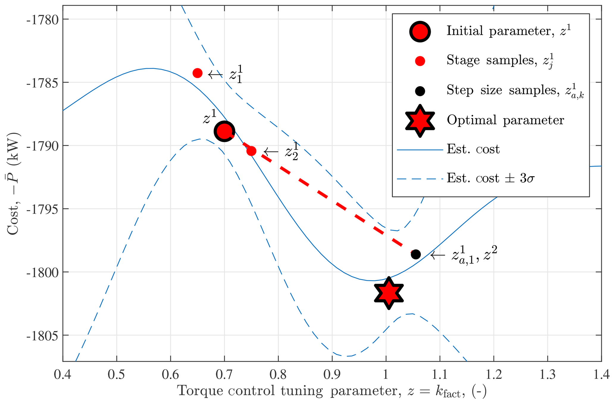
Figure 1 The first iteration of the one-dimensional parameter tuning for the optimal torque control gain. Starting with the initial parameter z¹, random samples ${\mathit{z}}_{\mathrm{1}}^{\mathrm{1}}$ and ${\mathit{z}}_{\mathrm{2}}^{\mathrm{1}}$ are generated to estimate the gradient. The test sample ${\mathit{z}}_{a,\mathrm{1}}^{\mathrm{1}}$ is evaluated in the gradient direction until the cost decreases and the next stage parameter z² is determined. The estimated cost and uncertainty shown are determined after r=1 stage (four parameters and 12 total simulations) and found using Eqs. (13) and (19), respectively, where $\mathit{\sigma }\left(\mathit{z}\right)=\sqrt{\mathrm{MSE}\left[\widehat{C}\right(\mathit{z}\left)\right]}$.

The optimal value of k_fact is expected to be between 0.3 and 1.7, so these values are set as hard bounds. A search range of μ=0.05 is set to adequately search the space and estimate meaningful gradients. For tuning controllers of turbines with different power ratings, the base step size is scaled with the inverse of the initial simulation's average power $\stackrel{\mathrm{‾}}{P}\left({\mathit{z}}^{\mathrm{1}}\right)$. Larger power values result in larger gradients; since the scale of the parameter is constant for all rotors (it should ideally be 1), the step size should be reduced to maintain the same rate of descent. Note that a positive step size is required, even though the cost is negative, and a maximum of three step size sample simulations are performed (k_max=3). A summary of the parameters used in the torque control parameter optimization is shown in Table 1, and an illustration of the first iteration is shown in Fig. 1.

Table 1 Design choices for 1-D parameter search to optimize the torque gain in below-rated control.

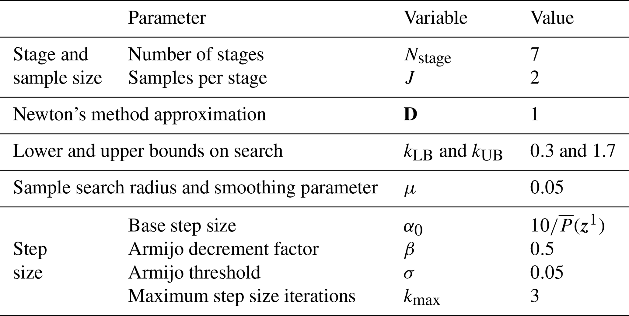
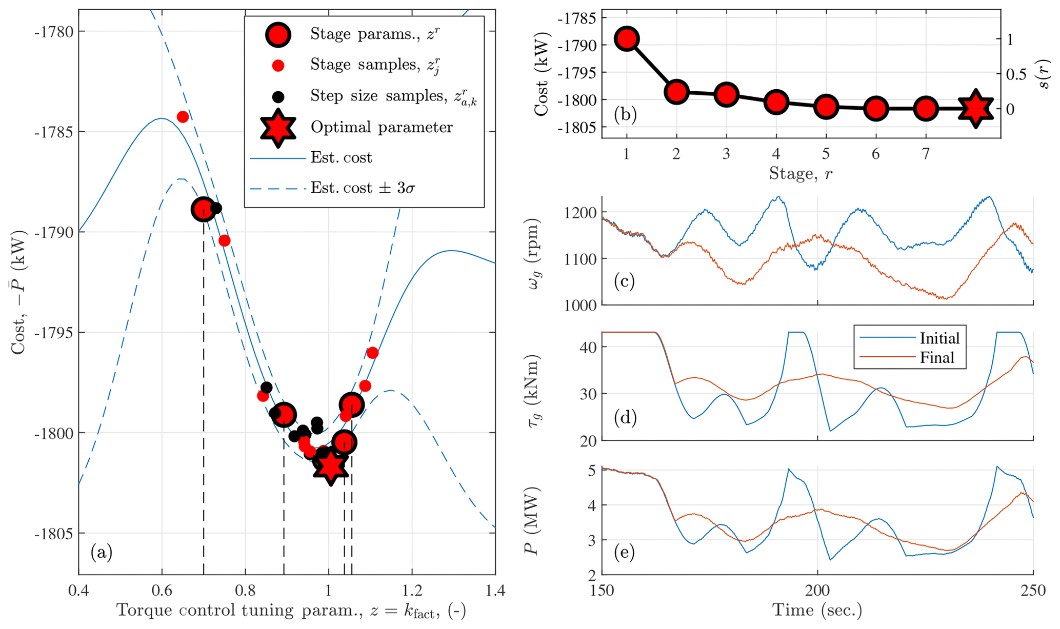
Figure 2 One-dimensional parameter tuning for the optimal torque control gain of the 5 MW reference turbine in Class A turbulence using the negative mean generator power ($-\stackrel{\mathrm{‾}}{P}$) as the cost function. In below-rated control, the generator speed (ω_g) is controlled using the generator torque (τ_g). The estimated cost and uncertainty are found using Eqs. (13) and (19), respectively, where $\mathit{\sigma }\left(\mathit{z}\right)=\sqrt{\mathrm{MSE}\left[\widehat{C}\right(\mathit{z}\left)\right]}$. The settling function s(r) is defined in Eq. (21) and the cost estimate is determined using all of the simulation results (27 unique parameters in 81 total simulations).

The parameter optimization was performed on the NREL-5MW reference turbine with the standard lookup-table-based torque controller in Jonkman et al. (2009). The algorithm finds close to the optimal k_fact in five stages and realizes diminishing returns thereafter (Fig. 2b). The full procedure, with seven stages, performs 81 simulations in total, which includes step size samples and the initial guess. If only a single simulation at 8 m s⁻¹ is used and the controller is exclusively in region II, we find a lower optimal k_fact than is shown in Fig. 2a (Zalkind et al., 2020). By including other wind speeds and the transition region, as shown in Fig. 2c, d, and e, the optimal k_fact is nearly 1. The use of turbulent simulations contributes noise to the signal that determines the cost function, which is apparent by the nonsmooth behavior of the cost samples with respect to the gain factor parameter in Fig. 2a. However, the algorithm appears to be robust to these uncertainties.

3.2 Pitch control for generator speed regulation

In this section, we optimize the parameters of an above-rated blade pitch controller for load reduction and generator speed regulation. Each time a new rotor is designed, the pitch controller should be tuned so that the structural loads can be computed to design the various hardware components of the wind turbine. As will be seen, the pitch controller affects the loads that drive turbine design. The procedure for tuning the gain-scheduled proportional–integral (PI) controller is detailed in Appendix A. First, steady-state simulations at above-rated wind speeds are used to determine the turbine operating points and aerodynamic parameters at various pitch angles, which parameterizes the gain scheduling. The final, and most involved, step is to tune the natural frequency (ω_reg) and damping ratio (ζ_reg) of the “regulator mode,” which represents the generator speed response to a disturbance (wind) input. The following optimization procedure aims to find an optimal set of parameters (ω_reg,ζ_reg) so that structural loads are minimized and adequate generator regulation is maintained.

In general, changing the bandwidth of the pitch controller via ω_reg alters the structural loading of various components, which we denote generically with M in the following. In this section, we use M to denote tower fatigue or peak blade loading, though any load could be used that results in a feasible optimization problem; the control and hardware designers must determine what loads are important to the overall turbine design. However, controllers with lower natural frequencies allow greater generator speed transients, which is acceptable up to some maximum constraint. If the generator speed exceeds some threshold ω_g,hard, most turbines enter into a shutdown procedure to avoid further damage, which reduces the availability of the turbine and the net annual energy production; this must be avoided.

First, we reformulate the constrained optimization

$$\begin{array}{}\text{(27)}& {\displaystyle }\underset{\mathit{z}=({\mathit{\omega }}_{\mathrm{reg}},{\mathit{\zeta }}_{\mathrm{reg}})}{min}M\left(\mathit{z}\right)\text{(28)}& {\displaystyle }\mathrm{subject}\mathrm{to}{\mathit{\omega }}_{\mathrm{g}}\le {\mathit{\omega }}_{\mathrm{g},\mathrm{hard}}\end{array}$$

as an unconstrained problem to use the algorithm described in Sect. 2. The cost function is augmented so that the optimization problem has the form in Eq. (1), namely

$$\begin{array}{}\text{(29)}& \mathcal{C}\left(\mathit{z}\right)=M\left(\mathit{z}\right)+B\left(\mathit{z}\right),\end{array}$$

where B(z) is a boundary function that penalizes samples that have a maximum generator speed that exceeds some “soft” generator speed constraint ω_g,soft,

$$\begin{array}{}\text{(30)}& B\left(\mathit{z}\right)=\left\{\begin{array}{ll}\mathrm{0}& \mathrm{if}{\mathit{\omega }}_{\mathrm{g},\max }\left(\mathit{z}\right)<{\mathit{\omega }}_{\mathrm{g},\mathrm{soft}}\\ k_B\left({\mathit{\omega }}_{\mathrm{g},\max }\right(\mathit{z})-{\mathit{\omega }}_{\mathrm{g},\mathrm{soft}}{)}^{\mathrm{2}}& \mathrm{otherwise}.\end{array}\right.\end{array}$$

A quadratic boundary function is used so that the cost is differentiable, even when a nonfeasible solution is sampled. The factor k_B is chosen to provide a sufficient penalty on high generator speeds but not so high that exceedingly large gradients are determined from the gradient estimation in Eq. (3), which can be problematic for the algorithm.

$$\begin{array}{}\text{(31)}& k_B={\displaystyle \frac{c_{\max }}{({\mathit{\omega }}_{\mathrm{g},\mathrm{hard}}-{\mathit{\omega }}_{\mathrm{g},\mathrm{soft}}{)}^{\mathrm{2}}}}\end{array}$$

ensures that the barrier function B(z)=c_max when the maximum generator speed equals the hard generator speed constraint ω_g,hard.

To adapt the cost function to different rotors and load measures,

$$\begin{array}{}\text{(32)}& c_{\max }={\displaystyle \frac{\mathrm{1}}{\mathrm{12}}}M\left({\mathit{z}}^{\mathrm{1}}\right),\end{array}$$

where M(z¹) is the load measure of the initial stage sample and the factor $\frac{\mathrm{1}}{\mathrm{12}}$ is based on experience gained using the algorithm with simulation results. A smaller factor does not penalize maximum generator speeds enough, leading to possibly infeasible solutions that violate Eq. (28). Factors greater than $\frac{\mathrm{1}}{\mathrm{12}}$ were found to create large gradients that lead the iterates away from the constraint boundary; typically, the optimal solution is found close to that boundary.

Table 2 Parameters used for the 2-D speed regulator control tuning procedure for all rotors tested. The effects of the number of stages N_stage and samples per stage J on the algorithm's performance are investigated in Section 3.2.2.

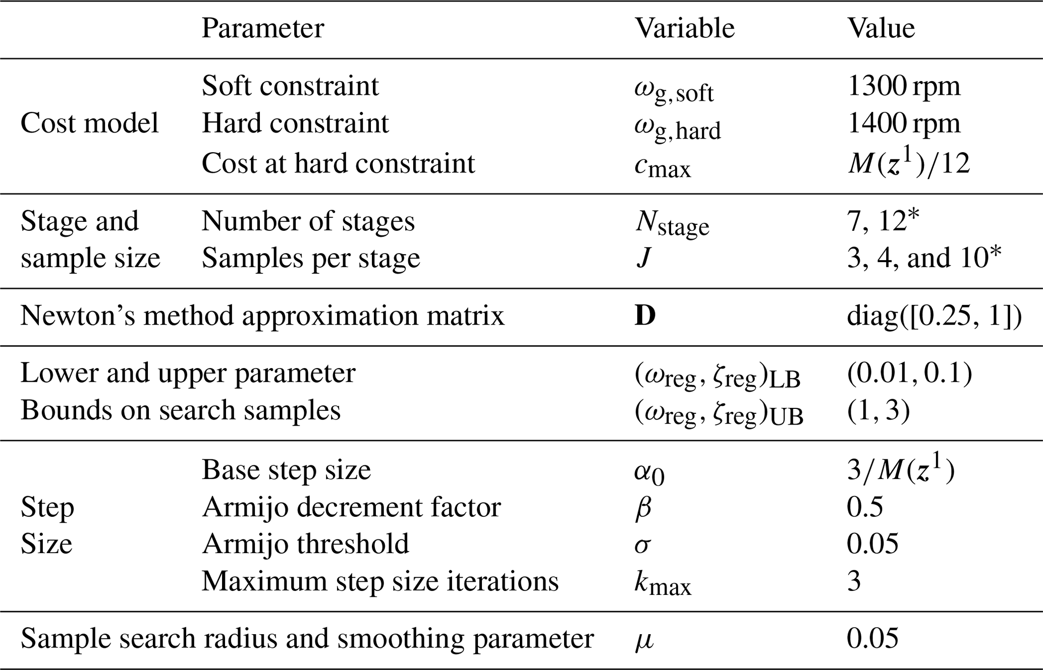
^* In Sect. 3.2.2, we compare the performance of using different numbers of stages N_stage and samples per stage J.

In most cases, the initial parameter set z¹ is chosen to be near values that were tuned manually but offset (usually with a higher natural frequency) to allow the algorithm to converge properly. If the parameters were not previously tuned, the values suggested in the NREL-5MW reference manual (Jonkman et al., 2009) are chosen as the initial parameter set. A summary of the parameters used to tune all the rotors in this study is presented in Table 2. The algorithm is tested using different numbers of stages N_stage and samples per stage J in Sect. 3.2.2. The best results were achieved using a quasi-deterministic search direction,

$$\begin{array}{}\text{(33)}& {\mathit{\varphi }}_j^r=[\cos {\mathit{\psi }}_j,\sin {\mathit{\psi }}_j{]}^{\mathrm{T}},\end{array}$$

where

$$\begin{array}{}\text{(34)}& {\mathit{\psi }}_j={\mathit{\psi }}_{\mathrm{0}}+{\displaystyle \frac{\mathrm{2}\mathit{\pi }j}{\mathrm{3}}},\end{array}$$

is used to evenly space the samples in the two dimensions (ω_reg,ζ_reg), and ψ₀ is randomly generated according to ${\mathit{\psi }}_{\mathrm{0}}\sim U(\mathrm{0},\mathrm{2}\mathit{\pi })$, resulting in the generated samples ${\mathit{z}}_j^{\mathrm{1}}$ in Fig. 3.

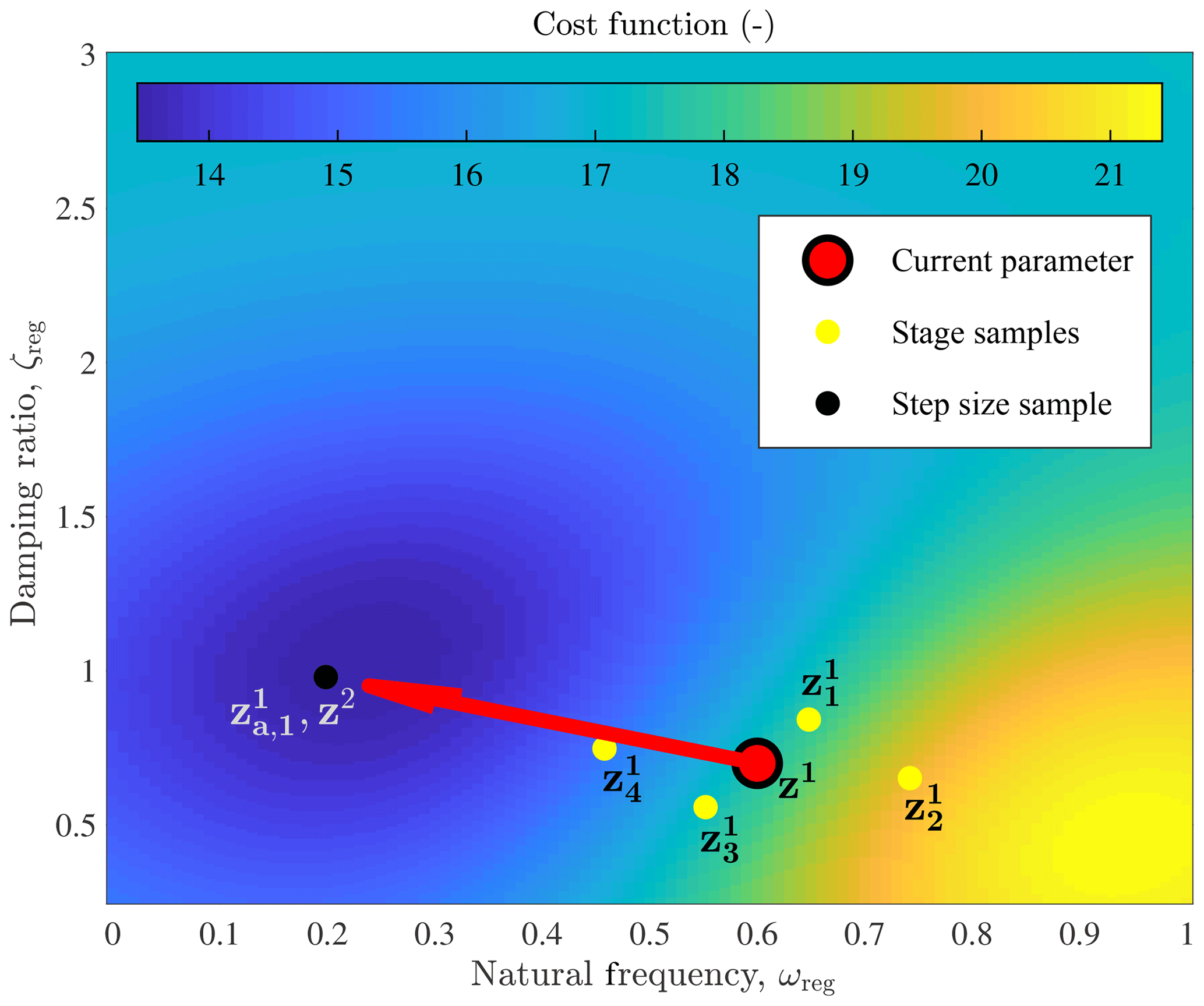
Figure 3 First iteration of the zeroth-order parameter optimization algorithm for the two-dimensional pitch control tuning. Random samples ${\mathit{z}}_j^{\mathrm{1}},j=\mathrm{1}\mathrm{\dots }\mathrm{4}$, are generated near the initial guess z¹ to estimate the gradient. Note that μ=0.15 in this figure for clarity. The sample ${\mathit{z}}_{a,k}^{\mathrm{1}},k=\mathrm{1}$, is tested along the descent direction until a sample with a decreasing cost function is found, which becomes the next guess z² for the pitch control parameter. The cost estimate (background image) is determined after the first stage (r=1, six total simulations).

The cost function is more sensitive to changes in ω_reg than it is to changes in ζ_reg, so $\mathbf{D}=\mathrm{diag}\left(\right[\mathrm{0.25},\mathrm{1}\left]\right)$ was chosen to relatively increase the search direction in the ζ_reg dimension. Hard bounds on (ω_reg,ζ_reg) are chosen to avoid unstable parameter sets. The base step size α₀ scales with the inverse of the initial load M(z¹) so that the algorithm works for turbine models of different sizes, with initial loads specified in Table 3.

Table 3 Summary of test cases and results from a single zeroth-order parameter tuning for speed regulation control using the parameters in Table 2 with N_stage=7 and J=3.

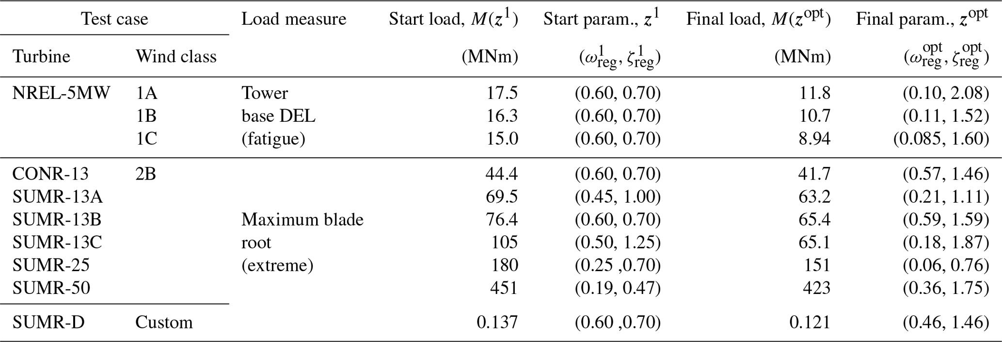
The algorithm was tested on a range of rotor models with different wind classes and load measures. First, the pitch control parameters of the NREL-5MW reference model are optimized, starting from the parameters specified by the NREL-5MW reference manual (Jonkman et al., 2009), and using the tower base moment (fore–aft) damage equivalent load (DEL) as the load measure. For three different wind classes (1A, 1B, and 1C), with different turbulence levels (A – highest and C – lowest), the parameters were optimized, and an example is shown in Fig. 4. In Fig. 5, the estimated cost (a), load (c), and maximum generator speed (e) across the parameter space is shown, along with the estimated uncertainty in (b), (d), and (f). The lowest turbulence level (Class 1C) has the lowest optimal natural frequency ω_reg, since the reduced turbulence results in lower generator speed transients. In each case of the NREL-5MW reference model, the optimized parameters have a lower natural frequency and higher damping ratio than the original setting.

Figure 4 Results of using the zeroth-order optimization for tuning the pitch control regulator mode (natural frequency ω_reg and damping ratio ζ_reg) of the 5 MW reference turbine in Class B turbulence using the tower base fore–aft (m_ty) DEL as the load measure, which is indirectly controlled via θ_c, the collective blade pitch control; θ_c is primarily responsible for regulating the generator speed ω_g. The settling function s(r) is defined in Eq. (21). The cost estimate (background image in Fig. a) is determined after $r=N_{\mathrm{stage}}=\mathrm{7}$ stages (a total of 42 parameter pairs and simulations).

The optimization procedure was also performed for each rotor design in the Segmented Ultralight Morphing Rotor (SUMR) project (Loth et al., 2016); for these rotors, the design driving load case for blade design was the maximum blade root bending moment. In practice, the combined edgewise and flapwise load is used for design, but since the edgewise load is deterministic, we used the maximum flapwise load as the load measure for optimization, which is a good indicator of maximum combined loads. The SUMR rotor radii range in size from 22 to 240 m (Appendix Table B1), and the same optimization parameters (Table 2) were used for each optimization procedure, albeit with different initial conditions and loads, which adapt the cost function and step size accordingly. The optimization procedure generally settles on a lower natural frequency and higher damping ratio than the initial guesses (Table 3), which has the effect of producing the lowest control bandwidth (for reducing loads) but only to the point so that the generator speed constraint is not exceeded.

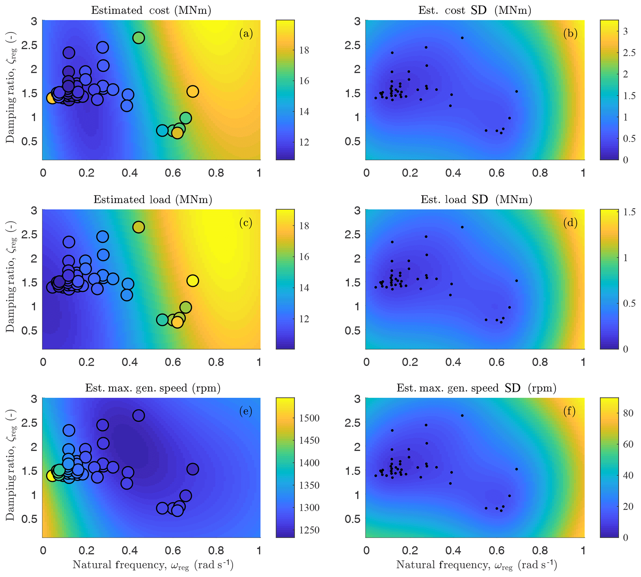
Figure 5 Cost (a), load (c), and generator speed (e) estimated values and standard deviations (SD; b, d, and f) using the kriging visualization described in Sect. 2.6. The sample values are shown in (a), (c), and (e), and their locations are depicted in (b), (d), and (f).

3.2.1 Discussion of low natural frequency, high damping ratio regulator mode

For most of the rotors in this section, the baseline rotor speed proportional–integral (PI) control parameters are optimized to have a regulator mode with a lower natural frequency and higher damping ratio than the initial guess (Table 3). To understand why this is the case, we must consider the cost function of the optimization. In this tuning procedure, our goal is to minimize structural loading with a constraint on the maximum generator speed. From Fig. 4c and d, we see that the collective blade pitch angle θ_c has a large effect on the thrust-based structural loading; this includes tower fatigue and blade peak loads. Figure 4 shows that, in most cases, pitch and loads mirror each other: when pitch increases, loads decrease, and vice versa. A good example occurs between 230 and 250 s in the time series of Fig. 4. The direct effect of the blade pitch signal on the load signal is the primary reason for the optimal PI gains (or regulator mode parameters) found in this section.

PI gains derived from a regulator mode with a low natural frequency result in less pitch actuation and thus less change in the load. Higher natural frequencies result in faster and more frequent pitch control variations, which translate to the structural load signals and increase fatigue loading. A controller with a high natural frequency can also be problematic when the wind speed decreases. Because the underlying controller is trying to regulate the generator speed, the pitch will decrease during a wind lull to maintain the generator speed at its rated value, which can also lead to large peak loads, especially when an increase in wind speed follows.

High damping ratios are also found to be optimal when using the described cost function. A generator speed response and pitch control response with a high damping ratio lacks any overshoot and secondary transients when the system is subjected to a disturbance (wind). Secondary transients and overshoot in the pitch command result in load transients. The original NREL-5MW controller (where ω_reg=0.6 rad s⁻¹, ζ_reg=0.7) has regulator mode poles at $-\mathrm{0.35}\pm j\mathrm{0.45}$, indicative of a fast response with overshoot and transients in the pitch and generator speed signals. The optimized controller in Class 1A turbulence (with ω_reg=0.10 rad s⁻¹, ζ_reg=2.08) has two real poles at −0.40 and −0.025, which results in a fast initial pitch response and a slower secondary response.

When comparing the PI gains of the original versus optimized controller, we see that the proportional gains are of similar magnitudes, but the integral gain is much less in the optimized set of gains. The original NREL-5MW gains are $k_{P,\mathrm{0}}=\mathrm{2.3}\times {\mathrm{10}}^{-\mathrm{2}}$ s and $k_{I,\mathrm{0}}=\mathrm{1.0}\times {\mathrm{10}}^{-\mathrm{2}}$, whereas the optimized gains (in Class 1A turbulence) are $k_{P,\mathrm{0}}=\mathrm{1.1}\times {\mathrm{10}}^{-\mathrm{2}}$ s and $k_{I,\mathrm{0}}=\mathrm{0.023}\times {\mathrm{10}}^{-\mathrm{2}}$. These optimized gains reflect the cost function and control goal and environmental setting; we assume that special and fault cases would be handled by a supervisory controller. The optimized proportional gain is still large enough to mitigate generator speed transients, ensuring that the generator speed does not exceed the maximum threshold, while the integral gain is reduced because it causes transients in the blade pitch and structural loads. Since our primary goal is not to regulate the generator speed to some fixed set point but instead constrain its maximum value, integral control is less important. If the cost function included a term related to regulating the generator speed to its rated set point, using, e.g., mean squared error compared to the rated generator speed, the optimal integral gains might be larger. However, we believe that a controller that constrains extreme events and maximizes power capture better reflects the overall wind turbine design goals. Typical pitch controllers are designed to regulate the generator speed to some fixed rotor speed with a high enough bandwidth so that the maximum generator speed constraint is not violated. Instead of focusing on a quantity that measures how well the generator speed is regulated, we focus on whether or not the maximum generator speed constraint is violated. An initial investigation (Zalkind and Pao, 2019) of the loads on the other turbine components shows a reduction in blade and low-speed shaft fatigue and pitch actuation, but a more in-depth load investigation is left for future work.

3.2.2 Results: comparison with grid searching

To quantify the performance of the zeroth-order optimization (ZOO) for this pitch control application, we compare it, in terms of the number of simulations and optimal cost, with a grid search optimization for tuning the pitch controller of the NREL-5MW reference turbine in Class 1A turbulence. The same area spanned by the hard bounds of the zeroth-order method (Table 2) is sampled by a N_grid×N_grid grid, with $N_{\mathrm{grid}}=\mathrm{6},\mathrm{8},\mathrm{and}\mathrm{10}$. The cost, defined by Eqs. (29)–(32) and sampled using the N_grid=10 grid search, is shown in the background of Fig. 6a–e. The parameter z with the minimum cost over all simulations in the search is the optimal parameter z^opt. In practice, we would refine the search area and resample based on experience. However, different models may change the resampled area and would add a manual step that we can avoid when using the zeroth-order optimization procedure.

Figure 6 Panels (a)–(d) show the result of performing the zeroth-order optimization (ZOO) for the baseline rotor speed controller using N_stage=7 and 12 stages and $J=\mathrm{3},\mathrm{4},\mathrm{and}\mathrm{10}$ samples per stage, using four different initial conditions (z¹). The background image of panels (a)–(e) is of the cost function, sampled using a grid search with a 10×10 level of precision using the hard bounds in Table 2 and normalized to the cost when z¹=z^sug. Panel (e) shows the optimal solutions of three different grid search resolutions. Panel (f) compares the optimal costs, normalized to the initial cost when z¹=z^sug, compared with the number of simulations used to find the result.

The ZOO procedure outlined in Sect. 2 is performed three times for each of the following cases. Each procedure uses randomly generated samples that should result in different optimal parameters for each instance. We use four different initial conditions, distributed so that one is in each of the four quadrants spanning the bounded parameter space. The starting location in each quadrant was generated randomly, except for the bottom, right quadrant in Fig. 6d, which is the suggested parameter set, ${\mathit{z}}^{\mathrm{sug}}=({\mathit{\omega }}_{\mathrm{reg}},{\mathit{\zeta }}_{\mathrm{reg}})=(\mathrm{0.6},\mathrm{0.7})$, defined in the NREL-5MW reference manual (Jonkman et al., 2009). The ZOO was performed with N_stage=7 stages using $J=\mathrm{3},\mathrm{4},\mathrm{and}\mathrm{10}$ samples per stage and also with N_stage=12 using J=3 samples per stage. Theoretical results suggest that better gradient estimates (from a larger number of samples per stage J) result in convergence within a ball with a smaller radius centered around an optimal solution (Hajinezhad et al., 2017). The optimal parameter set z^opt found in each instance of the ZOO is shown in Fig. 6a–d. We compare the cost of the ZOO method with the grid search optimization in terms of the defined cost function in Eqs. (29)–(32) (Fig. 6f). The results are normalized to the cost function found using the suggested parameter set z^sug.

Compared to z^sug, all of the methods result in a 20 % to 26 % reduction in the cost function, with about a 1 % standard deviation in the results. For fewer than 80 simulations in this application, ZOO performs better than the grid search benchmark in almost every case. The optimal cost decreases with increasing J and total number of simulations on average, but not necessarily always. However, in terms of efficiency on a per-simulation basis, J=3 (blue in Fig. 6) achieves similar results to those found using J=10 (yellow in Fig. 6). Additional stages (N_stage=12) with J=3 (purple in Fig. 6) decrease the cost function further; the optimal cost of this case is the best we tested in terms of the number of simulations and cost reduction. By a small margin (1 %–2 %), using the initial parameter z¹=z^sug in the bottom, right quadrant in Fig. 6d performed better than the other z¹ locations shown in Fig. 6a–c. In Fig. 6a–d, we see that if we use a z¹ that is closer to the area where z^opt is found, there is less variation in z^opt; there is also less variation in the minimum cost 𝒞(z^opt).

We should note that the comparison presented in this section applies only to this pitch control tuning application. To compare the efficacy of the zeroth-order optimization with a grid search more generally would require comparing functions of different complexities and dimensions, which is outside the scope of this article and we leave for future work.

3.3 Minimum pitch setting for peak load reduction

In this final example, a series of one-dimensional parameter optimizations will be used to tune the minimum pitch setting of the above-rated pitch controller described in Appendix A and shown in Fig. A1. Increasing the minimum pitch setting can reduce the peak blade and tower loads. However, it also slightly reduces power capture. To represent this trade-off, the cost function

$$\begin{array}{}\text{(35)}& C\left(\mathit{z}\right)=\mathit{\kappa }{\displaystyle \frac{M\left(\mathit{z}\right)}{M\left({\mathit{z}}^{\mathrm{0}}\right)}}+(\mathrm{1}-\mathit{\kappa }){\displaystyle \frac{\stackrel{\mathrm{‾}}{P}\left({\mathit{z}}^{\mathrm{0}}\right)}{\stackrel{\mathrm{‾}}{P}\left(\mathit{z}\right)}}\end{array}$$

will be minimized, quantifying the relative importance κ between reducing peak loads and reducing power capture, where z=θ_min(u) is the minimum pitch setting at wind speed u, M is the maximum blade flapwise load (over all blades), and $\stackrel{\mathrm{‾}}{P}$ is the mean generator power of a turbulent simulation with mean wind speed u. A value of κ=0.01 is used, which represents a 10 % reduction in peak load being roughly equal to a 0.1 % decrease in power capture; this parameter can be tuned by the control designer based on the goals of the design; however, the feasibility of the optimization problem should be verified. In future work, a family of optimal minimum pitch control laws, using different values for κ, could be generated but would require more global wind turbine design information to determine the design choice.

During the load analysis of a control design, a number (N_seeds) of randomly generated turbulent seeds are used to simulate the turbine across wind speeds to identify peak loads on the various components. Often, peak loads on the blade and tower occur in situations where there is first a lull in the wind speed, which causes the pitch angle to decrease, followed by an increase in wind speed. If the pitch controller does not react in time, the combination of high wind speeds and low pitch angles causes a large thrust on the rotor. However, if the minimum allowable pitch is increased, the peak loads resulting from wind speed lulls can be reduced. An example is shown in Fig. 7c and d at 275 s. While these events are fairly common in simulation, not all produce equal peak loads; the minimum pitch setting is optimized for the worst-case simulation.

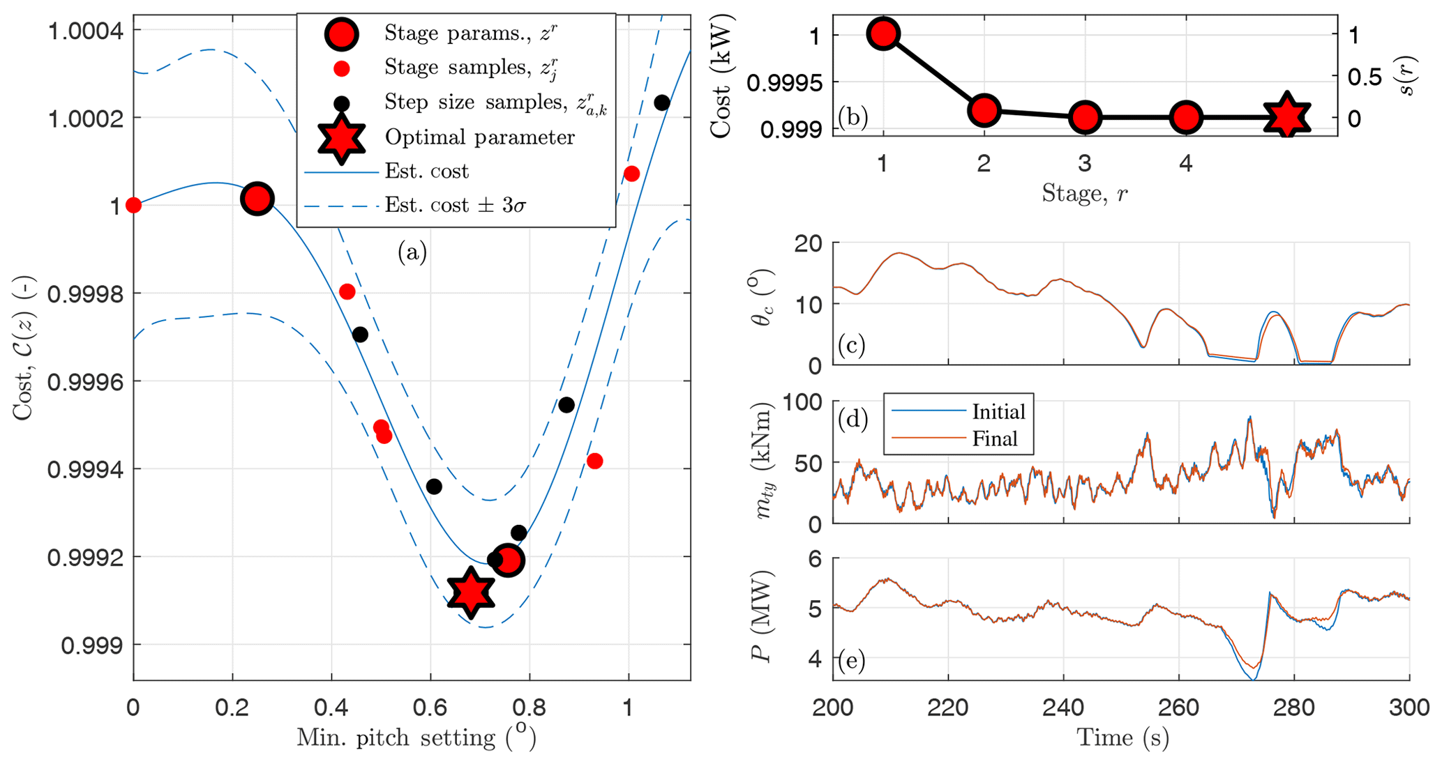
Figure 7 A zeroth-order optimization for the minimum pitch setting at 14 ms⁻¹ for the NREL-5MW reference turbine. The cost 𝒞(z) in Eq. (35) is a function of the peak tower load m_ty and mean of the generator power P in the simulation, where θ_c is the collective pitch angle. The settling function s(r) is defined in Eq. (21) and the cost estimate is determined using all of the simulation results (15 unique pitch settings and simulations).

A wind speed estimate, which can be found using, e.g., one of the methods in Soltani et al. (2013), is used to determine the minimum pitch setting of the above-rated pitch controller. A smooth lookup table is generated using a cubic spline interpolation and a table of three minimum blade pitch settings with breakpoints at above-rated wind speeds, in addition to a breakpoint in below-rated wind speeds and one above the cut-out wind speed. The minimum pitch setting is nondecreasing with respect to wind speed. An example is shown in Fig. 8. The minimum pitch at each above-rated breakpoint will be optimized using the zeroth-order optimization procedure previously described.

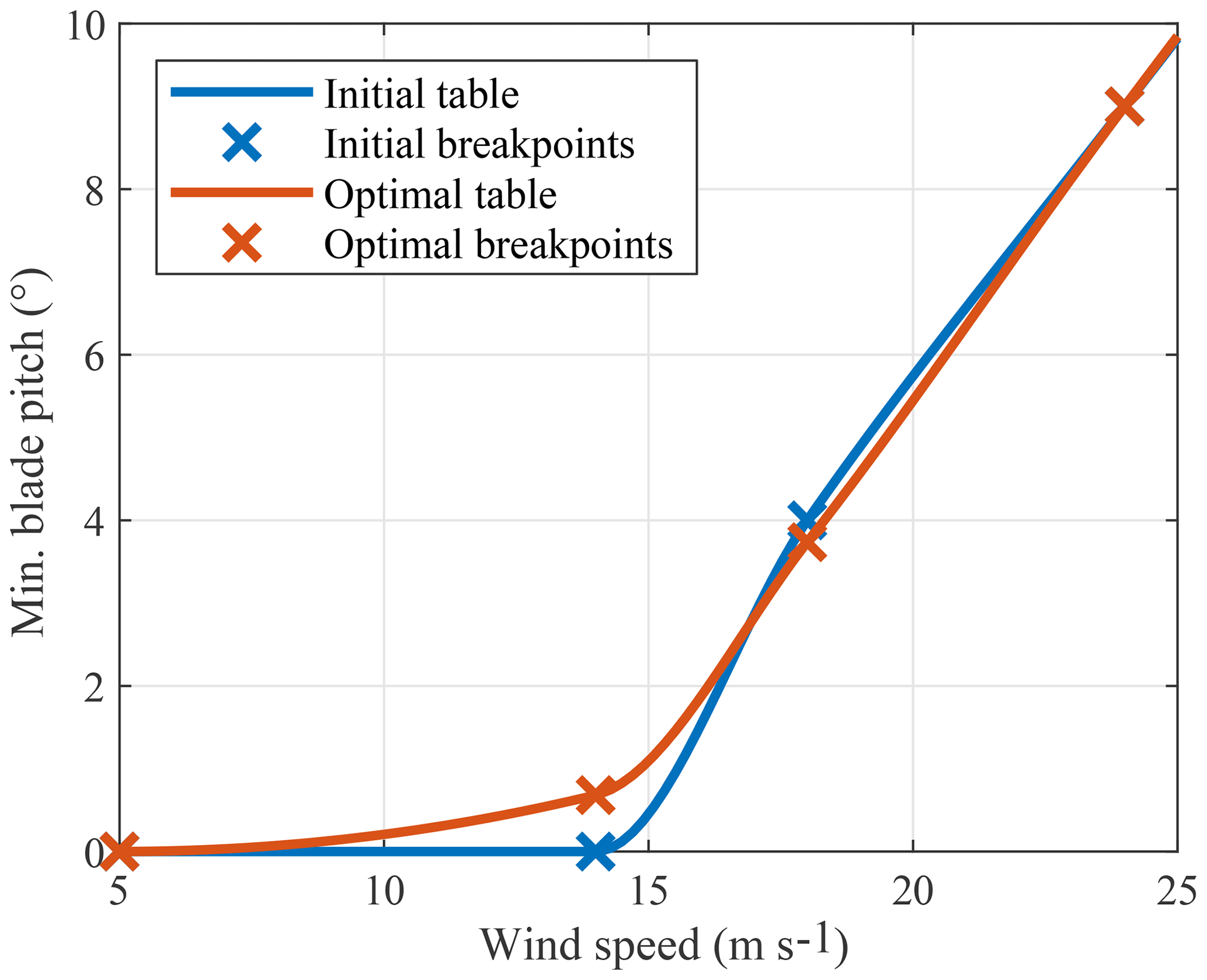
Figure 8 Minimum pitch setting as a function of wind speed. Each active breakpoint is tuned in a series of one-dimensional parameter optimizations. There is an additional high wind speed breakpoint at 50 ms⁻¹.

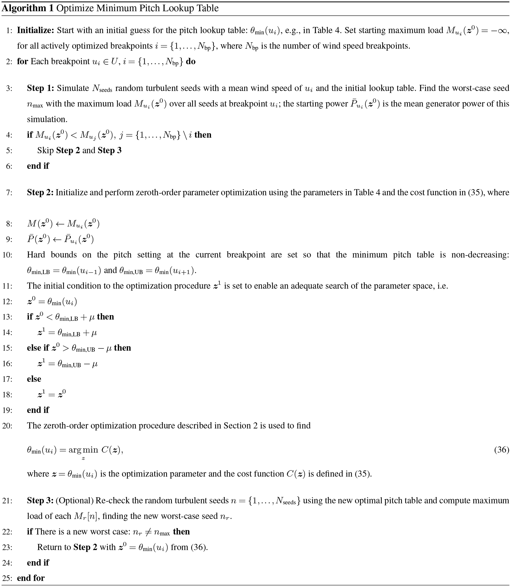
The algorithm (presented in Algorithm 1) is initialized by choosing an initial lookup table for the minimum blade pitch, θ_min(u_i) in Table 4. In Step 1, N_seeds random seeds are simulated to find the worst-case seed n_max with the maximum load at that breakpoint $M_{u_i}\left({\mathit{z}}^{\mathrm{0}}\right)$. The optimization procedure in Step 2 is only performed if the current breakpoint has a problematic peak load: one that is greater than loads seen at the other mean wind speeds (line 4 of Algorithm 1). The starting loads are initialized to $M_{u_i}\left({\mathit{z}}^{\mathrm{0}}\right)=-\mathrm{\infty }$ so that at least the first active breakpoint is optimized. At the low wind speed breakpoint u₀=5 ms⁻¹, the minimum pitch angle is set to the aerodynamically optimal angle θ_fine; and at the high wind speed breakpoint $u_{N_{\mathrm{bp}}+\mathrm{1}}=\mathrm{50}$ ms⁻¹, the optimal minimum pitch angle is set to the feather pitch angle. Neither u₀ nor $u_{N_{\mathrm{bp}}+\mathrm{1}}$ is an actively optimized breakpoint; they are, however, used as lower and upper bounds for the first u₁ and last $u_{N_{\mathrm{bp}}}$ active breakpoints.

In Step 2, the initial guess that is used by the optimization procedure (z¹) is offset from the lower and upper bounds by the sample search area μ (lines 11–19 of Algorithm 1). Step 3 is optionally performed to recheck the other random turbulent seeds using the new, optimized minimum pitch lookup table. In some cases, a different random seed will have a peak load that exceeds that of the wind input that was originally optimized; if this is the case, Step 2 is repeated up to three times, using the previously optimized pitch angle as a lower bound.

Table 4 Parameters used to optimize the minimum pitch lookup table.

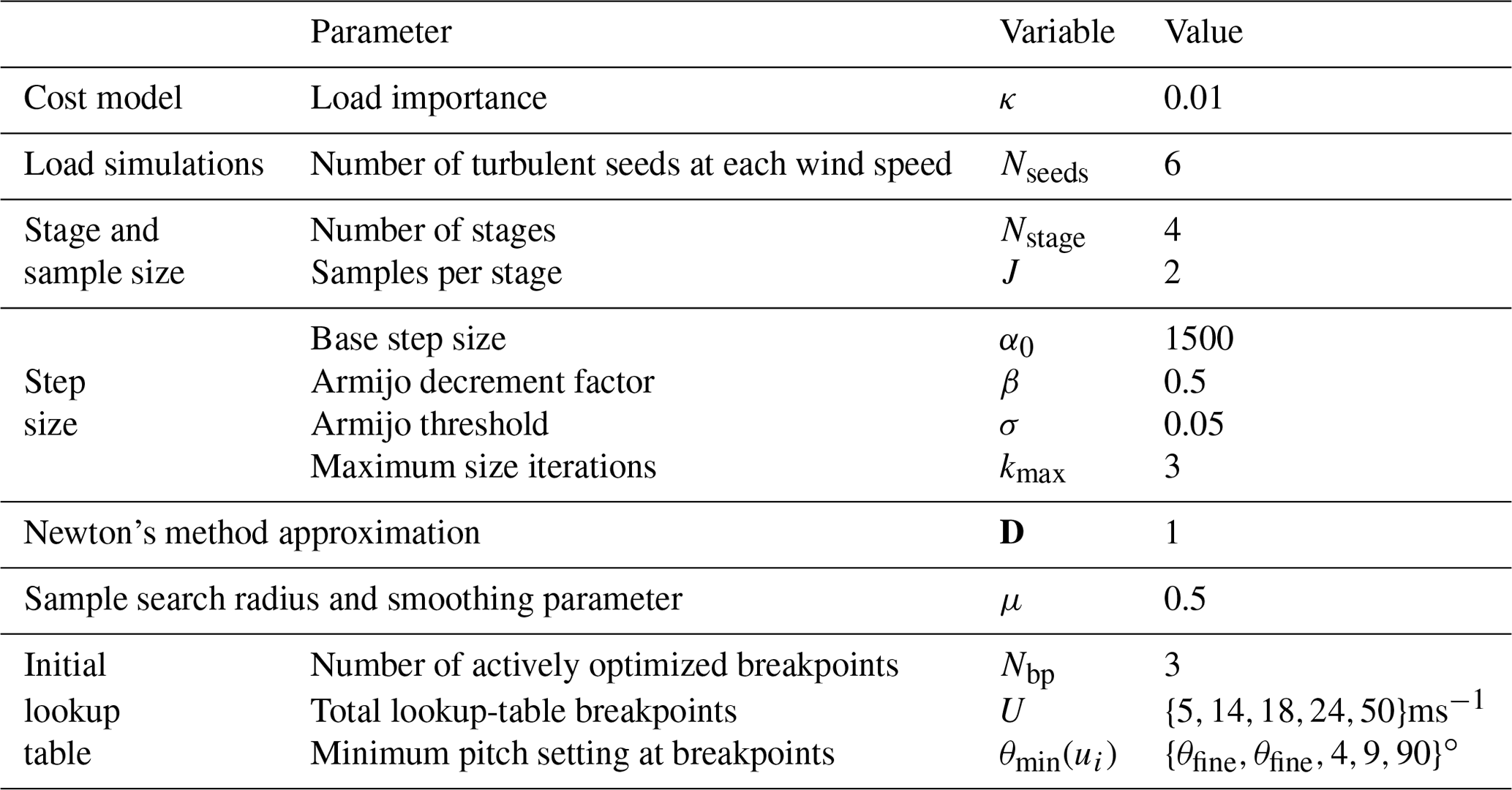
Algorithm 1 is used to optimize the minimum pitch table in Fig. 8 using the parameters in Table 4 and the SUMR-13A wind turbine model. Six random turbulent seeds are initially simulated and only the 14 and 18 ms⁻¹ breakpoints require optimization (the peak loads of the 24 ms⁻¹ simulations are all less than the 14 and 18 ms⁻¹ loads). N_stage=4 stages with J=2 samples per stage are used to optimize the 14 ms⁻¹ breakpoint; the results of the procedure are depicted in Fig. 7.

3.4 Coupling between control optimizations and systems engineering considerations

Changing the minimum pitch setting of the controller can have an effect on the below-rated power production (optimized in Sect. 3.1) and peak and fatigue loads (optimized in Sect. 3.2). Though this coupling exists, in our experience, the effect on the optimized parameters is small.

In future work, a multiobjective optimization might be more suitable, where all the tuning procedures are simultaneously performed; the zeroth-order method is suitable in this case. A potential challenge would be determining what simulations should be used to efficiently optimize all of the control parameters. Currently, each control tuning procedure requires running different simulations. Additionally, the goal of this work was to automate design choices, rather than having to choose from a set of possible choices that would result from a multiobjective optimization.

However, with additional resources, our goal could shift from efficient optimization of smaller problems to larger optimizations of the overall turbine system. Within a system engineering framework, more information might determine which simulations and loads are sensitive to control parameter changes. In this article, we focused on minimizing the peak blade loads of the SUMR rotors because those were the design driving load of those blades. Other loads could certainly be used, but all loads are not important to the overall design: some components are overdesigned, and others drive design; this information depends on the specific design but could be determined using detailed system engineering tools.

Our goal was to reduce the design cycle times for processes that already occur during control design. Rather than solving all problems at once, we propose solving them in sequence, in the order they are presented: first optimizing the torque and pitch controllers and then tuning the minimum pitch setting for peak loads. Then with the new minimum pitch table, a designer could optionally reoptimize the torque and pitch gains; we have done this and witness little change. Solving smaller problems tends to be more efficient in terms of the number of simulations and more transparent in terms of how control parameters affect different performance measures during specific simulations. We discuss setting up similar optimization problems for future work in Sect. 4.

4 Generalized design procedure

In this section, we present guidelines for performing similar optimization procedures. Experience gained in problem formulation, the usefulness of performing a preliminary offline analysis, and the determination of the parameters of the solver is shared.

4.1 Determine problem and goals

Using the zeroth-order optimization procedure described in this article for determining control parameters through simulation requires effort in setting up the problem and developing software. In order to justify the up-front effort, the task would ideally be one that is repeated for many different rotor models, like the examples in Sect. 3. A task that is repeatedly performed also allows the designer to gain a deeper understanding for how control inputs (gains, parameters) affect simulation outputs of the wind turbine.

It is important to determine how the turbine should be simulated in order to generate the measures that are used for the optimization; they should highlight some problematic or indicative case that the control solution is trying to solve. For example, when optimizing the torque control gain for below-rated operation in Sect. 3.1, a below-rated wind field should be used, and the power should be used as the cost function. The cost function should reflect the goals of wind turbine design (e.g., increasing power capture or decreasing loads), have a basis in the reality of wind turbine operation (e.g., using gains that provide a stable control input), and also have a feasible solution. The optimization procedure presented in this article is only useful if the cost function represents the design goal, is represented well by the simulation information, and is simulated in a realistic environment.

4.2 Perform preliminary analysis

It is often helpful to perform a preliminary offline analysis to fine-tune the cost function and optimization parameters. In an offline analysis, a grid search of the optimization parameter is used to estimate the output space of the simulations (e.g., maximum generator speed and blade loads), using a linear or quadratic estimate of the cost function. To clarify, the results in Sect. 3 are of online optimizations, where actual simulation data are used to compute the cost function and perform the optimization procedure. While one of the goals in developing this optimization procedure is to eliminate the large number of simulations associated with grid searching, a grid search does help fine-tune the parameters of future, similar control tuning procedures that use zeroth-order optimization. If multiple measures are used in the cost function (e.g., in the pitch control tuning of Sect. 3.2), it is important to determine whether the cost function has a minimum within the parameter bounds. Otherwise, the cost function must be further refined. A preliminary offline analysis can be used to more quickly determine the optimization parameters (e.g., step size or smoothing parameter) that converge in the fewest number of simulations to some ground truth determined from the estimated cost function based on the initial grid search.

4.3 Set simulation parameters

As the examples of Sect. 3 illustrate, each optimization procedure requires slightly different parameters. While the parameters presented in Tables 1, 2, and 4 may not necessarily be the best ones, they have been fine-tuned through extensive offline testing and evaluating online tests that use actual simulation data as the measures used in the cost function. The goal of this section is to provide general guidelines and rules of thumb, where possible, for choosing the parameters of the optimization procedure.

4.3.1 Sample search range and Newton's approximation

The smoothing parameter μ should be based on the optimization parameter z. The sample z+ϕμ should result in an adequate change to the cost function so that good gradients can be used for the descent algorithm; note that the magnitude of the direction $\left|\right|\mathit{\varphi }\left|\right|=\mathrm{1}$. From the examples in Sect. 3, a different μ is required because the cost function of each application has a different magnitude and changes at different rates. Too large of a μ can result in samples that violate the hard bounds or gradients that do not represent the local gradient at the stage sample. On the other hand, a μ that is too small can result in noisy gradients, the result of possibly nonsmooth simulation information for samples that are close to each other.

When optimizing over multiple parameters, the D matrix is used to approximate Newton's method for optimization. D increases or decreases the descent direction d_r, where the sensitivity of the cost function to that parameter (dimension) is small or large, respectively. Ideally, the matrix D incorporates second-order information to scale the gradient estimate in each dimension. In a true Newton method, where second-order information is available, $\mathbf{D}={\left[\mathbf{H}\mathcal{C}\left(\mathit{z}\right)\right]}^{-\mathrm{1}}$, where H𝒞(z) is the Hessian of the cost function 𝒞 at the parameter z. To approximate Newton's method, we use $\mathbf{D}=\mathrm{diag}\left(\right[D_{\mathrm{1}},\mathrm{\dots },D_M\left]\right)$, where

$$\begin{array}{}\text{(37)}& D_i\approx {\left({\displaystyle \frac{{\partial }^{\mathrm{2}}\mathcal{C}}{\partial \mathit{z}(i{)}^{\mathrm{2}}}}\right)}^{-\mathrm{1}}\end{array}$$

and z(i) is the ith element of the parameter set z. The elements D_i of D can be determined from offline simulation analysis, where Eq. (37) can be estimated by finding a quadratic regression of the cost space. Alternatively, D_i can be manually tuned, i.e., if the dimension i is not being adequately searched, D_i should be increased.

For example, in the pitch controller tuning (Sect. 3.2), the cost function (shown in Fig. 3) is less sensitive to the damping ratio z(2)=ζ_reg than it is to the natural frequency z(1)=ω_reg, so we use $\mathbf{D}=\mathrm{diag}\left(\right[\mathrm{0.25},\mathrm{1}\left]\right)$. If only the first-order (estimated) information were used and the direction of the maximum gradient were exactly followed, the solution would zigzag in the ω_reg direction and take longer to converge to the optimal solution in both the ω_reg and ζ_reg directions.

4.3.2 Step size

The initial step size α₀ is an important parameter to test offline and also fine-tune when using online simulations to compute the gradient. It was found that for all optimization examples in this article, the product of the initial step size and the norm of the gradient should be on the order of a magnitude of 1, namely

$$\begin{array}{}\text{(38)}& \left|\right|{\displaystyle \frac{\partial \mathcal{C}}{\partial \mathit{z}}}\left|\right|\cdot {\mathit{\alpha }}_{\mathrm{0}}\approx \mathrm{0.5}\mathrm{to}\mathrm{1.5}.\end{array}$$

The parameters used in the Armijo step size rule were the same for all examples. Conservative values were used, which essentially only ensures a nonincreasing cost function without a requirement on the rate of descent of the cost function.

4.3.3 Stages and samples per stage

Enough stages should be evaluated so that the cost function converges to some value; this is typically learned through offline analysis or by trial and error in online tests. For example, when analyzing the pitch control tuning results of Fig. 4, the results suggest that the procedure could be performed with fewer stages, whereas it seems more stages could be used in the minimum pitch control tuning of Fig. 7. In general, it is found that fewer samples per stage (along with more stages) result in the fastest convergence with respect to the total number of simulations.

4.3.4 Parameter bounds and initial guess

Hard constraints on the parameter should reflect the set of feasible parameters for the control task being optimized. However, the bounds should not be so small as to restrict the space and possibly miss nonobvious control solutions. The initial guess provided to the algorithm should also allow for the space to be adequately searched.

4.4 Perform optimization and evaluate visualization

After performing initial, offline analysis and running the zeroth-order optimization algorithm using online simulation data, the whole procedure should be evaluated with the following questions:

1. Does the algorithm converge to a feasible solution?

2. Does the optimized parameter appear to be near the minimum of the visualized cost over the parameter space?

An affirmative answer to both of these questions should provide confidence in the optimized result.

5 Conclusions

In this article, we developed a data-driven approach for optimizing controller parameters using simulation results. By using a zeroth-order optimization algorithm, random samples are generated near an initial guess, which are used to compute the local gradient. A standard gradient descent method ensues, where a step size rule is used to ensure convergence and attempt to decrease in the cost function before the next guess is chosen and the process is repeated. We also use ordinary kriging to visualize the design space and its uncertainty to provide a level of confidence in the optimized result.

The zeroth-order algorithm was applied to three different applications in wind turbine control. To demonstrate the process on a one-dimensional parameter optimization, the torque control gain was tuned to optimize power capture in below-rated operation. The baseline pitch controller parameters were tuned in a two-dimensional optimization problem with the goal of minimizing structural loads and include a constraint on the maximum generator speed. Using an adaptable cost function and step size, the algorithm was able to tune the baseline rotor speed control for rotors ranging from 40 to 400 m in diameter. We compare the results, in terms of accuracy, convergence, and number of function evaluations (simulations) for different optimization parameters and against the standard grid search method. In a series of one-dimensional parameter optimizations, we also determined the settings of a lookup table for the minimum pitch limit of the pitch controller, reflecting the overall blade design process and system-level goals.

Since each optimization procedure depends on the specific control problem, we have provided a set of guidelines based on the experience gained during this study for developing future, similar optimization procedures. The methods presented in this article automate a usually manual process, reduce designer effort, and require fewer simulations compared with grid searching methods. These methods can be used for repeated control tuning processes that are required for continually updating designs that must be evaluated in simulation using a well-functioning controller.

Appendix A: Generalized baseline rotor speed pitch controller

The pitch controller described in Sect. 3.2 and 3.3 is based on the controller presented in the NREL-5MW reference manual (Jonkman et al., 2009); this standard control scheme is widely used as a reference for comparing control schemes and evaluating different aspects of turbine design. As shown in Fig. A1, the controller is a gain-scheduled proportional–integral (PI) controller with constant torque above rated. The PI control architecture allows the generator speed dynamics to be represented as a second-order system. Since the sensitivity of aerodynamic torque to blade pitch changes with the blade pitch, the PI gains are scheduled on the blade pitch. The pitch command is saturated to some minimum setting to control power or reduce blade loads; thus, an antiwindup scheme is necessary.

A1 Regulator mode and PI gains

To derive the PI gains for a generic rotor model, a rigid model of the drivetrain is used:

$$\begin{array}{}\text{(A1)}& {\dot{\mathit{\omega }}}_g={\displaystyle \frac{G}{J_{\mathrm{tot}}}}({\mathit{\tau }}_{\mathrm{a}}-G{\mathit{\tau }}_{\mathrm{g}}),\end{array}$$

where ω_g is the generator speed; J_tot is the total drivetrain inertia; including the rotor and generator components; G is the gearbox ratio between the low-speed rotor shaft and the high-speed generator shaft; τ_a is the aerodynamic rotor torque caused by the wind and controlled via blade pitch; and τ_g is the generator torque, which is a control input. The rotor torque is nonlinearly dependent on the blade pitch θ. The linearization with respect to a perturbation in blade pitch δθ is

$$\begin{array}{}\text{(A2)}& \mathit{\delta }{\dot{\mathit{\omega }}}_g={\displaystyle \frac{G}{J_{\mathrm{tot}}}}{\displaystyle \frac{\partial {\mathit{\tau }}_{\mathrm{a}}}{\partial \mathit{\theta }}}\mathit{\delta }\mathit{\theta },\end{array}$$

where the differential torque δτ_g=0 because the torque is constant in above-rated operation. The sensitivity of the aerodynamic torque to rotor speed $\left(\frac{\partial {\mathit{\tau }}_{\mathrm{a}}}{\partial \mathit{\omega }}\right)$ is omitted since it has a much smaller magnitude than $\frac{\partial {\mathit{\tau }}_{\mathrm{a}}}{\partial \mathit{\theta }}$. In terms of power P,

$$\begin{array}{}\text{(A3)}& {\mathit{\tau }}_{\mathrm{a}}={\displaystyle \frac{P\left(\mathit{\theta }\right)G}{{\mathit{\omega }}_{\mathrm{g}}}}\Rightarrow {\displaystyle \frac{\partial {\mathit{\tau }}_{\mathrm{a}}}{\partial \mathit{\theta }}}{|}_{{\mathit{\omega }}_{\mathrm{g}}={\mathit{\omega }}_{\mathrm{rat}}}={\displaystyle \frac{G}{{\mathit{\omega }}_{\mathrm{rat}}}}{\displaystyle \frac{\partial P}{\partial \mathit{\theta }}},\end{array}$$

where ω_rat is the rated generator speed, which is a constant operating point since it is the desired set point of the controller. The proportional–integral control is

$$\begin{array}{}\text{(A4)}& \mathit{\delta }\mathit{\theta }=k_P\mathit{\delta }{\mathit{\omega }}_{\mathrm{g}}+k_I\int \mathit{\delta }{\mathit{\omega }}_{\mathrm{g}}\mathrm{d}t,\end{array}$$

where k_P and k_I are the proportional and integral control gains, respectively, and δω_g represents a generator speed perturbation.

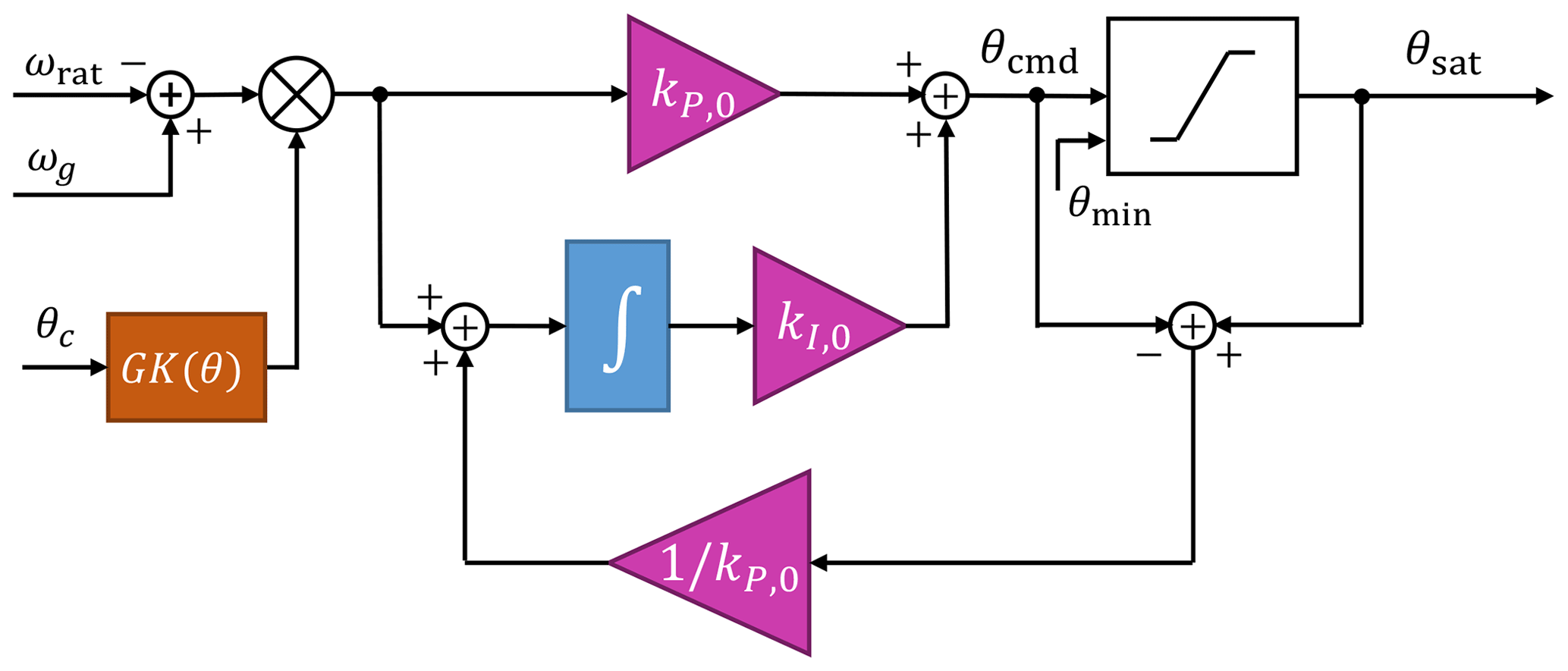
Figure A1 Proportional–integral control with antiwindup scheme used for above-rated control. The difference between the pitch control set point ω_rat and the generator speed ω_g is multiplied with the gain-correction factor GK(θ_avg), which is a function of the current collective blade pitch θ_c. The proportional–integral gains at zero pitch, k_P,0 and k_I,0, are derived in Eqs. (A15) and (A16). The pitch command θ_cmd is saturated to some minimum pitch setting θ_min and the output θ_sat is the input to the blade pitch actuator.

By defining a new state, $\dot{\mathit{\varphi }}=\mathit{\delta }{\mathit{\omega }}_{\mathrm{g}}$, and combining Eqs. (A2), (A3), and (A4), the generator speed dynamics are

$$\begin{array}{}\text{(A5)}& J_{\mathrm{tot}}\ddot{\mathit{\varphi }}+{\displaystyle \frac{\mathrm{1}}{{\mathit{\omega }}_{\mathrm{rat}}}}\left(-{\displaystyle \frac{\partial P}{\partial \mathit{\theta }}}\right)k_P{G}^{\mathrm{2}}\dot{\mathit{\varphi }}+{\displaystyle \frac{\mathrm{1}}{{\mathit{\omega }}_{\mathrm{rat}}}}\left(-{\displaystyle \frac{\partial P}{\partial \mathit{\theta }}}\right)k_I{G}^{\mathrm{2}}\mathit{\varphi }=\mathrm{0},\end{array}$$

which can be represented by a second-order dynamic system in the form of

$$\begin{array}{}\text{(A6)}& M_{\mathrm{reg}}\ddot{\mathit{\varphi }}+D_{\mathrm{reg}}\dot{\mathit{\varphi }}+K_{\mathrm{reg}}\mathit{\varphi }=\mathrm{0},\end{array}$$

where M_reg, D_reg, and K_reg are the mass, damping, and stiffness of the regulator mode, respectively. Alternatively, the regulator mode can be represented by its natural frequency ω_reg and damping ratio ζ_reg, defined by

$$\begin{array}{}\text{(A7)}& {\mathit{\omega }}_{\mathrm{reg}}=\sqrt{{\displaystyle \frac{K_{\mathrm{reg}}}{M_{\mathrm{reg}}}}}\mathrm{and}{\mathit{\zeta }}_{\mathrm{reg}}={\displaystyle \frac{D_{\mathrm{reg}}}{\mathrm{2}{\mathit{\omega }}_{\mathrm{reg}}{M}_{\mathrm{reg}}}}.\end{array}$$

By defining the desired properties of the generator speed dynamics, ω_reg and ζ_reg, the proportional and integral gains are defined as follows:

$$\begin{array}{}\text{(A8)}& k_P={\displaystyle \frac{\mathrm{2}{J}_{\mathrm{tot}}{\mathit{\omega }}_{\mathrm{rat}}{\mathit{\omega }}_{\mathrm{reg}}{\mathit{\zeta }}_{\mathrm{reg}}}{G^{\mathrm{2}}\left(-\frac{\partial P}{\partial \mathit{\theta }}\right)}}\end{array}$$

and

$$\begin{array}{}\text{(A9)}& k_I={\displaystyle \frac{J_{\mathrm{tot}}{\mathit{\omega }}_{\mathrm{rat}}{\mathit{\omega }}_{\mathrm{reg}}^{\mathrm{2}}}{G^{\mathrm{2}}\left(-\frac{\partial P}{\partial \mathit{\theta }}\right)}}.\end{array}$$

A1.1 Power–pitch sensitivity and gain scheduling

Both the proportional Eq. (A8) and integral Eq. (A9) gains depend on the sensitivity of power to blade pitch

$$\begin{array}{}\text{(A10)}& {\displaystyle \frac{\partial P}{\partial \mathit{\theta }}}{|}_{\mathit{\theta }}=S\left(\mathit{\theta }\right),\end{array}$$

which we will define as S(θ) because it is a function of the blade pitch. Simulations in FAST are used to determine the pitch operating points at various above-rated wind speeds. The operating points are used in FAST linearizations, with all the degrees of freedom disabled, providing the input–output sensitivity from pitch to power. The results of performing this sensitivity analysis for several rotors are shown in Fig. A2.

Figure A2 Sensitivity of power to pitch used for gain scheduling the pitch controller for a selection of rotors in this article. The sensitivity values obtained from FAST linearizations are fit linearly and used to determine the gain-scheduling parameters for the pitch controller.

Because of the near-linear relationship with blade pitch θ, the sensitivity can be parameterized by

$$\begin{array}{}\text{(A11)}& S\left(\mathit{\theta }\right)=\left[{\displaystyle \frac{S\left(\mathrm{0}\right)}{{\mathit{\theta }}_k}}\right]\mathit{\theta }+S\left(\mathrm{0}\right)=S\left(\mathrm{0}\right)\left(\mathrm{1}+{\displaystyle \frac{\mathit{\theta }}{{\mathit{\theta }}_k}}\right),\end{array}$$

where S(0) is the sensitivity at θ=0^∘ and θ_k is the pitch angle at which the sensitivity doubles:

$$\begin{array}{}\text{(A12)}& S\left({\mathit{\theta }}_k\right)=\mathrm{2}S\left(\mathrm{0}\right).\end{array}$$

From simulation results like those in Fig. A2, the parameters in Eq. (A11) can be estimated; they are used to define the gain-correction factor

$$\begin{array}{}\text{(A13)}& \mathrm{GK}\left(\mathit{\theta }\right)={\displaystyle \frac{\mathrm{1}}{\mathrm{1}+\frac{\mathit{\theta }}{{\mathit{\theta }}_k}}}\end{array}$$

and the final, gain-scheduled PI gains:

$$\begin{array}{}\text{(A14)}& k_P=k_{P,\mathrm{0}}\mathrm{GK}\left(\mathit{\theta }\right)\mathrm{and}{k}_I=k_{I,\mathrm{0}}\mathrm{GK}\left(\mathit{\theta }\right),\end{array}$$

where

$$\begin{array}{}\text{(A15)}& k_{P,\mathrm{0}}={\displaystyle \frac{\mathrm{2}{J}_{\mathrm{tot}}{\mathit{\omega }}_{\mathrm{rat}}{\mathit{\omega }}_{\mathrm{reg}}{\mathit{\zeta }}_{\mathrm{reg}}}{G^{\mathrm{2}}\left[-S\left(\mathrm{0}\right)\right]}}\end{array}$$

and

$$\begin{array}{}\text{(A16)}& k_{I,\mathrm{0}}={\displaystyle \frac{J_{\mathrm{tot}}{\mathit{\omega }}_{\mathrm{rat}}{\mathit{\omega }}_{\mathrm{reg}}^{\mathrm{2}}}{G^{\mathrm{2}}\left[-S\left(\mathrm{0}\right)\right]}}.\end{array}$$

Figure A1 depicts the implementation in block diagram form.

A1.2 Summary of pitch control tuning procedure

To derive the parameters from simulations and tune the regulator mode, we use the following procedure:

1. Simulate the operating points in FAST using a steady wind input across above-rated wind speeds. Choose a S(0) so that the PI gains produce a stable result. Simulate for enough time for the values to reach steady state and record the blade pitch at each wind speed.

2. Linearize the turbine in FAST, disabling all of the degrees of freedom, at the wind speeds and pitch angles found from the previous step. Use the element of the input–output matrix that corresponds to the pitch input and power output matrix to determine the sensitivity of power to pitch at the various pitch angle operating points. Plot the values and fit the parameters S(0) and θ_k as in Fig. A2.

3. Tune the regulator mode (ω_reg,ζ_reg) using the desired design measure. Usually, larger natural frequencies (ω_reg) result in better generator regulation but also higher structural loads. A grid search could be used or an optimization procedure like the one in Sect. 3.2.

Appendix B: Turbine model summary

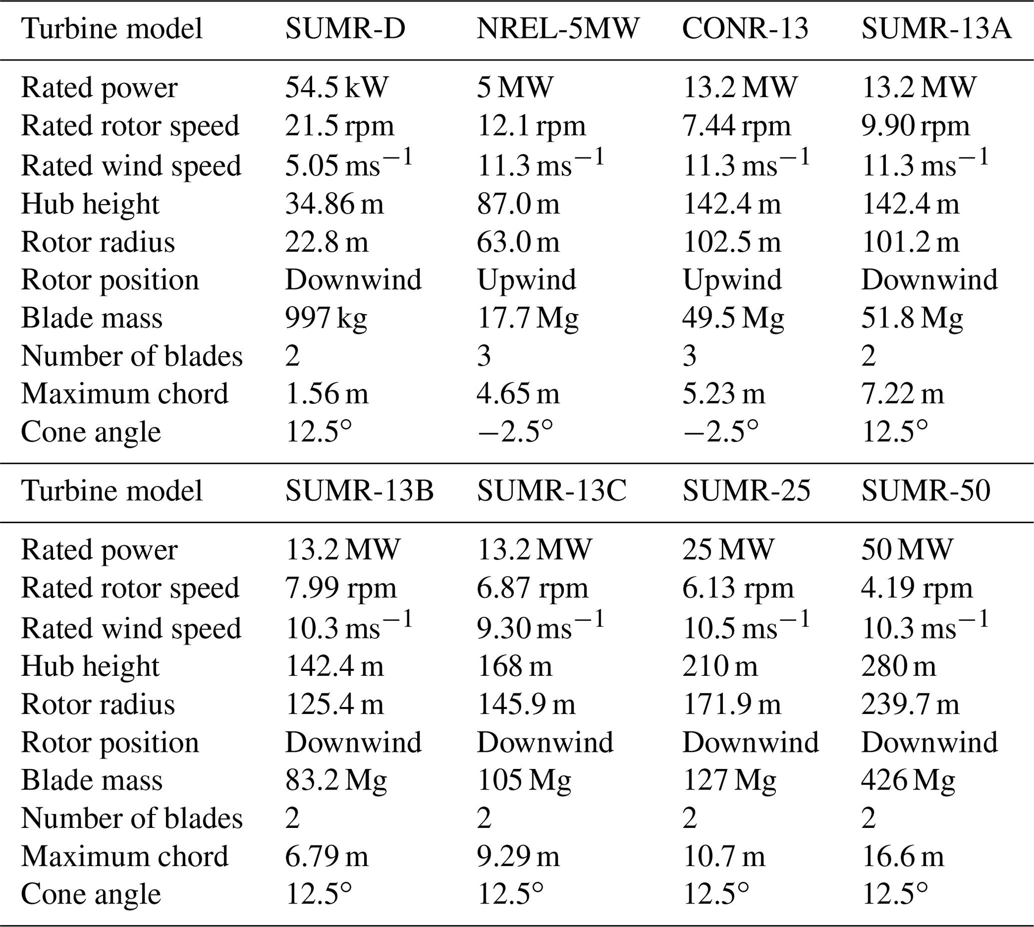
The turbine models summarized in Table B1 were used to perform the control tuning optimization procedures detailed in this article.

Table B1 Summary of turbine models used in this study.