The most similar predictor – on selecting measurement locations for wind resource assessment

We present the “most similar” method for selecting optimal measurement positions for wind resource assessment.

Wind resource assessment is generally done by extrapolating a measured and long-term corrected wind climate at one location to a prediction location using a micro-scale flow model. If several measurement locations are available, standard industry practice is to make a weighted average of all the possible predictions using inverse-distance weighting. The most similar method challenges this practice. Instead of weighting several predictions, the method only selects the single measurement location evaluated to be most similar.

We validate the new approach by comparing against measurements from 185 met masts from 40 wind farm sites and show improvements compared to inverse-distance weighting. Compared to using the closest measurement location, the error of power density predictions is reduced by 13 % using inverse-distance weighting and 34 % using the most similar method.

1 Introduction

When assessing the energy potential of a new wind farm, a crucial step is to predict the mean wind climate at each wind turbine position. The conventional approach for predicting the wind climate is to erect a meteorological mast (met mast) at a nearby location and extrapolate the measured wind climate to every wind turbine position using a micro-scale flow model (MEASNET procedure, 2016). The flow model estimates how the surrounding topography perturbs the wind and can thereby predict the wind climate at each wind turbine position. Much research focuses on the development of improved micro-scale models; however, this work focuses on optimal met mast positioning and on how this improves predictions irrespectively of the chosen micro-scale model.

This introduction will first explain that met masts today are positioned to minimize the distance to wind turbine positions. We then present a hypothesis that states that met masts should instead be placed following the “similarity principle”, and finally, the section describes how the hypothesis will be tested.

1.1 The representativeness radius

The distance between the measurement and prediction location is traditionally used as an indicator of model uncertainty, and measurement campaigns are often planned to minimize the extrapolation distance. MEASNET procedure (2016) defines a “representativeness radius” as the distance from a met mast to the furthest location that can be extrapolated with tolerable uncertainty. The representativeness radius depends on the complexity of the terrain, where complex terrain is characterized by having terrain slopes greater than 0.3. Figure 1 illustrates two met masts located in hilly terrain. Following the recommendations of MEASNET procedure (2016) for simple and complex terrain, the measurements taken in the valley, U₀₁, are preferable for predicting U_P as the distance is small. For sites that are even more complex, MEASNET states that mast positioning should be based on a site-specific analysis.

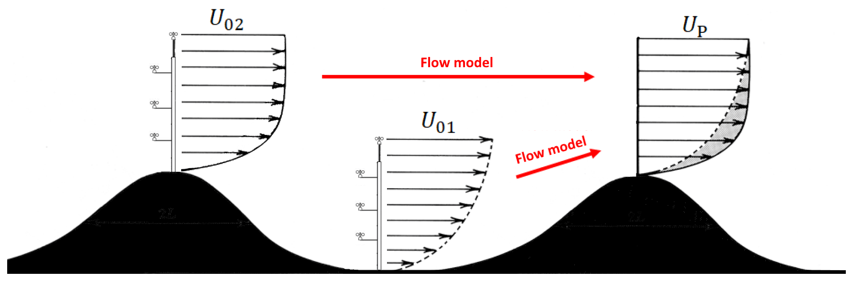
Figure 1 The figure illustrates how a measured wind climate can be extrapolated to a prediction site using a flow model. Following the “representativeness radius”, the model error is reduced when the distance between met mast and prediction location is minimized; accordingly met mast 1 (U₀₁) is the preferred predictor. Following “the similarity principle” model errors are reduced when the wind conditions at the met mast and the predicted location are similar; accordingly met mast 2 (U₀₂) is preferable despite its more distant location.

1.2 The similarity principle

According to Landberg et al. (2003), errors related to flow modelling are minimized when the predictor site (the met mast location) and the predicted site (the wind turbine location) are as “similar” as possible regarding factors like regional wind climate, roughness, orography and obstacles. Landberg et al. (2003) refers to this as the similarity principle. The underlying assumption is that no matter how advanced a flow model, it always produces errors, and they scale with the forcing applied. Figure 1 illustrates the similarity principle. The wind conditions in the valley, U₀₁, differ substantially from the conditions at the prediction site, U_P, and a better predictor (according to the similarity principle) is, therefore, the hilltop met mast, U₀₂, despite its more distant location.

1.3 The most similar predictor

Experienced wind and site engineers determine suitable locations for met masts based on the representativeness radius and their judgement. They intuitively understand that distance is not the only parameter that should be evaluated; however, since no algorithmic method for similarity exists, the industry standard is often to minimize the extrapolation distance.

To make a parameter that represents similarity, we define the directional-averaged speedup uncertainty, σ_S,

$$\begin{array}{}\text{(1)}& {\mathit{\sigma }}_{\mathrm{S}}^{\mathrm{2}}=\sum _{j=\mathrm{1}}^{N_{\mathit{\theta }}}{f}_j{\mathit{\sigma }}_{{\mathrm{S}}_j}^{\mathrm{2}},\end{array}$$

where f_j is the wind direction frequency at the met mast, N_θ is the number of wind direction sectors and ${\mathit{\sigma }}_{{\mathrm{S}}_j}^{\mathrm{2}}$ is the speedup uncertainty of the micro-scale model. As an expression for the speedup uncertainty for a particular wind direction, we use the model by Clerc et al. (2012):

$$\begin{array}{}\text{(2)}& {\mathit{\sigma }}_{{\mathrm{S}}_j}^{\mathrm{2}}={\left(\mathit{\lambda }\left[\mathrm{1}-\exp \left({\displaystyle \frac{-d}{L_{\mathrm{1}}}}\right)\right]\right)}^{\mathrm{2}}+{\left|{\displaystyle \frac{S_j-\mathrm{1}}{S_j+\mathrm{1}}}\right|}^{\mathrm{2}},\end{array}$$

where d is the extrapolation distance, L₁=1 km and λ=0.1 are empirically calibrated constants (Clerc et al., 2012), and $S_j=U_{{\mathrm{P}}_j}/U_{{\mathrm{0}}_j}$ is the speedup where U₀ and U_P are the measured and predicted mean wind speeds respectively. L₁ and λ have not been re-calibrated in this work but are kept to their original values.

σ_S combines into one expression, the uncertainty associated with both extrapolation distance and the wind speed difference. Small values of σ_S signify that predictor and prediction conditions are similar. The inclusion of speedup in the expression ensures that any difference between predictor and prediction site included in the micro-scale flow model is evaluated (roughness, orography, obstacles, measurement height, etc.). The speedup uncertainty is, therefore, expected to be a more accurate “measure of similarity” than distance, and we define the “most similar” predictor to be the location with the smallest σ_S value.

1.4 Multi-mast strategies

For large wind farms with several met masts, a standard practice when making predictions is to either select the closest available predictor or to make a weighted average of multiple predictions using “inverse-distance weighting”. As an example, the inverse-distance-weighted mean wind speed, U_P, can be determined as

$$\begin{array}{}\text{(3)}& U_{\mathrm{P}}={\displaystyle \frac{\sum _{i=\mathrm{1}}^{N_M}{W}_i{U}_{{\mathrm{P}}_i}}{\sum _{i=\mathrm{1}}^{N_M}{W}_i}},\end{array}$$

where $U_{{\mathrm{P}}_i}$ is the predicted mean wind speed, $W_i=d_i^{-\mathrm{2}}$ is the predictor weight, d_i is the extrapolation distance and N_M is the number of predictors on a particular site. The underlying reason for using inverse-distance weighting is that the standard error of a weighted mean decreases with the number of independent predictions. However, for this to be valid, the predictions are assumed independent (model errors should be random), and extrapolation distance is assumed to be the parameter that correlates the strongest with model error.

This paper aims to show that met masts should be placed following the similarity principle instead of reducing extrapolation distance. The hypothesis is verified by showing that the most similar predictor gives lower prediction errors than the closest predictor and inverse-distance weighting. In the following, we conduct a large number of predictions using the following multi-mast strategies and compare the results to measurements.

$$\begin{array}{}\text{(4)}& {\displaystyle }& {\displaystyle }\mathrm{Closest}\mathrm{predictor}:W_i=\left\{\begin{array}{cl}\mathrm{1}& \mathrm{if}{d}_i=\min \left(d\right)\\ \mathrm{0}& \mathrm{otherwise}\end{array}\right.\text{(5)}& {\displaystyle }& {\displaystyle }\mathrm{Inv}.\mathrm{dist}.\mathrm{weighting}:W_i=d_i^{-\mathrm{2}}\text{(6)}& {\displaystyle }& {\displaystyle }\mathrm{Most}\mathrm{similar}\mathrm{predictor}:W_i=\left\{\begin{array}{cl}\mathrm{1}& \mathrm{if}{\mathit{\sigma }}_{{\mathrm{S}}_i}=\min \left({\mathit{\sigma }}_{\mathrm{S}}\right)\\ \mathrm{0}& \mathrm{otherwise}\end{array}\right.\end{array}$$

2 Validation method

To validate the usefulness of the most similar predictor, we compare the performance of the three multi-mast strategies against wind measurements. Sites with at least three met masts are used in the comparison. The multi-mast sites allow for predictions with multiple predictors and provide an objective way to evaluate the strategies. The validation method consists of three steps described in detail in the following sections:

1. wind measurements – preparation of the wind data for the flow model,

2. flow model – prediction of all mast locations using every other mast as a predictor,

3. prediction statistics – calculation of mean wind speed and power density using each multi-mast strategy.

The wind measurements and flow model setups are identical for each multi-mast strategy; only the mast weights, W_i, used for calculating the wind statistics are different to allow for a simple and objective evaluation.

2.1 Wind measurements

The dataset used in this work has been collected specifically to validate multi-mast strategies. It is obtained through wind project developers worldwide and is considered to cover a wide spectrum of the conditions experienced in wind projects. The dataset consists of wind measurements from sites with three or more met masts. By having at least three masts, each mast location can be predicted using at least two predictors, and results can be compared against the measurements taken at the predicted mast.

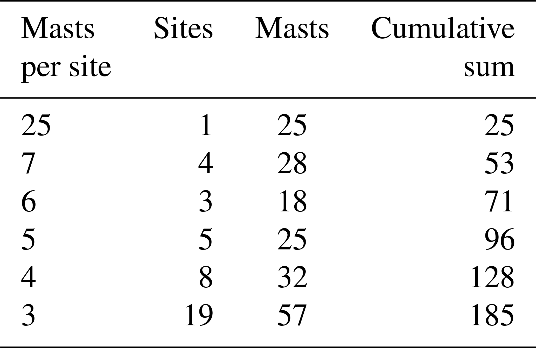
The dataset consists of wind speed and wind direction measured from the top anemometer of each met mast, already screened and long-term corrected by wind project developers. The data are grouped into 36 10^∘ wind direction sectors and have Weibull distributions fitted to the wind speed histogram. Wind statistics from a total of 210 met masts were provided for the study. The only additional screening that has been conducted is the removal of four sites (25 met masts) from the dataset. These sites were removed since mast-to-mast predictions of wind speed and power density led to substantial errors (>3σ) for four of the met masts. We did not investigate the reason for the significant errors but removed the sites from the investigation. Table 1 shows a summary of the sites and met masts used. As seen, the screened data consist of 185 met masts distributed over 40 wind turbine sites.

Table 1 Number of met masts used for the study.

The data come from met masts located near potential wind energy installations, and the 185 mast locations represent varied site conditions from all over the world. Figure 2 illustrates the complexity of the sites using the RIX (left) and ΔRIX (right) measures where RIX is defined by the percentage fraction of the terrain along the prevailing wind direction, which is over a critical slope of 0.3 (Bowen and Mortensen, 2004). The mean RIX value is 7.0 %, which can be considered moderately complex terrain. Compared to the closest neighbouring mast, 84 masts have $\left|\mathrm{\Delta }\mathrm{RIX}\right|$ values of less than 1 % and 164 masts have $\left|\mathrm{\Delta }\mathrm{RIX}\right|$ below 5 %. Most of the met masts are therefore placed in similar, well-exposed hills and ridges.

Figure 2 RIX and $\left|\mathrm{\Delta }\mathrm{RIX}\right|$ for all 185 met masts. $\left|\mathrm{\Delta }\mathrm{RIX}\right|$ is calculated using the closest neighbouring mast.

Figure 3 Mast height and distance to the closest neighbouring mast for all 185 met masts.

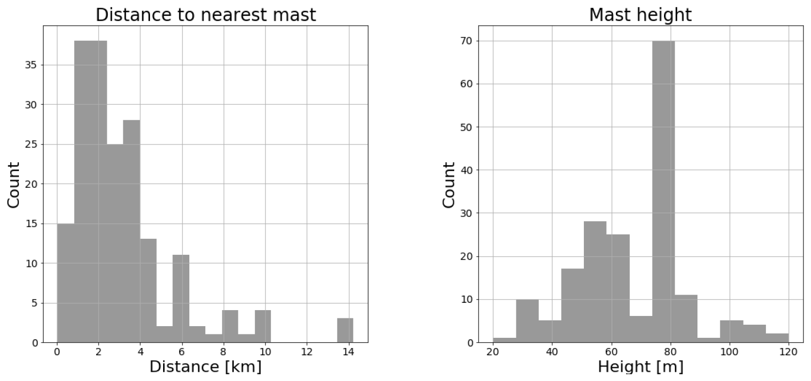
Figure 3 shows the height of the masts (right) and the distance to their closest neighbour (left). The distance is up to 10 km, but on average the distance is 3.1 km. As seen, the masts do not have the same height but vary from 20 to 120 m, and half of the sites have mast height variations. These sites often have combinations of short and tall masts, e.g. of 40∕80, 60∕80 or 60∕100 m masts. The wind statistics have not been corrected or “sheared up” to unify the height differences. Instead, the flow model has been used directly to estimate the wind statistics at the prediction height using the statistics at the predictor height. The most similar method has an advantage compared to the other multi-mast strategies for sites with different mast heights as there will be a speedup between masts of different heights and will therefore not be valued as similar. In the current analysis, this is however of minor importance as the results, particularly in Sect. 3.2, depend mainly on a single site with 25 met masts that are all 80 m tall.

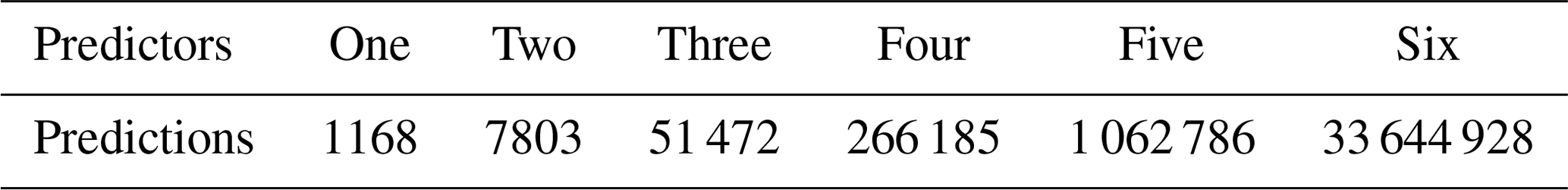
The dataset (Table 1) allows for a total of 185 possible predictions with two or more predictor masts. The results section analyses how the different multi-mast strategies perform with this specific mix of multi-mast sites. Also, other combinations of multi-mast sites from the same data pool have been made to analyse how the multi-mast strategies perform on sites with a specific number of predictor masts. As an illustration of how other multi-mast combinations can be made from the same data, we can imagine that a single site with three met masts can also be viewed as three different sites with two met masts. Table 2 shows the many combinations of predictions possible with one, two, three, four, five or six predictor masts. As seen, it is possible to make more than 33 million different predictions with six predictor masts. The many combinations are primarily possible because of the site that has 25 met masts. The results for different numbers of predictor masts are not directly comparable since they are based on different sites. The results section, therefore, normalizes the most similar and the inverse-distance-weighting results with the “closest mast” to make comparisons of the multi-mast strategies possible.

Table 2 Number of predictions possible for different numbers of predictors.

2.2 Flow model

The micro-scale flow model WAsP 12.3 (Troen and Petersen, 1989) has been used to make all wind climate predictions in this study. Since every mast location needs to be predicted using every possible predictor mast, there is a total of 1168 mast-to-mast predictions. A database and an automatic model script (PyWAsP) were made to conduct all the simulations, and every simulation was run with the standard WAsP 12.3 parameters. No ΔRIX or other corrections have been made to the model results, and no tuning of model parameters to improve results was performed.

The topography maps used for the flow model were provided to the authors and used directly without corrections or quality control. As all data have previously been analysed to be used for wind farm development, and scrutinized by third-party companies, the data are considered to have an industry standard quality. The current work is a statistical analysis of the multi-mast strategies. All simulations are based on identical model setups and using the digitized maps, mast locations, anemometer heights and wind measurements provided to the authors; only the method used to calculate the predicted wind statistics is different between the three multi-mast strategies.

2.3 Predicted wind statistics

Wind statistics are calculated at each prediction location to validate the performance of the multi-mast strategies. Specifically, the predicted mean wind speed, U_P (m s⁻¹), and mean power density, E_P (W m⁻²), are compared to the measured values (U₀ and E₀). Since the measured wind data and the wind climate predictions are given in terms of the Weibull parameters A and k, the mean wind speed and mean power density are calculated following Troen and Petersen (1989):

$$\begin{array}{}\text{(7)}& {\displaystyle }& {\displaystyle }{U}_i=\sum _{j=\mathrm{1}}^{N_{\mathit{\theta }}}{f}_j{A}_{ij}\mathrm{\Gamma }\left(\mathrm{1}+{\displaystyle \frac{\mathrm{1}}{k_{ij}}}\right),\text{(8)}& {\displaystyle }& {\displaystyle }{E}_i={\displaystyle \frac{\mathrm{1}}{\mathrm{2}}}\mathit{\rho }\sum _{j=\mathrm{1}}^{N_{\mathit{\theta }}}{f}_j{A}_{ij}^{\mathrm{3}}\mathrm{\Gamma }\left(\mathrm{1}+{\displaystyle \frac{\mathrm{3}}{k_{ij}}}\right),\end{array}$$

where ρ is air density (1.225 kg m⁻³) and Γ is the gamma function. Having calculated the wind speed and power density for every possible single-mast prediction, the multi-mast strategies were applied to calculate the final predicted wind statistics:

$$\begin{array}{}\text{(9)}& {\displaystyle }& {\displaystyle }{U}_{\mathrm{P}}={\displaystyle \frac{\sum _{i=\mathrm{1}}^{N_M}{W}_i{U}_{{\mathrm{P}}_i}}{\sum _{i=\mathrm{1}}^{N_M}{W}_i}},\text{(10)}& {\displaystyle }& {\displaystyle }{E}_{\mathrm{P}}={\displaystyle \frac{\sum _{i=\mathrm{1}}^{N_M}{W}_i{E}_{{\mathrm{P}}_i}}{\sum _{i=\mathrm{1}}^{N_M}{W}_i}},\end{array}$$

where W_i is the mast weight that depends on the chosen strategy (Sect. 1.4). It was also considered to apply a generic wind turbine power curve to allow calculation of energy yield predictions. However, as the prediction heights and wind speeds vary between the sites, using a single power curve for all predictions was not pursued.

2.4 Evaluation method

To evaluate the multi-mast strategies, we compare the measured and predicted wind statistics at each mast position and calculate the average error of all predictions. The closest-mast results are used as a baseline. The paper does not analyse the baseline error in any detail; instead, the paper focuses on how the multi-mast strategies improve the baseline. The data and model setup used for the closest mast, inverse-distance weighting and most similar methods are identical, to make an objective comparison of the multi-mast strategies. For each multi-mast strategy, the absolute error of each mast prediction is given by

$$\begin{array}{}\text{(11)}& X_i=X_{\mathrm{P}}-X_{\mathrm{0}},\end{array}$$

where X_P is either the predicted mean wind speed (U_P) or power density (E_P) and X₀ is the measured value (U₀ or E₀). The mean error of a strategy is calculated by

$$\begin{array}{}\text{(12)}& \mathit{\mu }={\displaystyle \frac{\sum _{i=\mathrm{1}}^n{X}_i}{n}},\end{array}$$

where n is the number of mast predictions. Finally, the standard deviation of the error is given by

$$\begin{array}{}\text{(13)}& \mathit{\sigma }=\sqrt{{\displaystyle \frac{\sum _{i=\mathrm{1}}^n{\left(X_i-\mathit{\mu }\right)}^{\mathrm{2}}}{n-\mathrm{1}}}}.\end{array}$$

The results shown in the following indicates the mean error, μ, the standard deviation of the errors, σ, and the number of predictions used to calculate the statistics, n.

3 Results

3.1 Original sites

The top row of Fig. 4 shows histograms of the absolute error of wind speed (left) and power density (right) for each of the 185 mast predictions using closest mast as a multi-mast strategy. Gaussian distributions are shown on the histograms (despite the poor fit), and the mean error and standard deviation of wind speed (μ=0.11, σ=0.63) and power density (μ=36.3, σ=149) are given in the legends. The observed mean wind speed and power density of the 185 masts are 7.36 m s⁻¹ and 460.7 W m⁻² respectively.

Figure 4 Histograms of the absolute wind speed (a, c, e) and power density (b, d, f) error when using the closest mast (a, b), inverse-distance weighting (c, d) and most similar (e, f) strategies. The mean bias and standard deviations are given in the legend. All 185 mast positions have been predicted to make this figure.

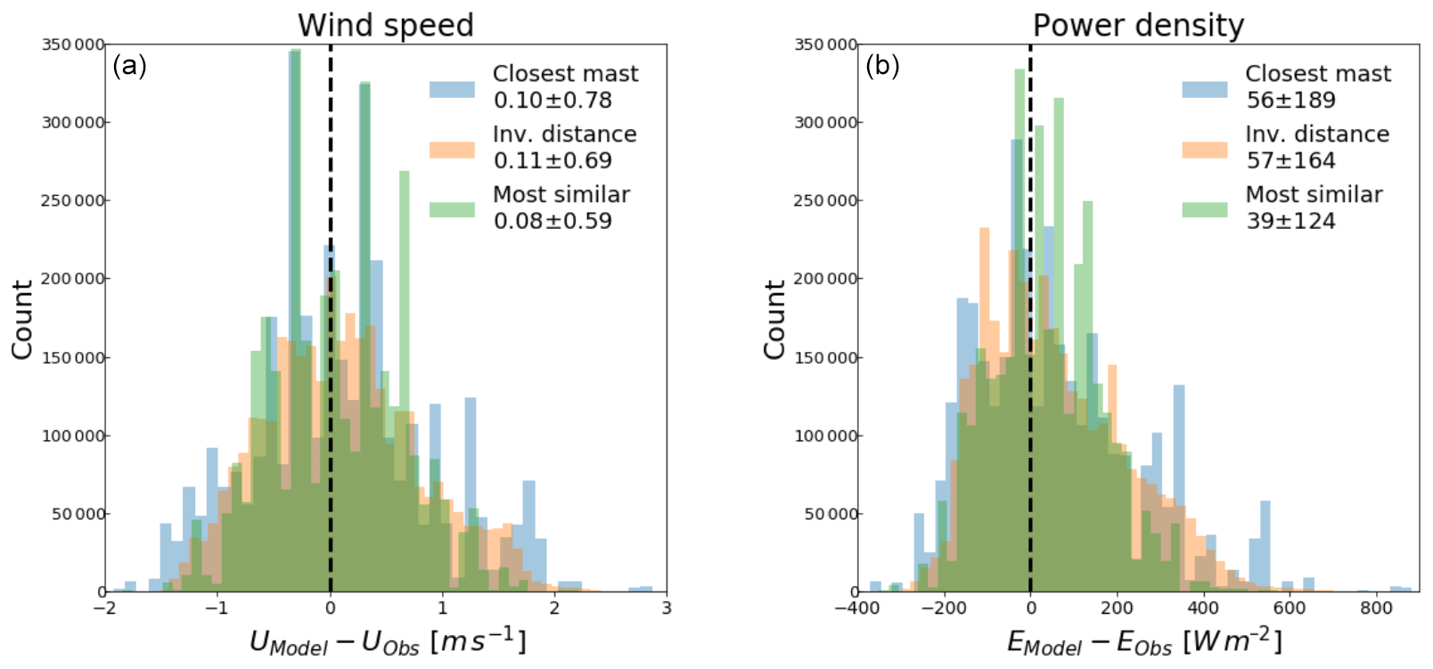
Figure 5 Histograms of the absolute wind speed (a) and power density (b) error for different combinations of prediction location and six predictor masts using the three different multi-mast strategies. Each histogram consists of more than 33 million predictions.

The results for inverse-distance weighting and most similar predictor are shown in the middle and bottom rows of Fig. 4. The left column shows that both multi-mast strategies significantly reduce both the mean wind speed error and the standard deviation compared to the closest mast. The standard deviation of the wind speed error is seen to decrease from 0.63 to 0.54 m s⁻¹ for both methods. The right column of the figure shows even more substantial error reductions for power density. The standard deviation of power density decreases from 149 to 125 W m⁻² for inverse-distance weighting and from 149 to 116 W m⁻² for most similar mast. Therefore, by selecting the most similar location, the mean power density error is reduced by 22 % compared to the closest mast and 7 % compared to inverse-distance weighting.

3.2 New predictor combinations

To clarify the difference between strategies that rely on the representativeness radius (closest mast and inverse-distance weighting) and the similarity principle (most similar predictor), this section focuses on sites with a specific number of predictor masts. By combining the available dataset, it is possible to generate new combinations of sites with one, two, three, four, five or six predictors (see Table 2).

As an example of the absolute prediction errors, Fig. 5 shows a histogram of the absolute error of wind speed (left) and power density (right) for predictions that use six predictors. The available dataset allows 33 million different combinations of a prediction location and six predictor masts. The histograms of the strategies have different colours, and the legends indicate the mean error and the standard deviation of each. Compared to the closest mast, the standard deviation of power density decreases from 189 to 164 W m⁻² for inverse-distance weighting and from 189 to 124 W m⁻² for the most similar mast.

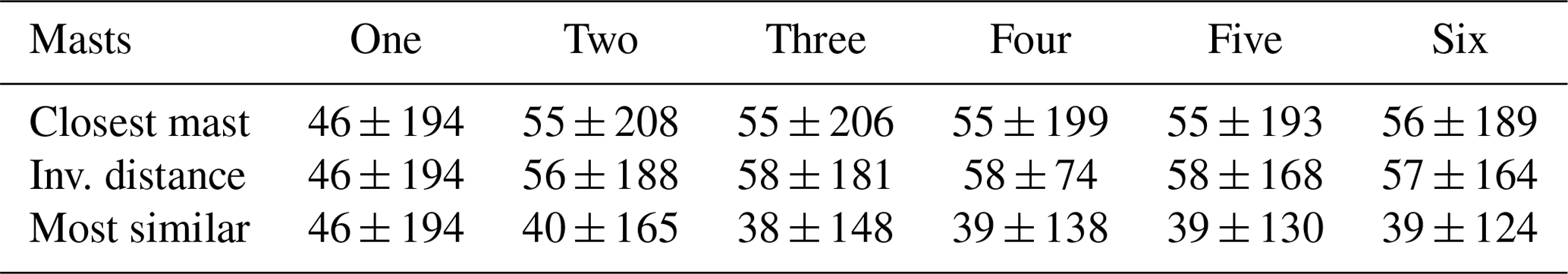
The mean absolute error and the standard deviation for predictor combinations with one, two, three, four, five and six predictor masts are given in Tables A1 and A2; however, the results are not directly comparable since they are based on different sites. To make a more valid comparison, we normalize all the results with the results of the closest mast. Figure 6 shows the normalized average reduction in the standard deviation of wind speed error (left) and power density error (right) for inverse-distance weighting and the most similar predictor compared to the closest mast. Note that the multi-mast strategies give identical results for predictions with only one predictor.

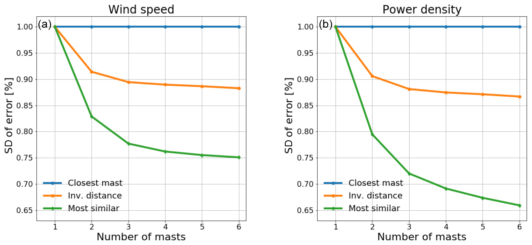
Figure 6 Reduction of the standard deviation of wind speed (a) and power density (b) error as function of predictor masts when using inverse-distance weighting and the most similar predictor compared to closest mast.

Figure 6 shows that both inverse-distance weighting and most similar predictors significantly reduce the average prediction error compared to the closest mast. While inverse-distance weighting reduces the error significantly with two predictors compared to one, the added improvement of using three or more predictor masts is much smaller. The most similar strategy has achieved 34 % reduction of the standard deviation of power density error with six predictor masts, and it appears that the error would keep decreasing with additional predictor masts. It should be noted that the most similar strategy only uses a single predictor mast, but having more options to choose from decreases the error. This indicates that significant improvements are gained if the most similar strategy is followed for placement of met masts, and it should also be used for single-met-mast campaigns.

4 Conclusions

We have presented a novel method for determining the most similar measurement location for wind resource assessment using an expression of the direction-averaged speedup uncertainty. Based on measurements from 185 met masts, the most similar met mast is on average a better predictor than the closest mast and inverse-distance weighting. This provides strong evidence in favour of the hypothesis that met masts should be positioned according to the similarity principle instead of reducing the distance to the wind turbines.

The met masts used in this study have all been positioned by experienced wind and site engineers on well-exposed ridges, and 164 of the 185 met masts have $\left|\mathrm{\Delta }\mathrm{RIX}\right|$ values below 5 %. In the traditional view, this would mean that the closest predictor and the predicted location on average should have similar wind conditions. Despite this, substantial improvements (36 % uncertainty reduction on power density predictions) were found by selecting the most similar predictor. This also indicates that even larger error reductions are possible if resource measurement campaigns are designed from the start using the most similar methodology, especially for single-met-mast campaigns. Designing an optimal measurement campaign using the most similar methodology requires a micro-scale flow model, a wind turbine layout and an indication of the main wind directions. With these tools, the direction-averaged speedup uncertainty for all wind turbine positions can be calculated and minimized.

The industry standard is often to use inverse-distance weighting for resource assessment; the underlying reason is that the standard error of a weighted mean decreases with the number of independent predictions. Troen and Hansen (2015) show that the average of two independent flow models does decrease the uncertainty; however, predictions that use the same flow model and measurements from the same period are not independent. The reason why inverse-distance weighting improves compared to the closest mast is probably that it “repairs” a poor choice of predictor mast. Weighted results using inverse “direction-averaged speedup uncertainty” as predictor weight have also been tried (not shown); however, results do not improve compared to the most similar predictor. To optimally combine the solution from several masts, it is necessary to consider the correlation of the errors (Clerc et al., 2012), which is not trivial. The most similar predictor is a practical alternative.

Appendix A

Table A1 Wind speed error (mean and standard deviation) depending on the number of predictor masts and selected strategies.

Table A2 Power density error (mean and standard deviation) depending on the number of predictor masts and selected strategies.