Investigations of aerodynamic drag forces during structural blade testing using high-fidelity fluid–structure interaction

Aerodynamic loads need to be known for planning and defining test loads beforehand for wind turbine blades that are tested for fatigue certifications. It is known that the aerodynamic forces, especially drag, are different for tests and operation, due to the entirely different flow conditions. In test facilities, a vibrating blade will move in and out of its own wake, increasing the drag forces on the blade. This is not the case in operation. To study this special aerodynamic condition present during experimental tests, numerical simulations of a wind turbine blade during pull–release tests were conducted. High-fidelity three-dimensional computational fluid dynamics methods were used throughout the simulations. In this way, the fluid mechanisms and their impact on the moving blade are clarified, and through the coupling with a structural solver, the fluid–structure interaction is studied. Results are compared to actual measurements from experimental tests, verifying the approach. It is found that the blade experiences a high drag due to its motion towards its own whirling wake, resulting in an effective drag coefficient of approximately 5.3 for the 90^∘ angle of attack. This large drag coefficient was implemented in a fatigue test load simulation, resulting in a significant decrease in bending moment along the blade, leading to less load being applied than intended. The confinement from the test facility did not impact this specific test setup, but simulations with longer blades could possibly yield different conclusions. To the knowledge of the authors, this investigation, including three-dimensional effects, structural coupling and confinement, is the first of its kind.

1 Introduction

For a wind turbine blade to be certified, full-scale structural tests are required to ensure the blade strength and endurance against extreme and fatigue loads (Post, 2016). These tests are especially relevant, as wind turbine blade design optimization continuously moves the limit of what is possible in regards to saving material and lowering the levelized cost of energy (LCoE). When conducting fatigue tests on wind turbine blade designs, the standard procedure is to excite the blade in the resonance frequency for 2×10⁶–10×10⁶ cycles in flapwise and edgewise directions or both simultaneously using biaxial forcing (White, 2004; Greaves et al., 2011; Greaves, 2013; Post, 2016). Blades are usually anchored in a horizontal position by means of steel bolts connecting the root to a test rig, whereas the excitation is enforced using translating or rotating mass exciters or, more traditionally, by forced motions using ground-based hydraulic actuators. These dynamic tests usually take several months, as millions of cycles need to be done before the blade is approved for use in normal operation.

One measure that needs to be considered for fatigue testing in laboratories is that the tests are conducted at no wind flow conditions. This means that the aerodynamics around the vibrating blade are very different when compared to the conditions during operation. This can be seen in the high energy amount needed to conduct the fatigue tests, especially in the flapwise directions, where the aerodynamic damping is immense. The high aerodynamic damping is a result of vortices created around the vibrating blade. In a test facility with no air flow, these vortices are not quickly convected away from the blade, which they would be during wind turbine operation. This means that the blade has to travel back through the created vortices, resulting in a high air resistance to the motion, i.e., high aerodynamic damping.

A HAWC2-based (Larsen and Hansen, 2007) simulation tool was developed to simulate the dynamic response of the blade subject to test excitation and to determine the test setup, matching the fatigue target loads with the highest degree of accuracy. Test setups commonly include the installation of so-called tuning masses on yokes located at different radial positions along the blade to tune the blade test loads (Malhotra et al., 2012; Zhou et al., 2014). When using aeroelastic codes like HAWC2, FAST (Jonkman, 2005), FLEX4 (Øye, 1996), etc., for this calibration, the high aerodynamic damping is usually added by increasing the drag coefficients of the airfoils. This is needed, since codes based on Blade Element Theory (BET) aerodynamic models do not account for the vortices created. This phenomenon was studied by Greaves, who calibrated the drag coefficient to fit the drag force to two-dimensional computational fluid dynamics (CFD) simulations made by The National Renewable Energy Centre (Narec) in the UK (Greaves, 2013). The CFD study was limited to one airfoil, oscillating at 1 Hz in amplitudes of 1 and 2 m. In the study, Greaves found that a drag coefficient for a 90^∘ angle (flapwise motion) should be set to approximately 5.3 and 4.45 at 1 and 2 m amplitude, respectively, to account for the added damping. The drag coefficient for a 90^∘ angle on airfoils is, depending on the shape, usually in the range of 1.45 to 2.06 (Montgomerie, 1996; Post, 2016; Timmer, 2010), making this necessary increase quite significant. Despite not having enough cases to conclude the effect of amplitude and frequency, these factors might play a significant role in the creation of vortices and the effect thereof. The phenomenon seen is close to what was studied by Woolam at NASA back in 1968, where drag coefficients for oscillating flat plates were studied (Woolam, 1968). Here, experiments were conducted using a pendulum type apparatus with a flat plate attached, such that the damped oscillation due to air resistance was measured. It was found that oscillatory drag coefficients in general are larger than steady ones. Amplitude dependence was found only for small oscillations, where measurements were less accurate and independence of frequency was found (Woolam, 1968).

Confinement from walls, floor or ceiling was included neither in the aforementioned studies by Greaves (2013) using CFD nor in the experiments by Woolam (1968). In laboratories, the blades are positioned horizontally, and during fatigue tests they oscillate in a fashion that brings the blade tip close to the floor. The confinement of the laboratory might affect the aerodynamics around the tested blade. When the blade moves downwards, the air will be pushed down but blocked by the floor. If the confinement around the blade is sufficiently large, the build-up of pressure could affect it significantly.

In the present study, high-fidelity fluid–structure interaction (FSI) simulations of a pull–release test of a wind turbine blade were conducted to investigate three-dimensional effects of both the increased aerodynamic damping and the confinement effects. The investigation clarifies the aerodynamic phenomena that could be used for improving the traditional approach of handling the increased drag. Results are compared to actual experimental results found at the Large Scale Facility of DTU Wind Energy (Branner, 2020) to validate the FSI approach. Additionally, a preliminary numerical analysis for a single-axis flapwise fatigue test is presented, in which the test load evaluation is dependent on the choice of the drag coefficient C_D.

2 Methodology

In this section the numerical methods used will be presented, along with the test case and chosen model setup.

2.1 Numerical methods

2.1.1 Flow solver

The high-fidelity CFD code EllipSys3D (Michelsen, 1992, 1994; Sørensen, 1995) solves the incompressible Reynolds Averaged Navier–Stokes (RANS) and Large Eddy Simulation (LES) equations using the finite-volume method in general curvilinear coordinates, with a collocated grid arrangement. The code is parallelized using Message Passing Interface (MPI) and multi-block decomposition. EllipSys3D has multiple different convective schemes to choose from, e.g., Central Difference (CDS), Second-Order Upstream (SUDS), and Quadratic Upstream Interpolation for Convective Kinematics (QUICK). For pressure correction schemes, the SIMPLE algorithm and variations of this algorithm are used to couple the velocity and pressure. Rhie–Chow interpolation is used to avoid odd–even pressure decoupling.

Several turbulence models are implemented, such as two-equation RANS models and hybrid models like Detached Eddy Simulation (DES), Delayed DES (DDES), Improved DDES (IDDES), and higher-fidelity LES models.

Deformation of grids is handled through a moving mesh method with a volume blend factor, which moves mesh points according to their original displacement and distance to the blade surface along the grid line. This ensures that mesh points at the vicinity of the blade surface move along with the blade and that points further away only move a fraction of the displacement or not at all, by using a blending function. The code has been used thoroughly for many years for various cases and was validated in, e.g., the Mexico project (Bechmann et al., 2011; Sørensen et al., 2016) and for the Phase VI NREL rotor (Sørensen and Schreck, 2014; Sørensen et al., 2002).

2.1.2 Structural solver

HAWC2 (Larsen and Hansen, 2007) is an aeroelastic code widely used by industry. The structural part of the code is based on the multi-body formulation, accounting for nonlinear effects of large deflections. Each body can be represented by Euler or Timoshenko beam elements, which are connected with constraint equations to assemble the total structure.

The aerodynamics of HAWC2 are based on blade element momentum (BEM) theory and include multiple models that are capable of handling dynamic stall, tip loss effects, skewed inflow, etc. (Madsen et al., 2012). BEM-based models need input from airfoil polars along the blades to provide force coefficients used to calculate the aerodynamic forces.

2.1.3 FSI framework

The two codes are coupled, in a two-way manner, through the Python framework HAWC2CFD, originally created by Heinz (Heinz, 2013) and further developed by Horcas (González Horcas et al., 2019).

Using calculated displacements of nodes from HAWC2, the CFD mesh is deformed, and a new flow field is found through EllipSys3D. The loads predicted by the CFD solver are then fed back to the HAWC2 structure and a new deformation is found. A loosely coupled approach was found to be sufficient for wind-energy-related cases, due to the high mass ratio between the turbine and air (Heinz, 2013), and is therefore used.

In the remainder of this paper, the simulations conducted using this coupling with the CFD solver will be denoted as FSI-CFD. Simulations conducted using HAWC2 only will be referred to as FSI-BET.

2.2 Test case

In this investigation, pull–release tests of an approximately 14 m wind turbine blade were chosen, as experimental results were available for validation. The blade is designed for use on upwind horizontal axis turbines and equips a combination of FFA-W3 airfoils of varying thicknesses¹.

2.2.1 Experimental tests

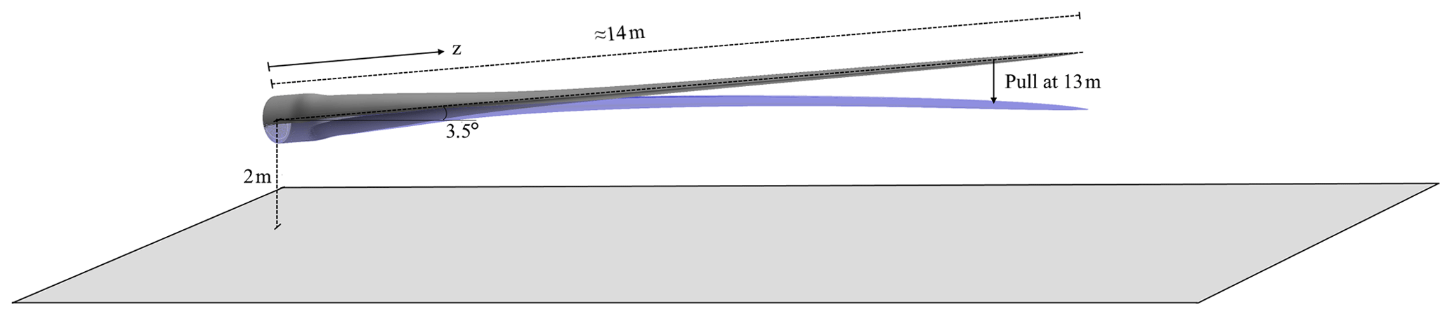
Actual pull–release tests of the studied wind turbine blade were conducted at the DTU Large Scale Facility at DTU Wind Energy Risø. For this experiment, the blade was cantilevered from the concrete test rig with a 3.5^∘ angle to the horizontal, with the pressure side facing upwards. Self-weight and dynamic loads were, therefore, acting in the flapwise load direction. Along the blade, multiple longitudinal electrical resistance strain gauges were placed with a resolution of approx. 0.5 m, and at 12.8 m, an accelerometer was attached to the pressure side of the blade and aligned with the middle axis of the spar cap. One unfortunate limitation of the used accelerometer was a measurable acceleration limit of ±4 G, which limits the measured oscillations of all the tests during the first oscillations after release. Acceleration measurements were shifted 1 G to compare with FSI-CFD results, which omitted gravity in the acceleration output (but not in calculations). In this way, the experimental measurements are in the range of −3 to 5 G.

At 13 m, a 4.8 kg saddle of timber was attached to the blade to enable the pull from beneath using a pulley system and a high-strength polyester rope, which was fastened to the strong floor of the facility and suddenly truncated to generate the free oscillation. In the present case, a pull ensuring a 600 mm tip displacement was chosen.

2.2.2 Modeled tests

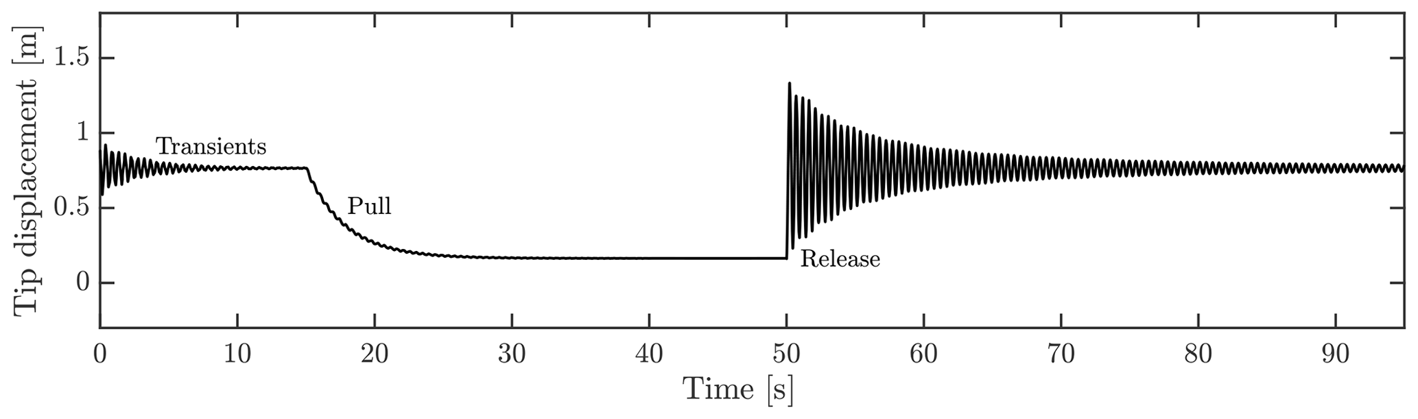
The control of the blade pull was done through HAWC2. A specific node on the blade at 13 m was pulled towards a node, representing the rope anchoring point at the floor. After the introduced vibrations were perished, the blade node was released, and the blade vibrated freely. This setup is similar to the actual experiment, where the saddle, attached at 13 m, was pulled towards the floor as sketched in Fig. 1. As an example of the simulations conducted, Fig. 2 shows the result of one case, which will be explained further in a later section. The figure depicts the vertical position of the node that was pulled and released. As has been shown, the initial 50 s was used to damp out transients and slowly pull the blade. After 50 s, the blade was released to vibrate freely for an additional 45 s.

Figure 1 Setup for the pull–release test and simulation.

Figure 2 The full simulation time series of tip displacement.

Multiple simulations were conducted on the DTU Wind Energy computer cluster “Jess”, which consists of 320 computer nodes, each with 20 Intel Xeon E5 2.8 GHz CPUs and 64 GB memory. To accelerate the computations, the grid sequencing of EllipSys3D was utilized, such that a very coarse grid was used in the FSI-CFD computations through the first 45 s of the simulations during the transients and pull. Along with this, the multigrid feature of EllipSys3D was enabled using five grid levels. Each full simulation took 80–130 h on 160 processors distributed on eight computer nodes. For FSI-BET simulations, each simulation took roughly 1 min to perform on one processor, which is 5 to 6 orders of magnitude lower than the FSI-CFD simulations.

Similar to the actual experiment, a pull resulting in 600 mm tip displacements from the equilibrium position of the blade was conducted, along with additional cases of 300, 400 and 500 mm to investigate any influence of initial amplitude. The 600 mm tip displacement will be used later on in this paper, unless otherwise stated.

Through the aerodynamic forces and velocity from the FSI-CFD simulations, the effective drag coefficient during the free oscillation was determined. The drag coefficient C_D was determined for the section at 12.8 m using peak values of force and velocity in the flapwise direction and using the quasi-steady aerodynamic force per unit length:

$$\begin{array}{}\text{(1)}& C_{\mathrm{D}}={\displaystyle \frac{\mathrm{2}{F}_{\mathrm{D}}}{\mathit{\rho }{v}^{\mathrm{2}}C}}.\end{array}$$

Here ρ is the air density set to 1.231 [kg m⁻²], C is the chord length (0.58 m at the specific node) and v is the effective relative air speed seen by the node.

Additionally, results of the FSI-CFD will be used for calibrations of drag coefficients to obtain equivalent FSI-BET results.

As the experiments were conducted indoor at the test facility, the modeled tests were performed with and without confining walls. In this way, it is possible to assess any influence of the confined space of an indoor closed test facility.

2.3 Model setup

2.3.1 Grid generation

The confining walls were created to resemble the actual dimensions of the facility but with several simplifications to facilitate grid generation; see Fig. 3. For boundaries, the facility walls, floor and ceiling were set as symmetry, with no flow perpendicular to the boundary and zero gradient tangentially. The blade surface was assigned a no-slip wall condition. To ensure stability in the code a velocity inlet and outlet region were created near the ceiling. The inflow was set to 0.1 m s⁻¹, which through initial studies (not shown here) was found to not influence the results.

Figure 3 Domain and boundaries of confined setup, resembling the test facility.

For the unconfined setup, a spherical domain was used with a radius of ≈25 blade lengths; see Fig. 5. Boundary conditions were velocity inlets for the majority of the boundary. An outlet based on the assumption of fully developed flow was applied to the downstream part of the boundary intersected by a cone with ±45^∘ angles from the center on the domain.

The inlet velocity was set to 0.1 m s⁻¹ for stability reasons, but this had no effect on the solution, as this velocity was much lower than the motion velocity of the blade during vibration.

The blade surface, depicted in Fig. 4, was created using an in-house Python tool based on the theoretical shape and discretized in 128 sections along the blade length and 256 cells chordwise, with nine grid points placed on the blunt trailing edge of the blade.

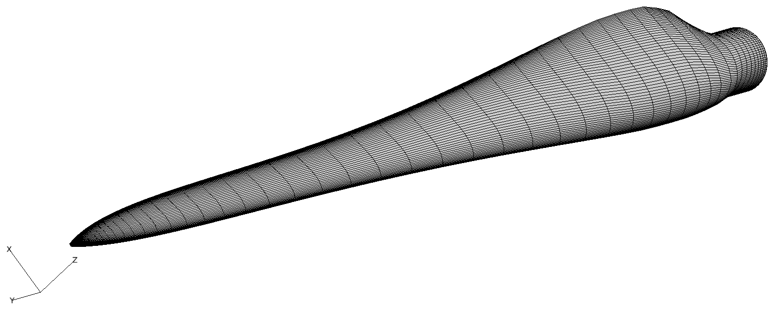
Figure 4 Surface mesh of the tested blade. Only every second line is shown for visual clarification.

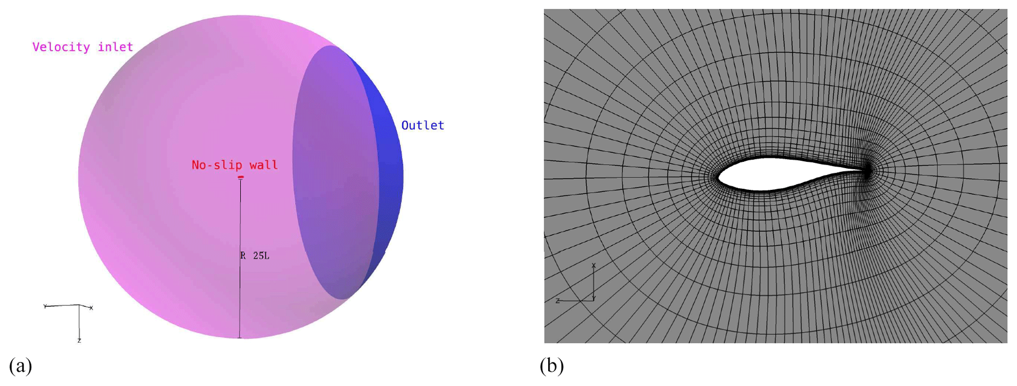
Figure 5 Spherical grid configuration: (a) outer boundary of grid and (b) extruded grid around airfoil. Only every second line is shown for visual clarification.

The non-confined grid was a regular hyperbolic grid structure, which was extruded from the blade surface using HypGrid3D (Sørensen, 1998), as seen in Fig. 5. A total of 5 242 880 mesh cells, divided into 160 blocks of $\mathrm{32}\times \mathrm{32}\times \mathrm{32}$, were used for the finest level of the spherical grid.

The grid generation of the confined setup was a combination of hyperbolic extrusion by Hypgrid3D from the blade surface, which was then connected to a transfinite mesh towards the confining walls using Pointwise 18.0 (Pointwise, 2017). A total of 5 177 344 mesh cells, divided into 158 blocks of $\mathrm{32}\times \mathrm{32}\times \mathrm{32}$, were used for the confined baseline grid; see Fig. 6.

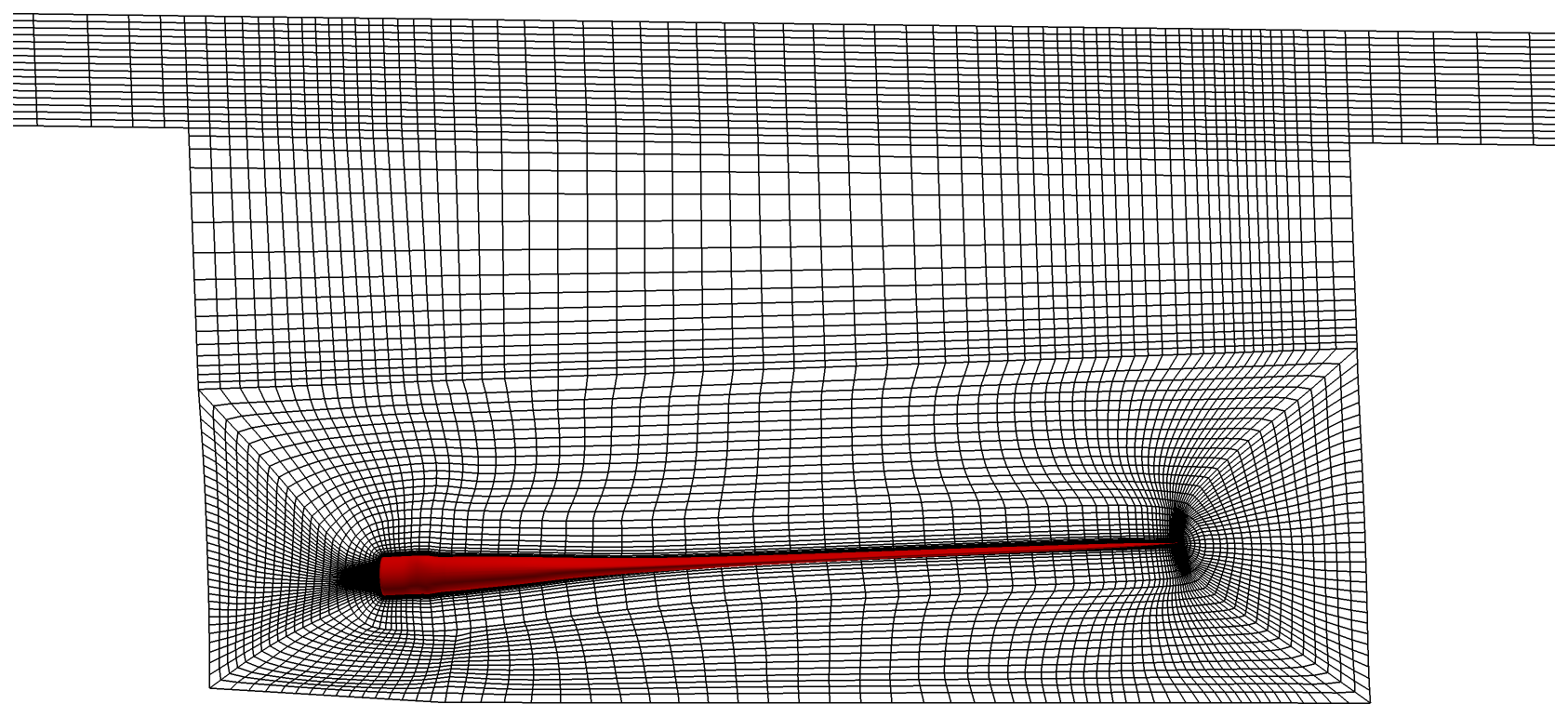
Figure 6 Volume mesh for the confined setup (shown as the computational surface at the midpoint). Only every second line is shown for visual clarification.

Grid sensitivity studies were made by coarsening (or refining) the grid, halving (or doubling) the number of grid points in each direction and doubling (or halving) the time step to keep a constant Courant number; see Sect. A1. The baseline and fine setups resulted in sufficiently similar forces on the blade, with only 0.41 % to −3.54 % force amplitude differences at the studied force peaks, and the baseline version of the grid was used throughout.

2.3.2 CFD setup

As mentioned above, the CFD code EllipSys3D was used for FSI-CFD simulations of the pull–release test. To solve the flow, the QUICK differencing scheme was used, along with a version of the SIMPLEC pressure correction scheme described in Shen et al. (2003). The time step sensitivity was studied, and it was found that time steps of $\mathrm{5}\times {\mathrm{10}}^{-\mathrm{4}}$ s were fine enough to obtain independent results; see Sect. A2.

Turbulence modeling was complicated by the fact that little or no flow was present in the test section. Results with RANS k−ω SST (Menter, 1993), DES k−ω (Spalart et al., 1997; Travin et al., 2004) and without turbulence models were compared. It was found that the turbulence models introduced only small differences in the resulting forces on the blade but made the computations unstable, probably due to the no flow condition around the blade; see Sect. A3. For this reason, no turbulence model was turned on through the simulation. This means that a Direct Numerical Simulation (DNS)-like simulation setup was chosen. However, it must be emphasized that the grid was by no means fine enough to resolve all turbulence scales.

2.4 Structural dynamics

The blade model for HAWC2 was discretized into 19 Timoshenko beam elements grouped in 10 bodies in the multi-body formulation. The blade was clamped at the root and was oriented horizontally with an initial angle of 3.5^∘ at the root, like the experimental setup; see Fig. 1. The simulations, as well as the experimental tests, were conducted pressure side up. Structural properties were calibrated using the known cross sections throughout the blade, and structural damping was tuned to 1 % logarithmic decrement through Rayleigh damping for the first and second modes of the blade. The impact of structural damping on the overall result is assessed in Appendix B. A concentrated mass of 4.8 kg was added at 13 m to resemble the saddle, which was attached to the blade during the experiment. For FSI-BET calculations, the blade was described through seven aerodynamic profiles. Each profile had a look-up table of force coefficients for calculations of aerodynamic forces along the blade.

3 Results and comparison

3.1 Flow visualization

To study the flow around the oscillating blade, the so-called Q criterion (Hunt et al., 1988) found using the FSI-CFD results is depicted as isobars in Fig. 7. The Q criterion defines vortices as the spatial region where the vorticity dominates the strain rate, i.e., showing the whirling structures.

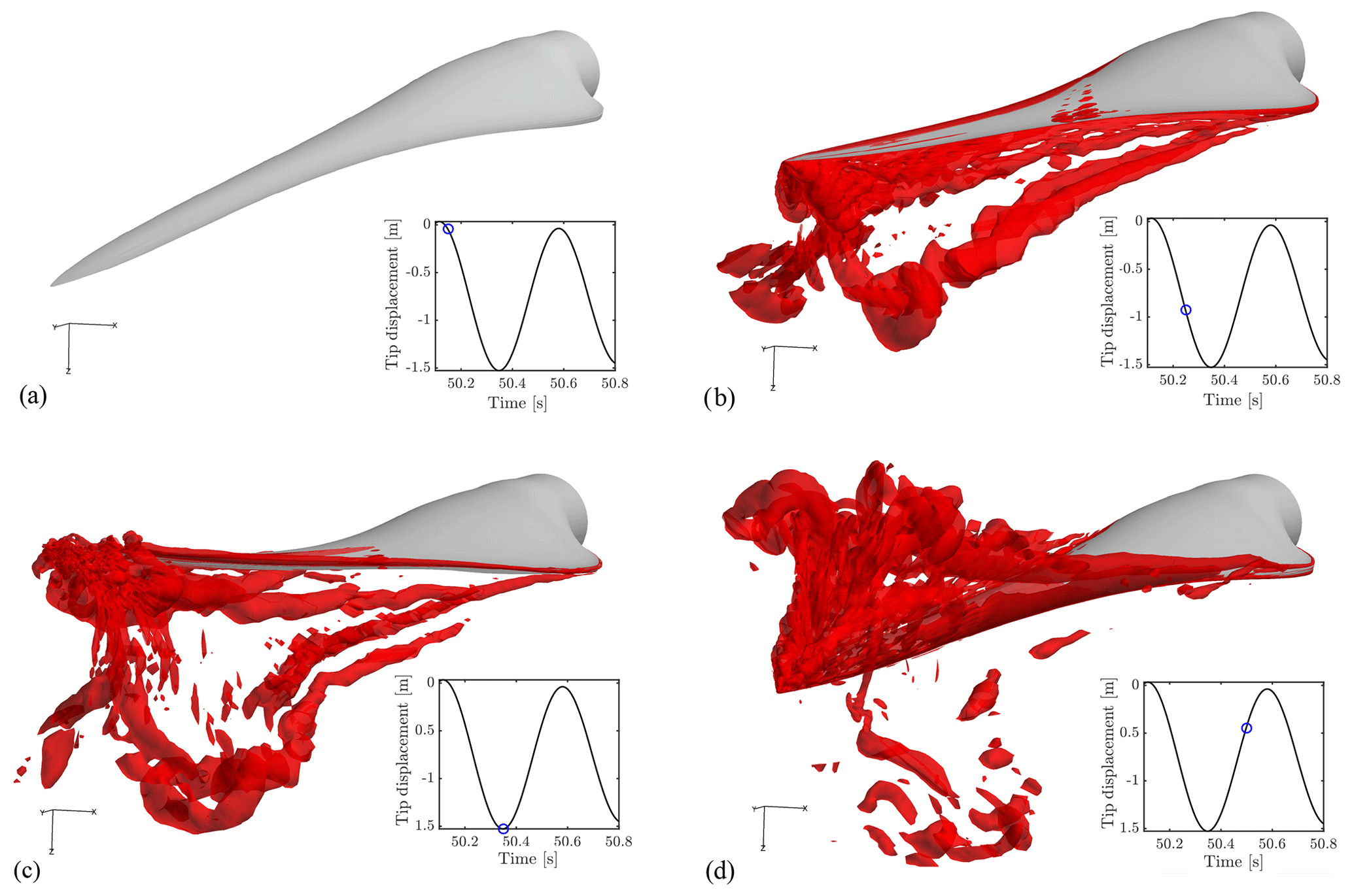
Figure 7 Isobars of the Q criterion during oscillation in the confined configuration. Q_crit=500. Graphs show the position of the blade tip for each figure.

As seen in Fig. 7b, vortices are created and shed from the blade as the blade is released, and at the turning point (Fig. 7c) many vortices are present in the wake. The blade travels through the vortices (Fig. 7d) and creates a new wake of vortices.

3.2 FSI validation

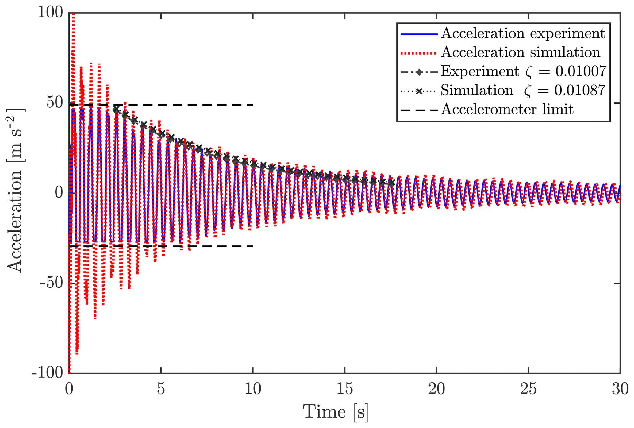
From the experimental test, the acceleration at 12.8 m was measured with an accelerometer. This measured acceleration will in the following be used for comparison between simulations and the experiment.

As seen in Fig. 8, the measurements and the FSI-CFD results compare well. For all cases, a decay factor ζ was estimated for the first part of the free oscillation. This decay factor does not consist of the aerodynamic damping alone but is rather a way of comparing the effective total damping between experiments and simulations. The aerodynamic damping will change during the oscillations, as it is dependent on the squared velocity and the drag coefficient, which might not be constant either. The decay factors are seen to be very comparable with a difference of 7 %. Note that these decays are approximated for a limited number of cycles only, using the logarithmic decrement. The same number of cycles is used from both the experimental and simulation results.

Figure 8 Acceleration measured in the experiment and simulated using FSI-CFD at 12.8 m.

Looking at the power spectral density (PSD) of the test and simulation acceleration signals, it is also evident that the three mode frequencies are found at around 2.15, 4.6 and 7.0 Hz for both tests and simulations.

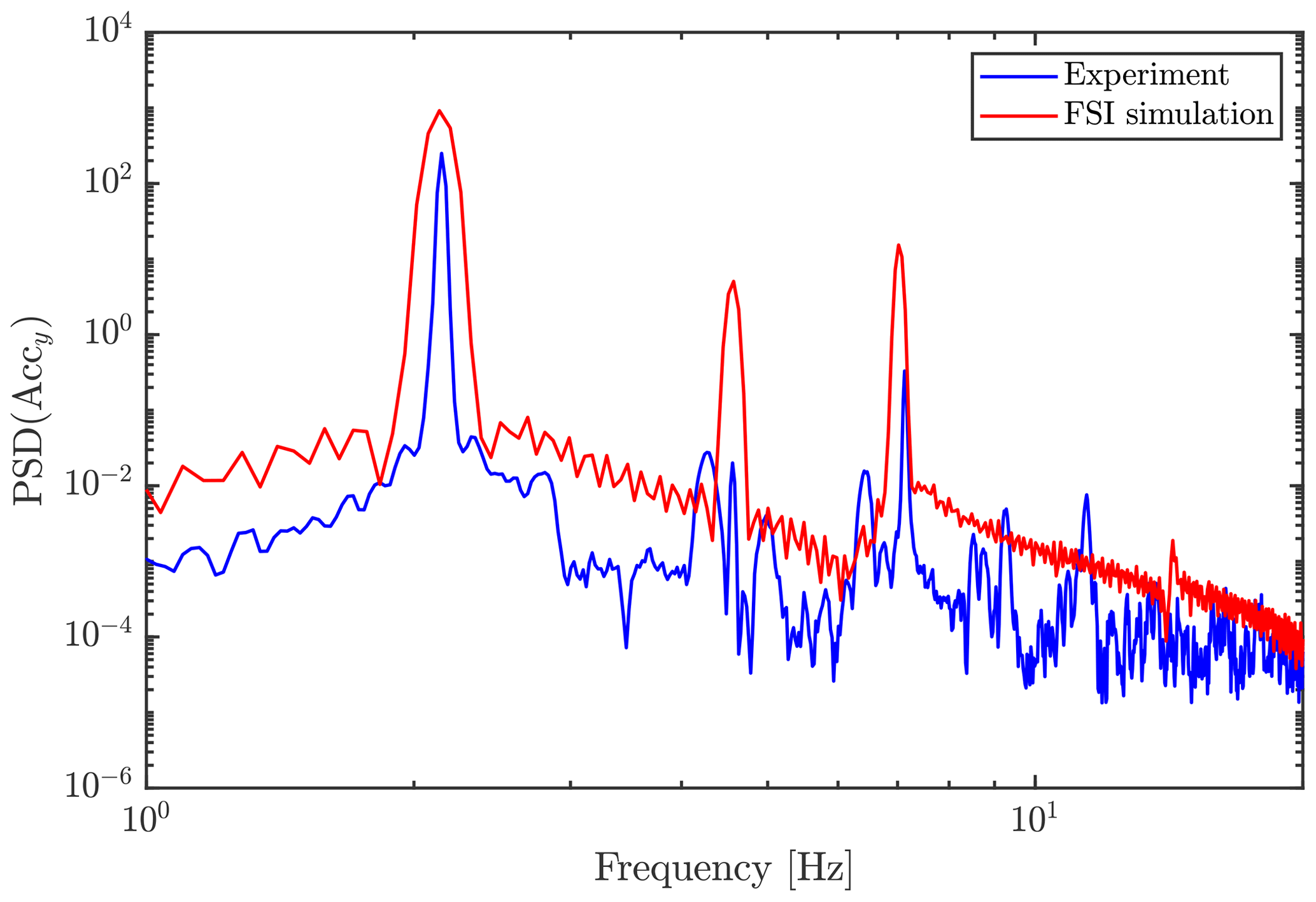
Figure 9 Power spectral density (using Welsh estimate) of acceleration signals of the experiment and simulation.

Figure 10 Strain calculated and measured at the suction side (a) and pressure side (b) of the blade at 63 % of the length of the blade.

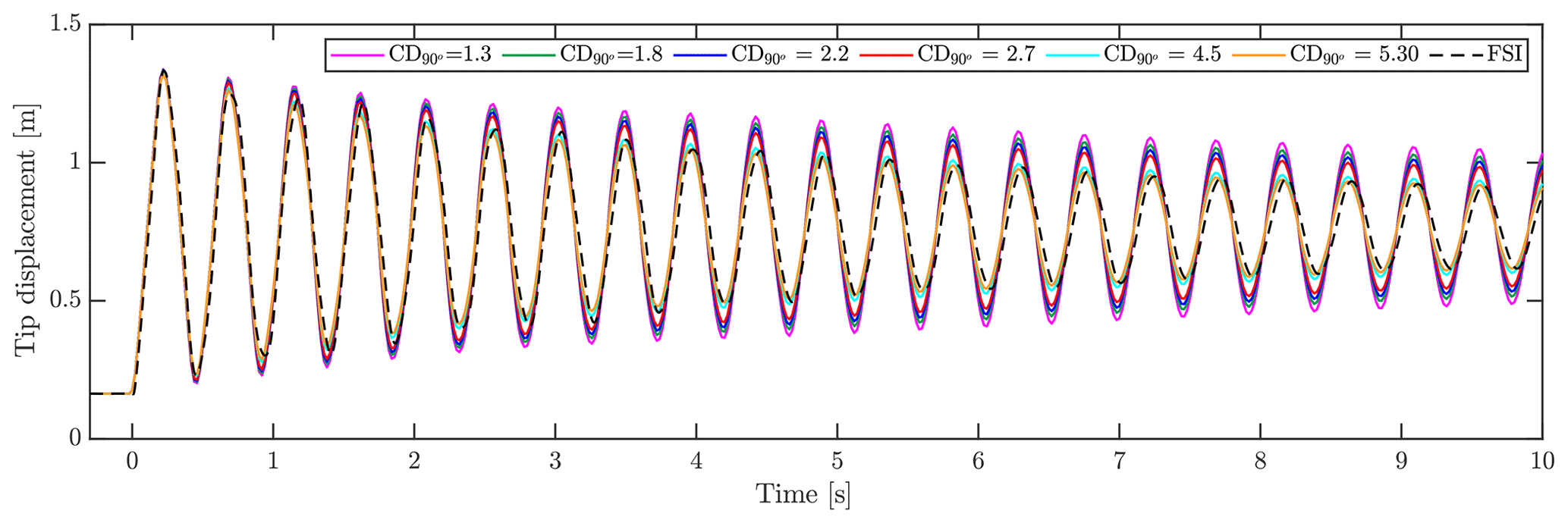
Figure 11 Tip displacement using BET aerodynamics with different drag coefficients compared with FSI results. All simulations have an initial tip displacement of 600 mm.

From the beam moments, found through simulations, the strains were found for the locations of the strain gauges used in the experiment, using Eq. (2), omitting any axial forces and any effects related to the stiffness matrix cross-talk term EI_xy.

$$\begin{array}{}\text{(2)}& \mathit{ϵ}={\displaystyle \frac{M_x}{E{I}_x}}y+{\displaystyle \frac{M_y}{E{I}_y}}x\end{array}$$

Strain gauge calibration was carried out beforehand by means of a static blade pull. As seen in Fig. 10, the calculated and measured strain agree well but have calculations overshooting the strain, especially at the suction side of the blade. This overshoot happens before release as well, where CFD has no influence, thus the reason must be a mismatch between the structural model and the tested setup or the coordinates of the strain gauges. A cumulative uncertainty is present, as Young's modulus (E), moments of inertia (I_x and I_y), strain gauge positions (x and y) and moments (M_x and M_y) will all have discrepancies between the model and the real blade. As a quantitative example, the relative difference in strain amplitude between experiment and simulations of the peaks at ≈4.68 s yields overshoots of 30.3 % at suction side and 6.0 % at the pressure side.

3.3 Drag coefficient calibration

As mentioned earlier, the standard practice for using the BET quasi-steady aerodynamics for simulations of tests is to increase the drag coefficient C_D to consider the additional drag resistance in test cases compared to normal flow conditions. In the following, FSI-BET results are shown for multiple different drag coefficients and compared with the FSI-CFD. The case of 600 mm initial tip displacement is used throughout. The calibration of drag in the present case was done by simply shifting the entire drag curve by constants, such that C_D at 90^∘ angle of attack reaches a chosen value. In this case, with an almost pure translatory motion, the angle of attack will be close to ±90^∘ at all times. For other tests with motion in different directions, such as a bi-axial fatigue test, the pure shift of C_D might not be an ideal method, as one could imagine that the added resistance due to vortices will be quite limited for small angles of attack. The original drag coefficient of the profile at 90^∘, $C_{\mathrm{D},\mathrm{90}{}^{\circ }}$, found for operational conditions through 3D CFD is 1.3. This $C_{\mathrm{D},\mathrm{90}{}^{\circ }}$ is lower than the range stated by Montgomerie (1996), due to 3D effects included in the simulations, thereby reducing the drag. Drag coefficients known to be used by industry and research groups of 1.8, 2.2, 2.7, 4.5 and 5.30 were applied to the FSI-BET simulations. As seen in Fig. 11, showing the tip displacement of the blade, the drag coefficients reach 4.5–5.30 before achieving similar damping as the FSI-CFD simulation. This value fits well with the drag coefficients stated by Greaves (2013) for the calibration with 2D CFD simulations of 5.30 and 4.45 for 1 and 2 m amplitudes, albeit on another profile.

Taking a close look at the first few oscillations of the FSI-BET simulations shown in Fig. 11, the best fitting drag coefficient is around 2.7, while after a few seconds the simulations using a C_D of 5.30 fit much better, indicating a varying drag coefficient through the vibration. Peaks at 1.15 s yield a 1.2 % overshoot for C_D=2.7 and −2.2 % for C_D=5.30. At 7.2 s, however, C_D=2.70 results in a 8.0 % overshoot, while C_D=5.30 overshoots with only 0.6 %. In this way, C_D=5.30 represents the total simulation better when using a constant drag coefficient, which is also visible in Fig. 11.

Inspecting the effective drag coefficients of the FSI-CFD simulations with varying initial deflections, Fig. 12 displays the node displacement of the 12.8 m node for the first 15 s after release, along with the corresponding force coefficient in the flapwise direction.

Figure 12 Oscillation of the node at 12.8 m and the corresponding force coefficient.

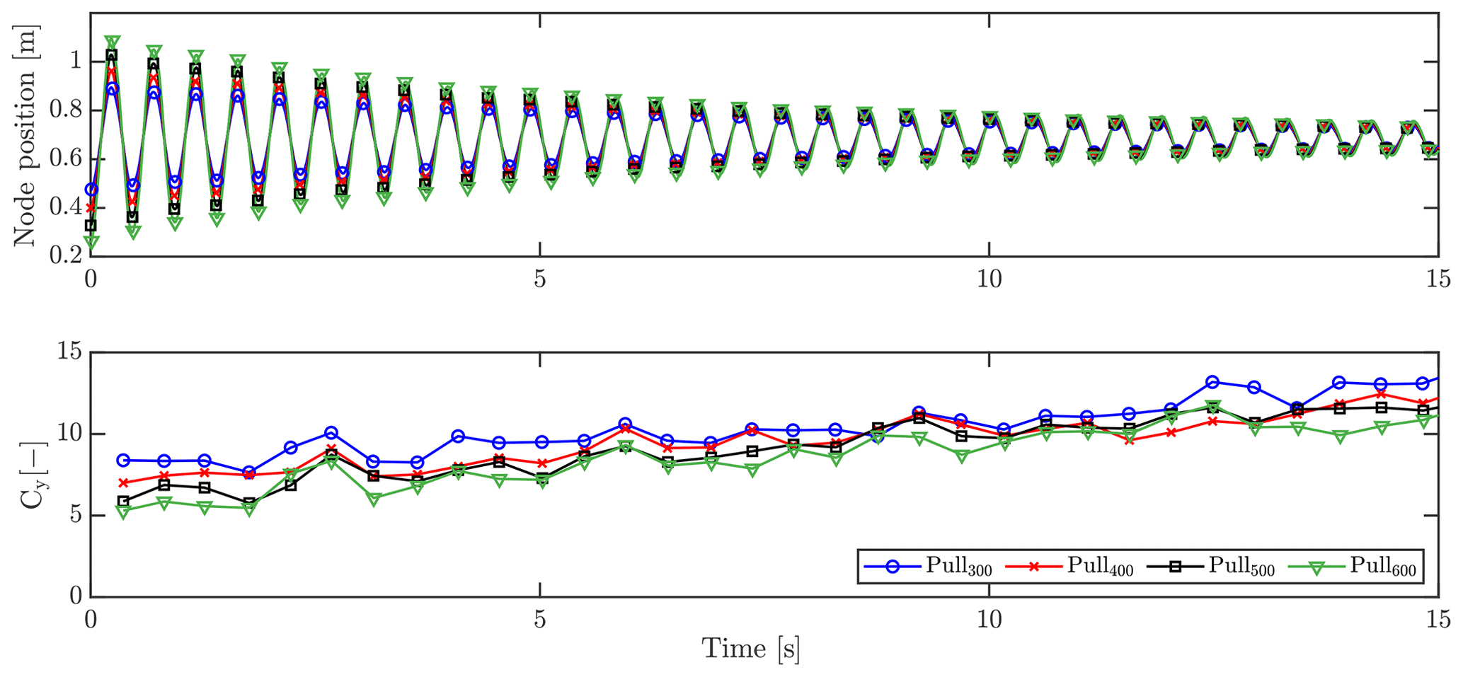
It has been shown that the force coefficient increases during the vibration as the amplitude decreases. This relationship is also seen from the initial force coefficients of 5.3, 5.9, 7.0 and 8.4, respectively, for 600, 500, 400 and 300 mm initial tip displacements. It is not possible to conclude anything about the relationship between amplitude and force coefficients with the chosen number of cases, but it is clear that future investigations are relevant. As has been shown, the initial force coefficient fits well with the aforementioned calibrated coefficient of 5.3 using the BET simulations of the 600 mm pull (Fig. 11). The reason for the calibrated drag coefficient not needing to increase during the simulation to fit the FSI-CFD results is due to the fact that the aerodynamic force is dependent on the squared velocity. This means that for large amplitudes, i.e., large velocities, the drag force will dominate, while decreasing in impact as the amplitude decreases.

Based on this investigation, drag coefficient calibration of BET-based fatigue test simulations should follow the actual amplitude of the blade during the test. Taking into account the different amplitudes along the blade by having multiple look-up tables for force coefficients depending on amplitude could resolve this. This would, however, require some development on the existing code. The chord length of the blade might also affect this dependency, but this has not been studied further here.

3.4 Influence of increased drag

To assess the impact of the increased drag on the fatigue test load simulations, a preliminary study was made. Here, BET-based simulations were conducted to obtain moment distributions along the blade for different drag cases. The simulation results were compared to the target moment distributions of the specific fatigue test. As a case study, a flapwise fatigue test for $N=\mathrm{2}\times {\mathrm{10}}^{\mathrm{6}}$ cycles was considered. The blade was modeled as described in Sect. 2.4. A set of tuning masses was installed on the blade, whereas the force excitation was applied by means of a translating mass exciter. Tuning masses were modeled as concentrated masses and located at specific beam nodes. The exciter was modeled as a predefined mass translating on a linear path at the flapwise resonance eigenfrequency, which was evaluated for the blade system including tuning masses and excitation mass. The location and magnitude of the tuning masses and the excitation parameters were determined beforehand. The test target loads M_tgt were also provided as an input based on the blade lifetime fatigue calculations carried out in Galinos (2017). A simulation time T_sim=100 s was adopted for all the test cases, excluding the initial transient loading which was disregarded. The rainflow counting algorithm developed in Nieslony (2010) was implemented in a MATLAB script used to evaluate the achieved test bending moment. Equation (3) was used to determine the so-called 1Hz equivalent load, where i indicates the ith bin, n_i the number of counted cycles for the ith bin, M_i the bending moment amplitude for ith bin, m the Stress-Cycle (S-N) curve slope parameter and N_1 Hz the number of cycles of a 1 Hz signal in a time interval equal to T_sim. The S-N curve slope parameter was chosen equal to 12, which is typical for blades manufactured in glass-fiber-reinforced composite material, as the one used in this study. The test load was subsequently calculated by Eq. (4), which accounts for the flapwise resonance testing frequency f_flap.

$$\begin{array}{}\text{(3)}& {\displaystyle }& {\displaystyle }{M}_{\mathrm{1}\mathrm{Hz}}={\left({\displaystyle \frac{\sum _i{n}_i{M}_i^m}{N_{\mathrm{1}\mathrm{Hz}}}}\right)}^{\frac{\mathrm{1}}{m}}\text{(4)}& {\displaystyle }& {\displaystyle }{M}_{\mathrm{test}}={\left({\displaystyle \frac{M_{\mathrm{1}\mathrm{Hz}}^m}{f_{\mathrm{flap}}}}\right)}^{\frac{\mathrm{1}}{m}}\end{array}$$

Figure 13 (a) Variation in the achieved flapwise test bending moment along the blade with respect to the target load for different drag coefficients and (b) variation in the test bending moment normalized against the root bending moment as a function of the drag coefficient for different blade span locations.

Table 1 describes the test setup adopted during the presented set of simulations, in which the only varied parameter was the drag coefficient. The excitation parameters, i.e., the excitation mass longitudinal position (z_e), the excitation mass magnitude (m_e) and the excitation mass oscillation amplitude (s_e), were chosen to achieve a relative test bending moment of approx. 100 % in the blade portion and between 20 % and 80 % of the blade span for the test setup, with a maximum value of C_D equal to 1.8 for an angle of attack of 90^∘. The excitation parameters were then kept constant for varying C_D curves with maximum value in the range between 1.3 and 5.0, as done in Sect. 3.3, where 1.8 was taken as baseline since 1.3 is expected to underestimate the blade loading.

Table 1 Flapwise test setup with indication of location z_t and magnitude m_t of the tuning masses, location z_e, mass magnitude m_e and stroke s_e of the exciter, and excitation frequency f_flap.

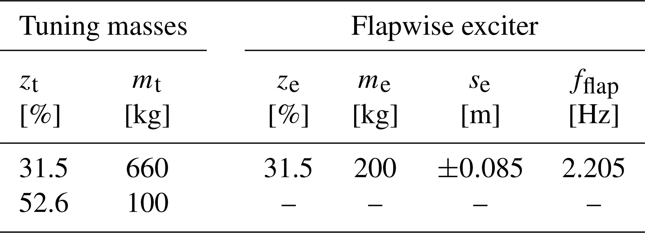
Figure 13 shows the variation in the achieved test bending moments along the blade span for a varying C_D in the defined range. In Fig. 13a it can be noticed how the achieved test load decreases with increasing C_D. The load reduction is highlighted in Fig. 13b by representing the variation in the achieved bending moment M_norm, normalized with respect to the baseline case (C_D=1.8), as a function of the drag coefficient. It can be concluded that the decrease in achieved test load follows the same trend for different locations along the blade span. Moreover, it was observed that the achieved load variation is nonlinear and presents a slope which appears to be decreasing for increasing drag coefficients.

3.5 Confinement influence

As described in Sect. 2.3.1, different configurations were treated to study the possible influence of the confined space around the tested blade. The same four pull distances were tested with and without confinement, and the resulting tip displacements and aerodynamic forces were compared. As shown in Fig. 14, the confined and unconfined setup yields very similar results for aerodynamic forces and results in essentially identical displacements, indicating that the confinement has no effect in the present setup.

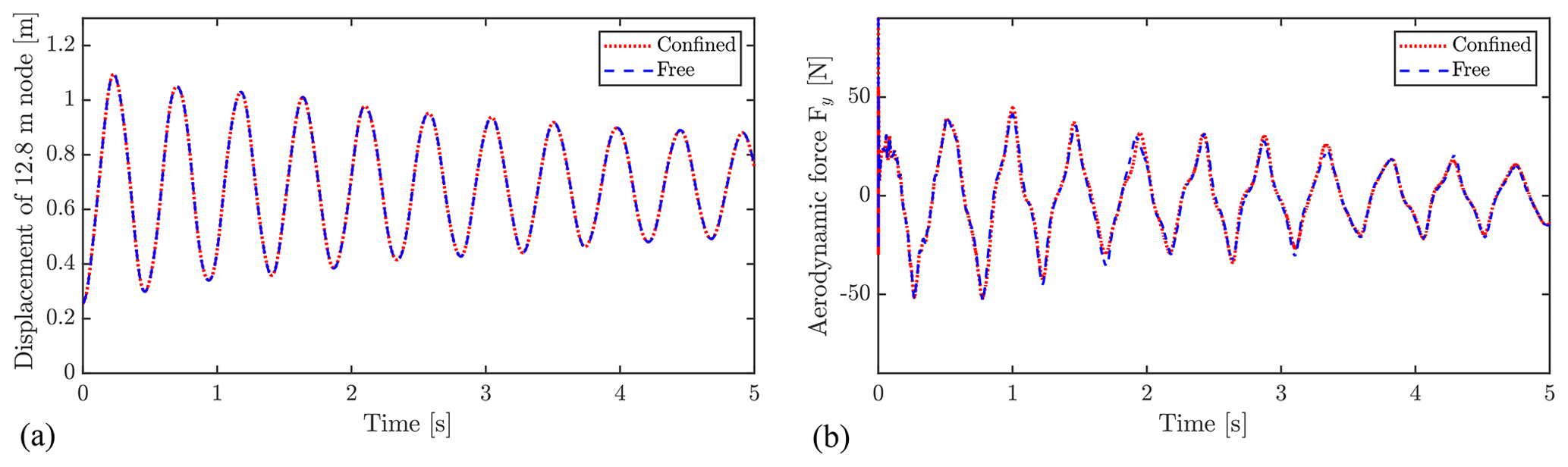
Figure 14 Confinement effect on displacement (a) and aerodynamic forcing (b) on the node at 12.8 m.

Figure 15 depicts, respectively, the pressure and velocity field around the blade at the time of the blade passing its equilibrium position, i.e., approximately at maximum velocity. It is evident that the gradients of pressure and velocity near the floor and walls are small, which supports that the effect of the confinement is negligible. As the blade velocity will decrease when moving closer to the floor, the blockage effect will decrease as well. However, it is also shown that a large zone of high pressure, is created beneath the blade, which in cases of longer blades with larger chords, might grow sufficiently to interact with the floor. In large test facilities, blades that are 5–7 times longer than the design studied in the present work are tested. The ratios between blade length and wall and floor distance for these cases will be different than the one studied here. In the minds of the authors, the possible effect should be tested using one of these blades with a similar FSI setup before drawing general conclusions about the effect of confinement.

Figure 15 Confined configuration: (a) pressure field and (b) vertical (z) velocity field.

4 Conclusions and future studies

This study has been conducted to investigate the special aerodynamic circumstances present during full-scale structural experiments in blade test facilities, being high drag forces during flapwise vibration and confinement of air in the test facility. These phenomena are important for, e.g, fatigue tests, where millions of vibration cycles are forced using exciters, requiring a large amount of energy.

Three-dimensional high-fidelity fluid–structure interaction simulations (FSI-CFD) of pull–release tests on a ≈14m wind turbine blade have been conducted and analyzed. Results are compared to experimental results to validate the simulations, and in general a good agreement is seen. Accelerations measured on the blade during the experiment and simulated through the FSI-CFD show similar damping, quantified by a decay factor ζ, with a relative difference of 7 % for the tested case of 600 mm initial tip displacements. Measured strains are compared to those calculated from resulting moments of FSI-CFD. Here the pressure side strains are predicted well, whereas overshoots are seen in the suction side strains, probably due to discrepancies between structural model and actual blade.

Simulation results are used to study the flow field around the oscillating blade, and investigate the impact of the blade moving through its own whirling wake along with the confined conditions of a test facility. Through visual inspection of the calculated flow field, it is evident that large vortices are created behind the moving blade, which the blade has to travel back through when changing direction. This causes the effective drag force coefficients on the blade to significantly exceed those seen during normal operation. In the specific case of 600 mm initial tip displacement, a drag coefficient for the 90^∘ angle of attack ($C_{\mathrm{D},\mathrm{90}{}^{\circ }}$) of BET-based FSI needs to be increased to 5.3 from the original 1.3, in order to fit FSI simulations, using CFD aerodynamics. However, it is found that the drag coefficient varies with amplitude as to why, one specific drag coefficient will not cover all cases.

A single-axial flapwise fatigue test simulation was used as case study to evaluate the impact of the C_D choice on the test load calculation. For a constant test load setup, the C_D curves were varied in a range of peak values between 1.3 to 5.3 for an angle of attack of 90^∘, which provoked a nonlinear decrease in the achieved test load of approx. 25 % with respect to the target loads. This proves that the correct choice of the C_D coefficient is crucial for the validation of aeroelastic test simulations against experimental results.

An interesting topic to study further is the dependency between the increase in drag coefficient and the ratio between oscillation amplitude and chord width. For small amplitudes, the blade passes through the wakes all the time, while large amplitudes might create enough distance to the shed wakes to only be affected right at the turn of direction. This could lead to the drag-to-amplitude dependency only being present at low amplitudes, as seen for flat plates in Woolam (1968). There might also be a dependence on the oscillation frequency, which sets the velocity of the blade; however, this was not the case for flat plates in Woolam (1968).

A mapping of force coefficients depending on motion could be added to the existing force coefficient tables, to conduct more accurate BET-based simulations of fatigue tests and possibly assist in choosing methods for fatigue testing to reduce the energy demand of the test.

The role of confinement due to the floor, walls and ceiling in the test facility is analyzed by using and comparing FSI-CFD simulation results with confined and unconfined setups. No impact is seen when comparing the results of the confined and unconfined setup, showing that confinement effects are negligible in the present case. A future study of the same effect on longer blades would be beneficial, as the ratio between blade-to-floor distance and blade length and chord width will change significantly.

A natural continuation to this work would also be to simulate actual fatigue tests, with both uniaxial and biaxial motion. A biaxial motion could possibly reduce the air resistance, as the blade would not move directly back through its own wake. The wake itself could also differ significantly using other motion patterns, making this an interesting study.

Appendix A: Sensitivity analysis – CFD

The following serves as a continuation of Sect. 2.3.1 and shows results of the sensitivity studies made concerning grid refinement, time steps and turbulence models. To simplify the sensitivity study, a one-way coupled FSI-CFD study was conducted using imposed motions. Instead of HAWC2-defined motions, an analytic polynomial expression of the vertical motion was applied, which resembles the case of 600 mm tip displacement to a satisfying degree. The frequency, amplitude and damping were calibrated to fit the initial results of the FSI-CFD results; however, the displacement due to gravity was not included. For practical reasons, instead of a release from the deformed state, the motion started from the initial position of the blade like a sinusoidal function.

The analytical expression used for the blade motion is as follows:

$$\begin{array}{}\text{(A1)}& \mathrm{Disp}=x^{\mathrm{2}}\cdot A\cdot \sin (\mathrm{2}\mathit{\pi }\cdot f\cdot t)\cdot e^{-\mathit{\zeta }\cdot f\cdot \mathit{\pi }\cdot t},\end{array}$$

where x is the coordinate along the blade, A is a constant, f is the motion frequency, t is time and finally ζ is a damping ratio. To fit the FSI-CFD results, the following values were used: A=0.0028, f=2.15 Hz and ζ=0.025. The tip displacement of the analytical expression is shown in Fig. A1, together with the FSI-CFD results, which are shifted upwards to omit the gravity displacement and a quarter period to the right. As seen here, the tip displacements agree well, justifying the use of the prescribed motion for sensitivity studies.

Comparison between tests is done by comparing amplitudes at two peaks, P₁ at ≈0.65 s and P₂ at ≈2.96 s, along with the damping ratio calculated using the logarithmic decrement between the points. Baseline tests are marked with “^*”.

A1 Grid sensitivity

To study the sensitivity of grid refinement, four versions of the grid were tested. All grids consisted of 158 blocks but using a different number of cells per block, i.e., 8³, 16³, 32³, 64³, where 32³ is the grid (level 1) used when creating the setup. Time steps were adjusted accordingly to obtain identical CFL numbers using $\mathrm{\Delta }t=\mathrm{5}\times {\mathrm{10}}^{-\mathrm{4}}$ s for the baseline and halving the time step when doubling the refinement and vice versa. As seen in Fig. A2 and Table A1, the finest setup and the baseline, level 0 and level 1, respectively, result in very similar results with only small differences of −0.41 % at P₁, −3.54 % at P₂ and 2.52 % for ζ.

A2 Time step sensitivity

Three different time steps, $\mathrm{5}\times {\mathrm{10}}^{-\mathrm{3}}$, $\mathrm{1}\times {\mathrm{10}}^{-\mathrm{3}}$ and $\mathrm{5}\times {\mathrm{10}}^{-\mathrm{4}}$ s, were tested to find an optimum for the FSI-CFD simulations. The results are depicted in Fig. A3 and Table A2, and it is shown that there is practically no difference between $\mathrm{1}\times {\mathrm{10}}^{-\mathrm{3}}$ and $\mathrm{5}\times {\mathrm{10}}^{-\mathrm{4}}$ s, with errors of 1.69 % at P₁, −1.56 % at P₂ and 2.50 % for ζ.

A3 Turbulence model sensitivity

Turbulence models were initially meant to be included, but it quickly revealed that the special case of no flow in the domain caused these models to become unstable. For this reason different methods were compared, i.e., k−ω SST, DES k−ω SST and finally without any turbulence model enabled, such that a DNS-like simulation is run.

In the presented case, the k−ω model crashed during the first cycle, while the DES k−ω SST seemed more stable but with sudden jumps until finally crashing. Many attempts were conducted using varying schemes, inlet turbulence parameters and time steps (among others) to create a stable run using turbulence models, but none were successful. As seen in Fig. A4 and Table A3, the three models result in similar forces on the blade, with differences of −4.51 % at P₁, 3.32 % at P₂ and −5.7 % for ζ, between DNS and DES.

A4 Conclusion of sensitivity analysis

From the presented sensitivity studies of grid levels, time steps and turbulence models used, the following setup was chosen: for grid refinement the original grid (level 1) was deemed sufficiently fine for the FSI-CFD simulations, taking into account the computational efforts necessary to use the finer grid.

Due to stability issues, it was chosen not to use any turbulence model and use the DNS like approach. It must be emphasized, however, that the grid was not fine enough to resolve all turbulent scales, as required for a proper DNS simulation. However, the scales of the important vortices were resolved sufficiently well, and the errors compared to the DES k−ω SST model were small.

For the time step, it was chosen to use $\mathrm{5}\times {\mathrm{10}}^{-\mathrm{4}}$ s for the FSI-CFD simulations throughout, despite $\mathrm{1}\times {\mathrm{10}}^{-\mathrm{3}}$ s resulting in small errors only. This choice was made to compensate for some of the error seen when using no turbulence models.

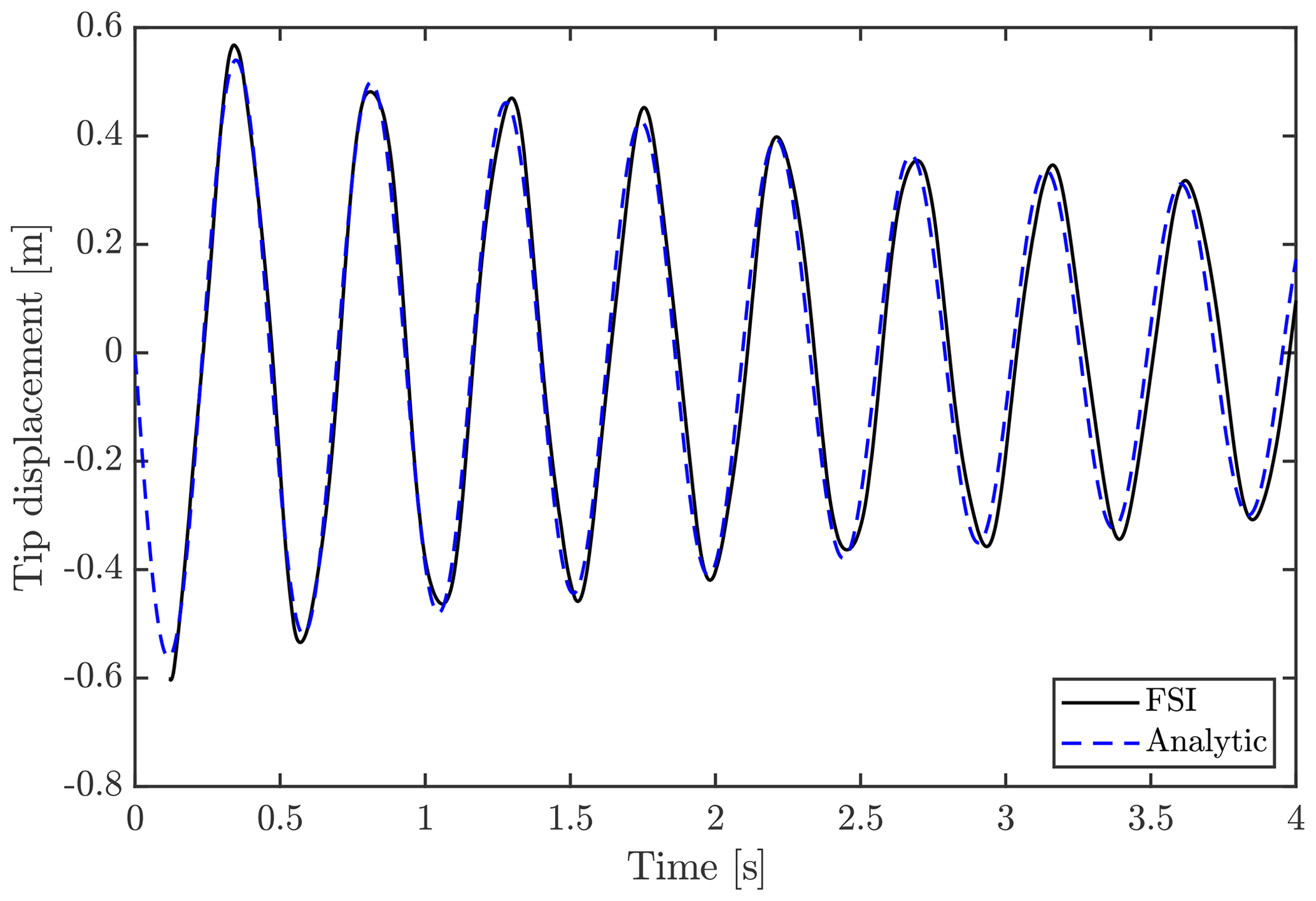
Figure A1 Tip displacement using analytical expression, compared to result from FSI-CFD with 600 mm initial tip displacement. Note that the FSI-CFD result is shifted with the equilibrium position, due to gravity, and a quarter period to the right.

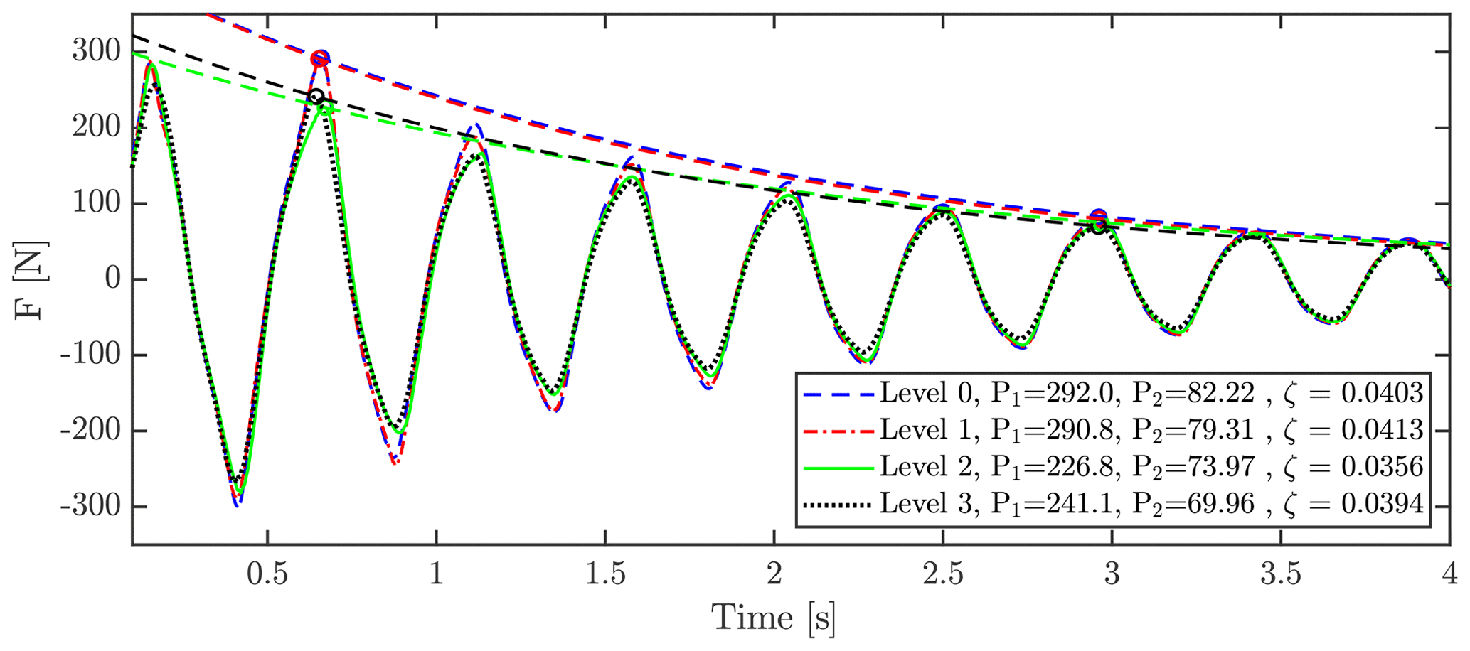
Figure A2 Grid sensitivity study using a different number of cells per block. A total of 158 blocks was used. Level 0 was $\mathrm{64}\times \mathrm{64}\times \mathrm{64}$ per block, i.e., 41 418 752 cells in total. Level 1 was $\mathrm{32}\times \mathrm{32}\times \mathrm{32}$ per block, i.e., 5 177 344 cells in total. Level 2 was $\mathrm{16}\times \mathrm{16}\times \mathrm{16}$ per block , i.e., 647 168 cells in total. Level 3 was $\mathrm{8}\times \mathrm{8}\times \mathrm{8}$ per block,i.e, 80 896 cells in total.

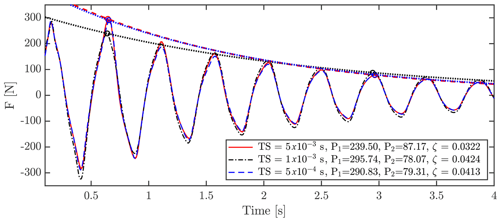
Figure A3 Sum of aerodynamic forces on the blade during vibration using time steps of $\mathrm{5}\times {\mathrm{10}}^{-\mathrm{3}}$, $\mathrm{1}\times {\mathrm{10}}^{-\mathrm{3}}$ and $\mathrm{5}\times {\mathrm{10}}^{-\mathrm{4}}$.

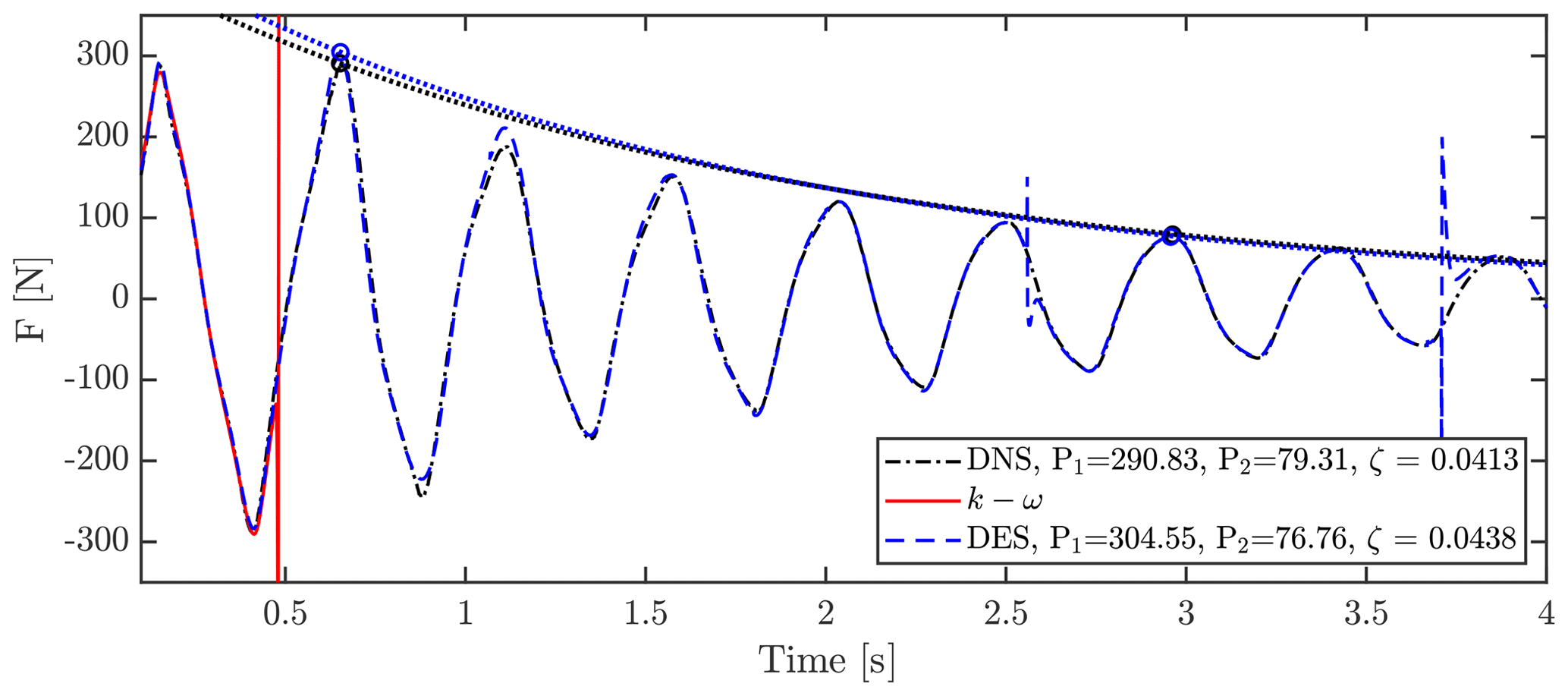
Figure A4 Sum of aerodynamic forces on the blade during vibration using no turbulence model (pseudo-DNS), k−ω SST and DES k−ω SST.

Table A1 Comparison of peaks and damping ratios for different grid levels.

^* Denotes the baseline case used to calculate relative errors.

Table A2 Comparison of peaks and damping ratios for different time steps.

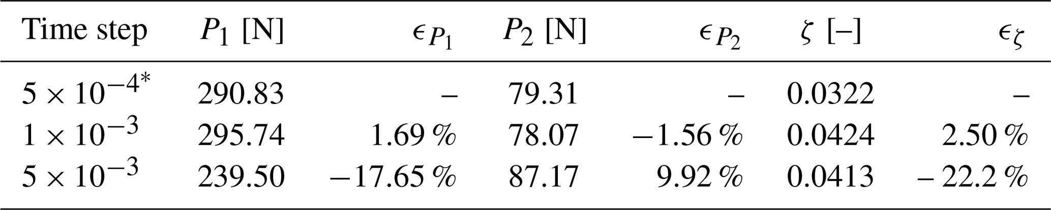
^* Denotes the baseline case used to calculate relative errors.

Table A3 Comparison of peaks and damping ratios for different turbulence models.

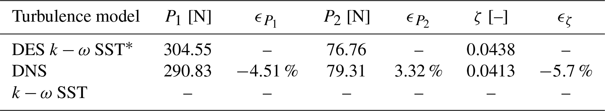
^* Denotes the baseline case used to calculate relative errors.

Appendix B: Sensitivity study – structural damping

As mentioned in Sect. 2.4, the structural damping of the model was tuned beforehand to 1 % logarithmic decrement using Rayleigh damping in HAWC2. This value is a choice that is conservatively based on the findings of Post (2016). However, it is difficult to assess the exact value of structural damping through experimental tests, as the aerodynamic damping cannot be excluded entirely. To investigate the impact of the structural damping, a small study was done using HAWC2-based simulations with different structural damping parameters of 0 %, 1 %, 2 % and 3 % logarithmic decrement. The 90^∘ aerodynamic drag coefficient was set equal to 5.3, as was found to be suitable for the setup in the FSI study. A case without aerodynamic forces and 1 % logarithmic decrement structural damping is added to clarify the different impact of aerodynamic and structural damping. The tip displacement of the blade using the different damping coefficients is depicted in Fig. B1. It has been shown that the difference in structural damping from 1 %, 2 % and 3 % logarithmic decrement only result in minor differences in the tip displacement result. It is also clear that the aerodynamic damping added by introducing a drag coefficient of 5.3 dominates the total damping.

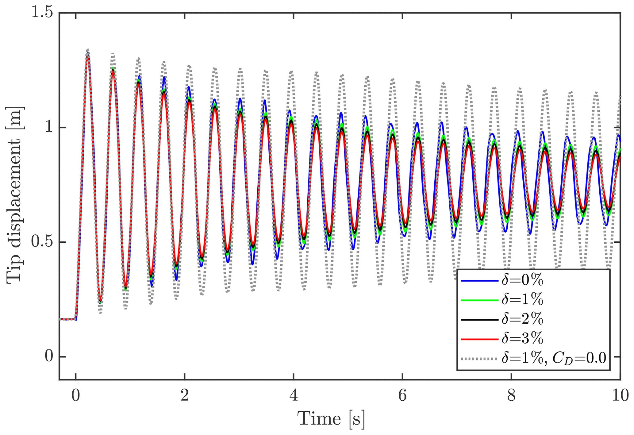
Figure B1 Tip displacement using 0 %, 1 %, 2 % and 3 % logarithmic decrement structural damping and CD₉₀=5.3. A simulation without aerodynamic drag (CD₉₀=0.0) and 1 % logarithmic decrement structural damping has been added for comparison.