the Creative Commons Attribution 4.0 License.
the Creative Commons Attribution 4.0 License.
 | 01 Nov 2021
Experimental analysis of radially resolved dynamic inflow effects due to pitch steps
David Onnen
Gerard Schepers
Martin Kühn
The dynamic inflow effect denotes the unsteady aerodynamic response to fast changes in rotor loading due to a gradual adaption of the wake. This does lead to load overshoots. The objective of the paper was to increase the understanding of that effect based on pitch step experiments on a 1.8 m diameter model wind turbine, which are performed in the large open jet wind tunnel of ForWind – University of Oldenburg. The flow in the rotor plane is measured with a 2D laser Doppler anemometer, and the dynamic wake induction factor transients in axial and tangential direction are extracted. Further, integral load measurements with strain gauges and hot-wire measurements in the near and close far wake are performed. The results show a clear gradual decay of the axial induction factors after a pitch step, giving the first direct experimental evidence of dynamic inflow due to pitch steps. Two engineering models are fitted to the induction factor transients to further investigate the relevant time constants of the dynamic inflow process. The radial dependency of the axial induction time constants as well as the dependency on the pitch direction is discussed. It is confirmed that the nature of the dynamic inflow decay is better described by two rather than only one time constant. The dynamic changes in wake radius are connected to the radial dependency of the axial induction transients. In conclusion, the comparative discussion of inductions, wake deployment and loads facilitate an improved physical understanding of the dynamic inflow process for wind turbines. Furthermore, these measurements provide a new detailed validation case for dynamic inflow models and other types of simulations.
- Article
(10509 KB) - Full-text XML
- BibTeX
- EndNote


Dynamic inflow describes the unsteady response of loads to fast changes in rotor loading, e.g. due to fast pitching of the rotor blades or gusts. This unsteady aerodynamic effect leads to load overshoots due to the inertia of the global flow field, as the axial wake induction in the rotor plane cannot change instantaneously but only gradually to a new equilibrium flow field.
In addition to the direct impact on the dynamic loading, van Engelen and Hooft (2004) emphasise the need to model these dynamic inflow effects for the pitch controller design to enhance the stability and thus reduce unnecessary fatigue loads with optimised pitching transients, especially near rated operation. The dynamic wake behaviour due to load changes is intrinsically considered in higher-fidelity approaches as computational fluid dynamics (CFD) and free vortex wake method (FVWM) simulations, thus modelling the dynamic inflow effect. However, engineering models are required to mimic this effect in blade element momentum (BEM) theory, which is commonly applied for aeroelastic simulations for the design and certification of wind turbines. Well-tuned engineering models help to avoid too conservative predictions of fatigue loads.
First extensive studies in the 1990s within the Joule I and II projects on the development of dynamic inflow models for wind turbines are described in Snel and Schepers (1995) and Schepers and Snel (1995). There the free field measurements of out-of-plane blade root bending moment and rotor shaft torque for pitch steps on the 2 MW Tjæreborg wind turbine, described in Øye (1991), are used for validation.
Later Schepers (2007) employed a one-time-constant model to analyse force transients. These are derived from pressure sensor arrays at five radial stations, after the pitch steps of the NREL (National Renewable Energy Laboratory) phase VI turbine with 10 m diameter (see Hand et al., 2001) in the NASA Ames wind tunnel. Forces for the pitch step to low load adapt faster to the new equilibrium than for the step to high load. They could not experimentally validate the strong radial dependency of the time constant, which they expect from cylindrical wake models. Sørensen and Madsen (2006) also investigated the same experiment and compared it to unsteady Reynolds-averaged Navier–Stokes (uRANS) CFD simulations. They suggest using a two-time-constant model to capture the dynamic inflow effect on the forces. The fast time constant represents the near-wake dynamics and decreases with radius, and the slow time constant represents the far-wake dynamics. Later Pirrung and Madsen (2018) investigated this experiment and uRANS CFD simulations again and compared them to a cylindrical wake model. Based on varying the wake length in the cylindrical wake model, they affirm that two different time constants best describe the dynamic inflow effect.
Within the Model EXperiment In controlled COnditions (MEXICO) framework, pitch steps are performed on a 4.5 m diameter model wind turbine, featuring pressure distribution measurements at five radial stations, as well as in high- and mid-fidelity simulations (Boorsma et al., 2018). They find that unsteady aerodynamic effects on the blade chord level, namely the Theodorsen effect, reduce the load overshoot. This effect can be modelled as a time lag on the angle of attack of the order of the ratio of relative wind to respective chord length. In contrast, the typical dynamic inflow time constant is of the order of the ratio of radius to free wind velocity and 2 orders of magnitude higher.
Yu et al. (2017) used an actuator disc with variable blockage in a wind tunnel to study the wake evolution after a change in thrust. We also presented a preliminary pitch step experiment in Berger and Kühn (2018), focusing on the integral turbine loads. The relevance of improved modelling of the dynamic inflow effect can be seen in the recent development of new dynamic inflow models by Yu et al. (2019), Madsen et al. (2020) and Ferreira et al. (2021).
Schepers and Schreck (2018) emphasise the value of experimental investigations of aerodynamic effects and also specifically the dynamic inflow effect to further improve and validate models. Higher-fidelity simulations depend on calibration and thus cannot solely fill this gap. Further, Schepers and Schreck (2018) outline the importance of radius-resolved aerodynamic measurements over integrated blade and rotor loads. No experimental investigation is available until now, where the wake induction is directly probed at various blade radii in the rotor plane.
The objective of this paper is to get deeper insights into the dynamic inflow effect for wind turbines due to pitch steps. The main novelty in this work is the dynamic induction measurement. The radial dependency and differences between the pitch directions are investigated using time constant analysis. Furthermore, the behaviour of the flow in the near and close far wake and integral loads are used to compare the differences between the pitch directions. These different measurements are contemplated together to allow for new insights into the dynamic inflow effect, test presumptions and validate findings of prior work.
In Sect. 2.1 the experiment is introduced. In Sect. 2.2 time constant models and the fitting approach are outlined. Lastly, in Sect. 2.3 the method for the load reconstruction based on the obtained wake inductions is outlined.
2.1 Experiment
In this subsection, all relevant information on the experiment is introduced, consisting of the setup, experimental matrix, wake induction derivation from measurements, ensemble averaging approach and correction models.
2.1.1 Setup
The experiments were performed in the large wind tunnel at ForWind – University of Oldenburg. It is a Göttingen-type wind tunnel that can be operated in an open jet or a closed test section configuration. The test section length measures 30 m, and the rectangular wind tunnel nozzle dimensions of 3 m by 3 m, as shown in Fig. 1 a. Wind velocities in the open jet configuration reach up to 32 m s−1. Kröger et al. (2018) provide detailed information about the wind tunnel and the optional active grid. No active grid was used in the measurement, and the turbulence intensity of the inflow was of the order of 0.3 %.
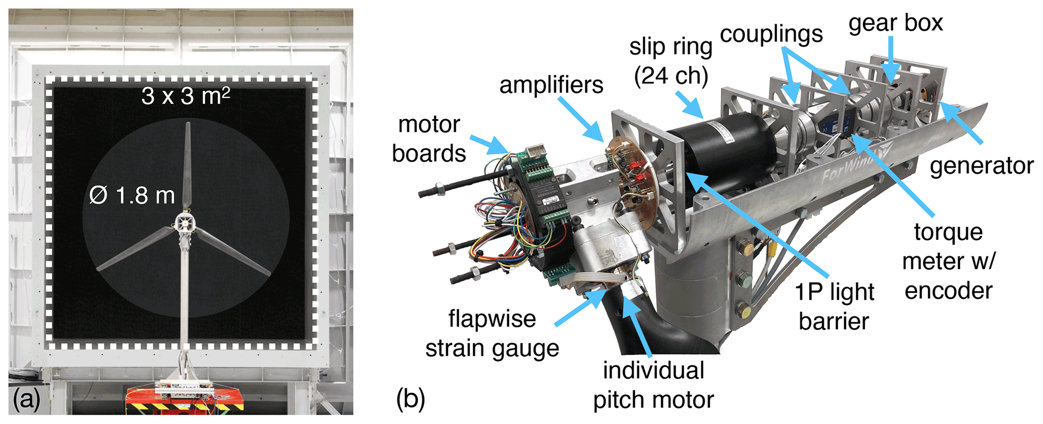
Figure 1(a) Wind tunnel nozzle and MoWiTO 1.8 with main dimensions. (b) MoWiTO 1.8 with open nacelle.
The utilised Model Wind Turbine Oldenburg has a diameter of 1.8 m (MoWiTO 1.8). The machine is an aerodynamically scaled version of the NREL 5 MW generic turbine (see Jonkman et al., 2009) with a length scaling factor of . The scaling approach was to maintain the design tip speed ratio, thrust and power characteristic, as well as non-dimensional lift and thus axial induction distribution for the operational range. Low Reynolds number airfoils were used. The rotor blades have a stiff carbon-fibre-based structure with the first eigenfrequency of 32 Hz and estimated maximum tip deflections of 0.01 m The scaling approach and turbine are described in detail in Berger et al. (2018). The blockage ratio of the turbine in the used open jet configuration wind tunnel is 0.28; however, Ryi et al. (2015) showed that blockage effects are negligible for such an open jet configuration.
The MoWiTO 1.8 nacelle is shown in Fig. 1b. The turbine features individual pitch motors, which are mounted in the root of each blade. The pitch motors are small DC motors with a three-stage planetary gearbox with a gear ratio of 159:1 and integrated encoders. They are mounted and pretensioned with springs to counteract gear backlashes and thus allow for setting precise pitch angles. Pitching speeds up to 100 Hz (1.75 rad s−1) can be achieved. The main shaft is supported by two roller bearings and connected by a coupling to a torque meter with an integrated encoder and through another coupling and one stage planetary gearbox to the generator. Flapwise blade root bending moments for each blade are measured by a full Wheatstone bridge strain gauge configuration on the metal adapter; the carbon-fibre blades are glued on. The power supply lines for the amplifiers and motor boards in the hub and their communication with the control hardware are channelled through a slip ring from the rotating hub to the stationary nacelle. Further, the thrust of the turbine is derived from a strain gauge measurement of the tower bottom bending in fore–aft direction, as outlined in Sect. 2.1.5. A National Instruments Compact Rio is used for control and data acquisition. Analogue data (e.g. strain gauges, external hot wires) are sampled at 5 kHz, and the control loop and pitch motor communication run at 100 Hz.
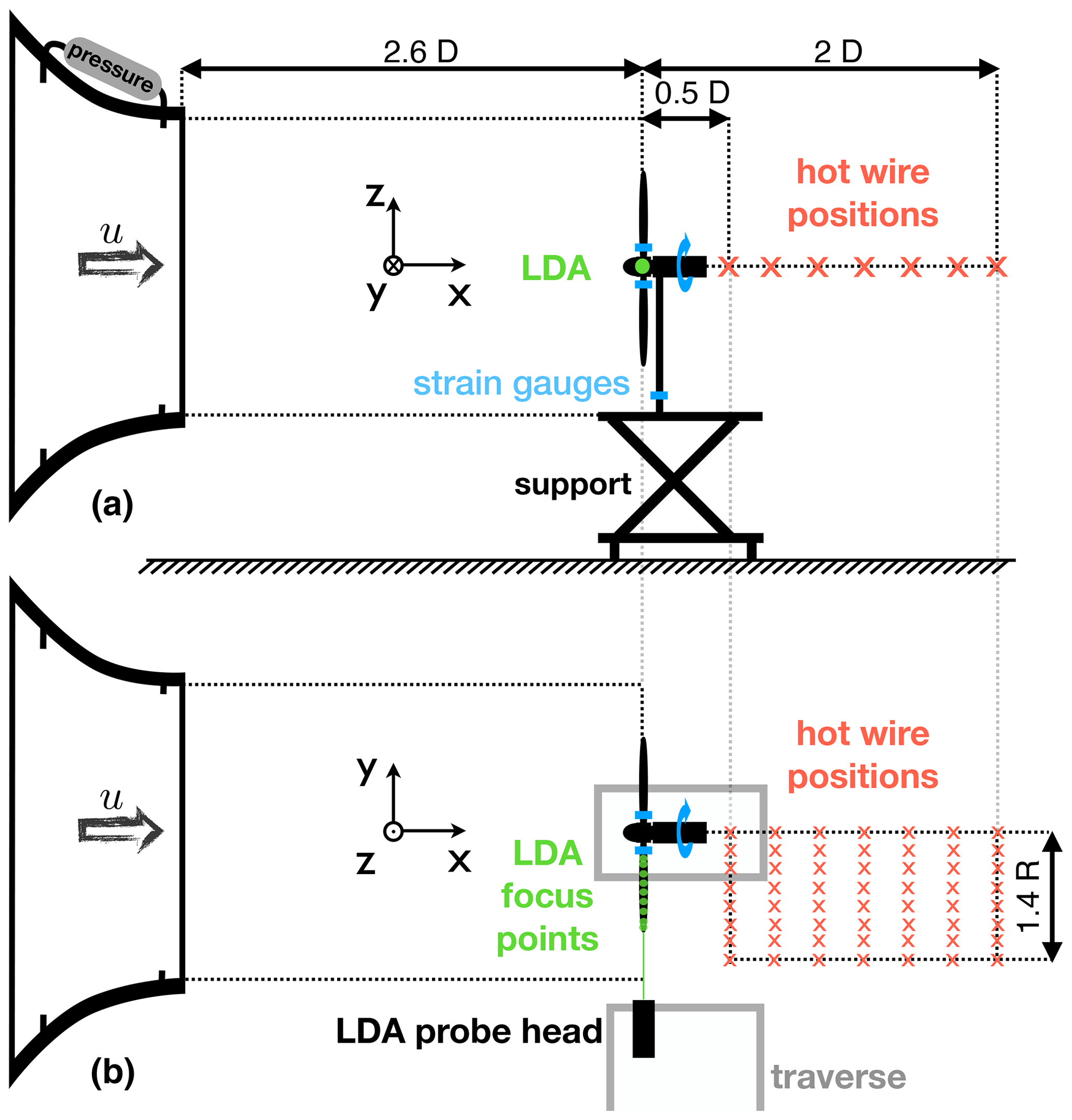
The setup of the MoWiTO 1.8 in the wind tunnel is sketched in Fig. 2a and b as a view from the side and top respectively. The wind speed is obtained by the measured pressure drop in the wind tunnel nozzle. The turbine is positioned 2.6 diameter (D) behind the wind tunnel nozzle, so the induction zone of the turbine is not influenced (see Medici et al., 2011).
Integral loads of flapwise blade root bending moment (Mflap), rotor thrust (Fthrust) and rotor torque (Maero) are obtained based on strain gauge measurements shown in blue in the sketch.
Hot-wire measurements in the near wake (up to 1 D according to Vermeer et al., 2003) and beginning far wake (more than 1 D) are performed at hub height. In flow direction (x axis), seven distances ranging from 0.5 to 2 D behind the turbine are considered in steps of 0.25 D and shown in red in the sketch. In radial direction (negative y axis), values between the rotor axis at 0 radii (R) to 1.4 R in steps of 0.2 R are considered. This adds up to 56 measurement positions.
In the rotor plane, laser Doppler anemometer (LDA) measurements are performed with a 2D system by TSI Inc. A beam expander with a focus length of 2.1 m is used to not disturb the flow. Both lasers have a maximum power of 1 W. The LDA probe is mounted on a three-axis traverse system and can be driven by 1.5 m in each direction by motor. Measurement points are in the rotor plane at hub height. They are positioned radially (negative y axis) from 0.25 to 0.95 R with steps of 0.1 R between 0.3 and 0.9 R and the smaller extra steps at the edges of the range. The LDA measurement is indicated in green in the sketch, and the colour coding for the three signal types, strain gauge, hot wire and LDA, is maintained for all plots in this paper.
2.1.2 Experimental matrix
The turbine is operated at a rotational speed of 480 rpm and wind velocity of 6.1 m s−1. This corresponds to a tip speed of 45 m s−1 and a tip speed ratio of 7.4. Chord-based Reynolds numbers range from a minimum value of 60×103 at the first airfoil at 0.2 R to values between 100×103 and 120×103 from 0.5 R to the tip. Time constants in dynamic inflow models are related to a reference time constant (see Schepers, 2012). This amounts to 0.15 s here.
The rotor blades are collectively pitched by 5.9∘ between −0.9 and 5.0∘, within 0.070 s, corresponding to about half a rotor revolution and half the reference time. The pitch step is from a low rotor load at a thrust coefficient CT=0.48 to a high load at CT=0.90 and vice versa, based on the strain-gauge-derived thrust. This corresponds to rotor effective inductions of aeff=0.14 and aeff=0.34 respectively, based on the momentum theory relation ().
The representative encoder reading of one pitch motor is plotted in Fig. 3. Between the pitch steps, there are 3 s (24 revolutions) to allow for the flow to reach an equilibrium again. There is a slight overshoot of the pitch angle for both pitch directions by one encoder step (0.18∘), which due to the small value has no noticeable effect on our investigation.
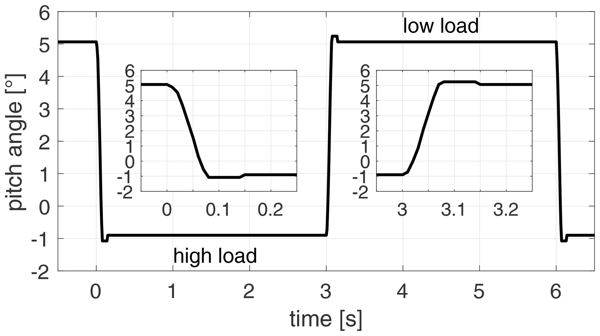
Figure 3Pitch motor encoder signal for a pitch step to high load followed by a step to low load with additional zoomed-in views of the actual pitch steps.
For the LDA measurements, 100 pitch steps were performed for each radial position and pitch direction at a typical sampling frequency of 600 Hz. This sampling frequency is just an order of magnitude estimate, since it depends on many parameters, especially the seeding of tiny oil droplets in the wind tunnel and thus varies constantly. Load measurements are taken during the LDA measurements. Therefore, load signals for 900 pitch steps are available. The hot-wire measurements have been performed separately. A wake rake consisting of four hot wires was used to measure at the described 56 positions in the wake. Thus, the experiment, consisting of 25 pitch steps, had to be performed times, and the wake rake was moved between those measurements.
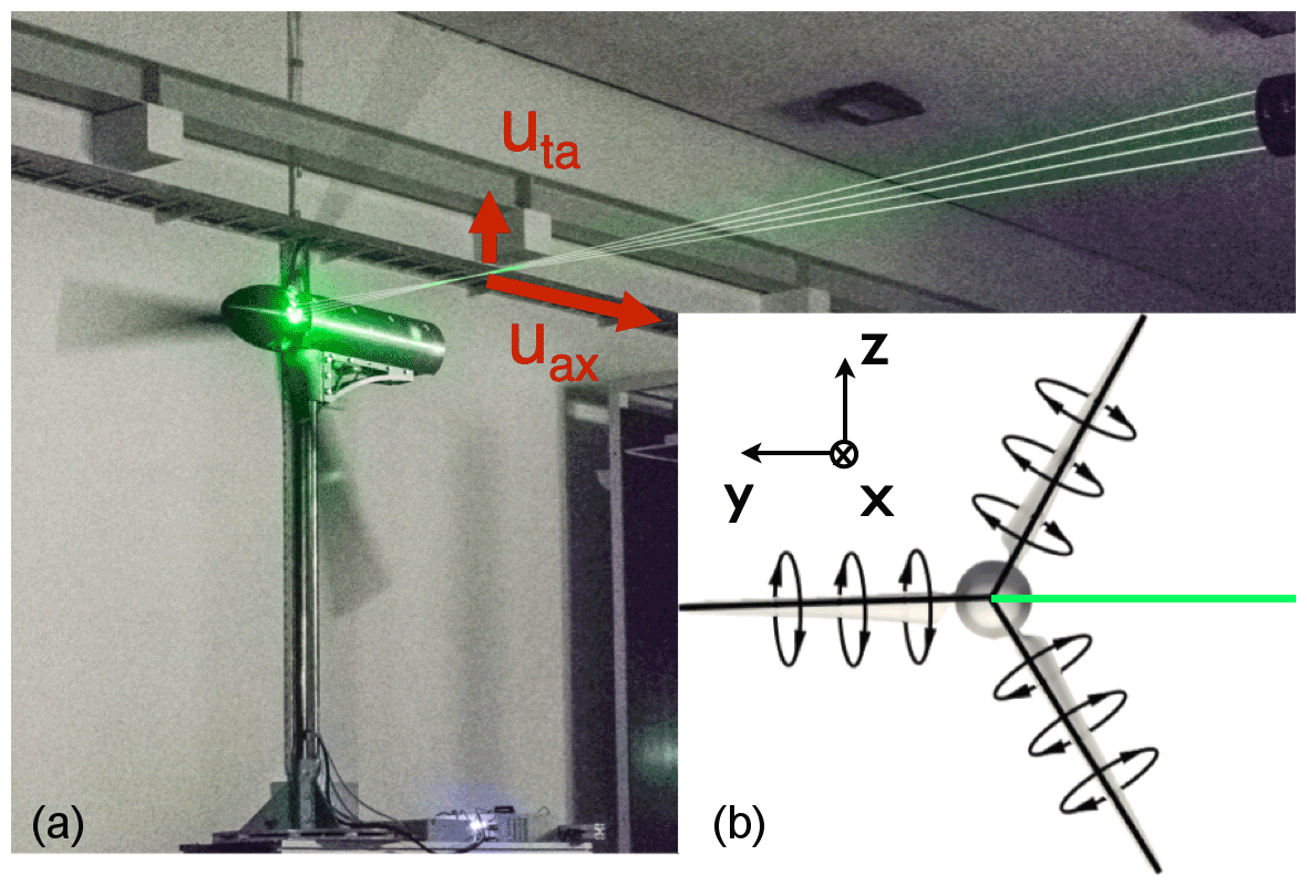
Figure 4(a) Clockwise-rotating MoWiTO 1.8 with 2D LDA probing axial uax (along x axis) and tangential uta (along z axis) velocity components in the bisectrix of two blades. (b) Scheme of counterbalancing bound circulation of the evenly loaded blades of front view of clockwise-rotating rotor. The LDA measurement line is indicated in green (adapted from Herráez et al., 2018).
2.1.3 Wake induction measurement by 2D LDA
The wake induction is derived from the LDA measurements by a method introduced by Herráez et al. (2018) for steady operation. The method uses the local velocity in the rotor plane, free of the influence of the bound circulation. This velocity is obtained by probing in the bisectrix of two rotor blades for axial and uniform inflow. In the bisectrix, the blade induction is counterbalanced and thus cancelled out.
In Fig. 4a the MoWiTO turbine is shown with the LDA laser beams and the probed axial (uax) and tangential (uta) velocity components at a specific radius. Alongside, in Fig. 4b, the concept of the counterbalancing of the bound circulation of the evenly loaded blades is sketched. For the shown position, the blade at the 9 o'clock position has no influence on the axial velocity on the indicated line of measurements. At that line, the downwash of the blade ahead of the indicated line counteracts the upwash of the blade behind it, and they cancel each other. The velocity at the line thus is only influenced by the wake induction. Herráez et al. (2018) argue that the trailed vorticity, especially at the tip, might play a non-negligible role, as it cannot be captured well at the high distance between the measurement position and the blade tip. Therefore, the method is less suited for the root and tip region of the blade.

Figure 5(a) Measurements of axial probe for high load case at a radius of 0.7 R for 400 revolutions over azimuth angle ϕ1 with marked data within the bisectrix threshold. ϕ1=0∘ relates to the 12 o'clock position of blade 1; (b) analogously for the tangential probe.
Two constraints defined the line of LDA measurements. The first is the height range of the LDA probe head, which is from tower bottom to hub height. The second is to minimise the influence of the tower on the blade nearest to the tower for the measurements in the bisectrix of two blades. This led to a measurement line at the 3 o'clock position. The tower does disturb the axial symmetry, however, based on an estimation of the tower effect with a dipole model as in Schepers (2012) the tower effect on the 5 o'clock blade position is considered negligible.
To obtain the values in the bisectrix, the LDA system is synchronised with the MoWiTO data acquisition system. Measurements at the constant high load are plotted for one position of the axial and tangential probe over the azimuth angle ϕ1 of the turbine in Fig. 5. The bisectrix values that are in a threshold of ±3∘ are marked in red. These threshold values were identified to give a good compromise between data points and data quality.
In Fig. 5a the analytical course seen by the axial probe according to Herráez et al. (2018) (see Appendix A) is presented and shows a good match to the measured signal. This good fit gives a high level of confidence to the applicability of the method to this experiment. For the tangential probe, data are missing around −1.3 m s−1 and also at 2.3 m s−1 for the axial probe, which is due to the prototype status of the LDA software at that point in time. We were aware of this bug, and it has no influence on the presented measurements.
Based on these measured axial and tangential velocities, the undisturbed inflow velocity u0 and the angular velocity Ω and the axial (a) and tangential (a′) wake induction factors are defined by Eqs. (1) and (2). With the geometrical angle γ between the chord of the local blade segment and the rotor plane, consisting of twist and pitch, the angle of attack, α, can be calculated by Eq. (3).
The method was validated based on particle image velocimetry (PIV) measurements and CFD calculations of the MEXICO rotor by Herráez et al. (2018) for steady operation. They found a good performance of the method from 0.3 R up to 0.9 R. In Rahimi et al. (2018), the model was further compared to alternative approaches applied to CFD simulations. Based on these comparisons and the specific focus on the dynamic change of inductions, rather than the total values, the agreement at the root radius at 0.25 R and the tip radius at 0.95 R is considered still reasonably good. Therefore, it is decided to include these radii in this analysis. However, they should be treated with care.
2.1.4 Ensemble averaging
Ensemble averages are used for the LDA data, hot-wire and strain gauge measurements. The data of many repetitions are aligned, triggered by the pitch command. An average value at each time step is constructed out of this data, for the time span −0.5 to 3 s, with the pitch step starting at 0 s. For example, the ensemble average of the flapwise blade root bending moment Mflap is given by Eq. (4), with the counter of cycles n, total cycles N and the time t.
This approach can smooth out non-deterministic variations and also structural interactions. In Fig. 6a, the flapwise blade root bending moment for the step to low load is shown for single cycles and the ensemble average. As the pitch step is not aligned with the rotor position, the effect of the tower shadow, seen for the single cycles, is smoothed out for the ensemble average. The high number of 900 repetitions, due to the nine different LDA positions with 100 pitch steps each, leads to a very small 95 % confidence interval (CI), which would barely be visible in the plots; therefore, is not shown here or later load-related plots.
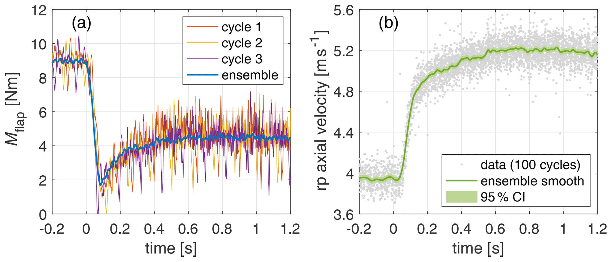
Figure 6(a) Single cycles and ensemble average of flapwise blade root bending moment Mflap. (b) Data points and smoothed ensemble average for axial rotor plane (rp) velocity in bisectrix of blades.
The induction factors have no fixed sampling frequency, as, firstly, the underlying LDA measurements are non-equidistant and, secondly, only values within the bisectrix of two blades are considered. To construct a single ensemble average out of this data, the 100 repetitions per LDA position are sorted to one signal, and a smoothing approach based on local regression and a weighted least squares and first-order polynomial model is used. For the local regression, 1 % of the data (length of the total dataset is 4.5 s) are used, whereas outliers get weight penalties and are not considered for more than 6 standard deviations. This filter is implemented as “rlowess” within MATLAB 2019b. These smoothed ensembled LDA-based data are resampled to 1 kHz, reducing the original non-equidistant data points by a factor of about 3. The sorted data points along the smoothed resampled signal and 95 % CI for the axial rotor plane (rp) velocity at 0.7 R for the step to low load are shown in Fig. 6b.
2.1.5 Corrections
Steady corrections are applied to the thrust and torque signals. For the torque, the mechanical torque is measured at the torque meter. To obtain the aerodynamic rotor torque, the friction in the bearings and the slip ring was calibrated by running the drivetrain without blades with the motor, used as a generator in operation; thus, the friction was measured with the torque meter. A linear function of the angular rotor speed was obtained and the respective value added to the signal.
The rotor thrust is derived from the tower bottom bending moment in fore–aft direction. The strain gauge was calibrated using defined forces in the thrust direction applied to the nacelle at the height of the rotor axis. The tower and nacelle drag was experimentally calibrated with the turbine without blades and was subtracted from the signal. The free stream velocity (u0) was used for this correction rather than a corrected wind velocity. This does lead to a small underprediction of the thrust. This error, however, is smaller as if no correction would be applied. In contrast to a dynamically corrected rotor plane wind velocity, this correction is a fixed value that does not influence the main shape of the dynamic load transient.
Dynamic corrections were considered for the torque and thrust signal. Directly after the pitch step, the torque control cannot keep the rotor speed completely steady, so there was a minor deviation of a maximum of 2 % of the rotor speed. Equation (5) is used to correct the torque by the contribution ΔM associated to the angular acceleration , where Irot is the equivalent rotational inertia of the rotor and drivetrain.
After the pitch step, there is an oscillation of the tower, which is seen in the tower bottom bending moment. The eigenfrequency of the tower and the damping constant of the oscillation is estimated iteratively and thus the measurement signal is corrected to obtain the aerodynamic thrust. The signals without the dynamic correction will also be shown in the results section as a reference (see Fig. 19).
2.2 Time constant analysis
The decay process after the pitch step is investigated in terms of time constant analysis. Firstly, a one-component time constant model (1c), like that used by Schepers and Snel (1995), is applied, given by Eq. (6) for the arbitrary signal S.
In Fig. 7a, the fitting approach is outlined for an exponential transition to a higher value without an overshoot, representing the behaviour that is expected from an induction transient. Figure 7b shows a signal with an overshoot and subsequent exponential decay to the new steady level. This represents the behaviour expected from a load. The fit starts when the pitch step is terminated at t0=0.070 s at the signal value . The new steady level after the pitch step is S1, being the mean value from t=2 s to t=3 s. The difference ΔS is given by and also contains the information on the direction. The time constant τsingle is fitted by means of the least root mean square error for the fitting range between t0=0.070 s and tfit=0.80 s.
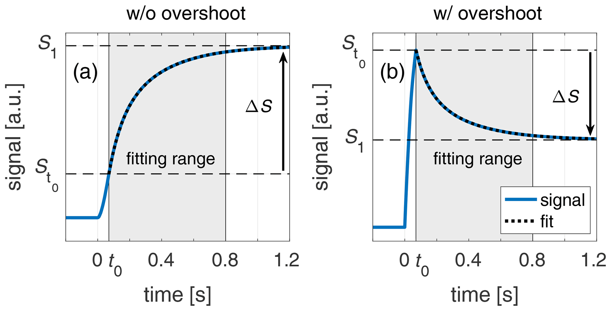
Figure 7(a) Time constant fitting scheme for a signal with exponential decay behaviour without an overshoot; (b) analogously for a signal with an overshoot.
Secondly, a model with two time constants (2c) similar to Sørensen and Madsen (2006) is used. The fitting model is given by Eq. (7). The fitting procedure is according to the single-time-constant model. However, three values are fitted: a fast time constant τfast, a slow time constant τslow and the weighting factor k of each exponential decay function, associated with the two time constants.
These time constants can be used for comparison and tuning of the time constants in the dynamic inflow engineering models of Øye (see Snel and Schepers, 1995), used in OpenFAST and GH Bladed, and the new DTU model (see Madsen et al., 2020), used in HAWC2. The time constants of these engineering models are derived from simulations and parameterised to the turbine size and operational conditions considering the relevant dynamic inflow time scaling factor , the radial position and the quasi-steady axial induction factor.
2.3 Load reconstruction from induction measurement
Additionally to the strain-gauge-measured integral turbine loads, these loads are also reconstructed based on the induction measurements. The angle of attack values along the rotor blade are already derived from the experiment through Eq. (3). The relative velocity urel is given by Eq. (8). Hence, the information obtained by the momentum part of a BEM code is known from the experiment. So the blade element theory (BET) part of a standard BEM code as outlined in detail by Hansen (2008) is used. The force for the blade segments can be calculated for the normal direction according to Eq. (11) and for the tangential direction according to Eq. (12), where the lift force of the segment is given by Eq. (9) and the drag force by Eq. (10). The inflow angle is defined by θ.
CL(α) and CD(α) are the lift and drag coefficients for the respective angle of attack. These lift and drag polars are obtained by XFoil (see Drela, 1989). The lift polars are corrected for 3D effects, as lift coefficients on rotating blades can be significantly higher than for a stationary blade due to the effect of cross-flows related to a stall delay. This effect is most relevant for the root airfoils and was corrected by the method by Snel et al. (1993). The blade segment width is Δr, and c the chord length. The air density is given by ρ. The factor F accounts for the tip losses based on the Shen et al. (2005) tip loss model. The integral load signals are reconstructed by integration of the forces along the rotor blade.
The influence of unsteady airfoil aerodynamics (uA) on the blade level, namely the Theodorsen effect, is not contained in the axial wake induction and therefore has to be additionally considered in the reconstruction. The implementation given in detail in Pirrung et al. (2017) is used. This is the inviscid part of the unsteady aerodynamics model by Hansen et al. (2004), which treats the shed vorticity effects due to fast angle of attack changes as a time lag on the angle of attack α and has been extended to take the effect of camber into account. Thus, the magnitude and direction of the aerodynamic forces are influenced. The main model is reproduced in Appendix B. The typical uA time constant which determines the lag of the angle of attack due to the uA effect is of the order of , whereas the typical time constant of the dynamic inflow effect is and at least 2 magnitudes of size larger, as mentioned in Sect. 1. Reconstructed loads will be investigated with and without the uA model.
Here the measurement results are described. In Sect. 3.1 the induction in the rotor plane is shown as a function of radial position determined with the procedure described in Sect. 2.1.3. Then Sect. 3.2 shows the wake measurements from the hot wires as a function of streamwise position at hub height. Finally Sect. 3.3 presents the loads as measured from the strain gauges and the loads derived from the induction measurements according to the procedure of Sect. 2.3.
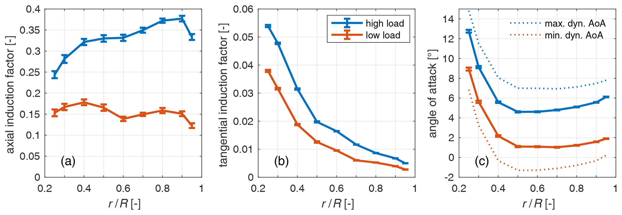
Figure 8(a) Axial and (b) tangential wake induction factors and (c) derived angle of attack distribution from the LDA measurements for the steady high and low load cases. The error bars denote the 95 % confidence interval, based on the measured data for axial and tangential velocity in the rotor plane considering 100 measurement cycles.
3.1 Induction results
In Fig. 8a, the measured axial inductions, in Fig. 8b, the tangential inductions and in Fig. 8c, the derived angle of attack from the LDA measurements are presented for the steady high and low load cases.
For the high load case, the axial induction has values between 0.25 near the root (0.25 R) and 0.38 near the tip (0.9 R), in general with an increasing trend with radius apart from the tip nearest radius. The low loaded case has a more uniform loading with values between 0.12 and 0.18. For comparison, the rotor equivalent axial induction obtained from momentum theory () with CT based on the strain gauge measurements do give similar values of 0.34 and 0.14 respectively.
The tangential induction for both cases is high near the root and decreases with radius with a high rate in the beginning and then more gentle. Due to the larger rotor torque, the high load case shows higher values.
The angle of attack distribution for the high load and low load cases shows angles of attack of 4 to 6∘ for the high load case from 0.4 R on and 1 to 2∘ for the low load case. The values increase towards the root for both cases. The stall angle is estimated as the angle of attack with the highest lift coefficient, where the flow is not completely separated. This angle for the used airfoils at the respective Reynolds number of the experiment is at 15∘ for the root airfoil used up to 0.4 R and at 11.5∘ for the tip airfoil used from 0.5 R on. Thus, the considered range of the blade is operating outside of the stall regime for both load levels for the steady states.
The observed difference between the two angle of attack distributions is smaller than the pitch step value of 5.9∘ the blades do pitch. This is due to the flow through the rotor and induction factors that change between the two steady operational states. From this information, the maximum angle of attack range can be estimated a priori, in order to assess the flow conditions during the pitch steps. The dynamic maximum and minimum angle of attack distributions are estimated for an infinitely fast pitch step. We assume in a thought experiment that the flow field of the steady state before the pitch step is unchanged, but the pitch step and thus geometrical change of the inflow angle is already done. This allows us to estimate the extreme dynamic angles of attack, neglecting any damping uA effects for the infinitely fast pitch step.
These maximum and minimum dynamic angles of attack are shown as dotted lines in Fig. 8c. For the step to high load, the stall limit is approached at nearly 15∘ angle of attack at the root near radius of 0.25 R. For the step to low load, there is a minimum dynamic angle of attack of about −1.5∘ in the middle of the rotor blade. This lowest angle of attack gives a lift coefficient of zero. For a finitely fast pitch step, the flow already adapts during the pitch step and the extreme dynamic values are closer to the new steady values. The uA effects further dampen the overshoot of angles of attack. So apart from the blade root at the step to high load, where the stall limit is approached, the blade is operated outside the stall region for the pitch steps.
The axial induction factor transients are shown in Fig. 9 for four different radii (0.3, 0.5, 0.7 and 0.9 R) for both pitch steps. They show direct evidence of dynamic inflow where the induction factors and therefore induced velocities reach the new equilibrium value only slowly.
The fits of the one-time-constant (1c) and two-time-constant (2c) models are also shown in the plots. The fits start from the instance the pitch step is terminated at t0. At that time the axial induction has already adapted by about 28 % on average of the difference between the steady axial induction levels for the radii from 0.3 to 0.9 R independent of the pitch direction.
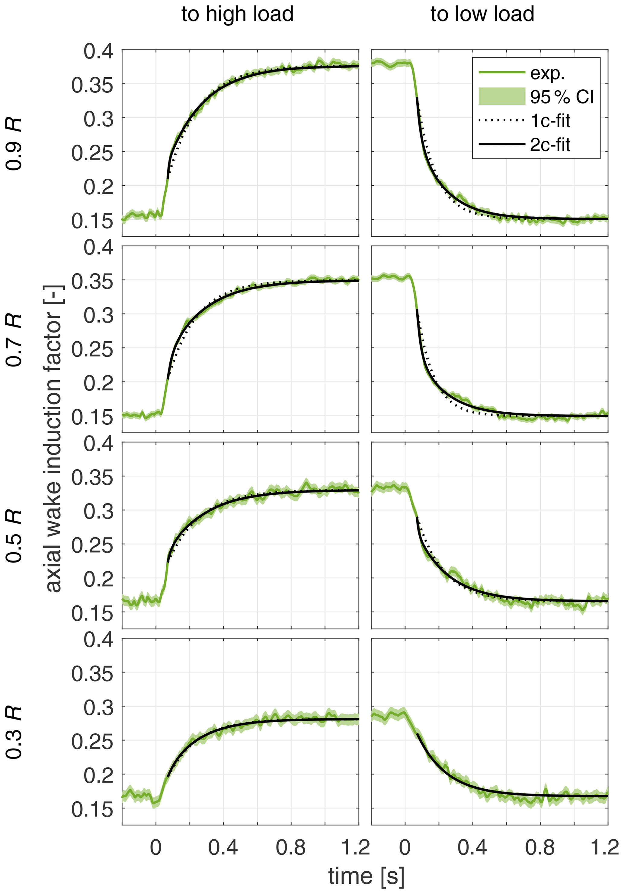
Figure 9Axial wake induction factor over time for pitch step to high load and low load for the four radii 0.3, 0.5, 0.7 and 0.9 R and the fitted exponential decay models with one time constant (1c) and two time constants (2c).
The fitted time constant τsingle of the 1c model is plotted over the radius for both pitch directions in Fig. 10. In the root near region up to 0.4 R both pitch directions show similar values apart from the radius at 0.25 R, where the step to high load has a higher time constant. For radii from 0.5 R on, the step to high load shows higher values than the step to low load. There is no clear trend obvious for the step to high load. In contrast, for the step to low load, there is a trend towards reduced time constants towards higher radii.
In Fig. 11, the three fitting parameters of the 2c model are presented. In the top row, the three fitted variables k=kfree, τfast and τslow are plotted over the radius. Near the root at 0.25 R, the k value for both pitch directions has a value of 1 and nearly 1 respectively, indicating no contribution from τfast, which consequently is also not plotted for these radii. For radii up to 0.5 R, the values for the step to low load have a higher kfree value than for the step to high load, switching from 0.6 R on to the tip. τfast does have similar values from 0.4 R to the tip and for both pitch directions. Towards the root the decay process is only defined by τslow there, as kfree equals or nearly equals 1. For τslow, there is no clear radial trend for both pitch directions, but a clear difference between pitch directions. For the step to high load, τslow is higher for all radii than for the step to low load. Due to the influence of the varying weighting ratio of fast and slow time constant, a direct comparison of these time constants is limited.
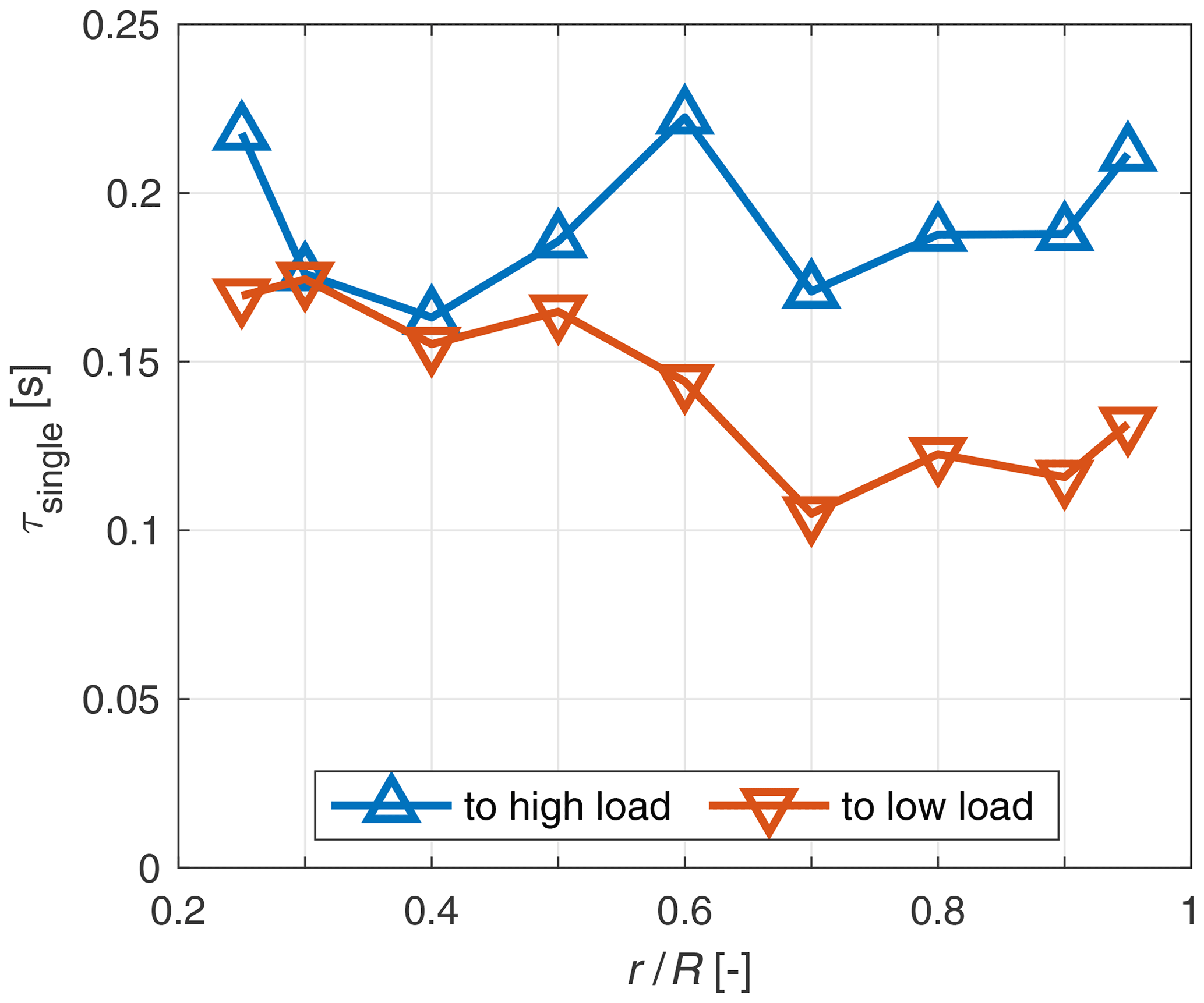
Figure 10One-time-constant model fit of τsingle to the axial wake induction factor over the radius for both pitch directions.
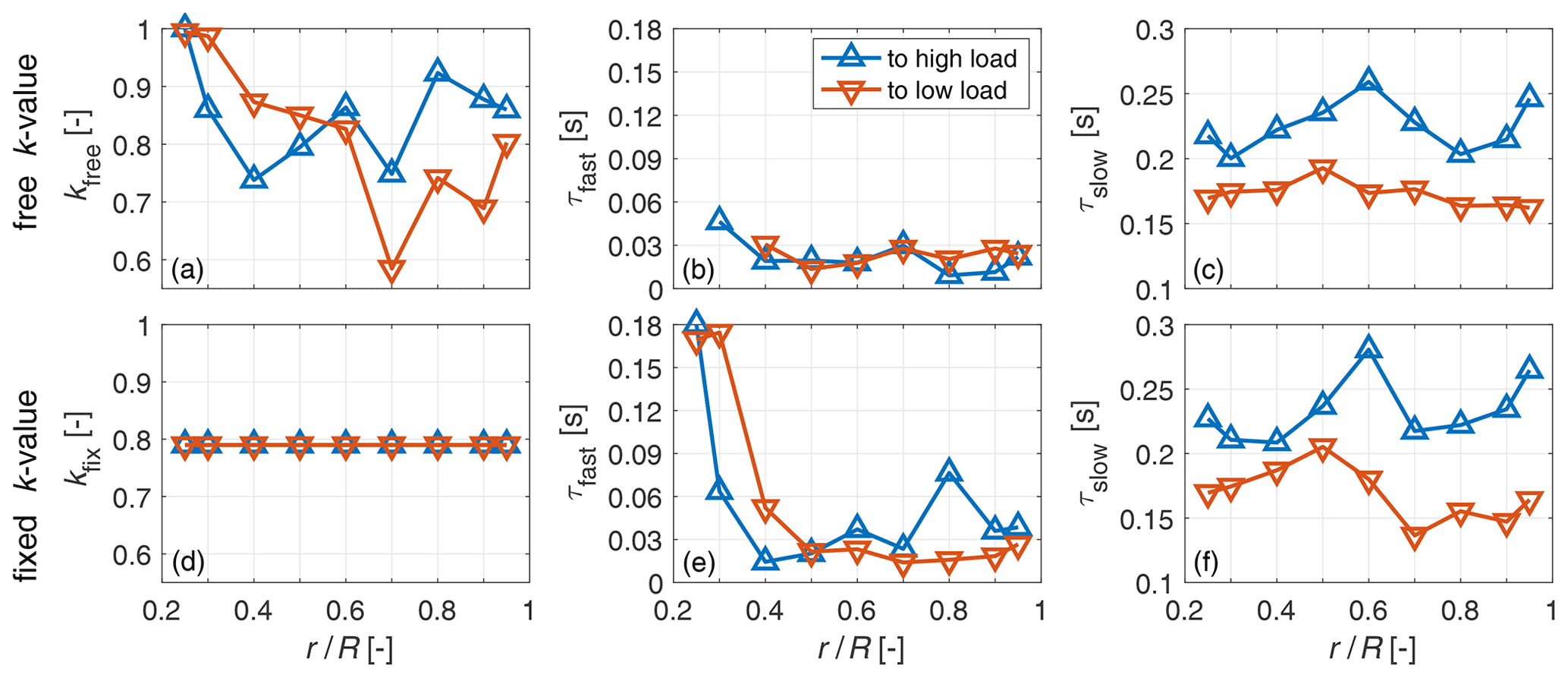
Figure 11Two-time-constant model fit to the axial wake induction factor, derived from the rotor plane LDA measurements with the ratio k and the fast τfast and slow τslow time constants. In the top row the k value is fitted as a free parameter. In the bottom row the weighting ratio of fast and slow time constant k is fixed (to the mean value of both pitch directions and radii of the fit in the top row).
To overcome this limitation, the ratio k is fixed to a value of kfix=0.79, which is the mean value for all radii of both pitch directions of kfree. With this setting, τfast contributes by 21 % to the decay of the axial induction. This fit is shown in the bottom row of Fig. 11.
The fitted τfast is high near the root for both pitch directions. For the step to high load, τfast decreases from the root to 0.4 R, after which there is an increase again (ignoring an outlier at 0.8 R). From 0.5 to 0.9 R, τfast increases by 67 %. For the step to low load, τfast has more constant values from 0.5 to 0.9 R, decreasing by 14 %. Hence τfast is smaller for the negative load step, for radii larger than 0.5 R, which represents 75 % of the rotor swept area.
Values of τslow are slightly higher for the step to high load and show more variation than in the prior fit with k=kfree ratio. There is a slight radial trend to higher values, with an increase in τslow from 0.3 to 0.9 R by 11 %. For the step to low load, also more variation is apparent, and a slight radial trend towards lower values is indicated, with a decrease in τslow from 0.3 to 0.9 R by 16 %. Taking the mean value over radius, the slow time constant for the step to low load is about 28 % lower.
The fitting accuracy of the applied models is determined based on the root mean square error (RMSE) in the fitting range t0 to tfit between the measured signal and the respective fitted model and plotted over the radius in Fig. 12.
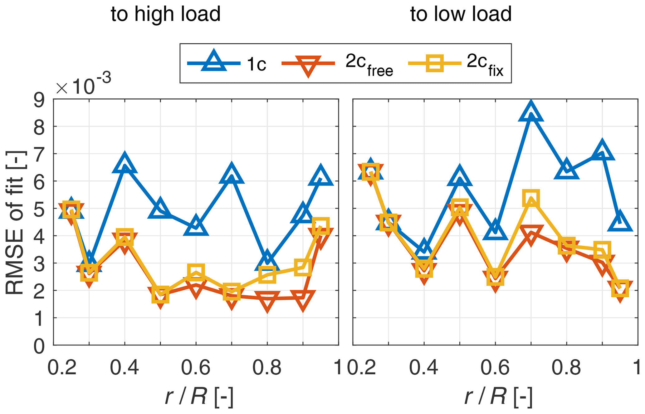
Figure 12Root mean square error (RMSE) between measured axial wake induction factor and the three fitted models, 1c-fit and 2c-fit with kfree and kfix for both pitch directions.
For both step directions, there is no difference in RMSE for the root near stations up to 0.3 R between the fitting models, which are the 1c and 2c model, one with k=kfree and one with k=kfix. For higher radii, the error of the 1c fit is higher than for the two variants of the 2c model. The differences between the two variants of the 2c model are small, showing that there is only a small penalty for fixing the k ratio.
The tangential wake induction factors over time for both pitch directions are presented for the four radii 0.3, 0.5, 0.7 and 0.9 R with the fit of the 1c model in Fig. 13.
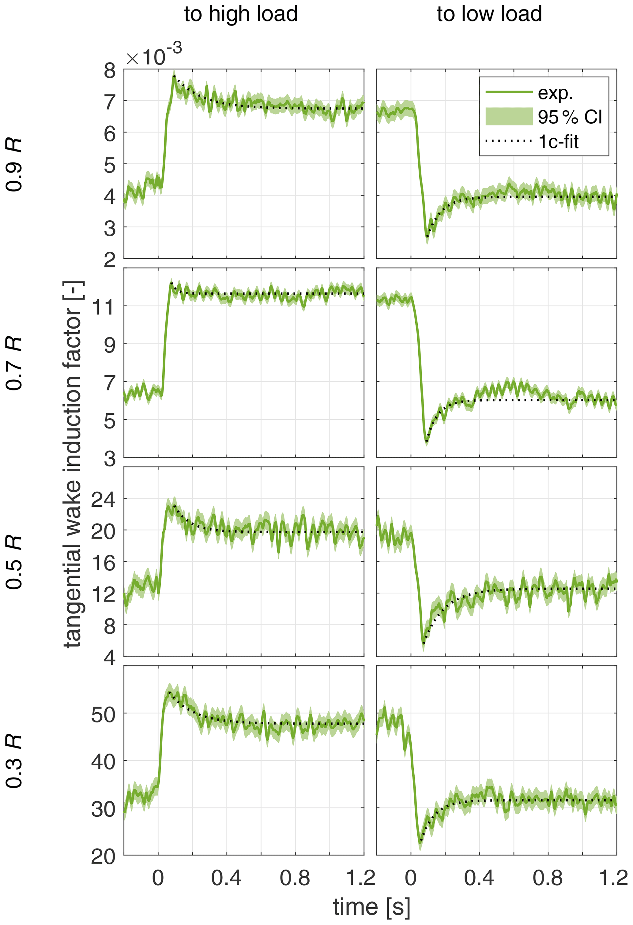
Figure 13Tangential wake induction factor over time for pitch step to high load and low load for the four radii 0.3, 0.5, 0.7 and 0.9 R and the fitted exponential decay model with 1 time constant (1c).
In contrast to the axial induction, the tangential induction shows an overshooting behaviour. The exponential fit starts around t0 at the respective minimum or maximum peak, as this showed to improve the fitting. The starting point of the fit thus varies between 0.059 and 0.095 s, with a mean value of 0.074 s. The overshoot, in general, seems more prominent for the step to low load and only barely present within the signal noise at the radius of 0.7 R for the step to high load.
The fitted τsingle values to the 1c model are plotted over radius for both pitch directions in Fig. 14. Cases where the overshoot is smaller than 3 standard deviations of the filtered signal of the new equilibrium were excluded due to a very high sensitivity on the starting point of the fit.

Figure 14One-time-constant model fit of τsingle to the tangential wake induction over the radius for both pitch directions.
For the step to high load, only two radii at the root and two radii near the tip fulfil this requirement, whereas for the step to low load only the tip most radius at 0.95 R is excluded. For the radii where values for both pitch directions are available, the step to high load shows higher τsingle values. For both pitch directions, τsingle is lower than the corresponding τsingle for the axial inductions. We see no connection of this unexpected overshooting behaviour of the tangential induction to the slight rotor speed deviations, which are present between 0 and 0.6 s and thus at a time frame up to 1 order of magnitude higher.
The influence of the small, allowed shift in the start of the fit is also investigated. For a strict starting point of the fit at t0, shown in Fig. 14 as stars, the set criterion of overshoot to noise is fulfilled for only three radii for the step to high load and five radii for the step to low load. For the available radii, however, there are only negligible differences to the shown fit in comparison to the observed spread.
3.2 Wake results
In the following the hub height hot-wire measurements downstream of the turbine in the near and close far wake up to 2 D downstream are analysed. The wake measurements are shown as a surface plot for four different timestamps in Fig. 15 for both pitch directions and normalised by the free stream velocity.
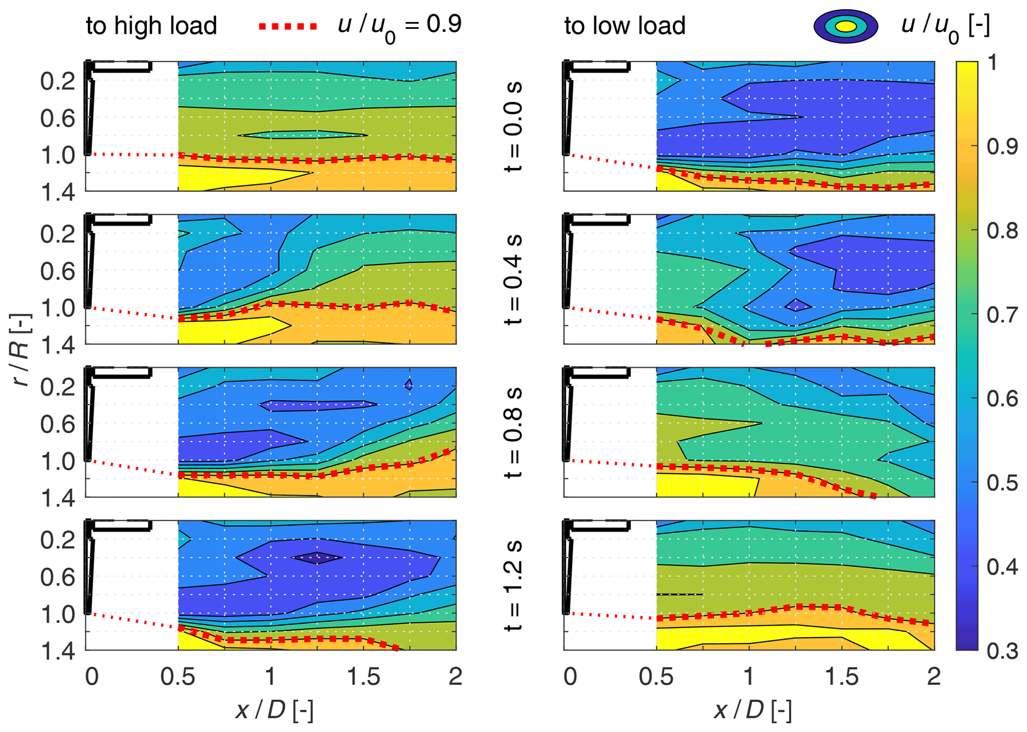
Figure 15Top view on velocity contour in the horizontal plane at hub height of the wake at the four different timestamps 0, 0.4, 0.8 and 1.2 s after the pitch steps to high and to low load, normalised by the free stream velocity. The turbine dimensions are indicated in correct scale in the plots as a reference, with the x axis being the axis of rotation.
The first contours at t=0 s are the starting equilibrium condition. For the step to high load, the initial wake, being the steady low-load case, shows wake velocities around 0.8 u0 coloured in green tones for 0.2 to 1 R radial positions. For the step to low load, the initial velocity field in the wake, being the steady high-load case, is around 0.5 u0, coloured in blue tones. The dotted red line is the isoline of 0.9 u0, which is used as an indication of the wake stream tube.
The contours for the following timestamps show the transition to the new steady state. These transitions seem at first glance different for the two pitch directions. For both pitch directions at t=0.4 s and at around 1 to 1.25 D, there seems to be the transition line where old and new wake meet. The indicated wake radius shows that the dynamic wake streamtube is constricted at 1 D for the step to high load, whereas it is widened up for the step to low load. This behaviour is opposite to what is expected for the new steady streamtubes, where for the step to high load, the wake widens, due to the higher thrust. Further, it narrows due to the lower thrust for the step to low load. For the time stamp at t=0.8 s, a similar picture can be seen where this transition between old and new wake has progressed to around 1.75 D. The figure at the left bottom is very similar to the figure at the right top, and the same holds for the figure at the right bottom and left top. This indicates that the new equilibrium is approached at t=1.2 s.
To further interpret this measurement, normalised velocity contours are presented to the new equilibrium steady state in Fig. 16. The normalised difference is defined as , with , where ut is the velocity at the respective time at a measurement position, and u∞ the velocity at the same point at the new steady condition after the pitch step.
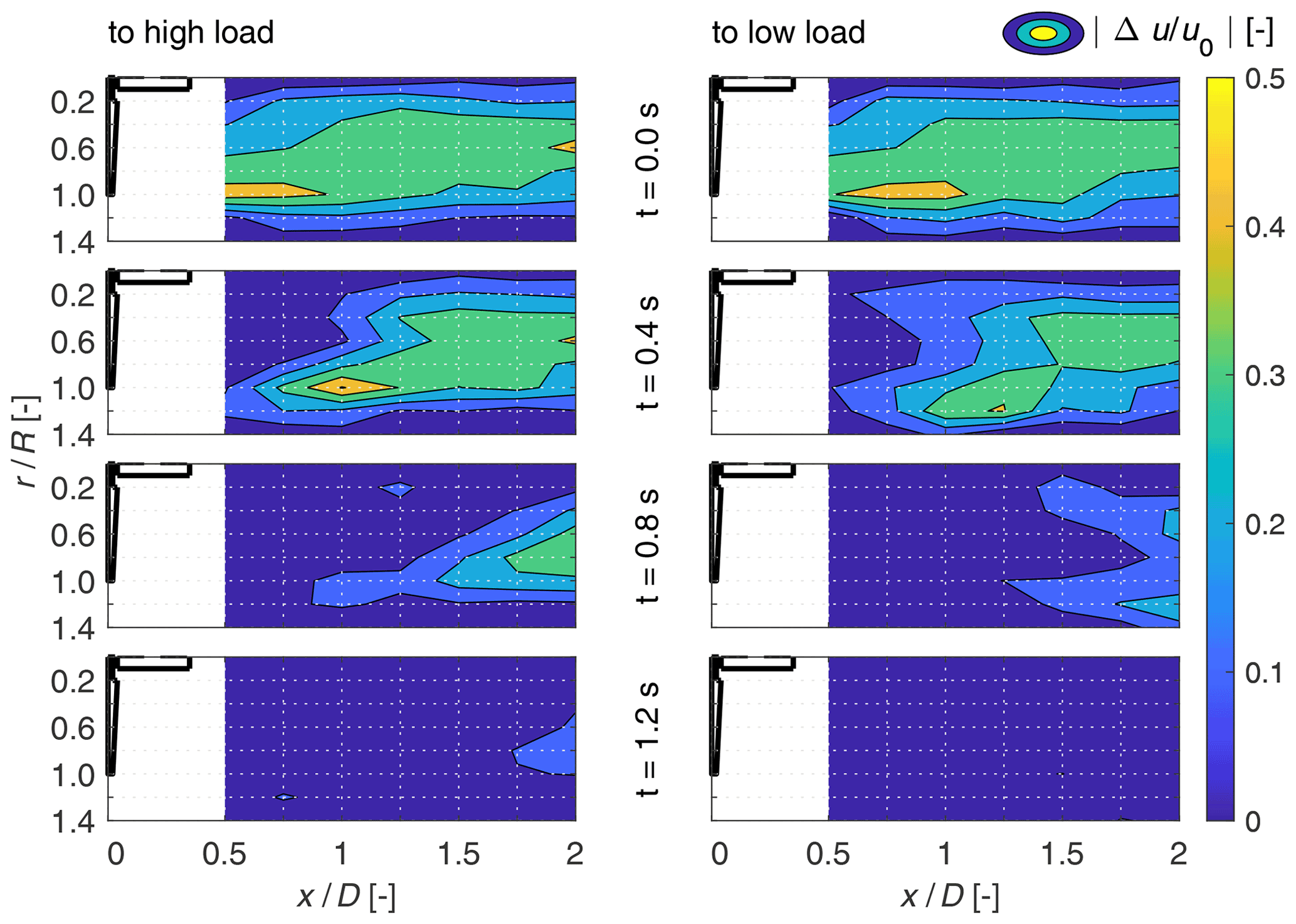
Figure 16Top view on velocity contour in the horizontal plane at hub height of the difference to the new steady wake equilibrium at the four different timestamps 0, 0.4, 0.8 and 1.2 s after the pitch steps to high and to low load, normalised by the free stream velocity. The turbine dimensions are indicated in correct scale in the plots as a reference, with the x axis being the axis of rotation.
Therefore, a value of 0.5 means that the wake has to adapt by 0.5 u0 to reach the new equilibrium. The starting conditions for both pitch directions look alike, as they show the difference between the two steady states. At the timestamp of t=0.4 s, a very similar shape of this potential like area is seen for both pitch directions. A widening of the wake for the step to low load is indicated when concentrating on the orange field near the tip radius, which is at a radial position of 1 R for the step to high load and at 1.2 R for the step to low load. For the step to low load, this orange maximum has travelled further than for the step to high load. At the timestamp at t=0.8 s, the wake for the step to low load has adapted more to the new steady state than for the step to high load. At the timestamp of t=1.2 s, for the step to low load, the equilibrium is reached. For the step to high load, the wake has not completely adapted to the new equilibrium with still a clear lighter blue area at 2 D.
Next, the deployment of the axial wake velocity as a response to the load steps is analysed. Six of the hot-wire signals used to make the contour plot are plotted over time for the step to high load for the radii of 0.2, 0.6 and 1 R at 0.5 and 1.5 D distance behind the turbine are presented in Fig. 17.
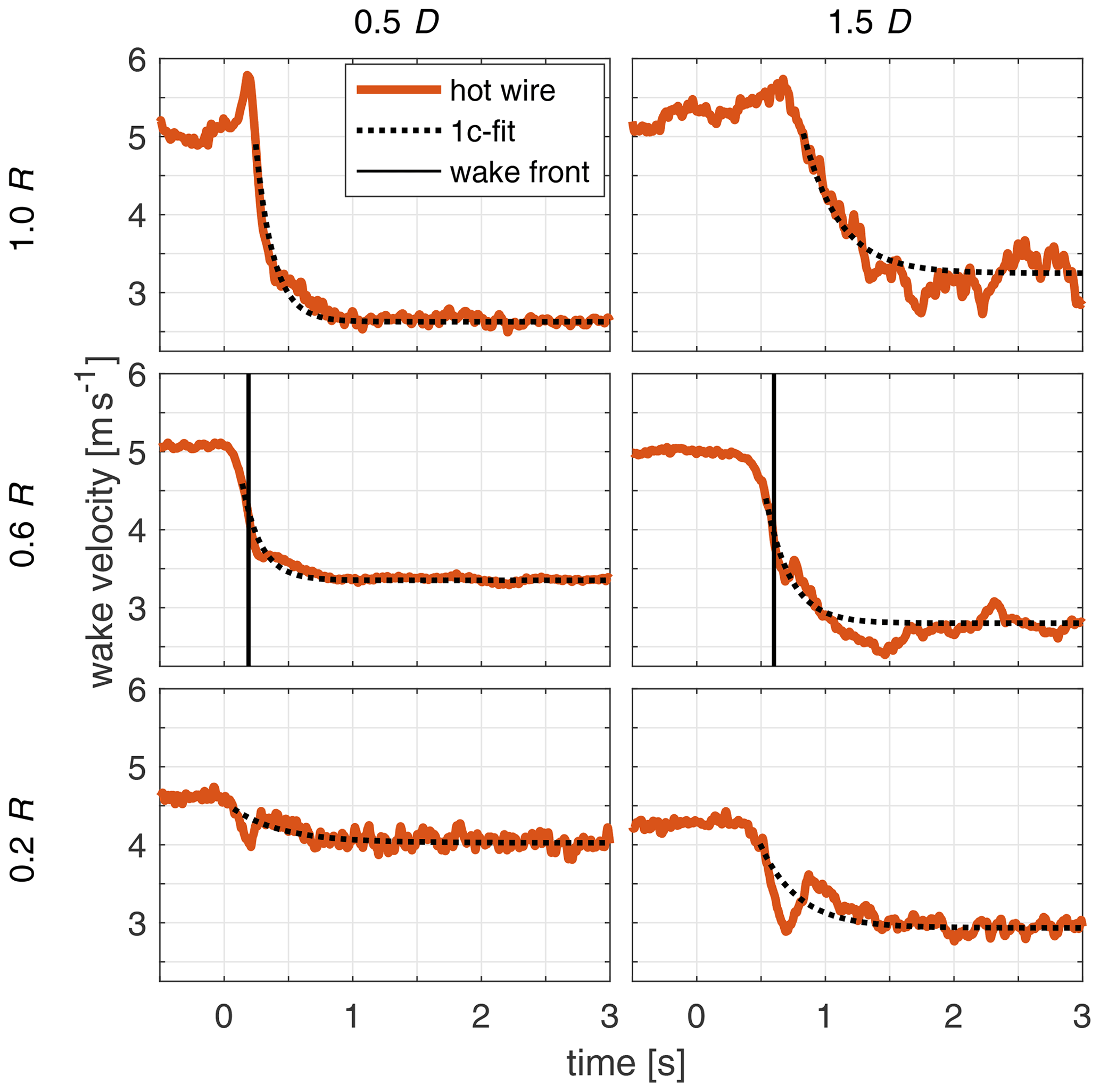
Figure 17Ensemble averages of the axial wake velocity measured by hot wires for the three radii of 0.2, 0.6 and 1 R at 0.5 and 1.5 D distances behind the turbine for the step to high load.
For the radius at 0.6 R, a vertical line, called a wake front, marks a characteristic t1 of the exponential decay, where the signal has adapted by 50 % to the new equilibrium value. For the radius of 0.2 R, the velocity transient shows a local structure, where the velocity quickly decreases and increases again to subsequently decrease to the new equilibrium for both shown distances. The effect of the nacelle is assessed as unlikely to be the reason for this structure, as the nacelle only has a radius of 0.1 R. At the radius of 0.6 R the signal decays exponentially. At 1 R the signal increases quickly to a peak at nearly free stream velocity before decreasing exponentially to the new steady value. The signals at 0.5 D behind the turbine for the two higher radii, 0.6 and 1 R, show a better fit with the exponential decay function. For the farther distance at 1.5 D, the hot-wire signals show an overshoot to lower velocities than the new equilibrium at around 1.5 to 1.7 s for the two larger radii. The results for the indicated time constant fit are presented and discussed as an additional result in Appendix C.
In the next step, the wake front velocity is analysed to measure how fast the transition point (the wake front) between the old wake and the new wake convects. This wake front can be thought of as being similar to a weather front. We define the wake front velocity by the time this characteristic wake front needs to travel from one considered downstream position to the next. So exemplarily in Fig. 17 at 0.6 R there is the wake front for 0.5 D at s and for 1.5 D at s. Within this time difference, the wake front thus has travelled by 1 D, giving a mean wake front velocity between these downstream distances.
In Fig. 18, this wake front velocity is shown for both pitch directions, normalised by the free stream velocity. The wake front velocity is obtained by considering a mean value of the hot-wire positions at the radii of 0.4 , 0.6 and 0.8 R. These signals were weighted based on their position with the conservation of mass in mind. For that, each position was attributed an annulus reaching ±0.1 R from the radius of the position. This mean velocity signal at the different downstream distances, which is used to obtain the wake front velocity, represents in this definition (0.3 to 0.9 R) the major part of the swept area of the rotor.
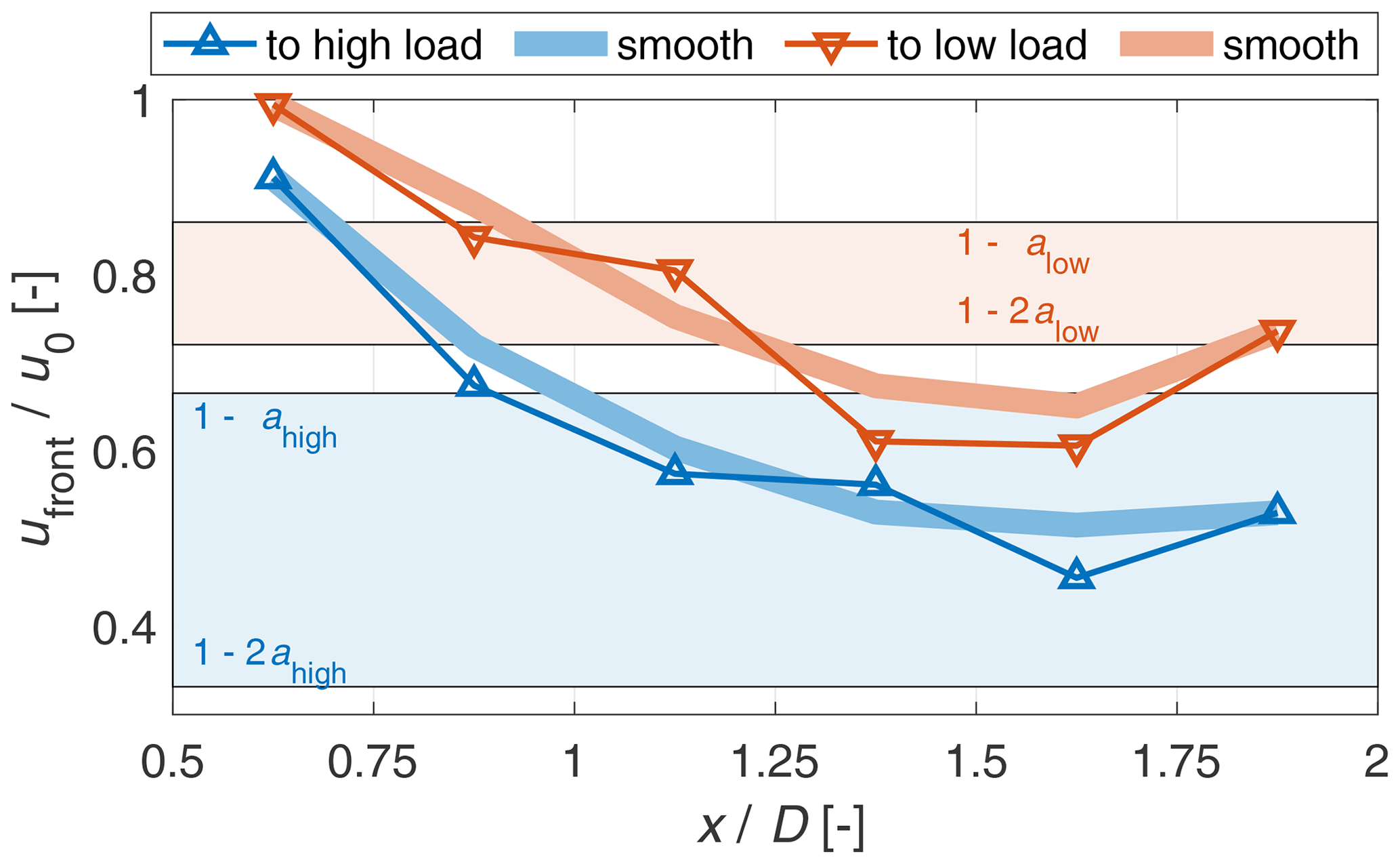
Figure 18Velocity of the wake front for both pitch directions, normalised by the free wind velocity. For orientation, also the theoretical normalised wind velocity in the rotor plane (1−a) and in the far wake (1−2a), based on the measured thrust coefficient, are indicated for both steady states.
Thus between every two considered downstream distances a mean velocity with which the wake front moved can be calculated. Between the two nearest distances to the rotor, 0.5 and 0.75 D, the wake front convects for both cases with 0.9 u0 to u0. This is faster than the expected velocity in the rotor plane for even the low loaded rotor. With increasing distance to the rotor for both cases, the wake front velocity decreases up to 1.5 D, whereas the velocity is higher for the step to low load. Based on this defined wake front velocity the wake convection is on average 26 % faster for the step to low load.
3.3 Load results
Next, the integral loads are compared as shown in Fig. 19. Two independent methods have been used: One measured directly with strain gauges (SGs) and one obtained indirectly from the LDA measurements in the rotor plane with the reconstruction procedure given in Sect. 2.3 (denoted LDA recon.). For the latter, it is distinguished between the use of the uA model and without it. For the strain-gauge measurements, additionally a version without the dynamic corrections for Fthrust and Maero (denoted SG no corr.) as introduced in Sect. 2.1.5 is presented to show the raw data. For the reconstructed loads, the influence of unsteady airfoil aerodynamics (uA) effects is shown around the overshoot, where it differs from the case without the uA model.
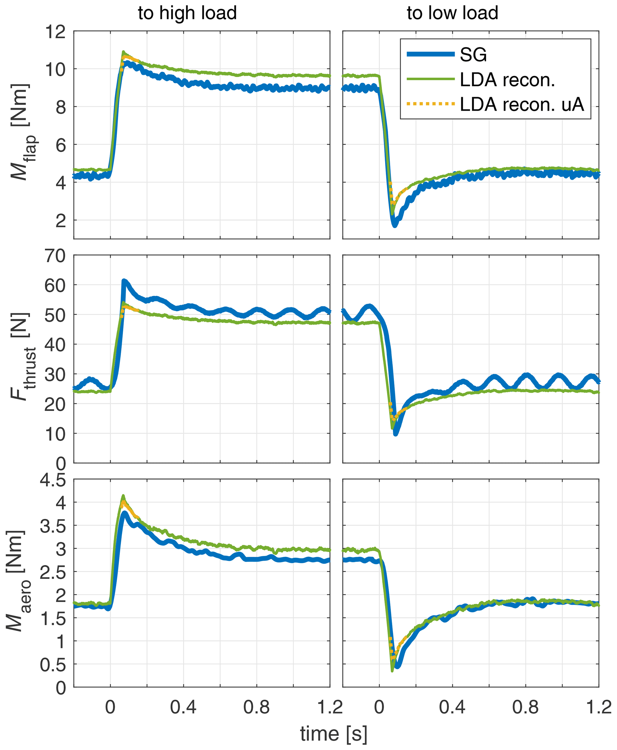
Figure 19Integral turbine loads based on strain gauges with (SG) and without (SG no corr.) the dynamic corrections (as introduced in Sect. 2.1.5) and reconstructed loads based on Blade Element Theory from the LDA measurements without and with uA model.
Firstly, a clear overshooting behaviour of all load signals is apparent. Comparing the strain gauge measurements for Mflap, Fthrust and Maero with the signals reconstructed from the LDA measurements indicates a good match of signals by means of steady values as well as the dynamic overshoot. Considering the uA model leads to a peak shaving of the overshoot. Also, the overshoot peak for the strain gauge signals, as well as for the reconstructed value with the uA model, is slightly shifted to higher t0 values.
A more detailed comparison of the steady values at high and low loads between the strain-gauge-measured integral loads and the reconstructed loads is plotted in Fig. 20, alongside the deviations of the reconstructed loads to the strain-gauge-measured loads. The two methods give similar load levels. Deviations differ between the load signals. The good agreement in terms of steady loads indicates good performance of this reconstruction approach with maximum deviations of 11 %.
The slight overprediction of reconstructed loads for the Mflap and Maero, on the one hand, and the underprediction of Fthrust is attributed to a higher influence of the larger radii. For the first two signals, the blade acts as a lever arm for the sectional forces, thus giving them a higher weighting. In contrast, the sectional forces are added without considering a lever arm for Fthrust.
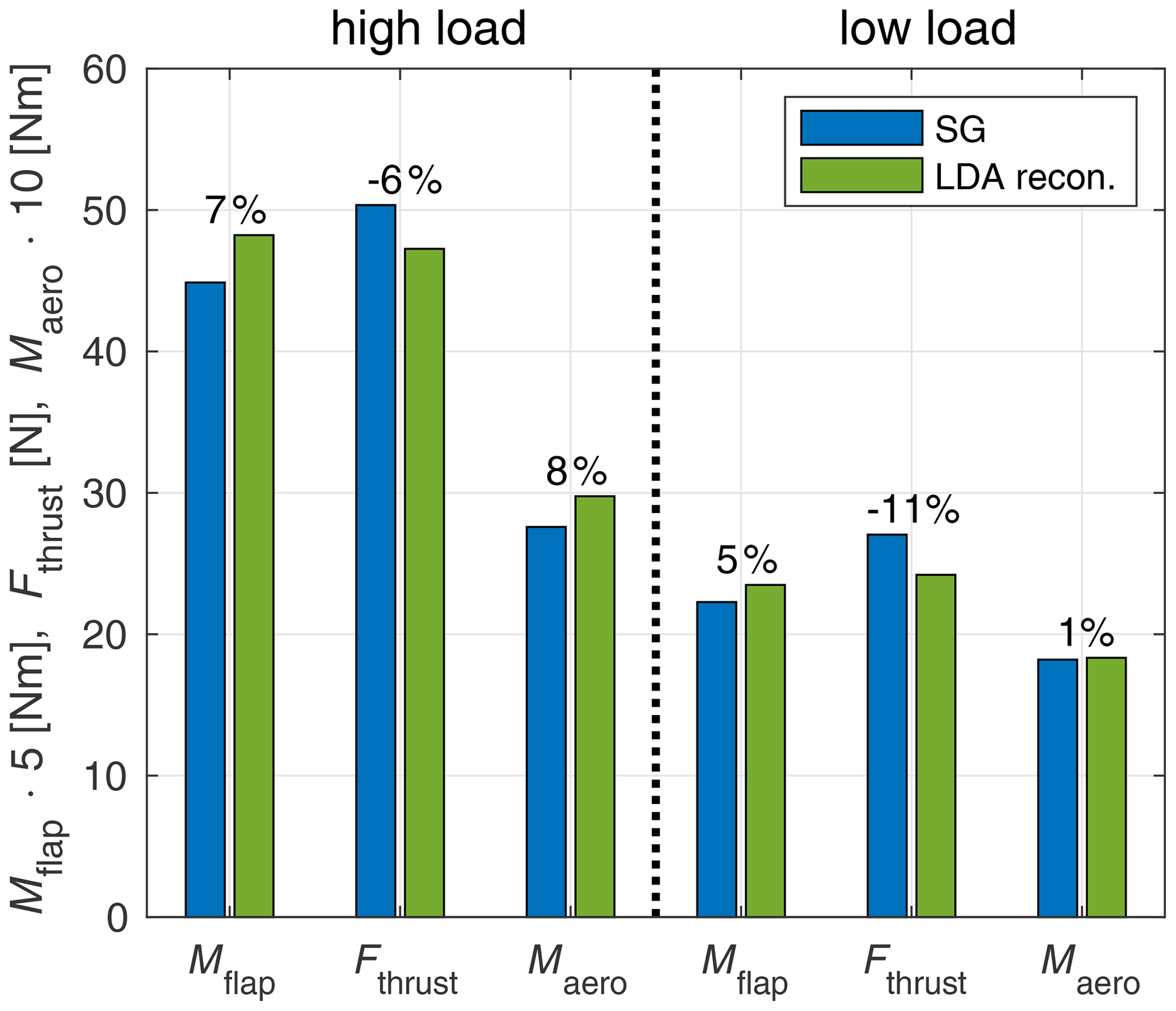
Figure 20Comparison of the steady load levels for high and low loads for the integral turbine loads Mflap, Fthrust and Maero obtained by strain gauges and reconstructed from LDA measurements.
Further, the dynamics after the pitch step are compared. The amount of load overshoot, normalised by the difference between the steady values, is given for the load signals for both pitch directions in Fig. 21a.
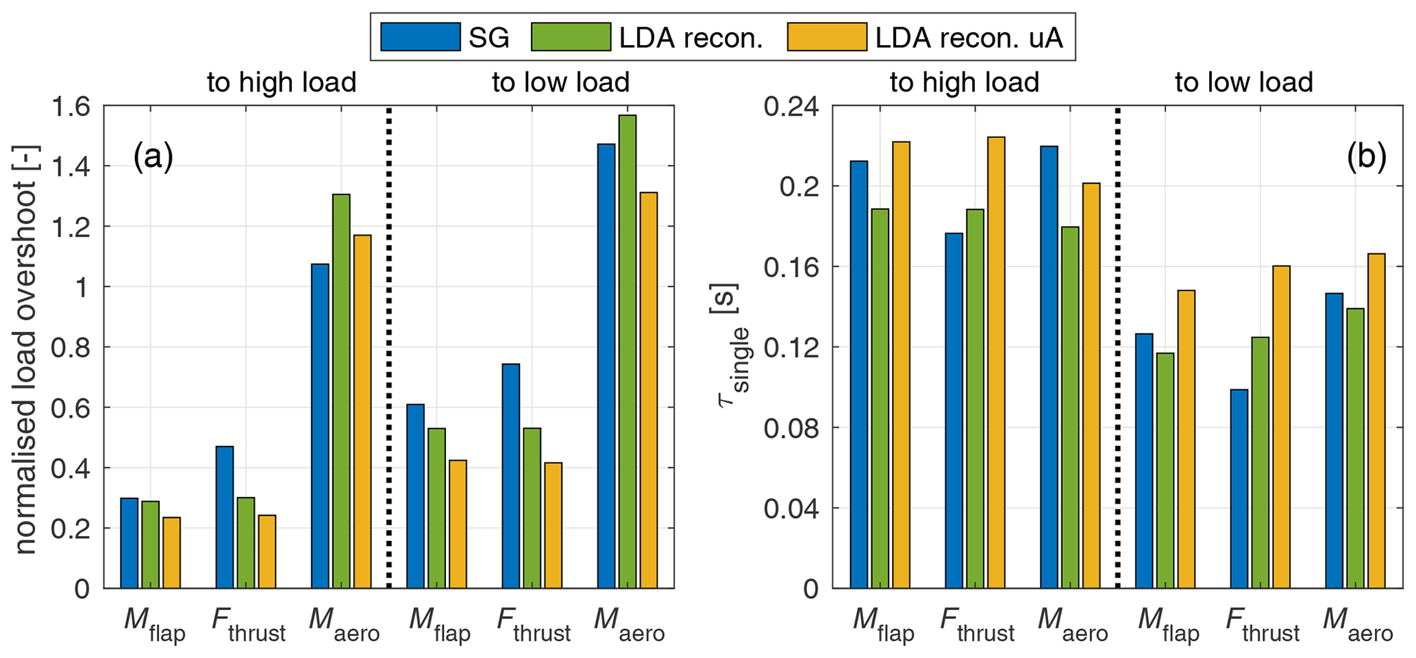
Figure 21(a) Comparison of the amount of overshoot of the integral turbine loads Mflap, Fthrust and Maero, obtained by strain gauges and reconstructed from LDA measurements without and with uA model for both pitch directions. (b) Comparison of the τsingle fit of the one-time-constant model to these integral loads.
The addition of the uA model reduces the amount of overshoot for all load channels. For Mflap, the reconstructed loads provide a good fit, whereas the values with uA model show differences. High deviations are seen for Fthrust between strain gauge measurement and reconstructed loads, especially with the uA model but also without the model, for both pitch directions. The torque Maero shows a good match with the reconstructed loads for both pitch directions.
The amount of overshoot is higher for the step to low load, when comparing the amount of overshoot between the two pitch directions per load channel and method. Based on the LDA reconstructed loads, which are not subject to dynamic corrections that might introduce errors, the normalised overshoot for Mflap and Fthrust is similar per pitch direction, whereas the overshoot in Maero is 3 to 4.5 times higher.
The fitted values for the one-time-constant model to the integral loads is presented in Fig. 21b for both pitch directions. The time constants for all load signals and methods are longer for the step to high load than to low load. This is consistent with what was found in the velocity results before. The time constant is in general increased by including the uA model. For the step to high load, Mflap and Maero show a good match with the reconstructed uA method and an acceptable match for the step to low load. For Fthrust, there are higher deviations between the strain-gauge-based time constant and the time constant based on the reconstructed uA load.
In order to assess the reasons for the differences in load overshoot it is of interest to investigate the theoretical maximum load overshoot when changing from one operational point to the other. This can be estimated based on the steady states of the operational points and the theoretical dynamic maximum and minimum angle of attack distribution, as was introduced in Fig. 8. The steady integral loads for high and low loads are reconstructed as before for Fig. 19. For the maximum and minimum load, the maximum and minimum dynamic angle of attack distributions are used. The inflow to the segments is, however, defined by the inductions for the steady state just before the pitch step. An infinitely fast pitch step is assumed, where the geometrical change of the blade pitch already happened, but the flow did not start to adapt. This approach neglects uA effects that showed to reduce the overshoot. The derived theoretical maximum amount of overshoot based on the difference of maximum, respectively minimum, load and the following steady load is plotted in Fig. 22.
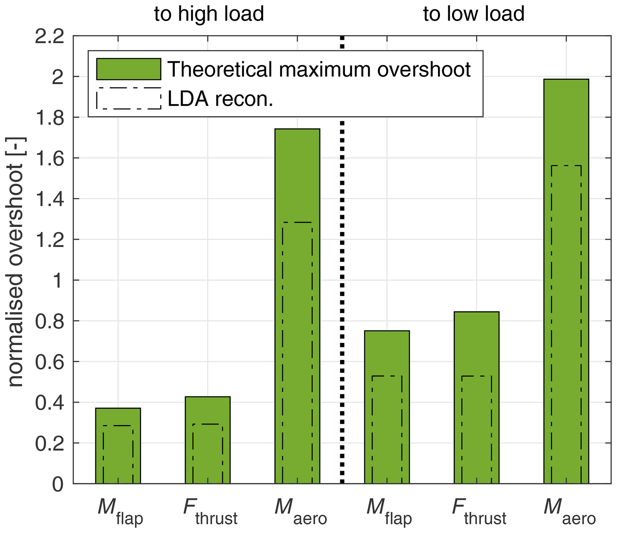
Figure 22Theoretical dynamic overshoot for the step to high and low loads for the integral turbine loads Mflap, Fthrust and Maero, based on reconstruction from the LDA data, assuming an infinitely fast pitch step in comparison to the LDA recon. case from Fig. 21a.
A clear difference can be seen between the pitch directions for the axial loads Mflap and Fthrust, with about twice as high an amount of overshoot for the step to low load than for the step to high load. For the torque, the general trend is the same with 2.5 to 4.5 times the overshoot in comparison to the other signals. The trend is similar to the repeated LDA recon. values in the plot.
In this section, the results for the inductions, wake flow and loads will be discussed. A focus for comparisons is on publications in connection to the NREL unsteady aerodynamics experiments phase VI (see Hand et al., 2001), later referred to as just phase VI, as this experiment is the most widely studied dynamic inflow dataset so far.
4.1 Induction transients
Dynamic inflow phenomena on wind turbines were already indirectly shown in experiments based on integral loads for the 2 MW Tjæreborg turbine (see Øye, 1991), based on pressure-sensor-derived sectional forces on the phase VI (see Hand et al., 2001) and MEXICO (see Boorsma et al., 2018) model turbines and in the wake measurements behind an actuator disc with dynamic thrust changes (see Yu et al., 2017). The presented axial induction transients in Fig. 9 based on the LDA measurements in the rotor plane are the first direct experimental evidence of dynamic inflow phenomena for wind turbines.
Pitch steps of the phase VI experiment were performed at 5 m s−1 wind speed and a tip speed ratio (TSR) of 7.5. The pitch step of 15.9∘ took place during approximately rotor revolution (pitch rate of 57∘ s−1 over 0.28 s). This extreme pitch step is between a very highly loaded rotor at a rotor equivalent axial induction of 0.5 and 0 for the unloaded rotor. At the highly loaded rotor state, the turbine is in the turbulent wake state. This high induction state was later suspected to be responsible for problems in validation (Sørensen and Madsen, 2006).
Pitch steps in this paper were performed at 6.1 m s−1 and a TSR of 7.4. The pitch step of 5.9° was performed during approximately rotor revolution between rotor equivalent inductions of 0.34 and 0.14. The experiment thus is not operated in the turbulent wake state at the high load case.
The observed slight radial dependency for the single time constant (see Fig. 10), where the values slightly decrease towards the tip for the step to low load is in accordance with the observation by Schepers (2007) for the phase VI experiment, despite the more extreme change in rotor loading.
Pirrung and Madsen (2018) reproduced this behaviour for the phase VI experiment in a cylindrical wake model simulation. They explain this observation by the nature of the dynamic inflow process that cannot be described correctly by a one-time-constant model but by a two-time-constant model. They reason that the axial induction adapts by different amounts during the pitch step depending on pitch direction. This is governed by the wake velocity before the pitch step and thus influences the one time constant fit to the normal forces after the overshoot. In contrast, in the presented axial induction transients (see Fig. 9), it is seen that it adapts similarly during the pitch step for both pitch directions, by 28 % on average.
For the two time-constant model fits to the axial wake inductions, two variants of time constants, one with a freely fitted weighting ratio kfree and one with a prescribed weighting ratio kfix, are shown in Fig. 11. Using kfix allows for a direct comparison of τfast and τslow between the pitch directions. The radial dependency of τfast, with high values towards the root, extends further into the blade for the step to low load. In their investigation of the normal force measurements on the phase VI experiment, Sørensen and Madsen (2006) also saw this high τfast values at the root nearest radius of 0.3 R for the step to low load but not for the step to high load. In the present and the phase VI experiment, this high τfast near the root is of the order of τslow. In the present experiment, there is a difference in the τfast between pitch directions, with lower values for the step to low load from 0.5 R to the tip. This difference between the pitch directions is not seen by Sørensen and Madsen (2006). Furthermore a radial dependance can also be seen from the middle of the blade towards the tip with an increase for the step to high load (67 %) and a slight decrease for the step to low load (−14 %).
For τslow, a very slight radial dependency can be seen for the fit with kfix, with slightly increasing values (11 %) towards the tip for the step to high load and slightly decreasing values (−16 %) for the step to low load, similar to the fit of τsingle.
The τslow values are on average about 28 % faster for the step to low load than for the step to high load. The same trend can be seen in Sørensen and Madsen (2006) but by a much higher value of around 100 %. The likely explanation is the higher difference in axial induction between the steady load levels for the phase VI experiment. Sørensen and Madsen (2006) and Pirrung and Madsen (2018) discuss this scaling of the time constants with the wake deficit and thus mean axial induction of the rotor. Also, the Øye dynamic inflow model (see Schepers and Snel, 1995) and other recent dynamic inflow models (e.g. Madsen et al., 2020) use the axial induction to scale the time constants. There the fast time constant represents the near-wake dynamics and decreases with radius and the slow time constant represents the far-wake dynamics.
Sørensen and Madsen (2006) and Pirrung and Madsen (2018) elaborated, based on measurements and simulations, that a two-time-constant model better describes the dynamic inflow process than a one-time-constant model. The two time constant approach also was implemented in the Øye dynamic inflow model (see Schepers and Snel, 1995). Yu et al. (2019) further showed, based on actuator disc vortex models, that a two-time-constant model describes the process better than a one or three-time-constant model. Comparing the fitting error of the 1c and 2c models to the axial wake induction measurements of the present experiment (see Fig. 12), this finding is verified based on the first direct measurements of dynamic inflow phenomena. However, the root region is an exception, as the process is defined by only one time constant.
The only minor differences in fitting error between the two variants with kfree and kfix (see Fig. 11) illustrate the high sensitivity of the fitting process. Small changes in k have a noticeable impact on the τfast and τslow values, where one increases as the other decreases.
The overshooting behaviour of the tangential induction is a new finding. The time constants of the one-time-constant model have no clear radial dependency. They are lower for the step to low load and in general, slightly lower than those fitted for the axial induction. The overshoot also is more prominent for the step to low load. This behaviour is of interest for the physical understanding of the dynamic inflow effect, as the overshoot in the torque is directly counteracted by the change in wake rotation. We assume that the shed vortices due to the change in circulation introduce this instant overshoot in tangential induction. For the modelling of the dynamic inflow effect in BEM-based codes, this behaviour is only of secondary interest, as the influence of the tangential induction on the angle of attack is negligible, apart from the blade root.
4.2 Wake evolution
No relevant influence of the shear layer between the open jet wind tunnel and the surrounding air is seen in the wake snapshots (see Fig. 15). On that basis, it was decided to include these measurements in the paper. The main near-wake and beginning far-wake dynamics due to the pitch step should not be disturbed, despite the high blockage ratio of 0.28, as long as the wake and the shear layer of the open jet wind tunnel flow do not interact.
The velocity snapshots in the wake show differences in wake evolution between the pitch directions. The faster progression of the wake for the pitch step to low load supports the presumption made by Schepers (2007) of different convection velocities of the wake consisting of the old vorticity and new vorticity, depending on the pitch direction. We assume the faster convection of this mixed wake for the case of the step to low load, starting with a low wake velocity pushed by a higher wake velocity to be the main driver of the faster time constants (τsingle and τslow) of the axial wake induction.
The dynamic widening of the wake after the pitch step to low load, as drawn in Fig. 15, is a new finding. We attribute it to the sudden change in trailed vorticity shed from the blade tip region. Part of the slow old wake is then pushed outboard by the fast new wake. The wake is not accelerated by the fast new wake at these larger radii but by the even faster free stream wind velocity. This behaviour is a possible explanation for the decreasing time constants τsingle, also τslow, towards the tip for the pitch step to low load.
The overshoot in the velocity in the wake after a sudden change in thrust, as observed here for the radii at 1.0 R for the step to high load (see Fig. 17), has been discussed by Yu et al. (2017) based on wind tunnel experiments with a variable porosity actuator disc. They attribute these overshoots to the shed vorticity at the actuator disc edge due to the fast thrust change. The local structure at 0.2 R, where the root transition towards the axis of rotation starts, is opposite to the overshoot at 1 R for the step to high load. We assume this to be the counterpart, the shed vorticity at the blade root, due to the sudden change in trailed vorticity. A connection of this shed root vortex to the radial dependency of τfast near the root cannot be concluded from the data but seems possible.
The quantitative comparison of the wake front velocity (see Fig. 18), as a measure of the convection of the transition point between old and new wake, shows the faster velocity for the step to low load. On average, this wake convection velocity is 26 % faster for the step to low load than for the step to high load. This difference resembles the difference in τsingle and τslow from the induction investigation in Sect. 4.1.
A fast initial wake front velocity is seen between 0.5 and 0.75 D, which is near the free stream velocity and higher for both cases than the expected axial wind velocity in the rotor plane for the low loaded rotor. An obvious explanation is that in the near wake, the dynamic inflow process of the whole rotor is governed by the influence of the trailed tip vortex, which does convect at similar velocities.
In the further course, the wake front velocity slows down for both cases. For the step to low load, it even slows down between 1.25 and 1.75 D to a lower value than the far-wake velocity according to momentum theory for the new steady state. This behaviour can be explained by the mixed wake of both the old and new wake, which influence each other.
4.3 Load transients
The general comparison of the load signals obtained from strain gauges and reconstructed from the LDA measurements (see Fig. 19) shows a good agreement and thus proved the physical consistency of the induction measurements for these dynamic experimental cases.
For the steady equilibrium, the comparison between the strain gauge measurements and the reconstructed loads (see Fig. 20) yields in generally good agreement, apart from the thrust at low load. Especially the here relevant high angle of attack region for the root airfoil is suspected to have uncertainties related to the low Reynolds number and possible laminar separation bubbles that can significantly increase the local lift.
For the flapwise blade root bending moment and the thrust, the load overshoot is much more pronounced for the step to low load than for the step to high load, whereas the trend for the torque is the same but to a smaller extent. The magnitude of the overshoot depends on how much the axial induction has already adapted during the pitch process. As discussed in Sect. 4.1, they adapt a similar amount during the pitch step for both pitch directions, so this cannot explain the difference in overshoot between the pitch directions. The more pronounced overshoot of loads is also discussed for the phase VI measurements in Schepers (2007). He suspected the high angles in the stall region at the highly loaded rotor blade to be a possible reason for that phenomenon. In contrast, the high load case is operating safe outside of the stall regime for the experiment presented here, apart from the very root.
The higher relative overshoot of the torque by a factor of 3 to 4.5 compared to the flapwise blade root bending moment and the rotor thrust can be related to the lag in inflow angle and thus angle of attack behind the quasi-steady value. Mflap and Fthrust feel the effect mainly due to the change in the magnitude of the lift force, while Maero feels the change in magnitude and also the change of the projection of the lift force in the tangential direction due to the lag of the inflow angle (see Eq. 12). Because the Fthrust and mostly also Mflap are determined by the cosine of the inflow angle (see Eq. 11), the effect of the inflow angle lag is much smaller here.
The simplified approach to estimate the theoretical maximum overshoot for the load signals based on the steady inductions and the pitch angle change with the BET reconstruction (see Fig. 22), provides a solid reason for the different amount of load overshoot. It only depends on the turbine load characteristic, as the theoretical overshoot show a very similar ratio between load channels and pitch directions to the actual measured and reconstructed load overshoot. The angle of attack overshoot for both pitch directions is the same in this thought experiment; however, near the high load the turbine reaction is less sensitive to the angle of attack changes than at the low load state.
Further, in the overshoot analysis (see Fig. 21a) the large differences for the thrust between the strain gauge measurement and the reconstructed loads, both with and without the unsteady airfoil aerodynamics model, catches the eye. At closer investigation, the dynamic correction based on the estimated eigenfrequency and damping coefficient seems to be unsuited for very detailed comparisons. Therefore, this signal channel is omitted in the discussion of the detailed comparison. For the blade root bending moment and torque, the fit is good.
The 1c model investigation shows a good agreement between the strain-gauge-measurement-derived and reconstruction-based τsingle values. They are larger for the step to high load than for the step to low load, which is consistent with what was found before in the analysis of induction and wake results. They have a similar size to the fitted time constants to the axial inductions. The small changes in the overshoot of the reconstructed loads the uA model introduces demonstrate the sensitivity of the time constant fits to these small changes in the signal.
Structural interactions are assumed to be the main driver for the observed differences in overshoot and also for the differences in the fitted time constants between the strain gauge signals and reconstructed loads with and without the uA model.
The objective of the presented dynamic inflow measurements was to deepen the general physical understanding of the dynamic inflow effect for wind turbines.
Direct experimental evidence of dynamic inflow is given through a very clear delay of induction factors at different radial positions at the rotor plane in response to a pitch angle step. Until now, dynamic inflow effects were only proven indirectly through measurements of turbine loads or flow measurements in the wake. It is affirmed that a two-time-constant model is more suited than a one-time-constant model to describe the behaviour of the axial induction for such a pitch step. The fast time constant of this model, representing the near-wake influence, has a strong radial dependency near the root and a clear, respectively slight, dependency in the middle and tip region for the step to high, respectively low, load. The slow time constant, related to the close far wake, shows a slight decrease towards the outer part for the step to low load and a slight increase for the step to high load. The overshooting behaviour of the tangential induction is a novel finding of this work. It could be explained by the shed vorticity, which results from the circulation change during the pitch step. We expect that the radial dependency of the axial induction time constant is related to the observed dynamic wake expansion for the step to low load. With the wake measurement, it is affirmed that the formation of the mixed wake after the pitch step convects faster for the step to low load, than for the step to high load. We suppose that this is the reason for the lower slow time constants of the axial induction for the step to low load. It is found that the mixed wake after the pitch step initially travels at nearly free stream velocity for both pitch directions. We assume that the dynamic inflow effect in this near wake is governed by the tip vortex due to the fast change in trailed vorticity. These vortices travel at such high velocities. Another finding is that the initial decay of the axial inductions during the pitch step is similar for both pitch directions. Furthermore, the aerodynamic characteristics of the turbine is identified to be the reason for the higher load overshoot for the pitch step to low load.
This comprehensive pitch step measurement set allows for detailed validation of engineering models and simulations for two relevant operational states, as we performed with the induction data in Berger et al. (2020).
Further investigations are recommended with high-fidelity models of induction effects, e.g. FVWM or actuator line CFD simulations, to support the interpretation of the data and improvement of models. Further planned steps to extend the understanding of the dynamic inflow process and enhance or develop models on the basis of this experimental setup are the generation of a wider database of pitch steps with varying parameters of inflow velocities, rotor speeds and rotor induction levels but also more realistic inflow conditions, including e.g. non-uniform inflow and gusts. With a wider database it can be tested whether, besides the axial induction, radial position and typical dynamic inflow time scaling factor have a significant influence on the time constants, as, for example, the operating TSR, background turbulence or non-uniform inflow. Due to the scaling of induction aerodynamics of this model turbine, based on the NREL 5 MW turbine, the general behaviour of the induced velocities and wake are very similar to that turbine. It thus enables non-dimensional comparisons with that reference turbine, a turbine that has been extensively used worldwide in validation studies.
The detailed derivation based on the theorem of Biot–Savart is given in Herráez et al. (2018), but the relevant formulas to produce the analytical solution in Fig. 5a are given here.
Equation (A11) of Herráez et al. (2018) is reproduced in Eq. (A1). The velocity induced by each of the N rotor blades (numbered i∈[1, 2, …, N]) is given as a function of the azimuth angle of the blade ψi, the azimuth angle of the sampling point β and the coordinates along the blade spanwise direction l. The circulation along the blade span is given by Γi(l) and the azimuth angle of all blades can be defined by , where .
Herráez et al. (2018) use a phase lock of the rotor for the simulations and compute the velocity along a circle for a specific radius. For the PIV validation in Herráez et al. (2018) and the application in this paper, a stationary probe is used and the rotor position is varied. The circulation Γi(l) is obtained from the lift distribution calculated in Eq. (9) by the Kutta–Joukowski theorem.
The analytical solution of the axial probe uprobe, analytical in Fig. 5a considers an axial velocity of uax=4 m s−1 and the combined effect of all three blades according to Eq. (A2). Note that Eq. (A1) has a singularity for the probe position and a blade element being at the exact same position that are excluded from the plot (90, 210 and 330∘).
The uA model as described in detail in Pirrung et al. (2017) Sect. 2.3 is reproduced with slightly altered variable names.
The model consists of two filter functions, Eqs. (B2) and (B3), which use the same time constant , defined in Eq. (B1). The index j denotes the time step, and the index QS the quasi-steady solution. The time step of the simulation, thus reconstruction, is defined by Δt. The effective angle of attack , which includes the uA effect, is obtained by Eq. (B4).
The 1c model fit is applied to the hot-wire signal shown in Fig. 17. The fit does start at t0, which is defined at the point where the velocity has adjusted by 28 % to the new equilibrium. This definition is less accurate than the end of the pitch step, as for the axial induction transients. However, no direct fitting start time can be defined and this value is based on the mean value the axial inductions have adjusted during the pitch step. The aim of this definition is to make the time constants comparable to these time constants of the axial wake induction.
Further, the fitted τsingle values for the wake flow measurements are comparable for both pitch directions. They are presented in Fig. C1.
Between 0.5 and 1.5 D no clear differences can be seen between pitch directions, apart from the root nearest radius of 0.2 R. The fitting of this radius is very sensitive due to the described local structure within the signal and should not be overinterpreted. For farther distances behind the turbine at 1.75 and 2 D, there is a clear difference between the pitch directions, with noticeable higher time constants for the step to high load for the radial range of 0.4 to 1 R, compared to both the time constants for the step in the same direction at rotor nearer distances and also in comparison to the step to low load at the same distances.
In the actuator disc experiments by Yu et al. (2017), this trend also seems to be more prominent for the higher distances from the actuator disc.
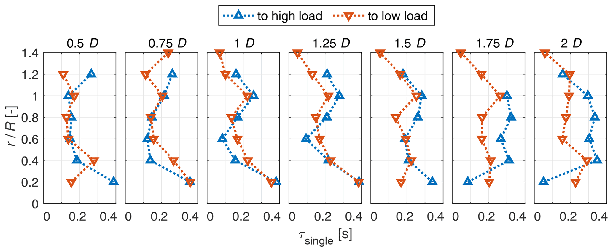
Figure C1Spanwise evolvement of the axial wake velocity from 0.5 to 2 D parameterised by the fitted time constant of the one-time-constant model for both pitch directions.
The preprocessed experimental data along with further documentation are available at https://doi.org/10.5281/zenodo.5552171 (Berger et al., 2021). We encourage researchers to use the data for validation purposes or any other scientific use.
FB designed, performed, processed and analysed the experiment and wrote the article. DO assisted in the experiment, estimated steady corrections and wrote postprocessing scripts for the LDA data. JGS and MK contributed with several fruitful discussions from an early planning stage. MK supervised the work. All co-authors thoroughly reviewed the article.
The contact author has declared that neither they nor their co-authors have any competing interests.
Publisher's note: Copernicus Publications remains neutral with regard to jurisdictional claims in published maps and institutional affiliations.
We thank Iván Herráez and Elia Daniele for the discussions on the wake induction measurement method. We further thank Dominik Traphan and Tom Wester for their help with the LDA system. We would also like to thank the two reviewers Luca Greco and Georg Raimund Pirrung for their helpful comments.
This work was partially funded by the Ministry for Science and Culture of Lower Saxony through the funding initiative Niedersächsisches Vorab in the project “ventus efficiens” (reference no. ZN3024).
This paper was edited by Alessandro Bianchini and reviewed by Georg Raimund Pirrung and Luca Greco.
Berger, F. and Kühn, M.: Experimental investigation of dynamic inflow effects with a scaled wind turbine in a controlled wind tunnel environment, J. Phys.: Conf. Ser., 1037, 052017, https://doi.org/10.1088/1742-6596/1037/5/052017, 2018. a
Berger, F., Kröger, L., Onnen, D., Petrović, V., and Kühn, M.: Scaled wind turbine setup in a turbulent wind tunnel, J. Phys.: Conf. Ser., 1104, 012026, https://doi.org/10.1088/1742-6596/1104/1/012026, 2018. a
Berger, F., Höning, L., Herráez, I., and Kühn, M.: Comparison of a radially resolved dynamic inflow pitch step experiment to mid-fidelity simulations and BEM, J. Phys.: Conf. Ser., 1618, 052055, https://doi.org/10.1088/1742-6596/1618/5/052055, 2020. a
Berger, F., Onnen, D., Schepers, J, G., and Kühn, M.: Dataset – Radially resolved dynamic inflow pitch step experiment in wind tunnel, Zenodo [data set], https://doi.org/10.5281/zenodo.5552171, 2021. a
Boorsma, K., Schepers, J. G., Gomez-Iradi, S., Herraez, I., Lutz, T., Weihing, P., Oggiano, L., Pirrung, G., Madsen, H. A., Rahimi, H., and Schaffarczyk, P.: Final report of IEA Task 29, Mexnext (Phase 3), Tech. Rep. ECN-E–18-003, Energy research Center of the Netherlands, Petten, 2018. a, b
Drela, M.: XFoil: An Analysis and Design System for Low Reynolds Number Airfoils, in: Lecture Notes in Engineering, vol. 54, Springer, Berlin, Heidelberg, 1989. a
Ferreira, C., Yu, W., Sala, A., and Vire, A.: Dynamic inflow model for a Floating Horizontal Axis Wind Turbine in surge motion, Wind Energ. Sci. Discuss. [preprint], https://doi.org/10.5194/wes-2021-34, in review, 2021. a
Hand, M. M., Simms, D. A., Fingersh, L. J., Jager, D. W., Cotrell, J. R., Schreck, S., and Larwood, S. M.: Unsteady Aerodynamics Experiment Phase VI: Wind Tunnel Test Configurations and Available Data Campaigns, Tech. Rep. NREL/TP–500–29955, National Renewable Energy Laboratory, Golden, 2001. a, b, c
Hansen, M. H., Gaunaa, M., and Madsen, H. A.: A Beddoes-Leishman type dynamic stall model in state-space and indicial formulations, Tech. Rep. Risø-R-1354(EN), Forsnikscenter Risø, Risø, 2004. a
Hansen, M. O. L.: Aerodynamics of Wind Turbines, Earthscan, London, 2008. a
Herráez, I., Daniele, E., and Schepers, J. G.: Extraction of the wake induction and angle of attack on rotating wind turbine blades from PIV and CFD results, Wind Energ. Sci., 3, 1–9, https://doi.org/10.5194/wes-3-1-2018, 2018. a, b, c, d, e, f, g, h, i
Jonkman, J., Butterfield, S., Musial, W., and Scott, G.: Definition of a 5-MW Reference Wind Turbine for Offshore System Development, Tech. Rep. NREL/TP-500-38060, National Renewable Energy Laboratory, Golden, 2009. a
Kröger, L., Frederik, J., Van Wingerden, J. W., Peinke, J., and Hölling, M.: Generation of user defined turbulent inflow conditions by an active grid for validation experiments, J. Phys.: Conf. Ser., 1037, 052002, https://doi.org/10.1088/1742-6596/1037/5/052002, 2018. a
Madsen, H. A., Larsen, T. J., Pirrung, G. R., Li, A., and Zahle, F.: Implementation of the blade element momentum model on a polar grid and its aeroelastic load impact, Wind Energ. Sci., 5, 1–27, https://doi.org/10.5194/wes-5-1-2020, 2020. a, b, c
Medici, D., Ivanell, S., Dahlberg, J.-Å., and Alfredsson, P. H.: The upstream flow of a wind turbine: blockage effect, Wind Energy, 14, 691–697, https://doi.org/10.1002/we.451, 2011. a
Øye, S.: Tjæreborg Wind Turbine: 4. dynamic inflow measurement. Lyngby, Tech. rep. VK-204, Department of Fluid Mechanics, Technical University of Denmark, Lyngby, 1991. a, b
Pirrung, G., Riziotis, V., Madsen, H., Hansen, M., and Kim, T.: Comparison of a coupled near- and far-wake model with a free-wake vortex code, Wind Energ. Sci., 2, 15–33, https://doi.org/10.5194/wes-2-15-2017, 2017. a, b
Pirrung, G. R. and Madsen, H. A.: Dynamic inflow effects in measurements and high-fidelity computations, Wind Energ. Sci., 3, 545–551, https://doi.org/10.5194/wes-3-545-2018, 2018. a, b, c, d
Rahimi, H., Schepers, J. G., Shen, W. Z., García, N. R., Schneider, M. S., Micallef, D., Ferreira, C. J., Jost, E., Klein, L., and Herráez, I.: Evaluation of different methods for determining the angle of attack on wind turbine blades with CFD results under axial inflow conditions, Renew. Energy, 125, 866–876, https://doi.org/10.1016/j.renene.2018.03.018, 2018. a
Ryi, J., Rhee, W., Chang Hwang, U., and Choi, J.-S.: Blockage effect correction for a scaled wind turbine rotor by using wind tunnel test data, Renew. Energy, 79, 227–235, https://doi.org/10.1016/j.renene.2014.11.057, 2015. a
Schepers, J. and Snel, H.: Dynamic inflow: yawed conditions and partial span pitch control, Tech. Rep. ECN-C–95-056, Energy research Center of the Netherlands, Petten, 1995. a, b, c, d
Schepers, J. G.: IEA Annex XX: Dynamic Inflow effects at fast pitching steps on a wind turbine placed in the NASA-Ames wind tunnel, Tech. Rep. ECN-E–07-085, Energy research Center of the Netherlands, Petten, 2007. a, b, c, d
Schepers, J. G.: Engineering models in wind energy aerodynamics: Development, implementation and analysis using dedicated aerodynamic measurements, PhD thesis, TU Delft, Delft, https://doi.org/10.4233/uuid:92123c07-cc12-4945-973f-103bd744ec87, 2012. a, b
Schepers, J. G. and Schreck, S. J.: Aerodynamic measurements on wind turbines, Wiley Interdisciplin. Rev.: Energ. Environ., 8, e320, https://doi.org/10.1002/wene.320, 2018. a, b
Shen, W. Z., Mikkelsen, R., Sørensen, J. N., and Bak, C.: Tip loss corrections for wind turbine computations, Wind Energy, 8, 457–475, https://doi.org/10.1002/we.153, 2005. a
Snel, H. and Schepers, J.: Joint investigation of dynamic inflow effects and implementation of an engineering method, Tech. Rep. ECN-C–94-107, Energy research Center of the Netherlands, Petten, 1995. a, b
Snel, H., Houwink, R., Bosschers, J., Piers, W. J., van Bussel, G., and Bruining, A.: Sectional prediction of 3-D effects for stalled flow on rotating blades and comparison with measurements, Tech. Rep. ECN-RX–93-028, Energy research Center of the Netherlands, Petten, 1993. a
Sørensen, N. N. and Madsen, H. A.: Modelling of transient wind turbine loads during pitch motion, in: vol. 1, EWEC 2006, 786–795, 2006. a, b, c, d, e, f, g, h
van Engelen, T. G. and Hooft, E. L. V. D.: Dynamic inflow compensation for pitch controlled wind turbines, Tech. Rep. ECN-RX–04-129, Energy research Center of the Netherlands, Petten, 2004. a
Vermeer, L., Sørensen, J., and Crespo, a.: Wind turbine wake aerodynamics, Progr. Aerosp. Sci., 39, 467–510, https://doi.org/10.1016/S0376-0421(03)00078-2, 2003. a
Yu, W., Hong, V. W., Ferreira, C., and van Kuik, G. A. M.: Experimental analysis on the dynamic wake of an actuator disc undergoing transient loads, Exp. Fluids, 58, 149, https://doi.org/10.1007/s00348-017-2432-9, 2017. a, b, c, d
Yu, W., Tavernier, D., Ferreira, C., van Kuik, G. A., and Schepers, G.: New dynamic-inflow engineering models based on linear and nonlinear actuator disc vortex models, Wind Energy, 22, 1433–1450, https://doi.org/10.1002/we.2380, 2019. a, b
- Abstract
- Introduction
- Methods
- Results
- Discussion
- Conclusions
- Appendix A: Counterbalance of the blade induction at the bisectrix between consecutive blades
- Appendix B: Unsteady aerodynamics model
- Appendix C: Time constant analysis of wake
- Data availability
- Author contributions
- Competing interests
- Disclaimer
- Acknowledgements
- Financial support
- Review statement
- References