the Creative Commons Attribution 4.0 License.
the Creative Commons Attribution 4.0 License.
 | 05 Jan 2021
Constructing fast and representative analytical models of wind turbine main bearings
James Stirling
Edward Hart
Abbas Kazemi Amiri
This paper considers the modelling of wind turbine main bearings using analytical models. The validity of simplified analytical representations used in existing work is explored by comparing main-bearing force reactions with those obtained from higher-fidelity 3D finite-element models. Results indicate that there is good agreement between the analytical and 3D models in the case of a non-moment-reacting support (such as for double-row spherical roller bearings), but the same does not hold in the moment-reacting case (such as for double-row tapered roller bearings). Therefore, a new analytical model is developed in which moment reactions at the main bearing are captured through the addition of torsional springs. This latter model is shown to significantly improve the agreement between analytical and 3D models in the moment-reacting case. The new analytical model is then used to investigate load characteristics, in terms of forces and moments, for this type of main bearing across different operating points and wind conditions.
- Article
(3028 KB) - Full-text XML
- BibTeX
- EndNote


Wind energy provides an important and growing contribution to the European energy market, with 205 GW installed as of 2019 – accounting for 15 % of consumed electricity (Wind Europe, 2020). As part of this growth, more wind farms are being planned and constructed offshore to take advantage of higher wind speeds and more available construction space (Junginger et al., 2004). Recent trends show dramatic falls in the cost of offshore wind, as has been mirrored in the UK's contract for difference auctions, which have seen prices drop to GBP 57.50 MWh−1 (UK Government, 2017) and even lower.
With turbines moving further offshore and a need to bring costs down, reducing operation and maintenance costs, which can be as high as 35 % of the total lifetime costs of a project, is becoming increasingly important for wind farm operators (Sinha and Steel, 2015). This in turn effects technology design and selection and puts pressure on original equipment manufacturers (OEMs) and operators to improve turbine reliability. As such, reliability and failure rate considerations have received much attention in the literature (Tavner et al., 2007; Wilkinson, 2011; Artigao et al., 2018).
One turbine component with relatively high failure rates and associated downtime is the main bearing (MB). MBs are becoming recognised as an important component for which failures need to be better understood and reliability improved (Keller et al., 2016; Hart et al., 2020). MB failure rates have been reported as being as high as 30 % (Hart et al., 2019) across a 20-year lifetime, with some wind farms having reported MBs failing in less than 6 years (Sethuraman et al., 2015). Recent work which has demonstrated important and unusual load behaviours in wind turbine MBs (Hart et al., 2019; Hart, 2020) implements simplified analytical representations of the drivetrain. Such representations are necessary if this type of analysis is to be performed across large numbers of load cases, incorporated into fleet-wide modelling, or into industry standard simulation software (e.g. Bladed and Fast). These types of analytical models are therefore important and already being utilised, and, as such, a detailed assessment of how effectively they represent wind turbine drivetrain load response at the MB for different bearing types is an important next step in their development.
Wind turbine drivetrains and MBs in particular are specific to individual turbine designs. As such, it is beneficial to understand in as much generality as possible how existing simple representations may be used to study MB load response without focusing on any design case (since this would reduce the generality of results). In order to move in this direction, it is necessary to work through levels of modelling complexity, understanding at each stage how well a given model represents the next in the chain. This approach also develops knowledge about which effects can be adequately captured at a given level of model complexity, helping inform decisions with respect to model selection for specific applications.
This paper considers an important step in the overall modelling chain starting with existing 2D, orthogonally independent, simply supported models and looking to compare with higher-fidelity models which are closer to representing real-world wind turbine MBs. The strongest assumptions in the existing models are independence of horizontal and vertical planes (from a load perspective) and simply supported load reactions (i.e. the bearing does not support moment loads). Therefore, this work seeks to compare their performance with more realistic models that remove one or both of these assumptions. More explicitly, 3D finite-element (FE) modelling removes the 2D and orthogonality assumptions. With respect to simple versus other supports, MBs for wind turbines have two “types” of reaction behaviour in general: those that support forces only and not moments (e.g. double-row spherical roller bearings, DSRBs) and those that support both forces and moments (e.g. double-row tapered roller bearings, DTRBs). Three-dimensional FE models which have reaction behaviours that emulate each of the two types are therefore considered. Hence, the overarching goal of this paper is to explore the following question: can analytical models be used to effectively evaluate load reactions for three-dimensional main-bearing support configurations with either moment-reacting or non-moment-reacting behaviours?
Section 2 summarises previous work undertaken in this area. Section 3 then introduces the higher-fidelity 3D models which are used to compare with analytical model outputs. Section 4 presents the results of the comparison, with Sect. 5 then extending the analytical model to include moment reactions at the MB. In Sect. 6 the new analytical model is used to study load behaviours for this bearing type. Finally, Sect. 7 discusses some practicalities surrounding the application of these models before Sect. 8 presents the conclusions of this work.
Despite having received less attention than other drivetrain components, there have been a number of high-quality research papers which include modelling and analysis of wind turbine MBs. Cardaun et al. (2019) use a multibody simulation model with flexible components in SIMPACK to investigate main-bearing loads for a yawed turbine. It was found that yawed inflow has an asymmetric effect on main-bearing loading and fatigue, with the possibility of either increasing or decreasing loading and load fluctuations depending on yaw direction relative to inflow. Bosmans et al. (2019) represent the drivetrain system as lumped parameter components. In order to keep degrees of freedom low and increase the speed of simulations, bearings are modelled as linear springs. The study showed differences between port-based and 1D–3D nesting models. In this study focus is on the intermediate- and high-speed shafts, and so the MB is not discussed in detail. In Wang et al. (2020b) the MB is modelled within an overall numerical model of the drivetrain using SIMPACK software. The model consists of both rigid and flexible bodies, with bearings modelled as force elements with linear force–deflection relationships. High-fidelity FE models of the critical components are developed in ANSYS before modal reduction is used to minimise degrees of freedom for reduced FE bodies in the system. The paper sought to determine 20-year drivetrain fatigue damage and found that the highest fatigue damage is experienced by the upwind MB. Wang et al. (2020a) determine MB loading for the case where a flexible bedplate is included in modelling. Effects on damage-equivalent fatigue loads are explored for flexible and rigid bedplate cases. The study concludes that flexibility in the bedplate leads to a reduction in loading and fatigue experienced by MBs when compared to the rigid case. Kock et al. (2019) use high-fidelity FE models to investigate MB internal load distributions and contact pressures when considering variations in elasticity about the bearing circumference and clearance values. Their findings indicate that bearing housing elasticity strongly influences the number of rolling elements under load and the maximum forces experienced by rolling elements.
In addition to the analyses outlined above, work has also been undertaken in which simple drivetrain representations are used to study general characteristics of MB loads and their relationship to the incident wind field (Hart et al., 2019; Hart, 2020), with the current paper building directly on these. The first of these (Hart et al., 2019) considered load characteristics for different possible drivetrain configurations and demonstrated sensitivities to both wind field characteristics and drivetrain set-up. More recently, work was undertaken in which repeating structures in time-varying MB loading were identified and characterised, with impacts on the loading experienced by bearing rolling elements also studied. As touched upon in Sect. 1, the benefit of analytical models employed previously is their simplicity and speed, allowing large numbers of load cases to be analysed rapidly in order to seek possible identifiable trends or recurring off-design load events which may require more detailed scrutiny. While practical for such analyses, it is important to consider the accuracy of these models given their inherent simplifying assumptions and the existence of different load reaction behaviours for different bearing types. These accuracy considerations form the focus of the current paper. The single-MB model and turbulent wind field simulations from Hart et al. (2019) are used here. As such, both are described below in more detail.
Hart et al. (2019) performed a MB load analysis using simulated loading in realistic wind fields. The three-dimensional turbulent wind fields were generated in Bladed software using a Kaimal spectrum to describe the second-order wind field statistics. The three parameters which characterise these wind fields are hub-height mean wind speeds (10, 12, 16, 20 m s−1), turbulence intensity (TI) (low, medium, and high, as specified by the IEC, 2005), and shear profile (power law shear exponents of 0.2 and 0.6). Six different wind fields were generated for each combination of these second-order statistics using different initial random number seeds as required for design certification (IEC, 2005). The above provides a total number of 144 realistic 3D turbulent wind fields spanning a significant range of typical operational conditions. The six wind fields associated with each combination of the parameters are referred to as common parameter load sets (CPLS). A 2 MW wind turbine was then simulated, operating in each of these 10 min wind fields using DNV GL Bladed aeroelastic software, with hub loading time series extracted. This resulted in 144 realistic 10 min hub loading time series for the 2 MW wind turbine, and it is these same load files which are used as inputs to models throughout the current paper. These hub loading time series were then applied to simplified models of MB set-ups (the one used in the current paper is outlined below) in order to study MB load characteristics. Drivetrain details were provided by Onyx Insight; this included gearbox connections represented as radial and axial linear springs. Three analytical models were defined, which included a single-main-bearing (SMB) system and two double-main-bearing (DMB) systems. The analytical model for the SMB drivetrain configuration is shown in Fig. 1, and this is the case considered here.
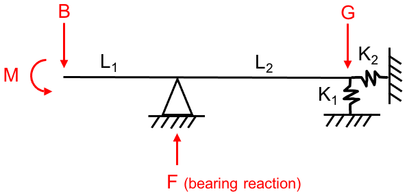
Figure 1Analytic model for single-main-bearing set-up in one plane. The full model consists of two such representations, one in each of the horizontal and vertical planes (Hart et al., 2019).
The equation system for the SMB drivetrain set-up is statically determinate and can be solved by balancing the moments about the gearbox, giving
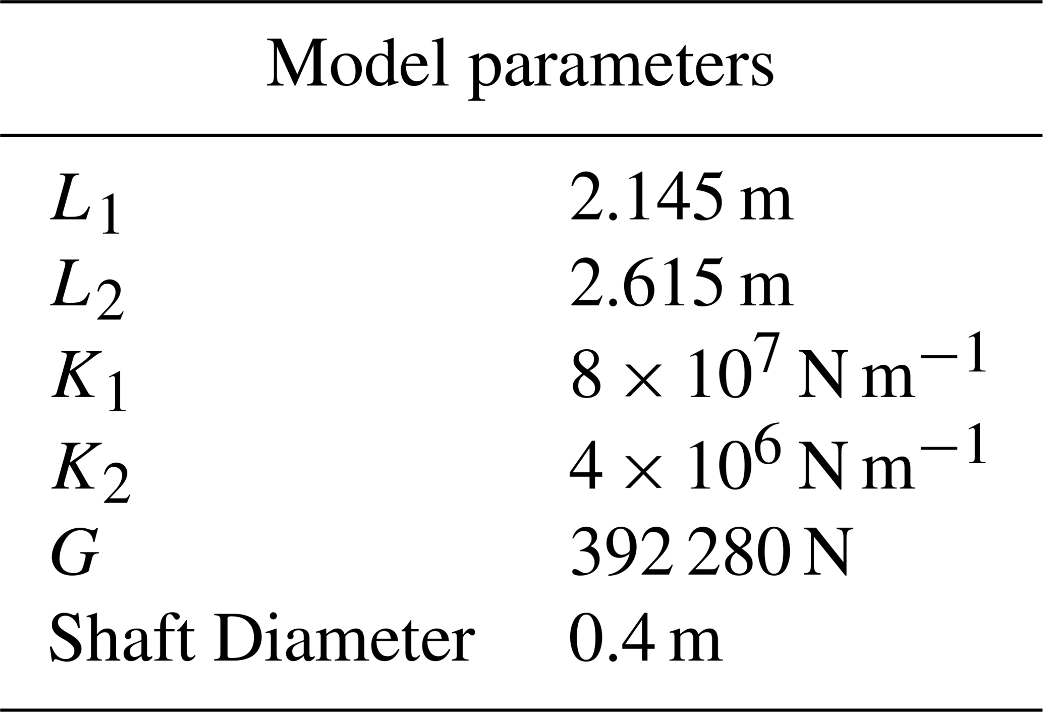
It is important to note that the overall model consists of two of the type shown in Fig. 1 – one in the horizontal and one in the vertical plane – with the resultant force being a vector combination of the two reaction forces at the MB. B and M represent force and moment loads at the hub, and L1 and L2 represent the distances between the hub and MB and between MB and gearbox, respectively. The axial and radial springs to the right of the model (K1 and K2) represent the connection between the shaft and gearbox as stiffness values, while G represents the gearbox weight in the vertical plane and is 0 in the horizontal plane. F is the main-bearing reaction force. All model parameters can be found in Table 1.
While models and results in Hart et al. (2019) demonstrate potentially important findings, the utilised models are simple and hence come with limitations. The bearings are modelled as single-point fixed supports, meaning all loading is reacted as forces at the MB, with no moment reactions present. The model also assumes the independence of loading and reaction behaviour in the horizontal and vertical planes. As outlined in Sect. 1, two common bearings used for wind turbine MBs are DSRBs, which cannot support moment loads, and DTRBs, which can support both forces and moments (Yagi, 2004; Smalley, 2015; Hart et al., 2020). Therefore, the validity of existing models when representing different bearing types and possible 3D effects is to be considered.
In order to assess the effectiveness of the simple analytical models used thus far, two FE models of the SMB system were created in ANSYS. The FE models were designed to be general and do not seek to represent any particular bearing specifically but rather the global behaviour of different bearing types: one designed to behave like a DSRB (non-moment-reacting) and the other to behave like a DTRB (does support moment loads). Likewise, the rest of the drivetrain system such as the shaft and gearbox connections remains both general and similar for the two different bearing types to create a like-for-like study. The models were subjected to the same hub loading as the analytical models outlined in the previous section, with bearing support reaction forces outputted and compared with those from the analytical model. Both FE models share dimensions with the SMB analytical model. The FE models themselves still remain relatively simple, with relevant behaviours captured without the modelling of individual rolling elements, as described below. To aid reproducibility, input and output value examples for all models are given in Table A1 of Appendix A.
3.1 DSRB FE model
The DSRB FE model was created with three separate bodies, referred to here as the shaft, the bearing, and the bearing housing (see Fig. 3a). The bearing was connected to the shaft using a bonded-type contact, and the convex outer face of the bearing was connected to the concave inner face of the bearing housing with a spherical joint. This type of connection allows the bearing housing to deformably react forces in the horizontal, vertical, and axial axes while being able to move freely in the rotational degrees of freedom, allowing the non-moment-reacting behaviour of a DSRB to be captured without the complex modelling of individual rollers. The full model is displayed in Fig. 2, and a sliced view of the bearing, housing, and shaft can be seen in Fig. 3a side-by-side with spherical-roller-bearing (SRB) elements overlaid on the same image to demonstrate the interface type being represented. Bearing clearance is assumed to be 0 since this parameter most directly influences the internal load distribution rather than overall reaction force. The bedplate is assumed to be rigid in this model, which, from previous work (Kock et al., 2019; Wang et al., 2020a), can be expected to provide conservatively higher bearing unit reaction force results than if bedplate flexibility were included.1 A fixed support was added to the base of the bearing housing to represent the connection to the bedplate, and the connection between the low-speed shaft and the gearbox was modelled by three body-to-ground spring connections in the horizontal, vertical, and axial directions. Appropriate equivalent stiffness values of the connections between the low-speed shaft and the gearbox were determined with the use of Romax Technology software. The stiffness values, along with model dimensions, can be found in Table 1. The shaft, along with the rest of the model, was designed to be general and is modelled as a solid piece of material. Actual wind turbine main shafts tend to be a mostly solid piece of material, although a small hole will run throughout the centre to allow for wiring to pass to the hub. A sensitivity analysis was therefore undertaken to determine the effect shaft thickness has on results; this can be found in Appendix B, and findings indicate low sensitivity to this value. A convergence study was undertaken to determine appropriate mesh densities, resulting in smaller elements on the bearing and housing bodies and larger elements on the shaft. Input hub loading was applied to the front face of the shaft, the gearbox weight was applied to the rear of the shaft in the vertical axis, and main-bearing reaction forces were extracted from the fixed support at the base of the housing.
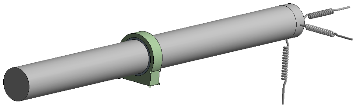
Figure 2The three-dimensional finite-element model with double-row spherical-roller-bearing-type reaction behaviour.

Figure 3(a) A split view of the SRB FE model displaying the geometries of the bearing and housing. (b) A split view of the TRB FE model displaying the geometries of the bearing and housing. Note: the roller elements and mesh displayed in these images are for illustrative purposes only; a finer mesh was used for the simulations.
3.2 DTRB FE model
The DTRB FE model was created with two separate bodies, referred to here as the shaft and the bearing–bearing housing (see Fig. 3b). The bearing–bearing housing was modelled as one piece of material and connected to the shaft using a bonded-type contact. This assumes 0 clearance between the rollers and housing (typically found in pre-loaded DTRBs) and allows the bearing unit to emulate the force and moment reaction properties of a DTRB. The dimensions of the model, assumptions of a rigid bedplate, and fixed-support connection from the base of the bearing–bearing housing to the bedplate are the same as those outlined above in the DSRB description. The low-speed-shaft-equivalent connection to the gearbox and applications of hub and gearbox loading are also the same as described above. The full model is displayed in Fig. 4, and a sliced view of the bearing–bearing housing and shaft can be seen in Fig. 3b side-by-side with tapered-roller-bearing (TRB) elements overlaid on the same image to demonstrate the interface type being represented. Model parameters can be found in Table 1. The shaft was again modelled as a solid piece of material. Sensitivity analysis results for this configuration, relating to shaft thickness, can also be found in Appendix B. A convergence study was again undertaken to determine appropriate mesh densities. The DTRB main-bearing reaction forces were extracted from the fixed support at the base of the housing.
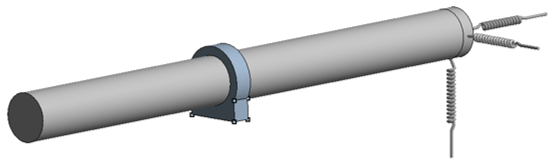
Figure 4The three-dimensional finite-element model with double-row tapered-roller-bearing-type reaction behaviour.
3.3 Bearing contact assumptions
Internal contact conditions and load distributions around the bearing circumference are important (and non-linear) aspects of bearing behaviour. However, the SMB analytical model being studied is not designed to go to this level of detail, instead outputting the reaction forces at (or equivalently the loads applied to) the MB. As such, the simplified FE representations for DSRB and DTRB bearings outlined above are considered reasonable for the following reasons: in the DSRB case, DSRBs are self-aligning and hence provide force but not moment reactions across the bearing, and as such, the reaction force required to balance the system should remain the same irrespective of the spring properties, with only displacement magnitudes effected, since the system is determinate; in the DTRB case, the system supports moments through opposite force reactions over the two bearing rows in addition to providing an overall force reaction. Consequently, non-linear contact properties of the rollers will influence the share between force and moment reactions at the MB. However, the non-linearity present in line contact rollers2 is only slight, with an exponent of 1.11 (Harris, 2006), and so they are reasonably approximated as linear (Dowson and Higginson, 1977; Tibbits, 2005). Considering the research question posed in Sect. 1, it is therefore argued that the FE DTRB model presented here sensibly recreates load reaction behaviours of the desired type.
The analytical model presented in Sect. 2 was compared with the FE models described in Sect. 3 to determine its validity when the 2D orthogonality and simply supported reaction assumptions are removed. The models were compared by performing a root mean squared error (RMSE) analysis between the reaction force results for the models across the whole range of turbulent wind field load time histories. Plots of RMSE between the analytical and two FE models are shown in Figs. 5 and 7, along with example time series plots of MB reaction forces in Figs. 6 and 8. The RMSE plots present the mean and standard deviations within each CPLS (which each capture results from six wind files with parameters in common) with respect to mean wind speed, turbulence intensity, and shear profile. Note that mean wind speed values are staggered for clarity.
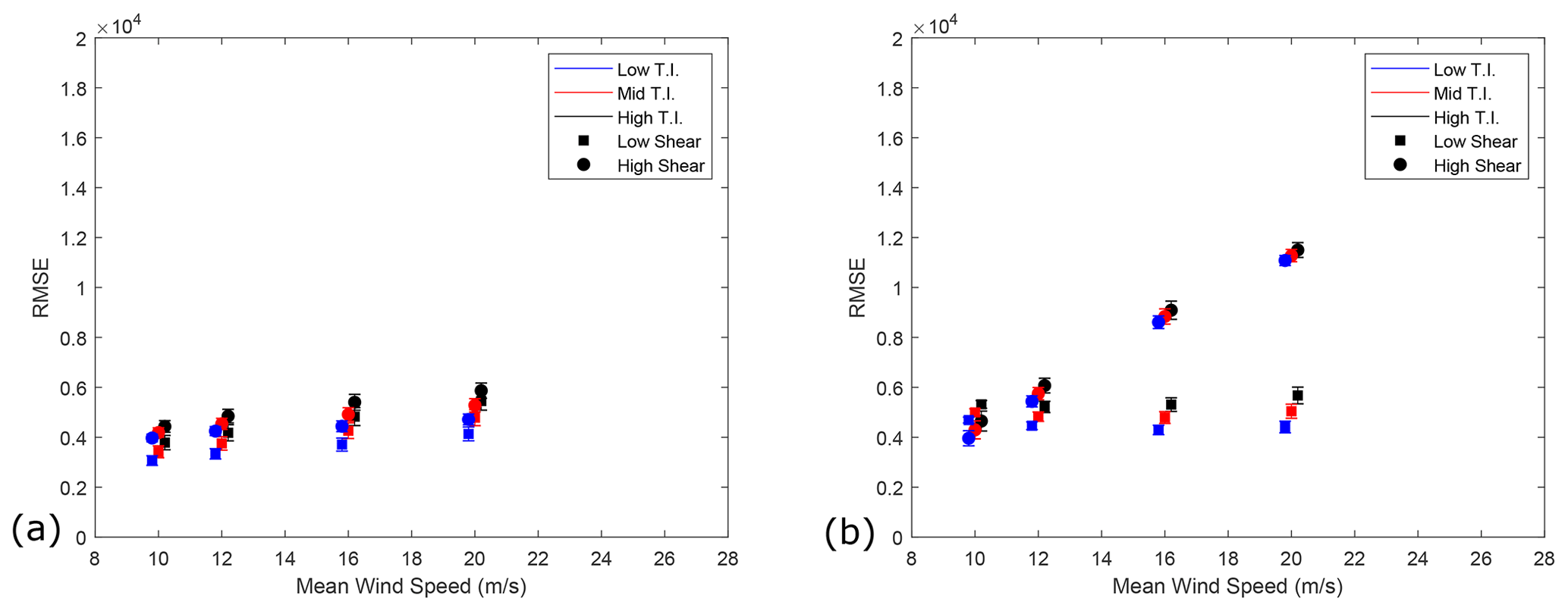
Figure 5(a) RMSE between reaction forces from the analytical and DSRB FE model in the horizontal plane. The mean and standard deviations within each CPLS are plotted, staggered about mean wind speed for clarity. (b) RMSE reaction force results between the analytical and DSRB FE model in the vertical plane. The mean and standard deviations within each CPLS are plotted, staggered about mean wind speed for clarity.
Figure 5 displays RMSE results between the analytical model and the DSRB FE model in the horizontal and vertical planes. The accuracy of the analytical model in the horizontal axis appears to have slight sensitivities to wind speed and shear exponents, decreasing as their values increase. The RMSE results for the bearing reaction force in the vertical axis are more differentiated by the varying wind parameters than in the horizontal axis. The low-shear results remain fairly constant with increasing wind speed, although increasing sensitivity to TI with increasing wind speed can be seen. The high-shear exponent results are more sensitive to wind speed, with RMSE values increasing with wind speed. To put these results into context, the mean percentage error between resultant force magnitudes for the two models across all wind files is 1.54 %, with a mean correlation coefficient of 0.9996. These results indicate that the analytical model does in fact give good results across all tested wind profiles in both planes when compared with 3D model outputs. This conclusion is reinforced when one considers time series of these loads, with examples shown in Fig. 6.
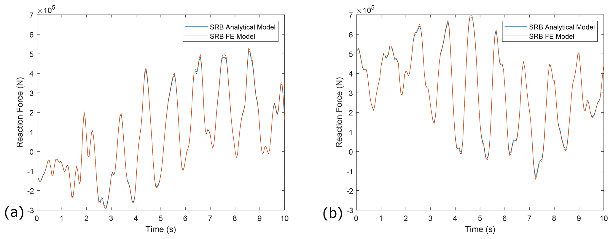
Figure 6(a) Example time series of reaction force results in the horizontal plane from the analytical and DSRB FE models. (b) Example time series of reaction force results in the vertical plane from analytical and DSRB FE models.
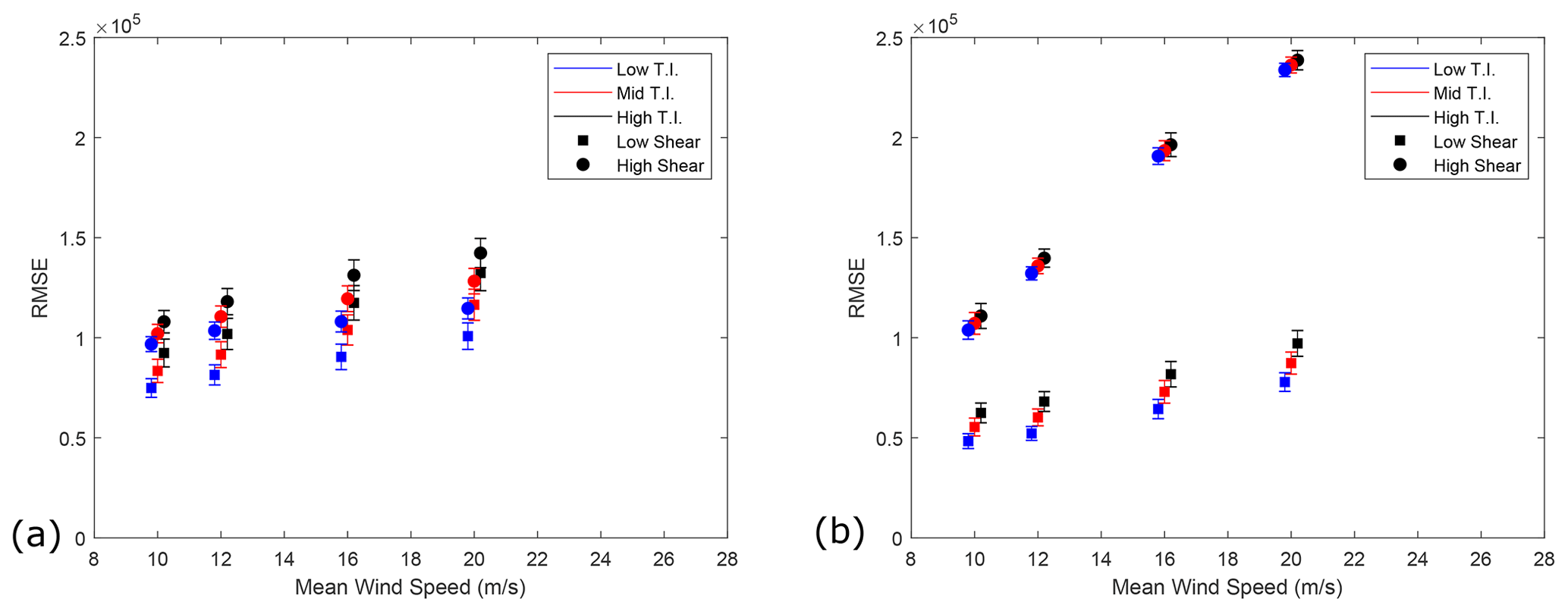
Figure 7(a) RMSE between reaction forces from the analytical and DTRB FE model in the horizontal plane. The mean and standard deviations within each CPLS are plotted, staggered about mean wind speed for clarity. (b) RMSE reaction force results between the analytical and DTRB FE model in the vertical plane. The mean and standard deviations within each CPLS are plotted, staggered about mean wind speed for clarity.
The analytical model reaction force results were then compared with the DTRB FE model, with the results displayed in Fig. 7. The analytical model shows a trend of decreasing accuracy with increasing wind speed and shear in the horizontal plane. Compared to the previous results, error values can be seen to have significantly increased by more than a factor of 10. The accuracy of the model in the vertical plane is highly sensitive to wind shear. Increasing mean wind speeds and TI slightly decrease the accuracy of the low-shear results in the vertical plane. In contrast, the high-shear exponent results in the vertical plane significantly decrease in accuracy with increasing mean wind speeds and show less sensitivity to TI. The mean percentage error and correlation coefficient were again considered between resultant force magnitudes across all wind cases. The mean error was found to be 22.74 %, and a mean correlation coefficient of 0.7781 was calculated, showing that the analytical model is noticeably less accurate in the DTRB moment-reacting case. This conclusion is again reinforced by time series of model outputs, examples of which are shown in Fig. 8.

Figure 8(a) Example time series of reaction force results in the horizontal plane from the analytical and DTRB FE models. (b) Example time series of reaction force results in the vertical plane from analytical and DTRB FE models.
The above comparisons suggest that the orthogonal independence and simple support assumptions made in the analytical model still allow for valid force outputs when representing a DSRB. However, the results also show that the analytical model has significantly overestimated the force reactions for the DTRB system. This motivates the derivation of a new analytical model to try and emulate the positive results seen in the DSRB case for moment-reacting DTRBs. Such a model is developed in the following section.
In order to allow moment reactions at the MB, torsional springs were added to the fixed bearing support in both planes of the analytical model. Thus, a new analytical model was created, displayed in Fig. 9a. The set of equations for the new analytical model are statically indeterminate, and so the model must be decoupled to find a solution (Hibbeler, 2011; Leet and Uang, 2011). The model was first simplified by moving the location of the force applied by the rotor mass, B, and associated overturning moment, M, to be positioned at the bearing support mount as shown in Fig. 9b. The model was then decoupled into two deflection models: one which has the rotor weight and overturning moment acting on the structure (Fig. 10a) and one which has the reaction moment from the torsional spring acting on the structure (Fig. 10b).

Figure 9(a) Analytical model for single-main-bearing set-up with torsional spring to include moment reactions. The overall model consists of one in the horizontal and one in the vertical plane. (b) Simplified analytical model with torsional spring.
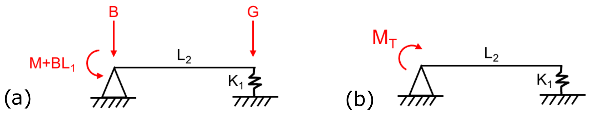
Figure 10(a) Deflection model 1 (rotor weight and overturning moment). (b) Deflection model 2 (torsional-spring reaction force).
The two deflection models can then be decoupled again to show the two mechanisms causing deflection in the shaft: bending of the beam due to the applied moment and rotation about the MB support due to spring support (gearbox) compression or extension. As the deflection mechanisms and equation derivation process are similar for the overturning moment and spring reaction moment on the system, only the equations and deflection mechanisms for the overturning moment are presented here. The two deflection mechanisms for the decoupled model with overturning moment and rotor weight are shown in Fig. 11.

Calculating θ11 as seen in Fig. 11 can be done by utilising the beam deflection formula shown in Eq. (2) (Popov, 1990).
The compression or extension length, y, of the spring must first be found before calculating θ12. For a loaded spring with stiffness K1, the distance stretched or compressed, y, is equal to the reaction force divided by the stiffness.
Trigonometrically, the deflection angle is then
and a small-angle approximation simplifies the equation to
and combining with Eq. (3) for y gives
The second set of deflection equations with respect to the reaction moment of the torsional spring on the shaft are calculated using the same method, with the angles of rotation labelled θ21 and θ22 and taking values of
and
The rotation of the torsional spring, θTS, is given by
where KR is the stiffness of the torsional spring and MT the reaction moment. The rotation of the torsional spring is also equal to the sum of all deflection angles, with positive and negative signs indicating direction:
The reaction forces RB and RT are still unknowns, and the above equation cannot be solved until the forces are balanced on the decoupled models. Balancing the moments about the bearing support in Fig. 12a gives
from which it follows
Similarly, moments can be balanced about the bearing support for the decoupled model loaded with the reaction moment from the torsional spring displayed in Fig. 12b, giving
and hence
These expressions for RB and RT can now be entered into Eqs. (6) and (8), respectively, resulting in solvable equations for θ12 and θ22:
Equation (10) can therefore be written in full in terms of known quantities as
and rearranged for MT as
The equation for the reaction moment from the torsional spring, MT, has been derived, and, as such, the system is now statically determinate. A moment balance can be performed on the gearbox support over the whole system, as shown in Fig. 13, to derive the reaction force at the bearing support, RA:
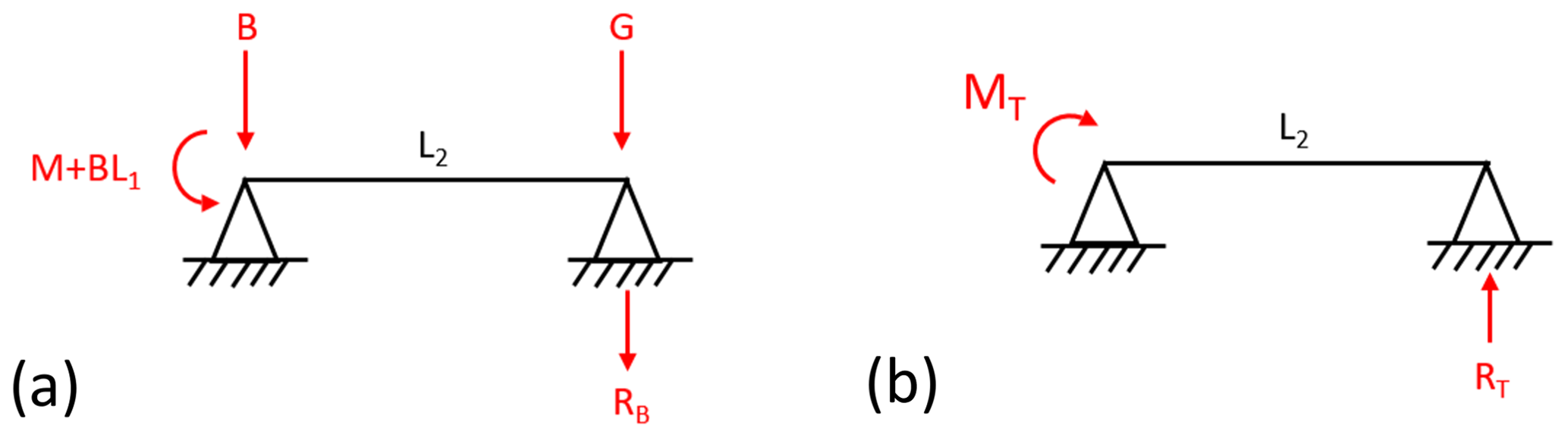
Figure 12(a) Force balance corresponding to deflection model 1. (b) Force balance corresponding to deflection model 2.
5.1 Estimating torsional-spring stiffness
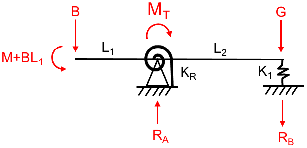
Having derived the relevant equations for a new analytical model with moment reaction capabilities, it is then necessary to determine appropriate spring-stiffness values in each plane. These were estimated using the FE DTRB model. The body-to-ground springs representing the shaft connection to the gearbox were removed from the model and four nodes selected: one at the bedplate connection and one at the top of the bearing housing for the vertical plane and one on both sides of the bearing housing at points of mid-height and mid-thickness for the horizontal plane. Known moments were then applied about the horizontal and vertical axes separately and the displacement of the nodes recorded. The angle of rotation about the midpoint of the vertical nodes was calculated and used to determine the vertical-axis spring stiffness via the standard spring equation (Eq. 20). Likewise, the angle of rotation about the centre of the housing between the pre- and post-loaded nodal points was calculated and the torsional-spring stiffness about the horizontal axis estimated. These steps are illustrated in Figs. 14 and 15.
The two estimated spring-stiffness values, approximately 392 kNm rad−1 in the horizontal plane and 145 kNm rad−1 in the vertical plane, were then applied in the analytical DTRB model and the reaction forces at the bearing calculated across the wind profiles. Examining the time series plots of the reaction forces of the FE DTRB and the analytical DTRB models (Fig. 17), the new analytical model appears to capture the loading seen by the FE DTRB model very closely in both planes.
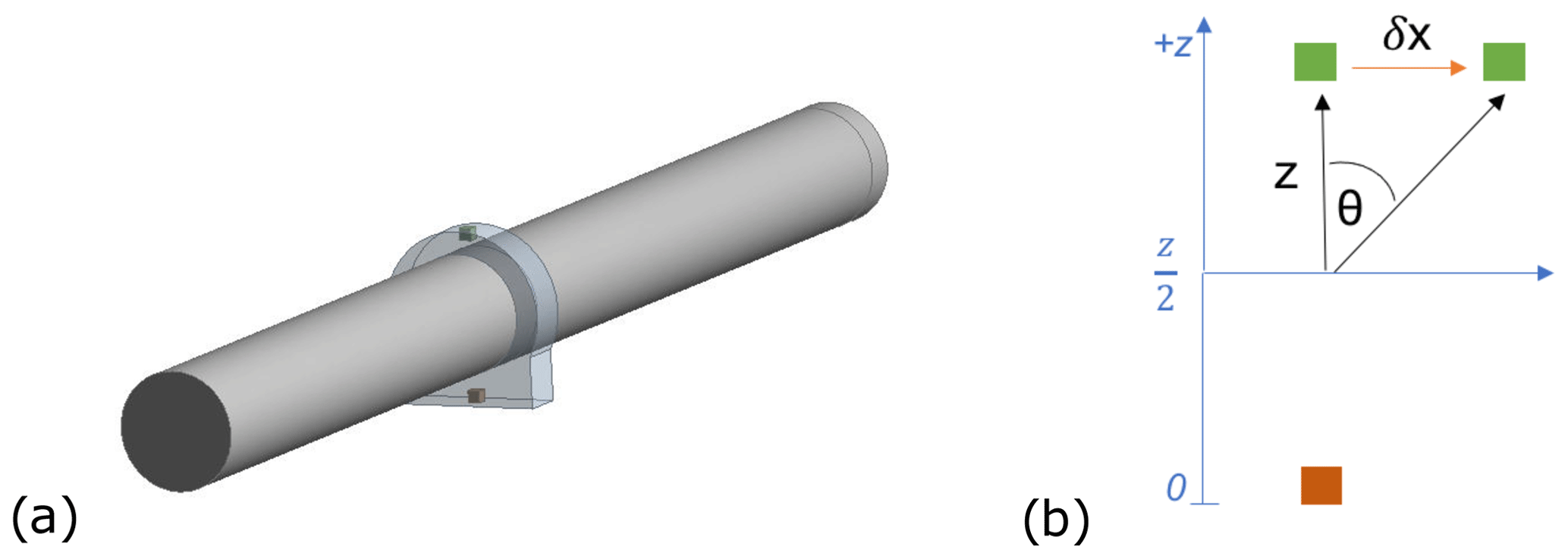
Figure 14Node selection within the bearing housing for estimating torsional-spring stiffness in the vertical plane.
Figure 15Node selection within the bearing housing for estimating torsional-spring stiffness in the horizontal plane.
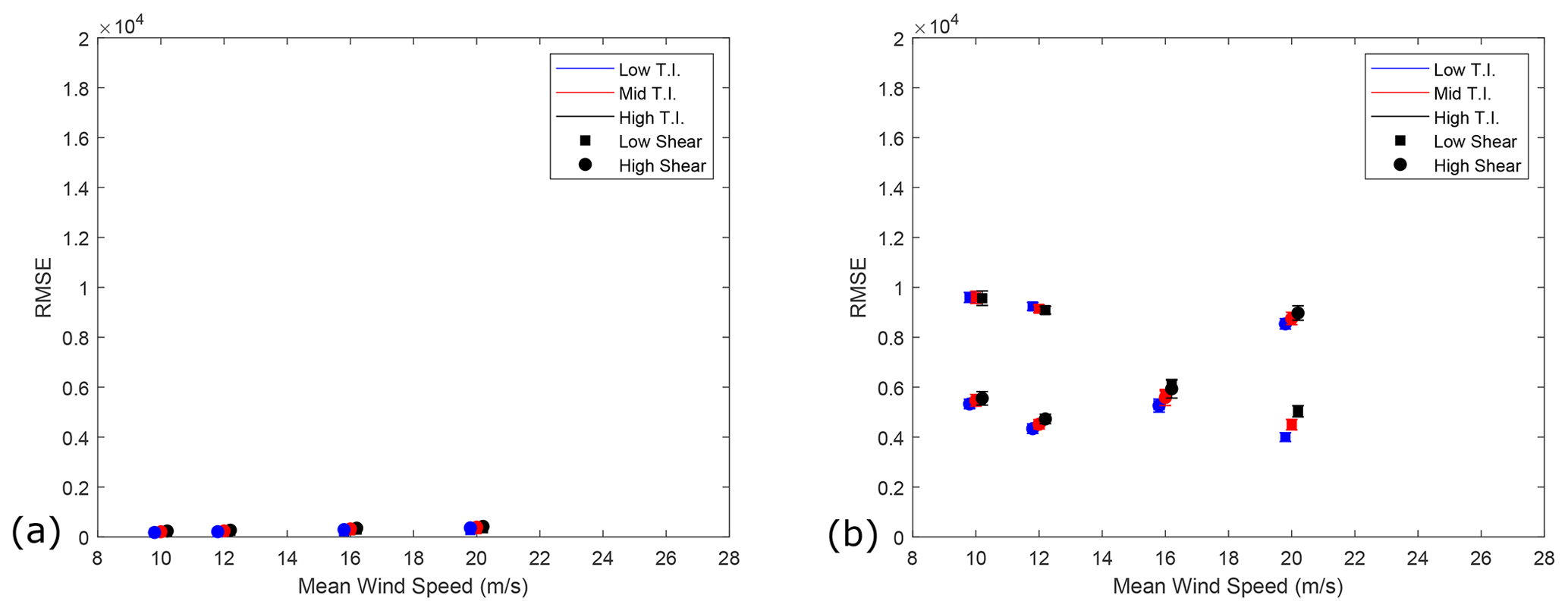
Figure 16(a) RMSE between reaction forces from the analytical DTRB (with torsional springs) and DTRB FE model in the horizontal plane. The mean and standard deviations within each CPLS are plotted, staggered about mean wind speed for clarity. (b) RMSE reaction force results between the analytical DTRB (with torsional springs) and DTRB FE model in the vertical plane. The mean and standard deviations within each CPLS are plotted, staggered about mean wind speed for clarity.
RMSE results in this case are plotted in Fig. 16. It can be seen from the plots that the inclusion of the torsional springs greatly reduces the RMSE values as well as variance within each CPLS between the analytical and DTRB FE models in both the horizontal and vertical planes. The mean absolute error and mean correlation coefficients between resultant force magnitudes were calculated for the two models; mean percentage error in this case has dropped to 1.61 %, while the mean correlation coefficient has increased to 0.9996. The results in Fig. 16 show shear profile to have the strongest effect on model accuracy in the vertical plane. It can also be seen that the low-shear cases accuracy increases with increasing mean wind speed, while the high-shear cases accuracy decreases with increasing mean wind speed.
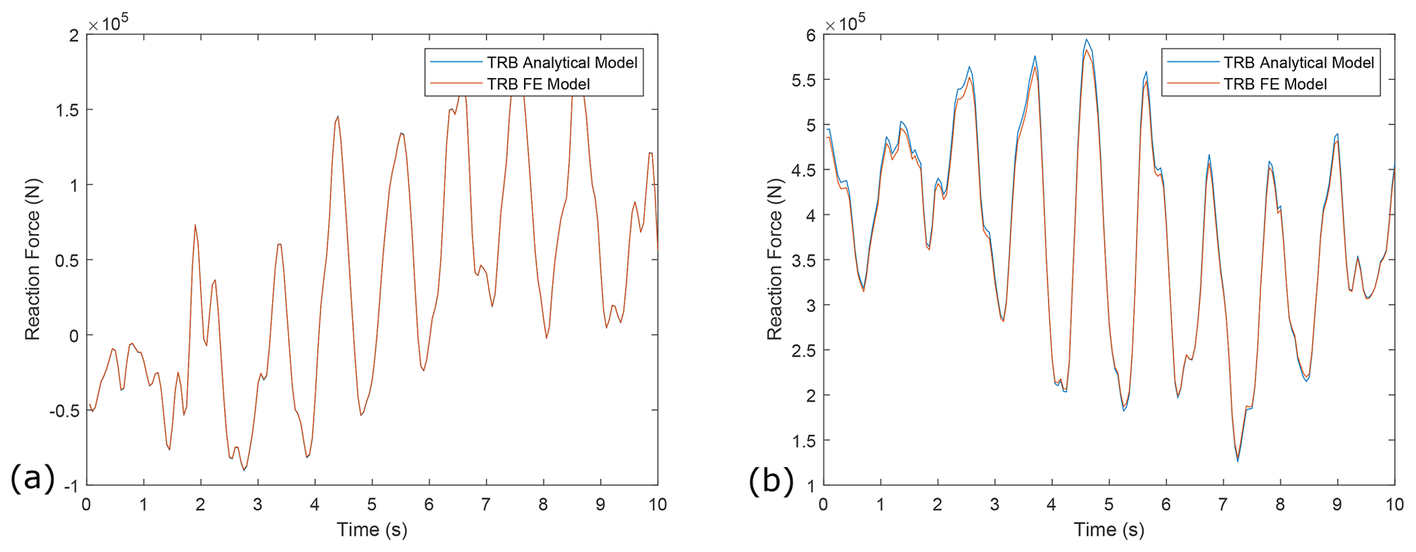
Figure 17(a) Example time series of reaction force results in the horizontal plane from the analytical DTRB (with torsional springs) and DTRB FE models. (b) Example time series of reaction force results in the vertical plane from analytical DTRB (with torsional springs) and DTRB FE models.
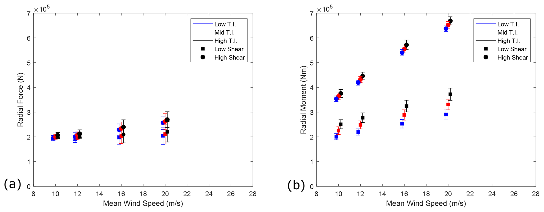
Figure 18(a) Mean radial resultant force magnitudes from the analytical DTRB model. Mean and standard deviations within each CPLS are plotted, staggered about mean wind speeds for clarity. (b) Mean resultant moment magnitudes from the analytical DTRB model. Mean and standard deviations within each CPLS are plotted, staggered about mean wind speeds for clarity.
Presented results imply that the analytical SMB model used in Hart et al. (2019) and the analytical moment-reacting model developed here provide good representations of DSRB- and DTRB-type reaction forces (and moments in the latter case), respectively. Whereas in previous work the mean and peak loads across operating points were considered, here these same values are investigated for the DTRB case using the analytical DTRB model, with the original being referred to as the analytical DSRB model.
The mean radial loading for the analytical DSRB model in the previous study showed high sensitivity to shear exponent, with the low-shear exponent wind files resulting in larger radial loading. Plotted low-shear results lay between 400 and 500 kN; similarly, high-shear exponent plotted results were between around 200 and 300 kN. The mean loads within each CPLS remained fairly constant, with small standard deviations, and TI had some effect on the results, with higher TI resulting in slightly higher loading.

Figure 19(a) Peak radial resultant force magnitudes from the analytical DTRB model. Mean and standard deviations within each CPLS are plotted, staggered about mean wind speeds for clarity. (b) Peak resultant moment magnitudes from the analytical DTRB model. Mean and standard deviations within each CPLS are plotted, staggered about mean wind speeds for clarity.
Mean radial force and moment results for the analytical DTRB model are shown in Fig. 18. The presence of moment as well as force reactions can be seen to have reduced the mean radial force loading across the full envelope of wind conditions when compared with results in Hart et al. (2019) while also reducing the system's sensitivity to shear profile. The mean force loads within each CPLS remain fairly constant, with small deviations at low mean wind speeds, although deviations increase with increasing wind speeds.
Considering moment reactions, the magnitude increases with increasing mean wind speeds, and the high-shear cases contribute to larger moment loading compared to low-shear cases. There are also sensitivities to TI in both shear exponent cases.
The analytical DSRB peak radial loads presented in Hart et al. (2019) show peak loads increasing in size and variability with increasing wind speeds. The peak loads see significant changes with TI but are most sensitive to shear exponent. Plotted results fall within 500 and 1200 kN. The plotted mean peak radial reaction forces in the SMB system with a DTRB fall within the range of approximately 510 to 955 kN and show a reduced sensitivity to shear exponent as shown in Fig. 19. The overall trend of the results displays magnitude and variability increasing with mean wind speed. The peak moment loads show high overall sensitivity to shear exponent, TI, and mean wind speed. The variability in peak moment loads also increases with wind speed.
The previous sections have outlined how the original SMB analytical model can be extended to recreate moment-reacting behaviour at the MB. It is worth considering the practicalities of this approach given that determining torsional-spring-stiffness values requires access to an FE model. Two pertinent questions related to this are therefore as follows: (1) if one requires an FE model in the first place, why cannot all analysis be undertaken using it instead of the simplified representations proposed here? (2) Is it practical to assume that an FE model will be available in general? With respect to the first question, there are two main considerations which imply that simplified models will likely be necessary. First, as has been touched upon, analysis over large numbers of load cases and/or turbines becomes infeasible for high-complexity models due to processing power requirements. In addition, any MB load model which might be embedded within existing aeroelastic software would likewise need to be computationally efficient (see e.g. Girsang et al., 2014). Considering the second question, detailed FE models of the drivetrain will commonly be used as part of the wind turbine design process. However, such models may well not be owned by or accessible to the wind farm operator. Despite this, the required spring-stiffness values for simplified representations could be requested from the designer or manufacturer given that required parameters are unlikely to be considered sensitive or proprietary. In addition, it may transpire that sensible spring stiffnesses can be identified which allow operators to select appropriate values based on drivetrain dimensions and geometry without requiring access to detailed models; this possibility will be explored in future work.
To be clear, the detailed and high-quality models used in existing work and outlined in Sect. 2 will remain crucial to the study of MB loading and operational behaviour. Rather than seeking to compete with such models, it is instead suggested that there are important synergies. For example, broader studies using simplified models can be leveraged to identify specific load cases requiring more detailed investigation with higher-complexity models. Similarly, the MB load outputs of simple representations, obtained from coupling with aeroelastic code, can be used as inputs to more detailed models of bearing internal and external structure, allowing detailed studies to take place while preserving a level of modularity.
This paper considers the question of whether analytical models can be used to effectively evaluate load reactions for 3D main-bearing support configurations with either moment-reacting or non-moment-reacting behaviours. The results of comparisons with 3D FE drivetrain models, designed to exhibit the relevant load reaction properties, indicate that the existing single-main-bearing analytical model can well represent bearing reaction forces in the non-moment-reacting case (e.g. double-row spherical roller bearings). However, it was also shown to be unsuitable for cases where a support has moment-reacting capabilities (e.g. double-row tapered roller bearings). Therefore, a second analytical model was created through the addition of torsional springs to represent a bearing which supports moments as well as forces. Spring stiffnesses were found for this model using a static analysis of the FE model. Outputs from the new analytical model were compared with the moment-reacting 3D model, with results indicating that it offers a greatly improved tool for analysis in the moment-reacting case. The developed model was then used to consider mean and peak forces and moment reactions for this type of bearing across a range of operating conditions.
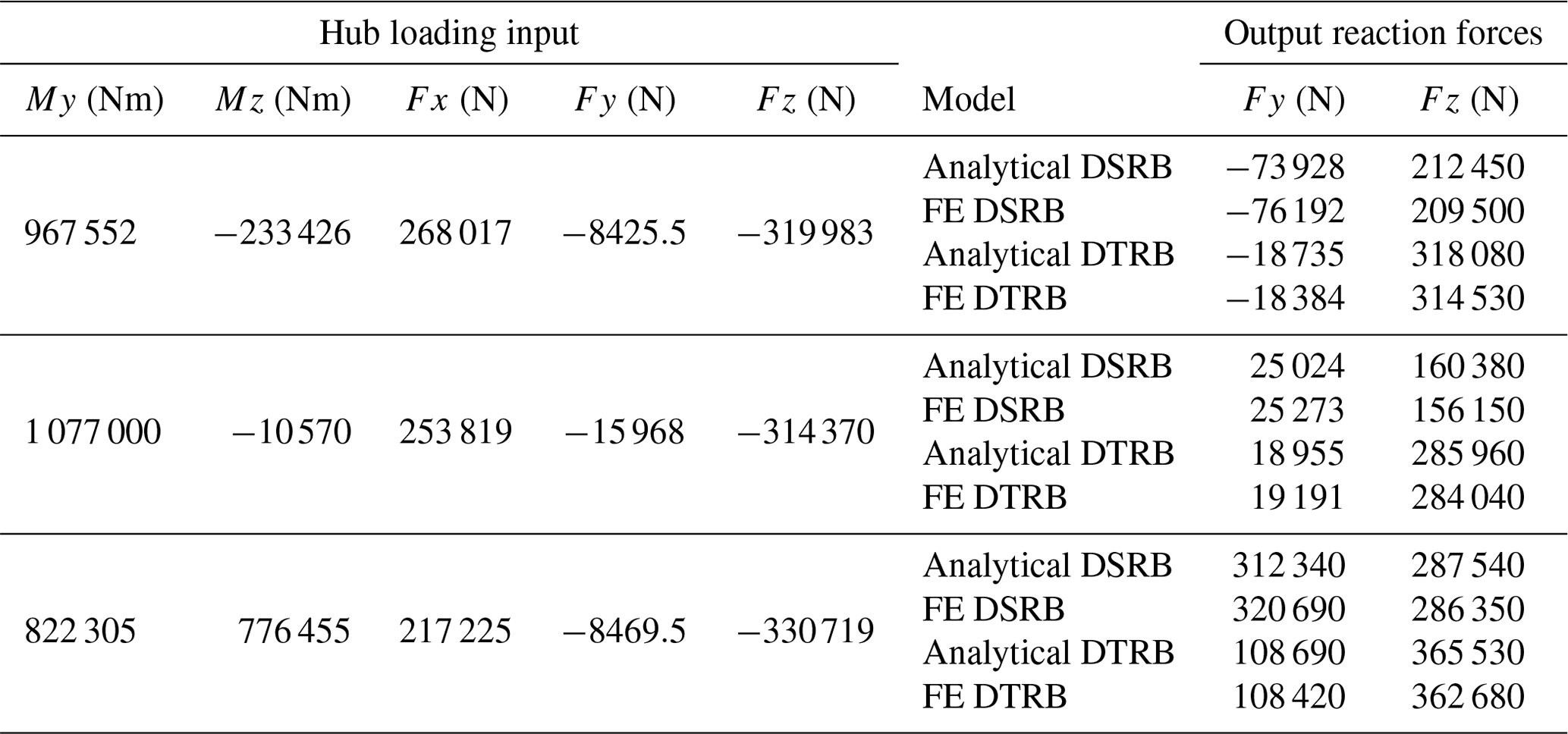
Table A1 contains example input and output values for all models used in this work.
Table A1Hub loading inputs and corresponding model outputs at various time steps. Quantities are in the DNV GL Bladed reference frame.
A shaft sensitivity analysis was carried out to explore the effect of shaft thickness and therefore stiffness on the MB reaction force results for each model. The implemented models are assumed to have solid shafts; however, main shafts typically have small boreholes throughout the centre to allow for the passing of electrical cables. Therefore, thicknesses of 100 %, 75 %, and 50 % were compared to conservatively cover typical main shaft thicknesses and ensure the solid-shaft assumption does not impact the results of this work. Results are plotted below for the analytical DTRB, FE DSRB, and FE DTRB models, respectively. These results, in which only very small deviations can be seen, indicate that shaft thickness appears to have a minimal effect on model accuracy.
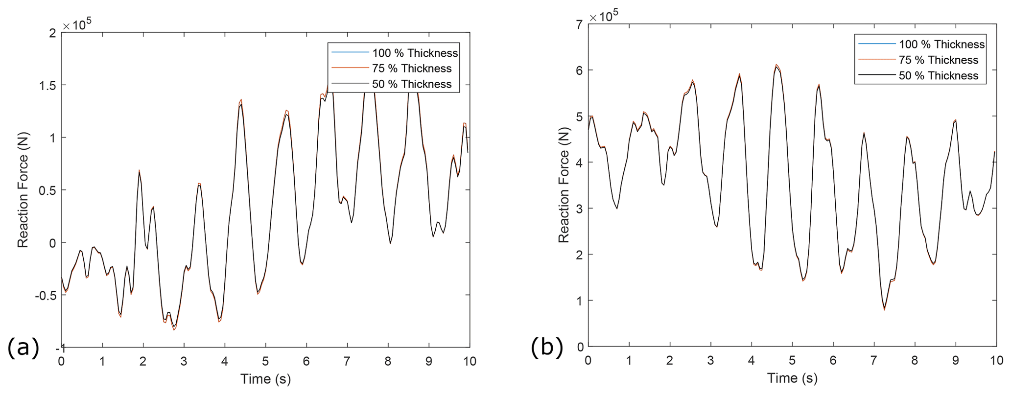
Figure B1(a) Example time series of reaction force results in the horizontal plane from the analytical DTRB (with torsional springs) model when the shaft thickness is altered. (b) Example time series of reaction force results in the vertical plane from the analytical DTRB (with torsional springs) model when the shaft thickness is altered.
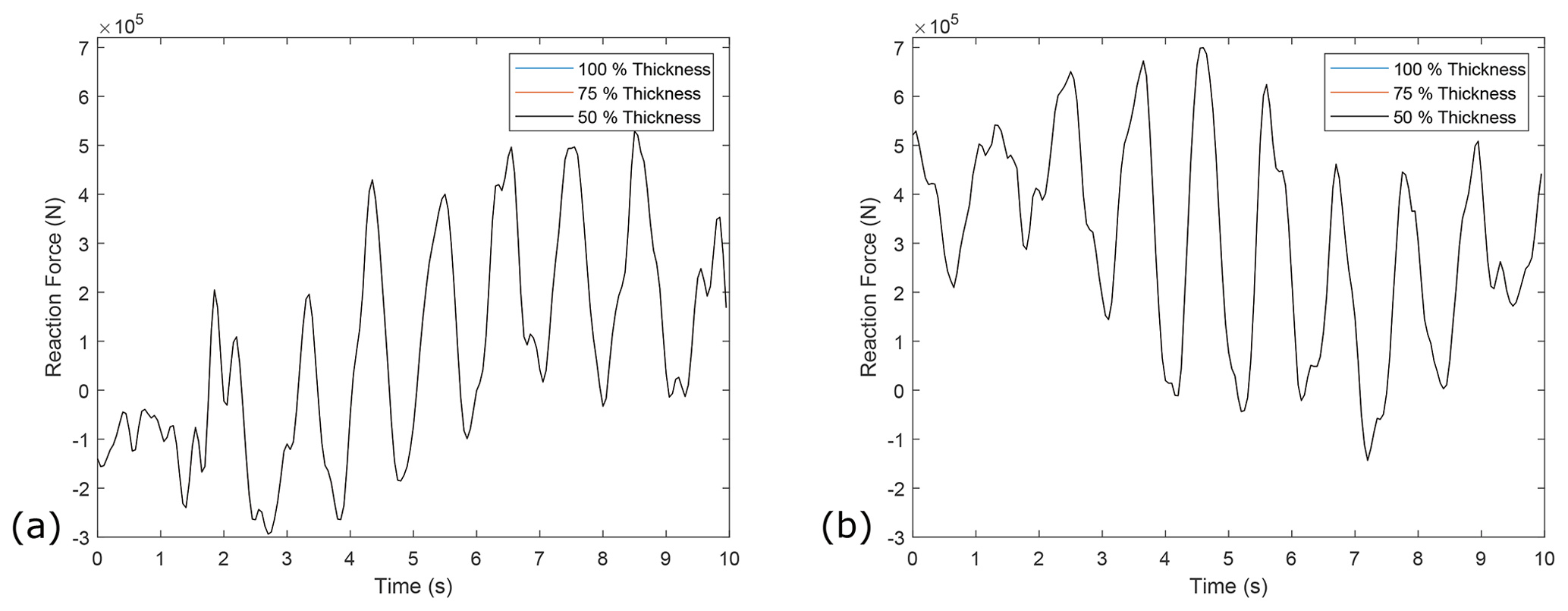
Figure B2(a) Example time series of reaction force results in the horizontal plane from the FE DSRB model when the shaft thickness is altered. (b) Example time series of reaction force results in the vertical plane from the FE DSRB model when the shaft thickness is altered.
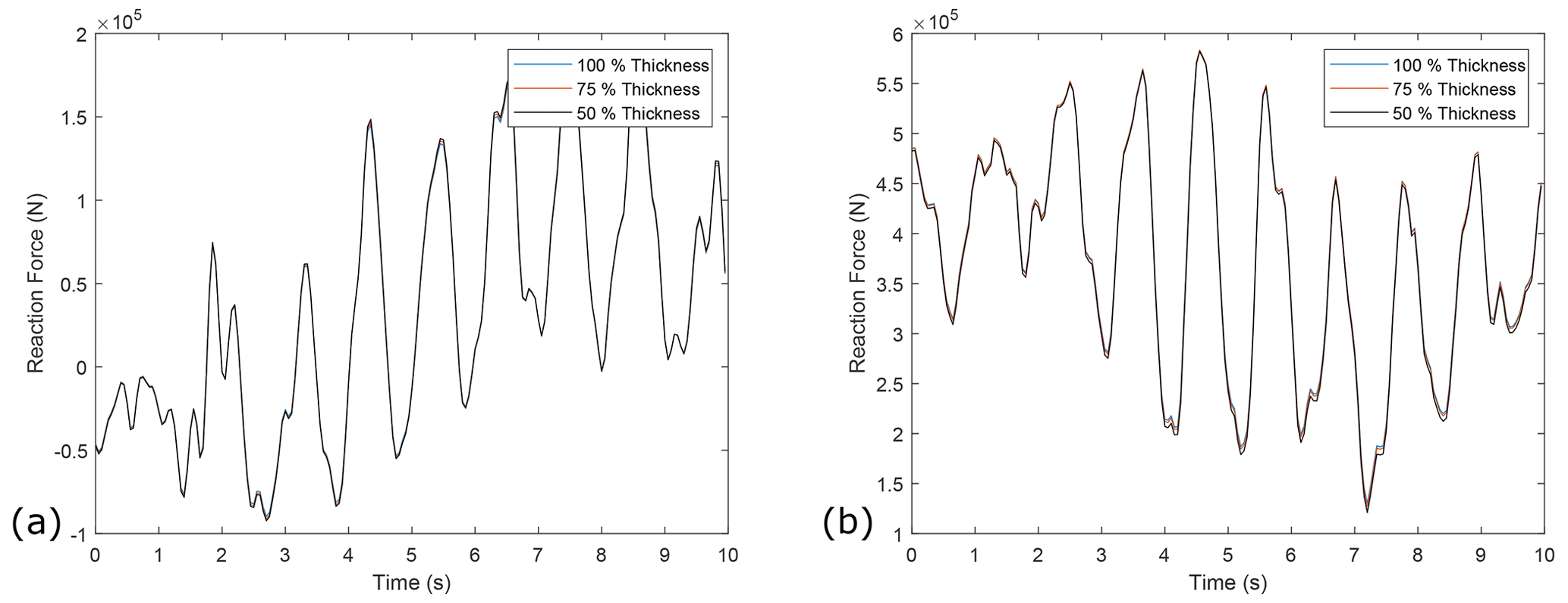
Figure B3(a) Example time series of reaction force results in the horizontal plane from the FE DTRB model when the shaft thickness is altered. (b) Example time series of reaction force results in the vertical plane from the FE DTRB model when the shaft thickness is altered.
Computer code and data used throughout this paper will be made available on request. Please contact the lead author for more information.
JS was the main researcher and also led the writing of the manuscript. EH and AKA supported model development, results analysis, and manuscript preparation.
The authors declare that they have no conflict of interest.
This article is part of the special issue “WindEurope Offshore 2019”. It is a result of the WindEurope Offshore 2019, Copenhagen, Denmark, 26–28 November 2019.
The authors would like to acknowledge extensive support throughout this work from Onyx Insight, specifically Robin Elliott, Rhys Evans, and Evgenia Golysheva.
This research has been supported by the Engineering and Physical Sciences Research Council (grant no. EP/L016680/1).
This paper was edited by Charlotte Bay Hasager and reviewed by Fabian Schwack, Ron A. J. van Ostayen, and one anonymous referee.
Artigao, E., Martín-Martínez, S., Honrubia-Escribano, A., and Gómez-Lázaro, E.: Wind turbine reliability: A comprehensive review towards effective condition monitoring development, Appl. Energy, 228, 1569–1583, https://doi.org/10.1016/j.apenergy.2018.07.037, 2018. a
Bosmans, J., Blockmans, B., Croes, J., Vermaut, M., and Desmet, W.: 1D–3D Nesting: Embedding reduced order flexible multibody models in system-level wind turbine drivetrain models, in: Conference for Wind Power Drives, 12–13 March 2019, Aachen, 523–537, 2019. a
Cardaun, M., Roscher, B., Schelenz, R., and Jacobs, G.: Analysis of wind-turbine main bearing loads due to constant yaw misalignments over a 20 years timespan, Energies, 12, 1768, https://doi.org/10.3390/en12091768, 2019. a
Dowson, D. and Higginson, G. R.: Elastohydrodynamic Lubrication – Chapter 12, in: vol. 23, Pergamon Press Ltd., Oxford, England, 1977. a
Girsang, I. P., Dhupia, J. S., Muljadi, E., Singh, M., and Pao, L. Y.: Gearbox and drivetrain models to study dynamic effects of modern wind turbines, IEEE T. Indust. Appl., 50, 3777–3786, https://doi.org/10.1109/TIA.2014.2321029, 2014. a
Harris, T. A.: Essential Concepts of Bearing Technology, 5th Edn., CRC Press, Boca Raton, Florida, https://doi.org/10.1201/9781420006599, 2006. a
Hart, E.: Developing a systematic approach to the analysis of time-varying main-bearing loads for wind turbines, Wind Energy, 23, 2150–2165, https://doi.org/10.1002/we.2549, 2020. a, b
Hart, E., Turnbull, A., Feuchtwang, J., McMillan, D., Golysheva, E., and Elliott, R.: Wind turbine main‐bearing loading and wind field characteristics, Wind Energy, 22, 1534–1547, https://doi.org/10.1002/we.2386, 2019. a, b, c, d, e, f, g, h, i, j, k
Hart, E., Clarke, B., Nicholas, G., Kazemi Amiri, A., Stirling, J., Carroll, J., Dwyer-Joyce, R., McDonald, A., and Long, H.: A review of wind turbine main bearings: design, operation, modelling, damage mechanisms and fault detection, Wind Energ. Sci., 5, 105–124, https://doi.org/10.5194/wes-5-105-2020, 2020. a, b
Hibbeler, R.: Structural Analysis, Pearson Education, University of Louisiana, Lafayette, 2011. a
IEC: Wind turbines – Part 1: Design requirements, Tech. rep., IEC, Geneva, Switzerland, 2005. a, b
Junginger, M., Faaij, A., and Turkenburg, W. C.: Cost Reduction Prospects for Offshore Wind Farms, Wind Eng., 28, 97–118, 2004. a
Keller, J., Shend, S., Cotrell, J., and Greco, A.: Wind turbine drivetrain reliability collaborative workshop: a recap, Tech. rep., US Department of Energy, available at: https://www.researchgate.net/publication/307511892 (last access: 23 December 2020), 2016. a
Kock, S., Jacobs, G., and Bosse, D.: Determination of Wind Turbine Main Bearing Load Distribution, J. Phys.: Conf. Ser., 1222, 012030, https://doi.org/10.1088/1742-6596/1222/1/012030, 2019. a, b
Leet, K. C. and Uang, A. G.: Fundamentals of Structural Analysis, McGraw Hill, Boston, 2011. a
Popov, E. P.: Engineering Mechanics of solids, Prentice-Hall Inc., Upper Saddle River, NJ, 1990. a
Sethuraman, L., Guo, Y., and Sheng, S.: Main Bearing Dynamics in Three-Point Suspension Drivetrains for Wind Turbines, in: American wind energy association windpower, 18–21 May 2015, Orlando, Florida, 2015. a
Sinha, Y. and Steel, J. A.: A progressive study into offshore wind farm maintenance optimisation using risk based failure analysis, Renew. Sustain. Energ. Rev., 42, 735–742, https://doi.org/10.1016/j.rser.2014.10.087, 2015. a
Smalley, J.: Turbine components: bearings, available at: http://www.windpowerengineering.com/design/mechanical (last access: 5 April 2019), 2015. a
Tavner, P. J., Xiang, J., and Spinato, F.: Reliability analysis for wind turbines, Wind Energy, 10, 1–18, https://doi.org/10.1002/we.204, 2007. a
Tibbits, P. A.: Fem simulation and life optimization of tandem roller thrust bearing, in: Proceedings of the ASME International Design Engineering Technical Conferences and Computers and Information in Engineering Conference – DETC2005, 3 A, 24–28 September 2005, Long Beach, California, USA, 79–88, https://doi.org/10.1115/detc2005-84234, 2005. a
UK Government: Contracts for Difference Second Allocation Round Results, Tech. Rep. September, UK Government, 2017. a
Wang, S., Nejad, A. R., Bachynski, E. ., and Moan, T.: Effects of bedplate flexibility on drivetrain dynamics: Case study of a 10 MW spar type floating wind turbine, Renew. Energy, 161, 808–824, https://doi.org/10.1016/j.renene.2020.07.148, 2020a. a, b
Wang, S., Nejad, A. R., and Moan, T.: On design, modelling, and analysis of a 10-MW medium-speed drivetrain for offshore wind turbines, Wind Energy, 23, 1099–1117, https://doi.org/10.1002/we.2476, 2020b. a
Wilkinson, M.: Measuring Wind Turbine Reliability – Results of the Reliawind Project, Tech. rep., GL Garrad Hassan, St Vincent's Works, Bristol, UK, https://doi.org/10.11333/jwea.35.2_102, 2011. a
Wind Europe: Wind Energy in Europe in 2019, Tech. rep., Wind Europe, available at: https://windeurope.org/wp-content/uploads/files/about-wind/statistics/WindEurope-Annual-Statistics-2019.pdf (last access: 26 February 2019), 2020. a
Yagi, S.: Bearings for Wind Turbine, 71, NTN Technical review, NTN, 40–47, 2004. a
- Abstract
- Introduction
- Background
- Finite-element models
- Comparison of analytical and finite-element models
- Extending the analytical model to include moment reactions
- Investigating mean and peak loads of an SMB with DSRB and DTRB supports
- Discussion
- Conclusions
- Appendix A: Input–output table
- Appendix B: Shaft sensitivity analysis
- Code and data availability
- Author contributions
- Competing interests
- Special issue statement
- Acknowledgements
- Financial support
- Review statement
- References